


Abstract
We propose a simple way of probing the number of modes contributing to the channeling in graphene waveguides which are formed by a gauge potential produced by mechanical strain. The energy mode structure for both homogeneous and non-homogeneous strain regimes is carefully studied using the continuum description of the Dirac equation. We found that high strain values privilege negative (instead of positive) group velocities throughout the guidance, sorting the types of modes flowing through it. We also show how the effect of a substrate-induced gap competes against the strain.
Export citation and abstract BibTeX RIS

Content from this work may be used under the terms of the Creative Commons Attribution-NonCommercial-ShareAlike 3.0 licence. Any further distribution of this work must maintain attribution to the author(s) and the title of the work, journal citation and DOI.
1. Introduction
In the last few decades, new carbon-based structures have been realized in the laboratory. Of them, graphene, a single-atom-thin sheet of hexagonal arranged carbon atoms, has drawn considerable attention due to its remarkable properties and a wide variety of potential applications in nanoelectronic devices [1, 2]. One exciting issue concerning graphene is that carrier densities can be varied over a large range by external electrostatic gates [3] and, as a consequence, p–n junctions based on this material can be built [4, 5]. It is possible to produce graphene-based electronic waveguides using p–n–p junctions in which the charge carriers act similarly as in optics and where the Fermi energy plays the role of the refraction index [6]. As a consequence, the guidance in this quasi-one-dimensional channel can be realized simply by controlling the Fermi energy in the two-dimensional (2D) graphene sheet.
Furthermore, the massless character of Dirac fermions in graphene allows the observation of the so-called Klein tunneling, which is the perfect transmission of charge carriers through electrostatic barriers for normal incidence [7–9]. Such a phenomenon leads to a poorer efficiency in the guidance of charge carriers along the interfaces of graphene p–n–p junctions [6] and might hamper the performance of graphene-based electronic channeling devices. The inherent difficulty of controlling such a phenomenon in p–n junctions remains an issue,but recent advances in strain engineering have opened up the possibility of handling the Klein tunneling problem.
In-plane strain effects can be understood as a perturbation in the nearest-neighbor hopping amplitude which induces an effective gauge potential in the Hamiltonian [10]. In fact, electronic properties in strained graphene are currently being studied both theoretically and experimentally [11–13]. The local strains in graphene can be tailored to produce new effects to manipulate electron transport in graphene waveguides [14, 15]. This is an important step toward all graphene electronics. Theoretical studies on the channeling in such devices are necessary and, as far as we know, they have not been reported until now.
In this work, we theoretically propose a simple way of probing the modes contributing in graphene waveguides which are formed through strain engineering. We explore the energy band structure for both homogeneous and non-homogeneous strain regimes and study these effects on the modes that contribute to guidance. The non-homogeneous regime can be obtained by tailoring the local stains and thus producing different magnetic strengths, in such a way that the magnetic barriers forming the guide should have different heights. In this case, we find that the energy-mode degeneracy of the total group velocity is lifted and quasiparticles with negative group velocity become the most likely charge flowing in the waveguide. We also map out the energy range and angles for which the device should operate more efficiently as the strain increases. Finally, we explore the effects due to the graphene–substrate interaction versus the strain parameter.
This paper is organized as follows. Section 2 is devoted to our theoretical formulation where we define the quantities used to count the guiding modes. In section 3, we present our numerical results and discussions. Finally, we present our conclusions in section 4.
2. Theoretical formalism
Figure 1 shows schematically the potential profile of the system under study. An electronic waveguide (of width L) in the y-direction is formed between different strained regions in the x-direction. Mechanical strain in graphene can be described by a gauge vector potential and produces high pseudo-magnetic fields [16]. But furthermore, a waveguide can be formed by strain-induced magnetic barriers in different regions. The magnetic barrier height is accounted for by the magnetization intensity Γy. The expression for such an intensity is shown and discussed below. The sample can be further covered by a thin layer of a dielectric material, over which the top-gate contacts might be placed forming the yellow barriers of height U0. In practice, the strain-induced gauge potential produces magnetic barriers, which creates a potential offset shown by dotted lines in figure 1. This offset creates three different regions for carriers. In contrast to the electrostatic potential, this sort of strain should be responsible for creating an effective confinement region where the guidance should take place, avoiding the weak confinement (Klein tunneling) usually seen when one is dealing with electrostatic barriers alone. Note that these regions could form the sort of potential profile resembling a p–n–p junction. In fact, if an electrostatic gate is applied to this region, it will induce a potential U0 in graphene with the same locations as the magnetic barriers helping to further create the junction, but now with a real possibility of confinement, so that the guidance occurs through region II. Incident angles θ for carriers inside the guide should be considered and total internal reflection permitted, in principle, by virtue of the presence of the magnetic barriers alone. In this sense, quasibound states in region II should form quantized modes which eventually contribute to the guidance.
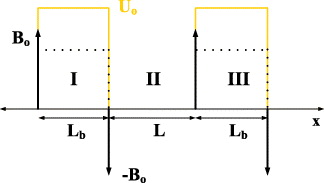
Figure 1. The resulting profile potential in the x-direction due to either a magnetic (dashed lines) or an electrostatic (yellow lines) barrier over the graphene sheet. In our calculations, we consider that Lb = 10 L.
Download figure:
Standard imageFor single-layer graphene in the presence of both a smooth electrostatic-gate potential and the mechanical strain, the low-energy quasiparticle Hamiltonian for a single valley can be described by the 2D Dirac equation [14]

where  is the wavevector, U(x) is the electrostatic potential as indicated in figure 1, which is assumed to be zero in region II and U0 = 100 meV in regions I and III,
  is the 2D Pauli vector and
  /2 is the lattice parameter with a0 = 0.246 nm and the hopping energy between the nearest neighbor t = 2.53 eV. Here β accounts for the coupling between graphene and the substrate that served as a host to the graphene. The substrate introduces different numbers of electrons in the sublattices A and B that form the unit cell of the graphene honeycomb. This is responsible for inducing a gap varying from 50 to 260 meV in substrates such as boron nitride [17]. The graphene is then tuned to the Dirac point when β = 0.
Note that the gauge potential 
 , which represents the mechanical strain, must be properly chosen to guarantee a constant (vector) potential in regions I and III. In fact, Ay should be a result of a combination of Heaviside functions which are reached when one considers the magnetic field as delta-functions provided by the two antiparallel magnetic fields [18–22] shown in figure 1. The magnetic barriers form a quantum well in the x-direction (region II) with a constant vector potential in regions I and III. The effective magnetic field in such a device is taken in the z-direction alone and is modeled by

where Lb (L) is the width of the magnetic barriers (well), with  the magnetic length, lB0 = 81.16 nm and field intensity B0 = 0.1 T. Here we consider that Lb = 10 L.
The translational invariance along the y-direction enforces solutions of equation (1) in the form Ψm(x,y) = eikyyϕm(x), with m = A and B being the sublattice indices (or the two pseudo-spinor components). Introducing this solution into the Hamiltonian H and after some algebra, we find a Helmholz-like equation

where Γy = B/B0 is a dimensionless parameter accounting for the strain intensity. Note that equation (2) is similar to the Helmholz equation [23] for electromagnetic waves. In obtaining this equation, one indeed demonstrates the real chances of treating optics-like phenomena in graphene electronic systems within the continuum description of the 2D Dirac equation.
The guidance might be obtained because the strain-induced interfaces produce three different regions for which three different types of solutions to equation (2) should be proposed. In analogy to the Goos–Hänchen effect [24, 25], we propose the component
which must decay exponentially in regions I and III and be stationary in region II. Here,

and

are taken as pure real numbers. By introducing the component ϕA(x) into the Hamiltonian in equation (1), the other pseudo-spinor component can be obtained straightforwardly and written as
where f± = γ(ky ± κ − Γyl−1B0)/(E − U0 + β) and λ ≡ ky. The usual boundary condition for the Goos–Hänchen effect is that both components ϕA(x) and ϕB(x), but not their derivatives, should be continuous functions at the interfaces x = ± L/2. Such a condition leads to a transcendental equation, whose roots provide the dispersion relation En(ky) for the guiding mode n [26, 27]. Note that  is the incident angle throughout the waveguide.
In order to study the guiding efficiency and probe (or sort) the modes contributing to it, we now consider the total flux Φ = ΦI + ΦII + ΦIII of quasiparticles flowing in the y-direction. Such a quantity is the total group velocity of charges flowing in the whole structure, i.e. in regions I–III all together. Here each flux Φi=I,II,III is calculated by integrating the corresponding current density  over the x-coordinate limiting each region [28]. The current densities (and so the group velocity) in regions I and III, where both pseudospinor components decay exponentially, are negative. In region II, where the pseudospin components are stationary wavefunctions, the current density (and also the group velocity) turns out to be positive. Because we are interested in the efficiency in the guidance region II, we define a dimensionless quantity

where ΦII is the flux in region II. We claim that the efficiency along the waveguide can be probed through equation (8), by sorting the type of modes contributing to the guidance. In the following, we show and discuss interesting and conclusive results based on such a definition.
3. Numerical results
In figure 2(a), we show how the dispersion relations En(θ) for the n = 6 lowest guiding modes change as the parameter Γy in the sample increases. Different colors show different intensities for the mechanical strain. We recall that  is the incident angle throughout the waveguide, so that the existence of different branches should indicate that the guidance might have been carried out with the same energy, but with different (quantized) values of the incident angle. As far as the strain is concerned, we consider here two different cases: (i) homogeneous and (ii) non-homogeneous mechanical strains. For such a purpose, we define an auxiliary parameter
  , which shows the difference between the strain intensity in regions I and III. Note that δ = 0 corresponds to the homogenous case as shown in figure 2(a) where the potential vector Ay is the same in regions I and III. Figure 2(a) shows the dispersion relation En(θ) for Γy = ΓIy = ΓIIIy running from 0 to 20. We see the dispersion relation En(θ) becoming more and more asymmetric with respect to θ when Γy increases, indicating clearly the breaking of mirror symmetry with respect to θ = 0° when only the K valley is considered. With increasing strain, each single branch En turns into a surface, shifting slightly to larger angles and allowing different values for the reflection mechanism. The most important effect here is perhaps the prevalence of negative angles over the positive ones as the mechanical strain reaches high values. Some branches even vanish for positive angles when the strain increases. We emphasize that this does not mean some particular excited (or fundamental) states that are missing because they are always present for negative values of θ. In fact, the prevalence for negative angles might be indicating a preferred way for K-valley holes (instead of electrons) to flow in the waveguide. By the same token, these results show that electrons (instead of holes) in the valley K' might be preferred to flow in the waveguide as the mechanical strain increases. This point has been addressed earlier [14] and will be further discussed below.

Figure 2. (a) Dispersion relation En(θ) surfaces for the six lowest guiding modes. The surface surges as the strain parameter Γy is continuously changed from 0 to 20. This range is shown in color scale. (b) The same as in part (a), but for the non-homogeneous case δ ≠ 0. Here, we keep ΓIy = 8 and vary ΓIIIy from 0 to 20 to obtain the color scale. The sample parameters are L = 50 nm, U0 = 100 meV, Lb = 10 L and β = 0 meV.
Download figure:
Standard imageIn figure 2(b), we show the same kind of perspective as in figure 2(a), but for δ ≠ 0. Here, we keep ΓIy = 8 and vary ΓIIIy from 0 to 20. We recall that such a non-homogeneous strain can be achieved by considering in figure 1 two different strengths, in such a way that the magnetic barriers in regions I and III are of different heights. We claim that this case should not be considered to be of pure academic interest only because the experimental setup seems to indicate that this might be some non-ideal situation that might eventually be reachable in the experiment. With this kind of picture one can clearly notice different guiding modes mixing up with each other as different surfaces join together. In fact, we see a strong coupling between different surfaces for some particular values for the parameter ΓIIIy. For instance, when the strain intensity ΓIIIy ≃ 8 there is a strong coupling between the fundamental and the first-excited modes for energies near U0. Their surfaces split into two parts, which can be seen for angles of about −60°, getting further coupled to the next excited mode. The dispersion relations as we saw here completely map out all the possible configurations for the dispersion relation En(θ) in the presence of the strain. It should serve as a motivation for further experimental studies concerning the coupling between different modes.
Based on the above discussion, one might be interested in knowing how strain can be used to probe (and sort), in a simple way, the number of modes contributing to the guidance efficiency. We will restrict ourselves here to the homogenous case alone, since our discussion will be similar whether the strain regime is changed or not. In the remaining study, we should be able to analyze the circumstances under which either the electron or the hole states are supposed to flow in the waveguide. As a consequence, we might be able to sort out which quasiparticle is mostly contributing to the efficiency of the waveguide.
In order to do that, we explore the definition in equation (8), which is the ratio of group velocities accounting for the effective (dimensionless) probability of having quasiparticles guided throughout region II. Note that η is a function of both the mode's energy En and the incident angle θ. In figure 3(a), we show all the projected planes when calculating and plotting η(En,θ) → y(z,x) for the case where δ = 0. Here, we keep Γy = ΓIy = ΓIIIy = 5 so that all other parameters are the same as in figure 2(a). Part (a) shows the dispersion relation En(θ) (the z–x plane) for the six lowest modes. We label the mode n by a superscript + (−) for positive (negative) angles. This result is a single curve of the surface seen in figure 2(a). The strain introduces an anisotropy with respect to the angles of incidence discussed before. Part (b) shows the corresponding z–y plane when plotting η(En,θ). Negative values for η account for those states that decay exponentially outside the waveguide, but still contribute to the guidance efficiency. These modes can also be seen as states that Klein-tunnel through the p–n interface, but equally contribute to the efficiency. In figure 3(c), we show the projection of the calculated η onto the x–y plane. Two points should be stressed here. (i) Note that the number of modes that reach η = −1 is larger than those reaching η = 1, since the mode n = 5− (but not the mode n = 5+) shows up due to increasing strain. Therefore, the modes with negative values of η should be the ones that contribute the most to the guidance. In this sense, the strain is also sorting the type of quasiparticle flowing throughout the waveguide. This is an effect that only strain imposes on the sample. (ii) The magnetic (vector) strain (potential) is responsible for breaking the energy degeneracy of the modes n− and n+ with respect to negative angles. Such a breaking is also seen in the z–y plane when the branches En=0− and En=0+ appear to be different from each other. In this sense, the negative (positive) values for θ represent holes (electrons) flowing in the waveguide.

Figure 3. Different projections of the calculated η(En,θ) → y(z,x) for Γy = 5 and δ = 0: (a) the z–x plane En(θ), (b) the z–y plane En(η) and (c) the efficiency η as a function of the incident angle θ. Different branches indicate the corresponding projection onto the z–x plane. The sample parameters are the same as in the previous figure.
Download figure:
Standard imageWe further explore these results and show in figure 4 that the strain effects might manifest themselves in experimental observations along the wire (waveguide). In order to do that, we define an auxiliary quantity

and plot it as a function of the energy E for Γy running from 0 to 5 with a step of 0.33. Note that, in figure 4, the thresholds of the plateaus occur at the positions as En(ky) reaches its minimum value. The quantity I(E) simply serves as a useful theoretical quantity for the transport experiments, since each minimum in the En(ky) should contribute with an amount of e2/h per spin and per valley to the conductance [24, 27]. Here, θn is the nth incident mode allowed for a given energy E. We claim that this quantity, as a function of energy, is a measure of the total mode contribution to the guidance. In fact, the lowest curve in figure 4(a), for Γy = 0, resembles the expected conductance along the wire in the absence of strain, because the mirror asymmetry in not present. Note that each additional plateau indicates a different mode contributing to guidance with increasing energy. The energy threshold for each plateau n is the lowest value of the corresponding energy En(ky) shown in the dispersion relation pictures in the lower panel of figure 4(b). As the strain Γy increases, the different modes which are studied above start contributing to the guidance and a richer structure appears by virtue of the breaking of the energy degeneracy of the modes n− and n+. To illustrate that, we show in the upper panel the same dispersion relation as in the lower one but now for Γy = 5. This is a reliable and simple way to view, probe and sort the modes contributing to the channeling in the waveguide which is treated within the continuum description of the 2D Dirac equation. We point out that the conductivity through the channel always takes place, even when β = 0, as shown by the lowest curve in figure 4. These effects are also studied in the literature by other authors [24].
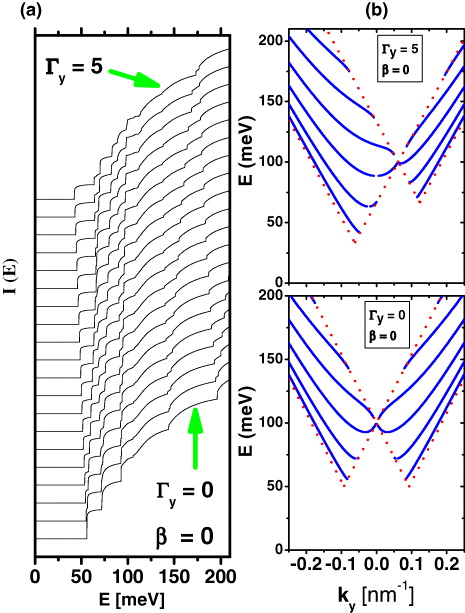
Figure 4. (a) The calculated I(E) resembling the conductance along the wire for Γy = 0. The same quantity is shown for Γy running up to 5 with a step of 0.33. Each plateau indicates the different modes getting into guidance as the energy increases. (b) Upper panel: the dispersion relation En(k) for Γy = β = 0; lower panel: En(k) for Γy = 5 and β = 0.
Download figure:
Standard imageFor the sake of completeness, we plot in figure 5 the same quantity as in figure 4, but now we keep Γy = 5 and vary the parameter β from 0 to 65 meV, with a step of 2.6 meV. For the highest curve, β = 65 meV, the energy threshold for each plateau n is exactly given by the lowest value of the corresponding energy En(ky) shown in figure 5(b). We see that the substrate-induced gap is responsible for recovering the mirror symmetry with respect to ky = 0 when a single valley K is considered. Such a symmetry is lost when strain is applied, but it is naturally recovered when both valleys K and K' are considered even in the absence of the induced gap.

Figure 5. The same quantity as in figure 4, but now we keep Γy = 5 and vary the parameter β from 0 to 65 meV. The inset shows the dispersion relation En(k) for Γy = 5 and β = 65 meV.
Download figure:
Standard image4. Conclusions
In summary, we theoretically propose a simple way of probing and sorting the modes contributing to the guidance efficiency in a strained-graphene-based waveguide treated within the continuum description of the Dirac equation. We also took into account an electrostatic gate potential in our formulation. We analyze the dispersion relation for both the homogeneous and the non-homogeneous strain and found different modes becoming mixed for certain incident angles. Our results show that Klein-tunneling (hole) states equally contribute to guidance when strain is applied, so that strain can sort and probe the kind of quasiparticle contributing to the efficiency. We have also shown that the substrate-induced gap in graphene might recover the mirror symmetry with respect of ky = 0 even if just a single valley is considered.
Acknowledgments
This work was supported by FAPESP, CNPq and the Flemish Science Foundation (FWO-Vl).