

Abstract
Approaches from metrology can assist earth observation (EO) practitioners to develop quantitative characterisation of uncertainty in EO data. This is necessary for the credibility of statements based on Earth observations in relation to topics of public concern, particularly climate and environmental change. This paper presents the application of metrological uncertainty analysis to historical Earth observations from satellites, and is intended to aid mutual understanding of metrology and EO. The nature of satellite observations is summarised for different EO data processing levels, and key metrological nomenclature and principles for uncertainty characterisation are reviewed. We then address metrological approaches to developing estimates of uncertainty that are traceable from the satellite sensor, through levels of data processing, to products describing the evolution of the geophysical state of the Earth. EO radiances have errors with complex error correlation structures that are significant when performing common higher-level transformations of EO imagery. Principles of measurement-function-centred uncertainty analysis are described that apply sequentially to each EO data processing level. Practical tools for organising and traceably documenting uncertainty analysis are presented. We illustrate these principles and tools with examples including some specific sources of error seen in EO satellite data as well as with an example of the estimation of sea surface temperature from satellite infra-red imagery. This includes a simulation-based estimate for the error distribution of clear-sky infra-red brightness temperature in which calibration uncertainty and digitisation are found to dominate. The propagation of these errors to sea surface temperature is then presented, illustrating the relevance of the approach to derivation of EO-based climate datasets. We conclude with a discussion arguing that there is broad scope and need for improvement in EO practice as a measurement science. EO practitioners and metrologists willing to extend and adapt their disciplinary knowledge to meet this need can make valuable contributions to EO.
Export citation and abstract BibTeX RIS

Original content from this work may be used under the terms of the Creative Commons Attribution 3.0 licence. Any further distribution of this work must maintain attribution to the author(s) and the title of the work, journal citation and DOI.
Glossary
| AVHRR | Advanced very high resolution radiometer |
| BT | Brightness temperature |
| CCI3 | Climate change initiative |
| CDR | Climate data record |
| CEOS | Committee on Earth observation satellites |
| ECMWF | European centre for medium-range weather forecasting |
| EO | Earth observation |
| ERA-Interim | Interim version of the ECMWF numerical weather prediction re-analysis |
| ESA | European space agency |
| FIDUCEO3 | Fidelity and uncertainty in climate data records from earth observation |
| FRM4STS3 | Fiducial reference measurements for validation of surface temperature from satellites |
| GAC | Global area coverage |
| GAIA-CLIM3 | Gap analysis for integrated atmospheric essen- tial climate variable climate monitoring |
| GCOS | Global climate observing system |
| GEO | Geosynchronous Earth orbit |
| GOES | Geostationary operational environmental sat- ellite |
| GUM | Guide to the expression of uncertainty in mea- surement |
| GRUAN | GCOS reference upper air network |
| ICT | Internal calibration target |
| IR | Infrared |
| L0, L1, L2 etc | Data processing levels, see table 1 |
| LPU | Law of propagation of uncertainties |
| MetEOC3 | Metrology for Earth observation and climate |
| MODIS | Moderate-resolution image spectroradiometer |
| NCEP/CRTM | National centers for environmental prediction community radiative transfer model |
| NMI | National Metrology Institute |
| NOAA | National oceanic and atmospheric adminis- tration |
| OE | Optimal estimation |
| Probability distribution function | |
| PRT | Platinum resistance thermometer |
| QA4EO | Quality assurance framework for Earth observation |
| RTM | Radiative transfer model |
| SI | Système International d'Unités |
| SRF | Spectral response function |
| SST | Sea surface temperature |
| VIM | International vocabulary of metrology |
| WMO | World meteorological organisation |
1. Introduction
The environment and climate of the Earth have been explored from space for over 50 years. The radiation balance instrument placed on Explorer 7, launched in October 1959 (Suomi 1961), initiated an era of satellite-based earth observation (EO) which to this day continues to expand in scope, diversity and detail. Over time sustained programmes of EO have been established to support weather forecasting and, via the Copernicus space programme (Clery 2014, Berger et al 2012), routine observation of other aspects of the environment are now undertaken for the benefit of society. The EO data of recent and coming decades will be a legacy of information about environmental and climate change likely to be of immense value to future generations seeking to manage their collective existence within the environments of Earth. EO data inform multi-decadal re-analyses of atmospheric and oceanic states through assimilation into physical models (e.g. Dee et al (2011), Hersbach et al (2015) and Compo et al (2011)). EO data are blended with in situ data to reconstruct historical climate (e.g. Titchner and Rayner (2014) and Curry et al (2004)), and EO datasets are analysed independently for decadal-scale variability and trends (Merchant et al (2012), Parkinson (2014) and Thorne et al (2011)). Exploitation of multi-decadal EO time series to address scientific and societal questions is increasingly widespread.
Table 1. Typical characteristics of level 0 (L0) to level 4 (L4) satellite products. Note that some products in practice mix the properties of more than one level. Furthermore, there are sub-categories (e.g. 'L1b', 'L2P') whose meanings are not fully standardised across agencies and projects.
| Level of product | Institution(s) typically responsible | Indicative content | How produced | Science application |
|---|---|---|---|---|
| L0 | Space agency or meteorological agency | Raw telemetry: timings, counts, instrument data, etc | Downlinked to receiving stations and consolidated | Usually none |
| L1 | Space agency or meteorological agency | Calibrated radiances (and/or counts and gain parameters), with location, time, and viewing geometry | Calculated from L0 using in-flight calibration results, and platform navigation | Basis for retrieval of geophysical variables |
| L2 | Space agency, meteorological agency, research organisation, commercial | Estimates of geophysical variables on the spatio-temporal sampling pattern of the L1 radiances ('swath data') | Retrieved, combining radiances (may also exploit auxiliary datasets) | Full spatial resolution analyses of retrieved variable, e.g. for process study |
| L3 | Meteorological agency, research organisation, commercial | L2 data transformed to a fixed spatio-temporal sampling ('grid') often at reduced spatio-temporal resolution. | Aggregation in space and/or time, e.g. by averaging available L2 data within grid | Model testing, analysis of change and variability |
| L4 | Meteorological agency, research organisation | Spatio-temporally complete fields on a regular grid | Gap filling of L2 and/or L3 data by interpolation in space and/or time, perhaps combining data from more than one sensor | Model testing, prescribed field for simulations, convenient analysis of change and variability |
This paper highlights the particular problems inherent in using historical EO time series to analyse environmental or climatic change, given the complex forms of uncertainty that are present in such time series. The measured values in such time series usually have been obtained from a series of different sensors that are considered in some sense compatible because of their similar design. Many of the sensors with the longest continuous time series were designed in the 1970s to specifications well below those required for climate research. The instrumental stability of each sensor and their relative calibrations in flight are often poorly known, and thus the measurement stability of the geophysical time series is typically difficult to estimate. Nevertheless, since these records provide a global dataset spanning a period of relatively rapid climatic change, there are strong scientific imperatives to maximise the scientific value from such archives. Ultimately, science and society need to know the degree of certainty that can be ascribed to an environmental or climatic change inferred from these long EO time series. Climate data records (CDRs) of 'essential climate variables' (ECVs; as defined by the Global Climate Observing System (GCOS) 2010, 2016) are an example where demonstrated credibility and transparency are paramount, and where requirements on accuracy and stability are stringent.
These are problems to which the discipline of metrology, the science of measurement, may contribute solutions.
The classic task of metrology is the linking of practical measurements made in science and industry to internationally-defined standards, particularly the Système International d'Unités (SI; e.g. http://www.bipm.org/en/publications/si-brochure/). This endeavour is crucial if empirical measurements made in one time and place are to be interpretable with confidence at a different time or elsewhere. A measurement that has been thus linked to standards is referred to as 'traceable', and the key aspect of traceability is that it allows the intrinsic uncertainty of the measurement relative to standards to be stated. Metrology is therefore deeply engaged with the science and mathematics of uncertainty, and with the understanding and calibration of instruments.
EO covers a wide range of sensing techniques, including altimetry (a range-finding technique, relying on measurements of time; Wunsch and Gaposchkin (1980), Smith and Sandwell (1997)), gravimetry (relying on measurements of distance as a function of time, to infer acceleration; Tapley et al (2004), Pail et al (2011)), and magnetometry (Friis-Christensen et al 2006). In this paper, only EO by passive measurement of 'top-of-atmosphere' electromagnetic radiance or flux is explicitly considered, although the general principles will be applicable more widely. The majority of long EO time series are in this category, being measurements of reflected solar radiance in visible and/or near-infrared wavelengths, or measurements of Earth's thermal emission in infra-red and/or microwave wavelengths.
There are ongoing efforts to bring in-flight SI traceability to future EO missions. But this paper addresses a different focus: what can be done metrologically for historical Earth observations?
This paper is intended to facilitate further collaboration between metrologists and EO practitioners recognising that some progress has been made from the inaugural formal meeting between the communities held at WMO in 2010 http://www.bipm.org/utils/common/pdf/rapportBIPM/2010/08.pdf. It therefore provides a brief introduction to the nature of both EO and key metrology concepts. Section 2 discusses the nature of EO measurements and levels of data processing at a level intended to be useful for metrologists less familiar with current EO practice. The section then concludes with some perspectives on the role of SI standards in EO.
Section 3 introduces the context of metrology as a discipline, as a primer for EO practitioners. It then presents the key ideas of this paper: a framework for metrological analysis of uncertainty in multi-decadal Earth observations through measurement-function centred analysis of EO levels of processing. Forms of uncertainty and of error correlation structure found to be common in EO are discussed. Practical aids to organising and traceably documenting uncertainty analysis are presented.
As a concrete illustration, section 4 presents both an analysis of the infrared calibration of a long lived historic sensor together with a somewhat simplified analysis for a particular case highly relevant to climate change science: derivation of sea surface temperature (SST) from thermal infra-red imagery. This is an example where EO measurements intended for operational meteorology are of potential value to climate science, if measurement errors can be reduced, observational stability increased, and uncertainties can be rigorously quantified.
The concluding discussion in section 5 argues that there is broad scope and need for improvement in EO practice as a measurement science, through collaboration between metrologists and EO practitioners.
2. The nature of satellite measurements of Earth
2.1. Measurands, sensors, orbits and variability
For the historic EO data sets discussed here, the typical measurand (measured quantity) in space is the spectral radiance of Earth integrated over the pass-band of the measuring instrument ('sensor'). Typically, sensors have several channels, with pass-band characteristics described by a spectral response function (SRF) determined during pre-launch characterisation. The SRF-integrated spectral radiance is simply called 'radiance' in the EO community, and we adopt this usage. The radiance in channels sensitive to reflected sunlight may be expressed as reflectance (with various definitions). For channels sensitive to Earth's thermal emission, the radiance is often expressed as brightness temperature (the temperature of an ideal emitter emitting the measured radiance). For the purpose of this paper, we will use 'radiance' as a general term that encompasses reflectance and brightness temperature, which are transformations of radiance. Several sensors may be put on a given satellite 'platform' (the infrastructure that supports, houses and powers the sensors). These sensors are typically complementary in terms of channels observed, spatial resolution, spectral resolution, radiometric resolution, viewing geometry and/or sampling pattern.
Satellite orbits are determined by the Newtonian dynamics of essentially un-propelled motion through the gravitational potential of Earth. Orbits are optimised for viewing Earth within the constraints imposed by Earth's non-uniform gravitational potential. Most environmental satellites fly in either sun-synchronous (low-Earth) or geo-synchronous (high altitude) orbits.
Sun-synchronous orbits precess annually so as to maintain the orientation of the orbital plane relative to the Sun. This means the local solar time of observation of low and mid-latitude locations is roughly constant, and the geometry of solar illumination (of Earth and satellite) is approximately repeated between consecutive orbits. Sun-synchronous platforms generally complete one orbit in ~100 min at an altitude of ~800 km. In a typical Sun-synchronous orbit, the sub-satellite point traces a path on Earth's surface that spans ~82 °S to ~82 °N and crosses the equator twice, once in sunlight and once during local night (e.g. figure 1). Such alternation between the Earth's shadow and exposure to the Sun changes the general radiation environment of the platform and, in response, the temperatures of sensor components are not stable. The platforms and sensors are engineered to meet specified requirements on the stability of the instrument state, but nonetheless, this is a marked contrast to a controlled laboratory environment.

Figure 1. Location of observations made by a single sensor on a low-Earth orbiting platform. Left panel: time of observation in seconds since the first data collected. Right panel: brightness temperature in the 11 µm channel of the sensor. The projection is Mollweide. The first data are collected as the satellite is moving north, and the pass over the UK is southward, referred to as a descending overpass. The swath of data is symmetrical around the sub-satellite point, so it is clear that the satellite orbit plane does not go over the north and south poles (i.e. the inclination of the orbit plane relative to the equator is less than 90°), but nevertheless, such satellites are referred to as 'polar orbiting'. The satellite is again moving northward at the end of this orbit, but at a longitude shifted westward relative to the start of the orbit. This is because the Earth has rotated eastward by about 25° during the duration of the orbit. In this way, during the course of one day, coverage of most of Earth's surface may be achieved with a sensor of sufficient swath width. In the brightness temperature data, the most obvious features are the strong contrasts in temperature between warm clear-sky areas and high, cold clouds. Latitudinal differences and land-sea temperature contrasts are also visible.
Download figure:
Standard image High-resolution imageGeo-synchronous orbits are those where the orbital period matches the ~23 h 56 m period of Earth's rotation. 'GEO' orbits are usually also geostationary, i.e. in the equatorial plane such that the longitude of the satellite above the ground is fixed. Since the altitude of such orbits is high (≅3786 km), shadowing by Earth is infrequent, but the orientation of the sensor view of Earth relative to the Sun undergoes a daily cycle with implications for observational stability.
These considerations highlight a major difference between laboratory metrology and the measurements of EO. In laboratory metrology, a recognised method for estimating uncertainty is statistical evaluation of repeated measurements. In the case of EO, repeat measurements are generally not available, because of continual variations in sensor state, viewing geometries that repeat only approximately between different satellite overpasses, and because of natural geophysical variability. From the visible to the microwave portions of the electromagnetic spectrum, the atmosphere modifies the 'top-of-atmosphere' radiance observable from space (see e.g. Merchant and Embury (2014), and references therein) by processes of scattering (all wavelengths), absorption (all wavelengths) and emission (thermal infra-red and microwave wavelengths). The impact on radiance depends on the vertical profile of radiatively-active gases, aerosols and clouds. The turbulent, chaotic nature of atmospheric motions on timescales of minutes and longer ensures that the observed state is never exactly repeated between any two orbits. The surface state also affects the observed radiance, and also changes in time. There are locations of high surface stability and low atmospheric variability that provide something close to repeated measurements (e.g. the sites, typically deserts, used for vicarious validation of satellite reflectance e.g. Müller (2014), but these are exceptional.
The total variance of top-of-atmosphere measured radiances combines geophysical variability and the variance of the errors in the measured values. Absence of repeat measurements means the latter cannot be empirically isolated. The geophysical variability of Earth is the signal which EO aims to measure. In the context of EO metrology, it is better to avoid using 'variance' to mean 'error variance', since Earth-system scientists would interpret the 'variance' as a number quantifying geophysical variability.
2.2. Data product levels
EO is a field replete with acronyms and jargon. A key term is the level of processing of an EO product. Processing level reflects both distinct computational stages in handling data streams downlinked from satellites and the different institutional arrangements for creating products at different levels. Typical characteristics of product levels are summarised table 1. The subsequent sub-sections discuss levels 0 to 4, drawing out points relevant to EO metrology. To assist all readers, a table of all other acronyms used in the paper is provided as an appendix.
2.2.1. Level 0.
Level 0 (L0) is the raw telemetry downlinked by a ground receiving station, comprising a mix of raw scientific observations from sensors together with engineering data from sensors and the platform. Transforming L0 data to scientifically useful products is a complex engineering task, and is a responsibility of the satellite operator.
The raw sensor data in L0 are in the form of binary numbers, referred to as 'counts' or 'digital numbers'. Each count is recorded using typically 10 to 16 bits. Such digitisation is coarse compared to laboratory metrology, and is driven by band-width limitations in downlinking data. Binary representation of the raw sensor values places a fundamental lower limit on the uncertainty present in calibrated radiances and derived geophysical estimates. 10-bit digitisation corresponds to ~0.1% resolution of the range.
Part of L0 processing involves estimating the satellite orbit and calculating, from the attitude of the platform in space, the origin of the measured radiances projected onto Earth's surface. This is known as geo-locating the satellite imagery. Orbit estimation can generally be improved retrospectively, so near-real time ('operational') satellite data may be superseded for non-time-critical applications by delayed mode and/or reprocessed data, using improved orbit information.
2.2.2. Level 1.
Level 1 (L1) datasets contain calibrated radiances or counts together with calibration parameters to map the counts into radiance. Auxiliary data locate the radiances in time, latitude and longitude on the Earth's surface. The satellite and solar azimuthal and zenith angles of the measured radiances are often included for convenience. Varying amounts of information from onboard calibration processes and engineering data (e.g. instrument temperatures, scanning rate, power consumption, etc) are provided. L1 data files are generally organised in image layers, one per channel, that have a common set of pixels. L1 data for microwave imagers can be an exception, since the footprint of an observation on the ground generally varies dramatically with microwave frequency for a fixed antenna size.
In scanning sensors, the individual measured radiances comprise roughly non-overlapping pixels that combine to create an image. For sensors on low Earth orbit, across-track scanning may be used, in which the image is obtained by successively scanning the Earth perpendicularly to the platform motion. In other cases, the scanning arrangement may be conical, in which cases pixels may, for convenience, be re-arranged (e.g. by nearest neighbour sampling) onto a rectilinear image grid. Pixels in an image may be referred to by their line (l) and element (e) indices which define the pixel position.
L1 radiances are typically calculated using an equation similar to:

where:  is the calculated Earth radiance for channel c of the pixel at image co-ordinate (l, e);
  is the Earth count for the pixel recorded by the sensor;
  are calibration parameters, with
 ![${{\boldsymbol{a}}^{{\rm E}}}=\left[ {{a}_{0}},{{a}_{1}},{{a}_{2}} \right]$](https://content.cld.iop.org/journals/0026-1394/56/3/032002/revision2/metab1705ieqn004.gif) . Uncertainty in the calculated radiance arises in part from uncertainties in the values of the quantities on the right hand side. In general, there are also other effects expected to have zero mean that contribute uncertainty in the calculated radiance; the '+ 0' is included as a reminder of this, and will be discussed further in section 3.2.1. (Note that equation (2.1) is not representative of the calculation of radiance spectra from interferometers.)
. Uncertainty in the calculated radiance arises in part from uncertainties in the values of the quantities on the right hand side. In general, there are also other effects expected to have zero mean that contribute uncertainty in the calculated radiance; the '+ 0' is included as a reminder of this, and will be discussed further in section 3.2.1. (Note that equation (2.1) is not representative of the calculation of radiance spectra from interferometers.)
In general, the calibration parameters are determined by in-flight calibration data plus other information; section 4 gives an example of the calibration parameters for a specific sensor. Sensors are generally reasonably linear, so  is often small.
  is the 'gain' of the sensor. In-flight calibration systems typically have two reference points, such as a dark and bright target, to estimate changes in gain over time in flight. With two references, characterisation of non-linearity needs external information, such as pre-flight characterisation or in-flight characterisation against another sensor.
Changes in the gain and offset are to be expected as the sensor's space environment changes and the sensor degrades. An important source of change in the space environment is any precession of the orbit plane relative to the Sun (changing local solar time) over the mission lifetime. Material properties of components of the in-flight calibration system may degrade in time. The uncertainties associated with measured radiances will therefore evolve, and the stability of measurement may not be calculable from the satellite data alone.
Typically, 3 to 10 years after launch, the sensor will fail or the platform will be decommissioned. Multi-decadal datasets are built from sensors on a series of missions. Ideally, the sensors in a series would have identical spectral response and missions would overlap by a year or more. In practice, nominally equivalent channels have significant differences in SRFs and the overlaps between missions are not fully controllable.
Metrologists may be surprised that uncertainty estimates are not routinely included in L1 products under current practices in EO. A metrological approach to L1 products would include adopting the principle that every measured value in an L1 product should have associated context-specific uncertainty information (provided per datum if necessary). Although this principle (for Level 1 and higher products) and a set of associated guidance was endorsed by CEOS (Committee on Earth Observation Satellites) in 2010 as part of the Quality Assurance Framework for Earth Obervation (QA4EO) http://qa4eo.org/docs/QA4EO_guide.pdf this is still in the process of adoption at all space agencies.
2.2.3. Level 2.
Sensor channels are chosen to provide differential sensitivity to aspects of the state of the Earth's surface and atmosphere that are of interest. This differential sensitivity provides the information which is exploited in 'retrieval', which is inverse estimation from radiances of one or more geophysical variables. Retrieval algorithms used in EO are highly varied: analytic and implicit; empirical and physics-based; simple and complex; using only the observed radiances and employing significant external information.
The defining characteristic of L2 products is that retrieved geophysical variables are presented on the L1 image co-ordinates, i.e. at the highest spatial resolution possible.
The retrieval of L2 variables,  , can often be written in a form

Here, z is the 'retrieved state' for a given pixel at line-element (l, e); this 'state vector' may contain a single variable (at the surface or a particular atmospheric level), a vertical profile of a single variable, or a set of various variables. Along with other lower-case bold variables, it is a column vector.  is the measurement function for the L2 product. This may be a simple, analytic equation, or considerably more complex. The
  values of radiance used for the retrieval are in the 'observation vector'
 ![$\boldsymbol{y}={{\left[ {{L}_{1,l,e}},~\ldots ,{{L}_{{{n}_{c}},l,e}}~ \right]}^{{\rm T}}}$](https://content.cld.iop.org/journals/0026-1394/56/3/032002/revision2/metab1705ieqn010.gif) .
.  is an evaluation of the error covariance matrix of the measured radiances.
  would ideally be based on uncertainty information available in the L1 product, but presently this is rarely, if ever, the case—an example of the need for improved metrology of Earth observations.
  is a prior estimate of the state with estimated error covariance
  .
.  ,
,  and
and  are explicitly present in some retrieval algorithms such as optimal estimation (Rogers 2000), in which case they can be explicitly used to evaluate the error covariances of the retrieved state. In other cases, they are implicit and unevaluated. All retrieval algorithms have additional parameters used in retrieval, b. This can be as simple as a set of weights for combining radiances, or could be tens of thousands of spectroscopic parameters embedded within a radiative transfer model (or 'forward model') used in the inversion. More generically, one could regard all the terms
  distinguished above as retrieval parameters, and write the retrieval equation as
  . The '+ 0' indicates that not all aspects of the inverse problem are necessarily captured by terms in the measurement function; some uncertainty is associated with those aspects of the inverse problem, even though their net effect is assumed to be zero mean. The symbols used here are somewhat adapted from widespread EO usage (e.g. Rogers (2000)) in that we use
  for the state vector rather than
  .
.
The expression in equation (2.2) does not encompass all possibilities. The retrieval for pixel (l, e) may use radiances in other pixels in the image, to exploit spatial coherence in state. Classification or clustering of pixels may be performed prior to retrieval, for example to distinguish whether a water body or a particular class of land cover is present; different retrievals may then be applied to pixels according to their class or cluster.
Users of L2 products are presently accustomed to there being no or limited uncertainty information available in many L2 products, and perhaps relying on validation results reported in the literature. Users of L2 products often interrogate pixel-level quality indicators for indications about which values are more trustworthy than others. Quality indicators have different meanings in different L2 products. They may indicate the likely magnitude of uncertainty, or reflect the degree of confidence in the classification of the pixel, or a contextual judgement about the validity (in some sense) of the retrieval, or a combination of such factors. A metrological approach to L2 products would include adopting the principle that every geophysical estimate should have associated with it context-specific uncertainty information. EO experts working on several ECVs in the European Space Agency Climate Change Initiative (Hollmann et al 2013) have reached consensus with regards to best practice for geophysical products (Merchant et al 2017), and that consensus is consistent with this view.
2.2.4. L3 (gridded data).
The locations of geophysical observations in L2 do not exactly repeat between orbits, which is not always convenient. L2 product data volumes may also be large (many terabytes). Therefore L2 data are used where maximum spatial resolution is needed, but for applications tolerant of lower spatiotemporal sampling, L3 products are generated that are easier to use and have smaller volumes.
L3 products are gridded products, made by aggregating L2 values in space and/or time on a regular space-time grid. Aggregation involves the averaging of the L2 data obtained within the space-time volume of a given cell. The averaging may be weighted: for example, a weight of 0 may be applied to data whose L2 quality indicator is lower than that of the best quality data available within the cell. The formula used to obtain the gridded product value is usually a relatively simple equation, similar to:

where the m index runs over all the L2 measured values within the latitude-longitude-time interval of the cell, wm is the weight of the pixel value zm, and  is the cell value in the L3 product, which represents the estimated mean value over the measurand across a spatio-temporal cell.
The uncertainty in the '+ 0' term here includes sampling uncertainty (e.g. Bulgin et al (2016)), also known as representativity. Geophysical variability is continuous in space and time, and the L2 values sample this variability at certain, usually irregular, locations and/or times within the cell. Assuming the sampling is independent of the variability, the resulting sampling error has an expectation of zero, but can be drawn from an error distribution whose width is not negligible compared to the uncertainty in  arising directly from the uncertainties in the zm.
A metrological approach to L3 products would involve the following principles: when creating aggregated products, propagate uncertainty appropriately, accounting for error correlation; clearly define the intended measurand represented by an aggregated observation and estimate the uncertainty from representativity/sampling accordingly. General solutions to these challenges are yet to be established and applied in practice.
2.2.5. Level 4.
Some applications require gridded data that are complete (gap free in space and time). An example would be where a climate or other environmental model is run with one or more variables being prescribed (i.e. imposed rather than calculated within the model). This may be done to explore the response of other variables to the 'real' history of the prescribed variable. A common example is running the atmospheric circulation of a global climate model while prescribing a spatially complete sea surface temperature field as a boundary condition.
L2 and L3 products are not gap free, and therefore L4 production requires additional processing involving spatio-temporal interpolation. L2 and L3 data from many satellite sensors may be used as inputs, and L4 analyses (as they are called) may also ingest values measured in situ. There are many possibilities, and the metrology of this level of processing will not be explored further in this paper.
2.3. Additional remarks: processing chain, SI references
This discussion of the nature of satellite measurements and concepts of processing levels is inevitably simplified. We have focussed on passive remote sensing concepts and generic measurement functions for data at each level. EO practitioners recognise a range of sub-categories within the nomenclature of processing levels, and these are not necessarily standardised between different agencies and communities of practice. Pragmatism and the particularities of different missions or applications can lead to products and practices that do not neatly fit the descriptions in this overview.
Nonetheless, the overall picture is valid: EO products are obtained by a sequence of data transformations, with higher level products being created from lower level datasets. At each transformation, uncertainty intrinsic to the lower level data propagates to the higher level, and additional factors may also introduce uncertainty. This simplified view is shown in figure 2.
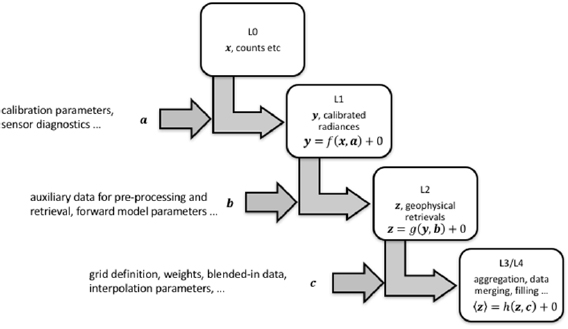
Figure 2. Relationship of satellite data processing levels from level 0 to 3+. In each transformation, data from the lower level ( ,
,  ,
,  ) are transformed to the next level by a function (or process;
  ,
,  ,
,  ).The transformation function or process uses the lower-level data plus auxiliary parameters and data (
 ,
, ,
,  ). In each transformation, uncertainty in lower-level data propagates to the higher level. The auxiliary parameters, data and the assumptions implicit in the function/process (represented by '+ 0') introduce new sources of uncertainty. Some aspects of the transformation may reduce uncertainty, e.g. in averaging over values subject to independent errors.
Download figure:
Standard image High-resolution imageTo our knowledge, no complete, traceable analysis and propagation of uncertainty from L0 or L1 to L2, L3 or L4 exists for any current EO processing chain.
Since a classic concern of laboratory-based metrology is to trace measurements to SI standards with a stated uncertainty, we need to address the role of SI standards in satellite measurements. SI-traceable reference standards have not yet been established in orbit (although concepts have been proposed to bring in-orbit SI traceability to future EO missions (e.g. Fox et al (2011) and Topham et al (2015)). Because of this currently sensors are characterised and data are validated by sensor calibration systems (e.g. reference sources or reflectors that have been characterised pre-flight) and in situ measurements (e.g. ground measurements of geophysical quantities that can be compared with those derived from satellite EO measurements). Even where sensor calibration systems have been characterised pre-flight in a fully SI traceable manner, traceability in orbit is compromised by the stresses of launch, the operation of sensors in the harsh environment of space, and the degradation of sensor components over time. On-the-ground validation data for geophysical quantities retrieved from EO measurements also often do not have established SI-traceability, although some agencies are now investing in fiducial reference measurements (Thorne et al 2018) to support the Copernicus space programme in particular. SI-traceability for reflectance is being developed within the instrumented calibration network, RadCalNet (www.radcalnet.org). For EO-derived sea surface temperature (SST), there are efforts towards SI-traceable at-surface references for radiometric SST using ship-borne radiometers (FRM4STS http://www.frm4sts.org/). For atmospheric variables, the GRUAN (GCOS reference upper air network) provides observations traceable to a SI unit or an internationally accepted standard (Bodeker et al 2016).
Even where SI-traceability is being established via ground truth, uncertainty in that traceability chain may be larger than desirable for applications such as climate research. Other challenges include accounting for differences between what the ground instrument is measuring and what the satellite measures, which can include problems of scale of sampling ('point-to-pixel' effects) and differences in the detailed meaning of the measurand between satellite and in situ systems.
What, then, is the relevance of metrology to historical Earth observations obtained in the absence of SI traceability either in orbit or on the ground? Historical sensors provide critical information of the state of the planet during a period of relatively rapid climatic change. Even without full SI-traceability, there is a key role for metrology to work with EO practitioners towards rigorous characterisation of measurement errors, so that a historic EO dataset can be used appropriately for science in the light of well-understood uncertainty and stability estimates. Establishing the stability of an EO time series in relation to a community-agreed reference is a crucial and essentially metrological task in support of defensible interpretation of observed long-term change. This process can lead to an improved post-calibration of historical sensors as the metrological review provides new insight to the physical processes on the sensor.
3. Uncertainty analysis for Earth observation
3.1. Introductory comments on metrology
The metrological community, through the Metre Convention and the international system of units (SI), has achieved century-long stability and international consistency of measurement through key principles of traceability: uncertainty analysis and comparison.
Metrological traceability is a property of a measurement that relates the measured value to a reference through an unbroken chain of calibrations or comparisons. Uncertainty analysis is the review of all sources of uncertainty and the propagation of those uncertainties through the traceability chain. Traceability and uncertainty analysis at National Metrology Institutes (NMIs) are rigorously audited through the Mutual Recognition Arrangement (Comité international des poids et mesures 1999), which involves formal international comparisons.
Here we consider selected core principles of metrology and how they apply to EO. It should be noted here that these core principles form the basis of the QA4EO framework endorsed by CEOS in 2010 and in this paper we expand on this guidance to provide more detailed practical examples of implementation and in doing so extend the concepts to address some specific EO issues.
Key Uncertainty Concepts for EO
3.1.1. Error, uncertainty, effect.
The Guide to the Expression of Uncertainty in Measurement (GUM 2008; hereafter 'the GUM'), and its supplements provide guidance on how to express, determine, combine and propagate uncertainty. The GUM and its supplements are maintained by the JCGM (Joint Committee for Guides in Metrology), a joint committee of all the relevant standards organisations and the International Bureau of Weights and Measures, the BIPM.
The GUM defines the uncertainty of measurement as a:
parameter, associated with the result of a measurement, that characterizes the dispersion of the values that could reasonably be attributed to the measurand.
Uncertainty is non-negative. The 'standard uncertainty' is the measurement uncertainty expressed as a standard deviation. Evaluations of uncertainty in this paper refer throughout to standard uncertainty.
The error of measurement is defined in the GUM (section 2.2.19) as the:
result of a measurement minus a true value of the measurand
Since the true value of the measurand is unknown, the measurement error is unknown. However, by analysing the sources of errors in an EO measurement, the uncertainty in the measured value can be evaluated. This is the topic of section 3.2 below.
Estimating the uncertainty involves complex considerations, because any measurement is subject to several different sources of error, or 'effects'. The approach to uncertainty analysis presented below is to evaluate the uncertainty arising from different effects and combine these to determine the uncertainty associated with a measured value.
3.1.2. Independent, structured and common errors, correlation.
The measured value in each pixel of an EO image is the result of a sequence of steps and transformations. In transforming from raw data (L0) to calibrated radiances (L1), many measured values relevant to calibration measurements may be combined. In transforming L1 radiances to L2 geophysical products (figure 2), radiances from different spectral bands may be used. In L2 to L3 + processing, data across different pixels are then combined. Where correlation exists between errors in different measured values (different wavelengths and/or pixels), this error correlation needs to be considered in the uncertainty analysis.
The GUM defines systematic and random errors, concepts that are widely used in science.
Random errors are errors manifesting independence: the error in one instance is in no way predictable from knowledge of the error in another instance. A complication arises in EO imagery when one instance of a parameter in the radiance measurement function is used in the calculation of the Earth radiance across many pixels. That component of the error in the radiance image is then correlated across pixels, even though the originating effect is random. Put another way, the originating random error contributes errors with a particular structure to the image.
Systematic errors are those that could in principle be corrected for if we had sufficient information to do so: that is, they arise from unknowns that could in principle be estimated rather than from chance processes. All systematic errors in EO are structured in that there is a pattern of influence on multiple data. They include, but are not limited to, effects that are constant for a significant proportion of a satellite mission—i.e. biases, for which the structure is a simple error in common.
When considering EO imagery, it is can be useful to categorise effects primarily according to their cross-pixel error correlation properties, as independent, structured or common effects.
3.1.2.1. Independent errors.
Independent errors arise from random effects causing errors that manifest independence between pixels, such that the error in  is in no way predictable from knowledge of the error in
  , were that knowledge available. Independent errors therefore arise from random effects operating on a pixel level, the classic example being detector noise.
3.1.2.2. Structured errors.
Structured errors arise from effects that influence more than one measured value in the satellite image, but are not in common across the whole image. The originating effect may be random or systematic (and acting on a subset of pixels), but in either case the resulting errors are not independent, and may even be perfectly correlated across the affected pixels. Since the sensitivity of different pixels/channels to the originating effect may differ, even if there is perfect error correlation, the error (and associated uncertainty) in the measured radiance can differ in magnitude. Structured errors are therefore complex, and, at the same time, important to understand, because their error correlation properties affect how uncertainty propagates to higher-level data.
3.1.2.3. Common errors.
Common errors are constant (or nearly so) across the satellite image, and may be shared across the measured radiances for a significant proportion of a satellite mission. Common errors might typically be referred to as biases in the measured radiances. Effects such as the progressive degradation of a sensor operating in space mean that such biases may slowly change.
3.1.2.4. Notes on usage of 'error' and 'uncertainty'.
In this section, we have classified the effects by the correlation structure of the errors they cause. Since uncertainty describes the dispersion of errors, and not the nature of the errors, uncertainty should not be described as random, systematic, independent, etc. Metrologists generally use phrases such as 'the uncertainty associated with random effects' rather than 'random uncertainty'.
Some metrologists avoid the word 'error' to avoid the confusion arising from incorrect usage of 'error' and 'uncertainty' in much scientific literature. There is often no ambiguity in the case of a repeated measurements in a laboratory, where the dispersion in measured values arises solely from the dispersion of measurement errors. But, in EO, it is essential to distinguish the dispersion in measured radiances due to geophysical variability (signals of interest) from the dispersion due to measurement errors. To maintain that distinction, we find it necessary to use terms such as 'error correlation' and 'error covariance' intentionally and consistently.
3.2. Uncertainty analysis
3.2.1. Overview.
Uncertainty analysis in the GUM begins with modelling the measurement, i.e. linking the measurand to the input quantities from which it is derived. A generic measurement model for a L1 radiance would be

where:  are input quantities; A is the vector of calibration parameters (which are also input quantities but are usefully distinguished); and
  is an input quantity introduced to represent any inadequacy of the function f to represent all phenomena that affect the measurand.
The equations, such as equation (3.1), used to populate L1 products, evaluate the measurand (radiance) using estimates of the input quantities. In the GUM, the convention is for estimates to be represented with the lower-case characters corresponding to the quantities written in upper case. Equation (2.1) is then seen as a particular case of the expression by which the measurand is estimated:

where the input estimates include the recorded sensor counts, etc. This clarifies the meaning of the ' + 0' term previously introduced: 0 is our best estimate of  , which is the expectation of
  (assuming we are using the best measurement model we can formulate).
The uncertainty in the measured value is derived from the evaluation of the uncertainty in each input estimate (or, strictly, from the distribution of possible values of  given
given  ). The uncertainty in all input estimates, including calibration parameters and
  is relevant. Evaluation of the uncertainty in
  means propagation through the measurement model of these uncertainties (or, strictly, distributions).
The GUM and its supplements describe both the 'Law of Propagation of Uncertainty' (hereafter, LPU) and Monte Carlo methods of uncertainty propagation.
The LPU propagates standard uncertainties for the input quantities through a locally-linear first-order Taylor series expansion of the measurement function to obtain the standard uncertainty associated with the estimate,  , of the measurand. Higher order approximations can be applied if necessary.
Monte Carlo methods approximate the input probability distributions by finite sets of random draws from those distributions and propagate the sets of input values through the measurement function to obtain a set of output values regarded as random draws from the probability distribution of the measurand. The output values are then analysed statistically, for example to obtain expectation values, standard deviations and error covariances. The measurement function in this case need not be linear nor written algebraically. Steps such as inverse retrievals and iterative processes can be addressed in this way. The input probability distributions can be as complex as needed, and can include distributions for digitised quantities, which are very common in EO, where signals are digitised for on-board recording and transmission to ground.
Monte Carlo methods can provide information about the shape of the output probability distribution for the measurand, deal better with highly non-linear measurement functions and with more complex probability distributions, and can be the only option for models that cannot be written algebraically. However, they are computationally more expensive, which is an important consideration with the very high data volumes of EO.
Often uncertainty analyses will use a combination of Monte Carlo methods and the LPU, for example by using Monte Carlo methods to determine the uncertainty for a particular quantity, which is then used as an input to LPU in a subsequent uncertainty analysis. In this section, we discuss and illustrate the LPU, while acknowledging the role of Monte Carlo methods.
3.2.2. Propagation of uncertainty: single measurand.
The LPU for a single-variable measurand evaluated from  input quantities with values,
 ![${{\boldsymbol{x}}^{{\rm T}}}=~\left[ {{x}_{1}},\ldots {{x}_{{{n}_{j}}}} \right]$](https://content.cld.iop.org/journals/0026-1394/56/3/032002/revision2/metab1705ieqn045.gif) , can be written as
, can be written as

for a generic measurement function of the form  . Here,
 ![${{\boldsymbol{c}}^{{\rm T}}}=[{{c}_{1}},\ldots ,{{c}_{{{n}_{j}}}}]$](https://content.cld.iop.org/journals/0026-1394/56/3/032002/revision2/metab1705ieqn047.gif) contains the sensitivity coefficients of the measurand with respect to the input quantities. The input error covariance matrix,
contains the sensitivity coefficients of the measurand with respect to the input quantities. The input error covariance matrix, ![$ \newcommand{\e}{{\rm e}} \boldsymbol{S}(\boldsymbol{x})=\left[ \begin{array}{@{}cccccccccccccccccccc@{}} {{u}^{2}}\left( {{x}_{1}} \right) & u({{x}_{1}},{{x}_{2}}) & \cdots \\ u({{x}_{2}},{{x}_{1}}) & {{u}^{2}}\left( {{x}_{2}} \right) & \cdots \\ \vdots & \vdots & \ddots \end{array} \right]$](https://content.cld.iop.org/journals/0026-1394/56/3/032002/revision2/metab1705ieqn048.gif) , is square. Each row and each column corresponds to one input quantity. The elements represent the error covariance associated with pairs of input quantities, and, down the diagonal, the error variance (uncertainty squared) of each input quantity.
, is square. Each row and each column corresponds to one input quantity. The elements represent the error covariance associated with pairs of input quantities, and, down the diagonal, the error variance (uncertainty squared) of each input quantity.
The sensitivity coefficients are the first-order derivatives of the measurement function evaluated at the estimates of the input quantities and denoted by  . They can be analytically calculated when the measurement function can formally be differentiated, or can be numerically approximated using finite-difference methods, or can be experimentally determined.
Using the symbol conventions per satellite processing level in figure 2, consider a single-pixel L2 product calculated using a function  which combines measured Earth radiances,
  in
in  spectral channels and uses estimates, b, of the retrieval parameters. Then, the LPU takes the form
  , where
 ![${{\boldsymbol{y}}^{{\rm T}}}=\left[ {{y}_{1}},\ldots {{y}_{{{n}_{c}}}},{{\boldsymbol{b}}^{{\rm T}}} \right]$](https://content.cld.iop.org/journals/0026-1394/56/3/032002/revision2/metab1705ieqn054.gif) . The vector of sensitivity coefficients relates the Earth radiance values in different spectral channels and the retrieval parameters to the retrieved L2 variable (see section 2.2.3):
. The vector of sensitivity coefficients relates the Earth radiance values in different spectral channels and the retrieval parameters to the retrieved L2 variable (see section 2.2.3):
and ![${{\left[ \boldsymbol{S}(\boldsymbol{y}) \right]}_{1,1}}={{u}^{2}}\left( {{y}_{1}} \right)$](https://content.cld.iop.org/journals/0026-1394/56/3/032002/revision2/metab1705ieqn055.gif) ,
, ![${{\left[ \boldsymbol{S}(\boldsymbol{y}) \right]}_{1,2}}=u\left( {{y}_{1}},{{y}_{2}} \right),~$](https://content.cld.iop.org/journals/0026-1394/56/3/032002/revision2/metab1705ieqn056.gif) etc. The derivatives in equation (3.2) are evaluated at the estimates (measured values) of the corresponding input quantities.
etc. The derivatives in equation (3.2) are evaluated at the estimates (measured values) of the corresponding input quantities.
3.2.3. Propagation of uncertainty: multiple measurands.
The LPU can be extended to multiple measurands (output quantities) (GUM-102 2011). Consider the case of retrieval of L2 variables from radiances,  , where Z consists of several geophysical quantities of interest obtained jointly from a common set of multi-channel radiances, Y. The propagated uncertainties associated with values of z are the contents of the following error covariance matrix:

Here,  is the error covariance matrix for the input quantities, expressed in terms of a diagonal matrix of input standard uncertainties, U, and a matrix of error correlation coefficients between input quantities,
 ![$ \newcommand{\e}{{\rm e}} \boldsymbol{R}=\left[ \begin{array}{@{}cccccccccccccccccccc@{}} 1 & {{r}_{1,2}} & \cdots \\ {{r}_{2,1}} & 1 & \cdots \\ \vdots & \vdots & \ddots \end{array} \right]$](https://content.cld.iop.org/journals/0026-1394/56/3/032002/revision2/metab1705ieqn059.gif) . The sensitivity coefficient matrix has elements
. The sensitivity coefficient matrix has elements ![${{\left[ \boldsymbol{C} \right]}_{n,m}}=\frac{\partial {{g}_{n}}}{\partial {{y}_{m}}}$](https://content.cld.iop.org/journals/0026-1394/56/3/032002/revision2/metab1705ieqn060.gif) , i.e.
, i.e.  , evaluated at the estimates of the corresponding input quantities. The output error covariance matrix, S, contains the error covariance of the estimates of the measurands. Even if none of the input terms has correlated errors (and thus R is diagonal), S will generally still be non-diagonal, if (as is likely) the sensitivity matrix includes terms for those output quantities that depend on the same input quantities. A summation of the impact of all error effects is implicit in the summation over all the input quantities.
A subtly different restatement of the LPU will prove useful in section 3.3, where the contribution to the overall error covariance matrix will be calculated one-effect-at-a-time and then summed over the effects explicitly. This approach will be adopted for considering the error covariances between different pixels in an image and between different channels at a given pixel location. This situation differs from the multiple-measurand case above in that now each pixel/channel radiance (output value) is the same function of its own set of input values—i.e. ![${{\boldsymbol{y}}^{{\rm T}}}=\left[\,f\left( {{\boldsymbol{x}}_{1}} \right),f\left( {{\boldsymbol{x}}_{2}} \right),\ldots \right]$](https://content.cld.iop.org/journals/0026-1394/56/3/032002/revision2/metab1705ieqn062.gif) . In this case,
. In this case, ![${{\left[ \boldsymbol{C} \right]}_{n,m}}=0$](https://content.cld.iop.org/journals/0026-1394/56/3/032002/revision2/metab1705ieqn063.gif) for
for  , and C is square and diagonal. For a single effect,
  , applying to measurement function term,
  , the contributed error covariance is
  . This looks the same as equation (3.5), but the meanings and structures of the matrices are a particular case. These points will be explained more fully below.
3.3. Uncertainty analysis at Level 1
3.3.1. Hierarchical structure of error effects.
The uncertainty analysis we describe here is centred on the measurement function for calibrated radiances, the data of L1 products. Typically, some input quantities are directly determined (by measurement, parameterisation or data analysis), while others are determined through their own measurement function of other input quantities. Thus, there can be a hierarchical aspect to uncertainty analysis. To help organise a measurement-function centred analysis of uncertainty, it can be useful to prepare a graphical representation in the form of an uncertainty analysis diagram (figure 3).

Figure 3. Uncertainty analysis diagram: hypothetical case for a measurement function  , where the input quantities, the
  are metrologically independent (have no common error). There are three identified effects that cause uncertainty in the first measurement function term,
  . The contribution to uncertainty and error correlation (from spectral band to spectral band and/or from image pixel to image pixel) properties for each of these effects have been evaluated and encapsulated in a quantitative model for each effect, these models being indicated symbolically by
  , etc. The uncertainty in
  propagates to the measurand via the sensitivity coefficient
  . The second term is itself the result of an explicitly-calculated measurement function, meaning that the analysis is hierarchical. Two effects operating on different terms cause uncertainty in
  . The propagation of uncertainty
  , for example, to the measurand is via a sensitivity obtained by the chain-rule of sensitivity coefficients along the connecting branches:
  . Three identifiable physical effects contribute to the uncertainty
  , but these cannot be separately quantified. Instead, they are jointly evaluated in terms of their combined uncertainty and error correlation properties, and treated in calculation of propagated uncertainty as the single effect
  . Lastly,
  represents the fact that the form of the measurement function itself embodies assumptions and approximations that cause uncertainty in the measurand that should be evaluated.
Download figure:
Standard image High-resolution imageWe find that most radiance measurement function terms are sensitive to one or more effects, and the uncertainty due to each effect needs to be estimated. Quantities not subject to effects include mathematical and physical constants, and agreed reference quantities. In some cases, contributing effects may be estimated separately and then combined, and in other cases, all the effects operative on a single quantity may only be jointly estimated. Many effects are possible in EO: examples at L1 include detector noise, temperature gradients across reference targets, stray light ingress and temperature sensitivity of electronics. The '+ 0' term in a radiance measurement function represents effects relating to the assumptions underlying the form of the measurement function, e.g. that the sensor response is linear or quadratic in underlying radiance. Example effects for a particular sensor are discussed in section 4. Uncertainty analysis starts at the terminations of the uncertainty analysis diagram and propagates uncertainty through each measurement function, in sequence through the hierarchy as necessary.
Uncertainty analysis presumes that the result of a measurement has been corrected for all recognized systematic effects, and that every effort has been made to identify such effects (GUM 2008 section 3.2.4). This means that the measurand will be as accurate as possible given the current state of knowledge. When we perform analyses at the effects level we need to decide whether the effect could be fully, or partially corrected for, and if so we should apply the correction. The residual uncertainty after correction is smaller. Performing uncertainty analysis therefore often has the co-benefit of improving EO data.
3.3.2. Correlation of effects.
Each effect causes uncertainty, meaning it gives rise to an unknown error in each measured value of radiance. Errors may be independent, in common, or have intermediate degrees of correlation. Three different forms of correlation need to be understood to characterise L1 uncertainty for users:
- The error correlation between different quantities in the measurement function. Such error correlations arise from effects in common between different quantities in the measurement function, and where quantities are determined from a common fit to data.
- The error correlation between image pixels for a given spectral band, which may arise when different image pixels have used some of the same input data in the calculation.
- The error correlation between spectral bands for a given pixel, which may arise when different image pixels have used some of the same input data in the calculation.
It is advantageous for uncertainty analysis to formulate the measurement function to avoid the first form of correlation, so that effects are defined by construction to be independent. The LPU can then be expressed as a sum of covariance matrices over effects. Effect independence can be achieved by using hierarchical analysis to pre-combine terms that have a common error component. For example, consider calculation of a reflectance value that depends on the satellite view angle. The satellite view angle may be calculated from longitude and latitude values, both of which are sensitive to a common time error. We can construct the measurement function in terms of the satellite view angle and consider the effect of time error on that angle. A second example arises when there is error covariance between empirical calibration parameters that were obtained in a joint fitting procedure. We can treat these parameters as a single, vector input quantity, and handle the error correlation using their estimated error covariance.
Error correlation between pixels and spectral bands also arises from errors in common. It is important to distinguish 'common effects' from 'common errors'. The same effect might be present in multiple measurements (for example, all measured radiances will be sensitive to noise), but a common error only arises if the same instance (value) of a quantity is used. Earth-view radiances in an image come from different measurements for each channel and pixel, and therefore a different error instance in each radiance. In contrast, a single view of an on-board calibration target may be used to calibrate several lines of pixels, and therefore there is a common error instance for all those pixels. Similarly, any error in characterising the temperature of a black-body calibration target affects all the calibrated thermal channels.
3.3.3. Calculation of error covariance for L1.
Since our uncertainty analysis is based on metrologically-independent effects by construction of the measurement function, we can find the error covariance matrix for a vector of Earth radiance values (e.g. radiance values for different spectral channels and/or for different image pixels) as a sum over effect-specific error covariance matrices:
This is written as a sum over input quantities,  , in the measurement model. The sum is over the associated effects,
  , i.e.
  given
given  . We write it this way to make explicit that there may be multiple effects for a given input quantity, although, since effects influence only one quantity by construction, we could simply sum over effects. The sensitivity coefficient matrix,
  , is diagonal, because each radiance is separately determined from its own evaluation of its measurement model and any quantities in common are addressed in the correlation matrix (see below). Each row/column refers to one corresponding radiance in the vector measurand (i.e. per spectral band or per image pixel). The units of the sensitivity coefficient are the units of radiance divided by the units of the input quantity,
  , and the derivatives are evaluated at the estimate of the quantity.
The uncertainty matrix  is a diagonal matrix of the same dimension, with the standard uncertainty associated with the effect down the diagonal. These uncertainties are in the units of the input quantity, j .
The correlation coefficient matrix  shows the error correlation for the effect
  between the evaluations of the measurement function for the different radiances. Typically, all the radiances have the same form of measurement function, with the same terms. Some of these terms have an independent value for each evaluation of radiance, as when each radiance is estimated from the corresponding Earth counts. In this case, there is no correlation, and
  is the identity matrix. Other terms may have the same value for each evaluation of radiance, in which case
  is the matrix of ones. In more complex cases, terms may have different values whose errors are neither fully correlated nor uncorrelated, in which case
  will have a complex, non-diagonal form.
We choose to decompose the error covariance matrix for the term into uncertainty and correlation matrices,  , because correlation structures are often fixed even if uncertainty varies. Not all effects lend themselves to this treatment, and in such cases the error covariance matrix,
  , may be better evaluated directly. In this case, the contribution to the error covariance matrix for that effect would be
  .
.
The description above has considered a general set of radiances constituting a vector measurand. Typically, we are interested in one of three specific cases: radiance values across the elements of a line for a particular channel; radiance values across the lines for a particular element in a particular channel; and radiance values for a given pixel (line and element) across the channels measured by the sensor. In the first case, the result is the cross-element error covariance matrix for the given channel,  . In the second case, it is the cross-line error covariance matrix,
  . The third case gives the cross-channel error covariance matrix,
  . The indices in this notation operate as follows. The subscript indicates the dimension across which the error covariances are calculated: thus the cross-channel matrix has subscript,
  , for example. The superscript indicates a dimension that is not averaged across. Thus, the cross-element error covariance is evaluated for a particular line,
  . Since it would never make sense to average error covariance matrices across channels, there is no need to have
  in the superscript: that is implicit. To calculate a cross-element error covariance matrix representative of many lines in an image,
  , we would need to evaluate
  for many different lines, and then average these. Denoting by
  the average of
  over an adequate set of lines,
  . Further,
  indicates that a cross-channel error covariance matrix is calculated at a particular pixel,
  . Such a notation is required because there are many possible covariance matrices that can be calculated and used, and they need to be uniquely indexed.
To make this description more concrete we can consider the cross-channel error covariance matrix calculation for a three-channel sensor subject to two effects. Let the first effect,  , be fully correlated, because a common value,
  , is used in the calculation of all three channel radiances.
  might quantify the state of a common calibration target, for example. Then, evaluating at a pixel,
  , we have:
This fully correlated effect ( , the all-ones matrix) has the same uncertainty for each channel, but differing sensitivity coefficients. An effect,
  , that has no correlation between channels, would have a correlation matrix
  . In that case the uncertainty may be different for each channel: the values of the equivalent term in the measurement function for each channel may be separately quantified, with a different uncertainty in each case. A cross-channel error covariance that is representative for many pixels in an image could be calculated as:

Analogous steps would be necessary to find the error covariance matrix for Earth radiance values obtained in different spatial pixels, such as across the elements of a line. The matrices in that case would have a dimension equal to the number of pixels of interest. The correlation coefficient matrix for a single effect,  , would represent the correlation coefficients between the errors in a particular term across that set of pixels.
3.4. Practical aids to uncertainty analysis
3.4.1. The uncertainty analysis diagram.
We previously introduced (section 3.3.1) the uncertainty analysis diagram, in order graphically to illustrate (i) that uncertainty analysis may have a hierarchical aspect, and (ii) the different paths by which effects may influence the measurand. The measurement function is centrally placed in the uncertainty analysis diagram, and the analysis of EO we present here is likewise 'measurement-function centred'. The uncertainty analysis diagram is an aid to the organisation and documentation of metrologically traceable measurement-function centred uncertainty analysis of complex EO sensors. For each term of the measurement function, the origin of uncertainties is identified. On the branches of the diagram, the sensitivity coefficients are placed that relate the uncertainty in terms of the uncertainties in the measured values. The end points of the diagram identify the complete set of effects analysed.
There are choices about how the uncertainty propagation is in practice to be calculated, and these choices are reflected in the structuring of the uncertainty analysis diagram. Careful thought is needed to balance the need for an understandable measurement function while avoiding too many hierarchical levels of measurement function and constructing each effect as metrologically independent (section 3.3.1). In documentation and in the processing code, it is necessary to record the origin of each term in the measurement function and the data used in processing.
3.4.2. Effects tables.
Each effect requires several aspects to be quantified and documented. A useful aid to organising this effort is to synthesise the knowledge of each effect in its own 'effects table'. The effects table records the information needed about this effect to perform a full uncertainty analysis and propagation calculations. An effects table suitable for EO metrology is shown as table 2.
Table 2. Table for codifying the correlation structure in L1 radiances.
| Table descriptor | How this is codified | Notes | |
|---|---|---|---|
| Name of effect | A name for each source of error | Names should be unique | |
| Measurement function term affected | Name and standard symbol of affected term | Usually an effect will only affect a single term, by construction | |
| Instruments in the series affected | Identifier of the specific sensors/satellite platform for which this effect matters | Some effects may arise only for specific sensors in a series | |
| Correlation type and form | Cross-element | One of a number of error correlation forms arising in EO | Codifies the form of spatio-temporal error correlation, addressing all the relevant dimensions that are relevant. |
| Cross-line | |||
| Between images/orbits | |||
| Over time | |||
| Correlation scale | Cross-element | In units of pixels, lines, time or images/orbits—what is the scale of the correlation form? | The scale parameter has a meaning specific to each correlation form |
| Cross-line | |||
| Between images/orbits | |||
| Over time | |||
| Channels/bands | List of channels/bands affected | Channel names in standard form | Some effects may only affect certain channels |
| Error correlation coefficient matrix | A matrix (or specification to calculate the matrix) | This is  |
|
| Uncertainty | PDF shape | Functional form of estimated error distribution for the term | Often Gaussian, or rectangular |
| Units | Units in which PDF shape is expressed | Units of term, or can be as percentage etc | |
| Magnitude | Dispersion of PDF as standard uncertainty | May point to data quantifying uncertainty per pixel/channel | |
| Sensitivity coefficient | Value(s) or equation for of sensitivity of measurand to term | Yields measurand units when multiplied with term standard uncertainty | |
First, the table documents uniquely the name of the source of error and which term is affected. Even within a series of nominally similar sensors, a particular effect may not arise in every case, so the affected sensors must be identified.
Next, the functional dependence ('form') of spatio-temporal error correlation is codified. The form of error correlation must be characterised across several 'dimensions': between elements, between lines, between images/orbits and over time. If correlation does not arise over one of these dimensions, the corresponding correlation form is recorded as independent for the given effect. Across a dimension where correlation does arise, the error correlation structure can take various forms, depending on the origin of the common component of error. For example, there will be an uncertainty associated with the measurement of an on-board calibration target. On-board calibration may be performed at intervals, meaning that the error in calibration result affects all lines observed between calibration cycles. The error correlation then has a rectangular form, being 1 for the lines that use that calibration result, and 0 for lines prior and after that refer to the result of an independent calibration cycle. If the calibration results are smoothed using a boxcar running average over several calibration cycles, which introduces a triangular form of error correlation.
Several forms of error correlation arise often in EO, and in the effects table we use defined names (e.g. rectangular, triangular, bell-shaped) to refer to these. A correlation scale parameter is defined for each of these forms that specifies the range of elements, lines, images or time over which the error correlation is non-zero.
The effects table then characterises the error across channels, specifying the cross-channel correlation matrix, which is often either I or J, as discussed in section 3.3.3.
The estimated shape and dispersion of the error distribution are tabulated next. The uncertainty may be as simple as a constant per channel for a given effect, or may be specified by an equation or parameterisation, or may be a layer of data per pixel per channel. The same may be true of the sensitivity coefficients.
3.4.3. Uncertainty and sensitivity estimation.
Various methods are available for estimating uncertainties and sensitivity coefficients.
Uncertainty can be evaluated from the standard deviation or the Allan deviation (Allan 1966) of repeated measured values, where available. Uncertainty may also be evaluated using simulation, the results of pre-flight tests, or characterised behaviour of similar instruments. Particularly for historical satellite sensors, we may not have all the information ideally needed, so pragmatic estimates must be made.
Where there is an analytic measurement function, a sensitivity coefficient is most easily determined as its partial derivative. Where it is not possible to evaluate a partial derivative, sensitivity coefficients can be determined through perturbation of the values of the inputs of a software function, or from experimental (e.g. pre-flight) data, for example that showing the sensitivity of the instrument gain to temperature.
3.5. Uncertainty characterisation at higher product levels
Once uncertainty and error correlation are characterised at L1, the information should inform the retrieval of geophysical quantities at L2, and formation of L3 and L4 products. In present practice, however, in the absence of propagatable uncertainty information at L1, uncertainty characterisation at higher levels often relies on comparisons between products or validation campaigns.
Given L1 uncertainty information, it becomes possible to propagate radiance uncertainty through the retrieval algorithm to the L2 product. For a single-pixel, multi-channel retrieval,  , this may be feasible analytically using the LPU and the cross-channel error covariance matrix,
  , where the sensitivity coefficients are of form
  . Alternatively, a Monte Carlo approach drawing from the distribution described by
  can be used.
Retrieval also introduces uncertainty. If the inversion process uses data,  , in addition to the radiances, then errors in these data also propagate into retrieval errors. Additional data may include parameters of the retrieval and simulated radiances. Retrieval also is often irreducibly ambiguous. This arises when radiances that are indistinguishable to within their uncertainties can result from a range of geophysical states. This does not imply the radiances are useless: if the distribution of geophysical states that are plausible for a given set of radiances is narrower than the natural variability of the state, the retrieval is informative. Retrieval methods in EO typically select one plausible state given the radiances as the best estimate, this choice arising either implicitly or explicitly from additional constraining information within the retrieval method. The error from collapsing this ambiguity on to the best estimate tends to be correlated in space and time, with a distinct local correlation structure. In atmospheric sounding (retrieval of vertical profiles of atmospheric properties), it is well understood that radiances carry limited information about vertical structure, and the ambiguity is quantified (e.g. Rogers (2000)) as 'smoothing error' (sic). In another example, simulation has been used to characterise the spatio-temporal correlation of errors in retrieved sea surface temperature (e.g. Merchant and Embury (2014)).
For gridded products (L3) spatio-temporal error correlation affects the uncertainty. While noise in the per-pixel retrieved values tends to average out during gridding, uncertainty from errors with significant spatio-temporal error correlation reduces less. Given knowledge of the spatio-temporal error covariance matrix for the pixels involved in the grid average, the uncertainty from averaging (equation (2.3)) can of course be quantified using the LPU, at least in principle. Some users of EO data, such as climate modellers, required quite large-scale averages of data (say, an average of all the retrieved values within a 1102 km2 area—i.e. 1° by 1° at the equator—obtained over the course of a month). Full evaluation of the uncertainty in such a case could imply an infeasibly large calculation, and more research is needed into widely applicable approximate methods.
4. An example metrological analysis
4.1. Introductory context
To make the concepts and discussion in previous sections more concrete, we present an example tracing the uncertainty in estimating sea surface temperature (SST) data from observations taken from the advanced very high resolution radiometer (AVHRR). We start by looking at the calibration of the AVHRR to understand all source of uncertainty in the observed radiances and give some selected effects as examples. Using a simple simulation we then add in some extra sources of uncertainty related to the SST retrieval algorithm to show some of the steps needed in generating uncertainties at Level 2.
4.2. The AVHRR instrument
4.2.1. Overview.
EO missions are typically described by a set of documentation. To undertake a metrological analysis of a historical EO sensor, the available documentation should be used to understand the sensor operation, including hardware and procedures for in-flight calibration, as illustrated for AVHRR below.
In the IR, the AVHRR uses two different types of solid state detector. An InSb detector is used for its 3.7 µm channel, which has a close-to-linear response apart from minor circuit non-linearity. The HgCdTe detectors used for the 11 µm and 12 µm channels have a distinct non-linear response. The AVHRR on-board calibration system uses an internal calibration target which has a quoted emissivity of 0.985 140. Note that this emissivity value is purely theoretical and is considered to be significantly more uncertain than implied by the number of significant figures quoted. Its value is, however, known to be significantly less than 1, since reflected components (proportional to 1 minus emissivity) are seen in the calibration signal, including solar contamination (e.g. Cao et al (2004)).
The AVHRR is a scanning radiometer that collects images as a sequence of scan lines at right angles to the direction of travel of the satellite over the ground. The in-flight calibration procedure makes ten measurements (as counts) per scan line when viewing the internal calibration target (ICT) and ten measurements per scan line of a space view. Four platinum resistance thermometers (PRTs) measure the temperature of the ICT and allow an estimate of the spectral radiance of the ICT to be made, using Planck's Law and the quoted emissivity. From the spectral radiance, the channel-integrated spectral radiance (usually referred to as simply 'radiance') of the ICT is calculated by integrating spectral radiance across the (assumed known) spectral response function (SRF) of a given channel. This ICT radiance coupled with the counts for the ICT and space-view enable the instrument gain to be estimated. The gain is combined with other calibration parameters to convert the counts observed when looking at the Earth into Earth-view radiance. Radiance is often then expressed as brightness temperature, by inverting the channel-integrated Planck function numerically.
The calibration algorithms of the AVHRR have evolved during the series of missions from 1978 to present. Originally, no account was made for the non-linearity of the 11 µm and 12 µm HgCdTe detectors. Subsequent calibration schemes used a range of look-up tables or correction terms for this non-linearity. The current operational calibration is based on Walton et al (1998) and involves calculation of a linear radiance which is then corrected using a quadratic correction. This formulation is intrinsically problematic (Mittaz et al 2009). Further, using parameters derived from pre-launch data within this formulation gives rise to significant biases (Wang and Cao 2008, Mittaz and Harris 2011).
An improved radiance measurement function, modified from Mittaz and Harris (2011), is:
where  is the Earth radiance,
  is the estimated radiance of the ICT,
  is the counts observed when looking at the ICT averaged over a number of scanlines (in practice a space-view count Cs minus a target count) and
  is the Earth-view count (in practice a space-view count minus the Earth-view count) and
  are calibration parameters that have physical interpretations. We assume that this quadratic form represents the non-linearity adequately though this will be discussed in section 4.2.5. For the AVHRR the dark, space-view count, is set to be higher than the signal count for operational reasons.
4.2.2. An uncertainty analysis diagram for the AVHRR.
An uncertainty analysis diagram for the AVHRR measurement function is shown in figure 4. It shows the sources of uncertainty from their origin (shown on the outside portions of the diagram) through to the uncertainty in the final measurand. The sources of uncertainty range from independent effects with a physical origin, such as detector noise sources, to structured effects associated with the estimate of the internal calibration target (ICT) radiance to common effects related to the harmonisation process. A full discussion of all effects is beyond the scope of this paper, and this complete diagram is included mainly to illustrate the scale of a full uncertainty analysis for a relatively simple instrument. At the stage of constructing an uncertainty analysis diagram, it is also best practice to include all potential sources of uncertainty, even those suspected to be negligible. For a metrologically-traceable uncertainty estimate, the neglect of any contributing term should be justified and documented.
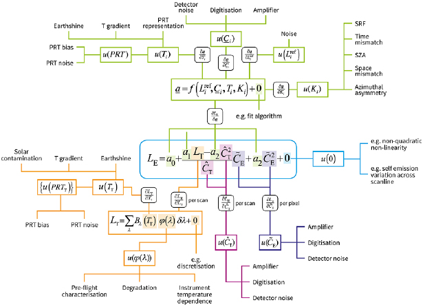
Figure 4. Uncertainty analysis diagram for the AVHRR. The AVHRR infrared radiance measurement function is an analytic equation in terms of observed counts and calibration parameters, shown at the centre of the diagram. Each term is addressed by a colour-coded branch that links to an uncertainty model, u(.), for that term that derives from one or more effects, that are noted in the next level of branching. In two cases (namely, the calibration parameter vector a and the calibration-target radiance  ), the term is linked to a secondary measurement function. Links between a term and its uncertainty are labelled with the sensitivity coefficient required to assess the impact of uncertainty in that term to the outcome of the measurement function.
Download figure:
Standard image High-resolution imageNote also that the diagram includes some intermediate processes that themselves contribute to the total uncertainty budget. For example, the ICT radiance is derived from measurements of the ICT temperature from four PRTs. The uncertainty in the ICT radiance is a combination of the uncertainty in the ICT temperature (affected by PRT noise, PRT bias, digitisation and the representativity of this measurement to the ICT temperature seen by the detector, and the issue of thermal gradients across the ICT), uncertainty in the spectral response function, and approximations from use of look-up tables in conversions ('discretisation'). The ICT radiance is also a source of cross-channel error correlations, because the same ICT temperature is used to calibrate all three IR channels and therefore any error will be common to all channels.
In the upper half of the diagram are the components related to harmonisation. Harmonisation involves the re-estimation of the calibration parameters for consistency across the satellite series by using sensor-to-sensor collocated observations ('matches'). Many of the sources of uncertainty listed here are repeated from the lower portion of the diagram, because the harmonisation fit depends on a set of measured counts, each subject to the same effects. The matches have their own uncertainties associated with the quality of the collocation. A detailed analysis of uncertainties in sensor-to-sensor matches has been undertaken by Hewison (2013).
The diagram also includes the sensitivity coefficients on each branch that enable the source uncertainties to be propagated to the measurand.
The uncertainty analysis diagram documents in a visual form the full set of error effects to be analysed and their connections to the measurement function. For each effect represented on the diagram, we use an effects table (section 3.4.2) to aid analysis and documentation.
In the following sections we use specific examples to illustrate the use of the effect tables and consider effects including noise in the space-view counts (Cs), uncertainties in the estimation of the calibration target temperature and the uncertainty due to imperfect characterisation of the HgCdTe detectors (which is an uncertainty associated with the term '+ 0' of the radiance measurement function). The 'counts' example illustrates structured errors, the ICT temperature example illustrates channel-to-channel errors and the 'non-quadratic' example illustrates the metrological principle that effects need to be considered even when there is no direct way of quantifying them.
4.2.3. Space-view counts uncertainty.
Uncertainty in the space-view counts can be derived from the telemetry stored in the AVHRR Level 1b file. Error correlation arises because, as is commonly done in EO, the space-view counts are averaged over a number of scanlines to reduce noise in the calibration values. Table 3 is the corresponding effects table.
Table 3. Effects table for noise in space view counts.
| Table descriptor | How this is codified | |
|---|---|---|
| Name of effect | Space view count uncertainty | |
| Affected term in measurement function | Space view count ( ) ) |
|
| Channels/bands | Channel 3B, 4 and 5 (3.7 µm, 11 µm and 12 µm) | |
| Correlation type and form | Within scanline (pixels) | Rectangular absolute |
| From scanline to scanline (scanlines) | Triangular relative | |
| Between images/orbits (orbits) | None | |
| Between channels/bands | None | |
| Correlation scale | Within scanline (pixels) | (−∞, +∞) |
| From scanline to scanline (scanlines) | (−N, +N) where N is AVHRR dependent | |
| Between images/orbits (orbits) | None | |
| Between channels/bands | None | |
| Uncertainty PDF shape | Gaussian | |
| Uncertainty units | Counts | |
| Uncertainty magnitude | Estimated from Allan deviation from space views accumulated over a complete orbit | |
| Sensitivity coefficient |  |
|
The effects table shows that there are two dimensions of error correlation that have to be dealt with appropriately. First, since the calibration parameters are recalculated each scanline, the space-view counts error is the same for all pixels across a given scanline, and therefore has a correlation of 1 across the whole scanline, which is a 'rectangular absolute' systematic correlation. Note that while the space-view counts error is in common, the sensitivity coefficient differs for the different pixels across the scanline, since the Earth-view count is present in the analytic expression for the derivative. The corresponding radiance errors across the scanline therefore have a predictable structure (determined by the sensitivity coefficient variation) scaled by an unknown random error (since the space counts error is random). Second, because multiple (N) scanlines are averaged to create the calibration coefficients, there is a correlated error in the running-mean space-view counts between scanlines used within the average. The running mean uses a constant weight, and so the form of the correlation is triangular (the correlation decreases for scanlines increasingly far apart) with a base width of ±N scanlines (beyond which the correlation is zero). N varies between different AVHRR sensors and can vary from approximately 20 scanlines up to ~100 scanlines.
4.2.4. Internal calibration target thermal gradient effect.
The measurement function for the AVHRR contains the radiance of the ICT used to calibrate the instantaneous instrument gain. This quantity is itself calculated from the ICT temperature, and that temperature is itself subject to different sources of uncertainty. The ICT radiance is therefore one of the intermediate effects. One of the sources of uncertainty for the ICT radiance is having to estimate the ICT radiant temperature based on temperatures measured at four points only using platinum resistance thermometers attached to the ICT baseplate. The uncertainty then arises because the ICT is subject to large (>1 K), time-variable thermal gradients, so the relationship between the true ICT radiant temperature and these four point temperature measurements is not simple. During the satellite lifetime, the radiant temperature was estimated operationally by the arithmetic mean of the four temperatures. This approach is simple and would give reasonable estimates for an ICT in a well-regulated environment. However, due to the thermal gradients across its surface as well as stray light issues during times of rapid variations in the instrument's thermal state the use of a simple average will lead to significant errors. Figure 5 shows two different sensors, one where this effect is thought to be large (the AVHRR on NOAA-12) and one where it is likely to be small (NOAA-17). Previous studies of this effect on the earlier AVHRRs (e.g. Trishchenko et al (2002)) have commented on the range of variability seen in the PRT measurements (see figure 5) and that these could be used as some kind of broad estimate of the uncertainty on the ICT temperature. This proposed approach cannot be considered as metrologically robust, since it involves no attempt to remove the major source of error.
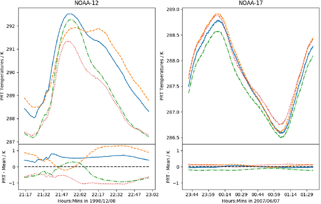
Figure 5. Variation of the four PRT measurements from the AVHRR ICT taken around an orbit. Left: example of NOAA-12 showing significant deviations between the different PRTs implying a strong variation in thermal gradients across the ICT. This implies a large error if the simple mean is used to estimate the ICT temperature. Right: example from NOAA-17 where the four PRT measurements are much closer to each other and where the error in the ICT temperature by taking the mean value of the PRTs will be small, though not negligible.
Download figure:
Standard image High-resolution imageIn a metrological approach, we remove known sources of systematic error (such as errors in the ICT temperature estimate) to the best of our knowledge, and quantify the remaining uncertainty. To do this, we have to consider the process giving rise to the effect (variations in the thermal gradients across the instrument) and how the error will propagate into measured radiances.
Four PRT temperatures are inadequate to determine much detail about the complex thermal gradients across the surface of the ICT. We can, however, exploit understanding of the behaviour of the 3.7 µm channel to constrain the problem. This channel uses an InSb detector which is known to be linear for the radiance levels observed from Earth observation. The 3.7 µm channel gain is therefore expected to be constant around the orbit. We can then reasonably infer that significant deviations from a constant gain reflect errors in the ICT temperature estimate. A direct mapping from gain error to ICT temperature error constrained by the PRT measurements themselves can then be made (full details of the procedure will be published elsewhere). Figure 6 shows data for NOAA-12 from the same orbit as shown in figure 5 (left panel). The left hand plot of figure 6 shows the original and corrected 3.7 µm channel gain. The right-hand plot shows the ICT temperature estimates made using the simple mean of the PRTs (original) and corrected by analysing the 3.7 µm channel gain. The corrected gain has lower variance, suggesting a substantial reduction in the ICT temperature error and the remaining variability in the 3.7 µm channel gain can be used to estimate the ICT temperature uncertainty. The improved ICT temperature can then also be used to calibrate the 11 µm and 12 µm channels, where constant gain is not expected. This metrological approach estimates ICT temperature with reduced systematic errors, and provides a method to evaluate the remaining uncertainty, for propagation to uncertainty in measured radiances.
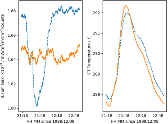
Figure 6. Left: the uncorrected (dashed) and corrected (solid) gain of the 3.7 µm channel as a function of time. Right: operational (dashed) and corrected (solid) estimate of the ICT temperature. The properties of the 3.7 µm channel are such that there should be no gain variation, so the excursion seen in the uncorrected gain (left panel, blue) points to the ICT temperature being mis-estimated (right panel, blue). After applying a method that re-estimates the ICT temperature while minimising the variance of the 3.7 µm channel gain (left panel, orange), the corrected ICT temperature variation (right panel, blue) can be used to remove bias in the other channels (11 and 12 µm) that depend on the ICT temperature for their calibration.
Download figure:
Standard image High-resolution imageThis effect is also one that will introduce channel-to-channel error correlation because any remaining error in the ICT temperature will be present in the calibration of all the infrared channels. This effect has never previously been characterised for the AVHRR. For any given pixel we can use equation (3.7) to estimate a cross-channel error covariance matrix. An example is shown below (table 4) together with the related correlation matrix for a single pixel of NOAA-12. The cross-channel error correlation between the 11 and 12 µm channels is large, and this is significant for retrieval of geophysical quantities using these channels. The effect table for the ICT thermal gradient effect is shown as table 5. We note that currently for the AVHRR one of the table entries (correlation type and form between images/orbits) is labelled as 'Unknown' because we do not currently know what this is apart from a general statement that we might expect close in time orbits to have similar correlation structures and those far apart in time having less correlation. This will be looked at in the future.
Table 4. Correlation and Covariance matrices for a single pixel of NOAA-12 data showing the correlation and covariances introduced by the ICT temperature error effect on the 3.7 µm, 11 µm and 12 µm channels. The unit of the covariance matrix is K2.
| IR channels correlation matrix | IR channels covariance matrix |
|---|---|
 |
 |
Table 5. Effect table for the error in the ICT temperature estimate.
| Table descriptor | How this is codified | |
|---|---|---|
| Name of effect | ICT Temperature Error | |
| Affected term in measurement function |  |
|
| Channels/bands | Channel 3, 4 and 5 (3.7 µm, 11 µm and 12 µm) | |
| Correlation type and form | Within scanline (pixels) | Rectangular absolute systematic |
| From scanline to scanline (scanlines) | Triangular relative systematic | |
| Between images/orbits (orbits) | Unknown at the moment | |
| Between channels/bands | Across the IR channels | |
| Correlation scale | Within scanline (pixels) | (−∞, + ∞) |
| From scanline to scanline (scanlines) | (−N, +N) where N is AVHRR sensor specific | |
| Between images/orbits (orbits) | None | |
| Between channels/bands | None | |
| Uncertainty PDF shape | Gaussian | |
| Uncertainty units | Kelvin | |
| Uncertainty magnitude | Estimated from corrected 3.7 µm channel gain variance | |
| Sensitivity coefficient |  |
|
4.2.5. Detector non-linearity (+0 term).
The effects tables shown as table 6 represent effects related to the assumption that the AVHRR HgCdTe detector can be modelled as a quadratic function of counts with a constant non-linear coefficient. This assumption is built into the AVHRR measurement equation, and therefore any error in this assumption is an effect on the +0 term of the measurement equation. The origin of the non-linearity is dominated by Auger recombination, which is itself related to the lifetime of semiconductor carriers. The exact details of the non-linear behaviour is related to doping levels, lattice defects, etc, in the detector and is not expected to be strictly quadratic. We cannot determine this effect in detail from the pre-launch measurements and do not have access to the original manufacturer's data, and so we cannot directly characterise the errors introduced by the quadratic assumption. So, we must make a Type-B uncertainty estimate, based on expert judgement and independent knowledge. In this case, the latter consists of a numerical model of HgCdTe detectors of the geostationary operational environmental satellite (GOES) Imager (Bicknell 2000). The model determines the Auger recombination lifetimes of the carriers and derives variations in the predicted voltage seen for a given input photon flux. We tuned the model parameters to match the photon fluxes and magnitude of non-linearity seen in the AVHRR sensors. The top two plots of figure 7 shows that the modelled errors in the brightness temperature from approximating the detector behaviour with a quadratic form are of order millikelvin, which is small.
Table 6. Effect table for the assumptions regarding detector non-linearity.
| Table descriptor | How this is codified | |
|---|---|---|
| Name of effect | Non-quadratic non-linearity | |
| Affected term in measurement function | +0 | |
| Channels/bands | Channel 4 and 5 (11 µm and 12 µm) | |
| Correlation type and form | within scanline (pixels) | Rectangular absolute systematic |
| from scanline to scanline (scanlines) | Rectangular absolute systematic | |
| between images/orbits (orbits) | Rectangular absolute systematic | |
| between channels/bands | Rectangular absolute systematic | |
| Correlation scale | within scanline (pixels) | (−∞, +∞) |
| from scanline to scanline (scanlines) | (−∞, +∞) | |
| between images/orbits (orbits) | (−∞, +∞) | |
| between channels/bands | None | |
| Uncertainty PDF shape | Gaussian | |
| Uncertainty units | Radiance | |
| Uncertainty magnitude | Type-B estimate from detector modelling | |
| Sensitivity coefficient |  |
|

Figure 7. Shows the deviation from a quadratic model for an HgCdTe detector for the 11 and 12 µm channels using a theoretical model. This indicates that the deviation from a quadratic are at the milli-Kelvin level.
Download figure:
Standard image High-resolution imageWhile the size of the uncertainties added from the constant quadratic non-linear model used in the measurement equation have been shown to be small compared to other effects, it is important to understand that without the modelling studies undertaken here we would not have a good estimate as to the impact of these particular effect and therefore would not be able to claim metrological traceability in the sense used in this paper. If we had either ignored these effects or not estimated the size of uncertainty in a justifiable manner we would have an incomplete uncertainty model.
4.3. Calculating uncertainties
Once all the effects are described in effect tables, we have the information needed to combine them and estimate the total uncertainty. This can be done analytically or using Monte-Carlo techniques. The analytic methodology has been described in section 3 so here we concentrate on using a Monte-Carlo simulation to understand the properties of the final uncertainties including non-Gaussian effects such as digitisation. We note that this sort of analysis is not the same as that recommended in the GUM appendix 1 but is useful so that the EO community can understand in more detail the underlying distribution of error that is present in their data.
For illustration, we have created a simple model of the AVHRR instrument that includes:
- applicable noise sources (detector noise, PRT noise etc)
- realistic gain variations derived from AVHRR data
- simple thermal gradients across the internal calibration target
- the estimation of calibration parameters over a moving window of ±27 scan lines and realistic digitisation of all instrument data.
We use the AVHRR simulator to simulate the Earth counts and calibration data (space view counts, ICT counts, ICT PRT measurements etc) for a prescribed Earth brightness temperature, which acts as a 'truth'. The simulated instrument values and calibration parameters are used to simulate the errors in the AVHRR measurements, relative to the input 'truth'.
4.3.1. Uncertainties in the AVHRR brightness temperatures including digitisation.
We have simulated AVHRR BTs for one day's worth of full-swath orbital data covering a scene temperature range from 200 K to 300 K and generated at each simulation point 1000 realisations of the simulated 'measured' BT to compare with the 'true' value inputted to the simulation.
Figure 8 shows the simulated error distributions for a cold (200 K) and a hot (300 K) scene for the 11 µm and 12 µm channels. The error distributions are not Gaussian: digitisation causes each distribution to comprise a few separated peaks. The degree of separation depends on the scene temperature because a single count corresponds to a smaller BT increment at higher radiances. This effect is random between pixels, since the detector noise that is digitised is random between pixels. The spread of each peak reflects the effect of the calibration uncertainty, including noise in the calibration measurements.

Figure 8. Traceable, simulated error distributions in AVHRR BTs. Top panels: scene temperature 200 K; bottom panels 300 K. Left panels: 11 µm channel; right panels: 12 µm channel.
Download figure:
Standard image High-resolution image4.4. Uncertainties in sea surface temperature retrievals
To illustrate traceable uncertainties at the geophysical level, we use sea surface temperature retrieval. The basis and current practice of SST retrieval has been reviewed by Merchant (2013); see also the references therein. Typically, SST is estimated from thermal radiances expressed as brightness temperatures, since this significantly linearizes the inversion. Most inversion methods can be reduced to a form  , where
  is the retrieved SST,
  is the brightness temperature of the
  th channel, and the a terms are weights. The weights may be pre-defined coefficients (the traditional approach) or may be calculated dynamically using simulation of the retrieval context using numerical weather prediction fields to give prior information about the state of the surface and atmosphere (a category including various incremental methods, including 'optimal estimation'). Either way, the weights affect the propagation of error from radiance (brightness temperature) to SST. If the radiance uncertainty in the
  th channel is
  and arises from effects that are independent between channels, then the SST uncertainty arising from the radiance uncertainty is
where a generalisation to  channels (rather than just two) is accommodated. This expression is equivalent to the expression in Merchant and Le Borgne (2004), although there it is stated in terms of noise equivalent differential temperature.
Not all errors in the SST retrieval have their origin in radiance errors. Firstly, the inversion of brightness temperature to SST is intrinsically ambiguous to some degree (introducing some uncertainty even if the radiances were perfect—see discussion around section 3.5). Moreover, the inverse, even if unbiased over all, may have limitations in its formulation that lead to effects such as geographical biases. This is the case when coefficient-based approaches are used (Merchant et al 2006). Such retrieval limitations can be quantified by simulation studies where 'perfect' knowledge of SST and of radiances is available (e.g. Merchant et al (2009)). Secondly, the inversion may introduce errors because parameters in the inversion have errors. An example would be simulation (forward model) error in a radiative transfer model used within a physically based retrieval. The uncertainty arising from such effects is harder to estimate. The sensitivity of an inverse method to each parameter can be found by perturbing the parameter and finding the SST impact. However, the uncertainty of each parameter may be unknown and difficult to quantify. Nevertheless, some characterisation of uncertainty arising from the inverse process itself is required within the chain of uncertainty. Other sources of uncertainty can also be present such as sampling biases, regridding errors and correction for diurnal effects.
4.5. A Monte-Carlo simulation of SST retrievals using optimal estimation
Here, we will consider a single SST retrieval algorithm at the pixel level only and use the Monte-Carlo instrument model to obtain simulated 'measured' BTs for 'true' scene temperatures derived from a radiative transfer model (RTM). As in the previous section, this study is using a Monte-Carlo simulation to highlight the likely error distribution in SST rather than doing a GUM based Monte-Carlo uncertainty analysis. We use RTTOV (Saunders et al 1999) version 11.2 with the sea surface emissivity model of Embury et al (2008) as the true physics of radiative transfer. The 'true' state input to this RTM is the SST field of Reynolds et al (2002) together with ECMWF atmospheric profiles obtained from the ERA-Interim dataset (Dee et al 2011). Optimal estimation involves modelled BTs from an RTM and state estimate that are available approximations to the real world. These are represented here by the Community Radiative Transfer Model (CRTM, e.g. Ding et al (2011)) and the Nalli et al (2008) sea surface emissivity model applied to the surface temperature and 26 level profile atmosphere from the National Centers for Environmental Prediction (NCEP). Thus, imperfect knowledge of both environmental conditions and radiation physics are represented.
We then simulate a set of AVHRR orbits using the geolocation and satellite angles/solar angles from real orbits. Only clear-sky pixels are included and we subsample by a factor of ~25 to reduce computation time. The 'observed' simulations provide 1000 realisations of brightness temperatures based on Reynolds/ECMWF/RTTOV plus the AVHRR instrument model. The 'modelled' simulations give the single realisation of BTs from NCEP/CRTM to use in the optimal estimation retrieval. As well as BTs, their derivatives with respect to SST and total column water vapour are also generated.
Optimal estimation (OE) for the AVHRR is described in Merchant et al (2008) and briefly summarised here. In OE, the difference between the satellite observations ('observed') and simulated brightness temperatures ('modelled') assuming a prior state is used to nudge the prior state, giving us the retrieved SST. Uncertainties in both the observed and RTM generated BTs are included via the covariance matrix Se which can also include channel to channel covariances (e.g. section 4.2.4), and for the prior state Sa. K is the matrix of partial derivatives of brightness temperatures with respect to state vector variables. The retrieval algorithm is then written as

where z is the state vector ![$ \newcommand{\e}{{\rm e}} z=\left[ \begin{array}{@{}cccccccccccccccccccc@{}} x \\ w \end{array} \right]$](https://content.cld.iop.org/journals/0026-1394/56/3/032002/revision2/metab1705ieqn142.gif) , in which x is the SST and w is the total column water vapour, and xa is the prior state,
, in which x is the SST and w is the total column water vapour, and xa is the prior state,
Using the 'observed' data we can then derive the distribution of errors expected from an OE retrieval. Figure 9 shows the distribution of the SST obtained from OE retrievals for two different pixels, arising from the 1000 realisations of 'observed' data. The Monte-Carlo approach highlights the influence of digitisation on the error distribution of retrieved products: the most obvious feature of figure 9 is the impact of digitisation propagated to SST, with the distributions being distinctly non-Gaussian and comprising several separated peaks. The mean values of error, associated with the distributions not being centred on zero, arise from errors in the prior information used for the retrieval. The retrieval situations selected show that the propagation of error from the prior can also be significant. Both instrument and retrieval uncertainties both contribute significantly to the final uncertainty in the geophysical product (SST). In laboratory metrology, digitisation is generally not significant, but in EO it can be.

Figure 9. Distribution of the OE retrieval error for two examples of OE retrievals. The distributions are based on 1000 Monte-Carlo simulations where the input noise is from the instrument only.
Download figure:
Standard image High-resolution image
4.6. Remarks
The above results illustrate that metrological approaches are useful for understanding the uncertainties in EO data and that uncertainty information is complex. For AVHRR, digitisation significantly contributes to in total brightness temperature uncertainty; this effect is random, and is not Gaussian. Uncertainty arising in the counts-to-radiance conversion is smaller, but includes structured random and systematic effects. For optimally estimated sea surface temperatures, random effects are smaller than correlated effects associated with the retrieval process, though both are significant. The importance of the structured random and systematic errors propagated to SST will increase when, as is commonly done, creating averaged, gridded sea surface temperature products.
5. Discussion and conclusions
5.1. Aims of EO metrology
The purpose of Earth observation is to quantify the Earth-system in order to understand and live sustainably within the environments of our planet. EO is a measurement science able to provide a legacy of information about the environment and climate of value to science and society.
This paper argues that EO can advance as a measurement science through increased interaction with the discipline of metrology. The potential is not limited to the laboratory-based context of instrument calibration: there is much progress to be made in the formulation and derivation of satellite products informed by metrological principles. Our view derives from experience in applying metrological approaches to historical Earth observations, illustrated by the case study in section 4.
Several metrological principles can inform practice in EO. Perhaps the most basic is that each measured value should be accompanied by meaningful information about its uncertainty. This view has been articulated in relation to climate data records (e.g. Immler et al (2010), Hollmann et al (2013) and Merchant et al (2017)), and is a concept formerly adopted by CEOS via QA4EO. Initiatives in this direction are implemented across the space agencies, at least in connection to current and future missions, but it is not universal practice in EO as a whole and is not widely implemented retrospectively.
A barrier to improved uncertainty information in EO is the absence of pixel-level uncertainty information in level-1 radiance products (with exceptions, e.g. Gorroño et al (2017) for Sentinel-2; or the MODIS uncertainty index see MODIS Level 1B Product User's Guide https://mcst.gsfc.nasa.gov/sites/mcst.gsfc/files/file_attachments/M1054.pdf). All scientific and societal applications follow from the transformation of satellite data from level 1 to higher-level data (figure 2). Each data transformation entails errors propagating from the lower level to the higher and entails new effects that introduce errors. Providing uncertainty estimates for each datum at higher product levels involves a series of uncertainty analyses, and proper propagation of uncertainty through each transformation. Tools to facilitate exploitation of uncertainty information will encourage uptake by users of the data.
Metrology as a discipline provides guidance, principles and tools for uncertainty analysis and propagation. Moreover, the uncertainty estimates provided should be traceable (which ultimately means, scientifically defensible), another aspect where metrological guidance is valuable. The application of metrological principles to EO also needs to be pragmatic, since providing uncertainty information for scientific and practical applications needs to be achieved within certain limitations of resources. Uncertainty analysis in practice will include the prioritisation of the effects that dominate uncertainty on the spatio-temporal scales at which EO data are exploited.
There are relevant concepts in the EO community around improved data and quality (e.g. QA4ECV http://www.qa4ecv.eu). Concepts of the 'fundamental climate data record' (FCDR) and 'climate data record' (CDR) are well established. An FCDR has been defined as 'sensor data (e.g. calibrated radiances, brightness temperatures, radar backscatter) that have been improved and quality controlled over time, together with the ancillary data used to calibrate them'. A CDR has been defined as a time series of measured values of a geophysical quantity of sufficient length, quality and stability to be useful for understanding climate variability and change. The lowest level of satellite product that could comprise a CDR is L2, although products from higher levels of processing are also referred to as CDRs. These definitions have some limitations. Firstly, they are explicitly tied to climate. Climate is a far-reaching application of historic EO data, but not all such archives are developed for climate science or monitoring. Secondly, it is clear in the definition of FCDR that, compared to the original L1 data, the FCDR is improved and quality controlled, but the nature of the improvements are left fairly vague. We take this opportunity to propose an aspirational FCDR definition that is more specific with regards to the intended data properties, as follows:
A fundamental climate data record consists of a long, stabilised record of uncertainty-quantified sensor observations that are calibrated to physical units and located in time and space, together with all ancillary and lower-level instrument data used to calibrate and locate the observations and to estimate uncertainty.
Relative to a straightforward collection of operational L1 data, this definition, firstly, specifies that an FCDR is a stabilised record. An example of steps to stabilise an FCDR is harmonisation (Woolliams et al 2016, Giering et al 2019), which is a process to bring mutual consistency to the radiance calibrations of the sensors in a series, thereby increasing the stability of derived products and minimising artefacts associated with the introduction and retirement of sensors. Harmonisation is a significant EO/metrological challenge, but is beyond the scope of this paper to discuss in detail. This FCDR definition, as with the NRC (2004) statement, insists that an FCDR includes the ancillary and underlying data used to calibrate the radiances. This is needed for traceability, and to facilitate further research to improve calibration (e.g. by better harmonisation) and stability if required. Lastly, the definition states that an FCDR contains quantified uncertainty estimates. These should be sufficient to enable proper propagation of uncertainty to derived higher-level products.
Analogously, an EO-based climate data record could be defined as:
A climate data record consists of a long, stabilised record of uncertainty-quantified retrieved values of a geophysical variable relevant to Earth's climate, together with all ancillary data used in retrieval and uncertainty estimation. The CDR is linked to (an) underlying fundamental climate data record(s).
Again, this definition stresses the need to quantify uncertainty in a CDR, and link to underlying data to ensure traceability of origin. From a metrological perspective, uncertainty estimates in a CDR should be rigorous and traceable. Uncertainty from the FCDR should be propagated through the L2 measurement function, and the uncertainty introduced in transforming from L1 to L2 should be estimated. To be valuable, the CDR must be of sufficient duration, quality and stability to be useful for understanding climate variability and change: providing traceable uncertainty information helps establish that this is the case.
The aim of developing a more comprehensive metrology of EO amounts to developing the frameworks, standards and tools necessary to bring historic EO datasets to the standard of FCDRs and CDRs as defined above. As emphasised throughout this paper, this requires deeper collaboration between EO practitioners and metrologists.
5.2. Need for Collaboration and Communication
EO presents particular problems that challenge and extend the disciplinary expertise developed in more traditional laboratory-based metrology. Many errors in EO data are neither independent random errors nor systematic errors, but have complex, sensor-specific, processing-specific structures. These structures may include cross-channel error correlations, and generally do involve error covariance across elements and lines of the image obtained for a given channel, on a variety of spatio-temporal scales. The sensor in space is no longer in a controlled environment, and may be subject to effects that were not apparent or quantified during pre-launch characterisation, meaning that deep consideration of the sensor is needed to model uncertainty. Degradation of the sensor may be only partly understood. Sensors can also have significant levels of digitisation, something that laboratory based metrology is unlikely to have to deal with. There are many effects at every level of processing, and most are variable in time, meaning that the uncertainty from a given effect may require evaluation throughout the mission, perhaps for each one of several billion radiance values. EO datasets are intrinsically large. A method of uncertainty analysis that is computationally expensive, such as using full error covariance matrices or applying Monte Carlo methods, may be difficult, expensive or impractical to apply to a full EO dataset.
EO metrology will develop, therefore, by bringing together metrology and EO expertise. EO is intrinsically a multidisciplinary subject, involving diverse scientists and engineers in different stages of a satellite mission's lifetime and working on different processing levels. The way forward is more fully to integrate metrology within this multidisciplinary community.
In all multidisciplinary work, a barrier to effective collaboration is communication. An aim of this paper is to introduce EO to metrologists and metrology to Earth observers to facilitate their communication. To that end, we can offer some advice to maximise mutual comprehension.
Metrologists will benefit from engaging with EO terminology and understanding the different processing levels of EO data. Metrologists need to recognise key differences between EO and laboratory work: statistical evaluation of repeat measurements is not generally available for quantifying uncertainty in EO because the Earth is continuously changing; it is rare to have explicit traceability to SI after launch; and absolute calibration may be of less importance for EO-based applications than stability, since applications are often concerned primarily with change. Finally, suppressing the word 'error' is not helpful when discussing error covariance and error correlation in EO data, since geophysical covariance is present in the data and is of primary interest. A metrologist describing measurements as having 'an associated correlation' may be understood by an EO scientists to be referring to covariant behaviour driven by geophysics. Use phrases such as 'error correlation' consistently to avoid such confusion.
Conversely, EO specialists need to understand and carefully distinguish 'error' and 'uncertainty' when working with metrologists, to avoid communicating at cross-purposes. Earth observers in any case will benefit from adopting established metrological definitions, because of the conceptual clarity they bring.
The approach to analysis of the 'measurement function' subject to many potential effects is a useful one which EO specialists can apply at every processing level. Note that the measurand of the measurement function may not be what the sensor is normally considered to measure: the measurand is effectively whatever quantity is recorded in the EO product. For example, a sensor may measure radiance, but if reflectance is provided as the L1 product, the equation for reflectance, with the additional terms and effects it entails, is the measurement function. It is useful to adopt the ' + 0' term to reflect the assumptions and approximations in the measurement function. The effects tables we present help ensure that all necessary aspects of the errors from a given effect are analysed.
A shared and clearly defined vocabulary helps communication and collaboration. We have used VIM (2012) definitions where possible, but find the need for additional terms. An example is the categorisation of some radiance errors as 'structured random', a class that is in addition to more familiar (independent) random and systematic errors. This categorisation is based on the nature of the effect giving rise to the errors, but is not the only way that we might usefully distinguish components of uncertainty. Another categorisation could be by the spatio-temporal scales of error correlation, which would be the natural approach if considering propagation of uncertainty through a process of space-time averaging. Ongoing dialogue across EO and metrology communities will help develop vocabulary that is fit-for-purpose and minimise confusion of nomenclature.
5.3. Limitations of this paper
In this paper, we have discussed how metrological methods are being used and extended in application to historical Earth Observations. The paper focuses on quantifying and propagating uncertainty in a traceable manner. While this is a major component of a framework for EO metrology, it is worthwhile reviewing important aspects that we have not been able to discuss in detail here.
Firstly, this paper does not engage with definitional uncertainty in the measurand: we have presented a method for radiometric uncertainty analysis, but have not wrestled with the question of uncertainty in what the radiance represents. For example, a particular radiance in an EO product is associated with a time and geolocation. For historical sensors, both may have non-negligible uncertainty, meaning there is effectively a neglected radiance uncertainty from interpreting the radiance as being an observation at the time and place defined. Definitional uncertainty becomes even more pertinent for higher-level products.
Secondly, undertaking metrological analysis of radiance uncertainty gives rise to opportunities to improve the radiance values provided, as well as adding uncertainty information where none previously was given. The uncertainty analysis we present is centred on a measurement function, and we have found in practice that the measurement function can often be improved compared to that used historically, based on the deep consideration of the sensor operation needed to perform the uncertainty analysis.
Thirdly, uncertainty analysis interacts with data quality control and flagging. Uncertainty analysis may reveal, for example, conditions of operation that are subject to errors that were not previously recognised. If such errors cannot be well corrected for or characterised, quality control flags can be raised in the products. Data with relatively high uncertainty are not 'bad' and should not be flagged as such if that uncertainty can be quantified and provided to users.
Fourthly, we have not discussed the practicalities of providing uncertainty information to users in products. Some discussion of this in the context of CDRs appears in Merchant et al (2017), but there are also practical considerations at level 1. Where uncertainty varies significantly within a product, it is desirable to provide uncertainty per datum, which entails a manageable increase in data volume. (The numerical precision requirement for uncertainty generally will be less than for the data itself, so total uncertainty per datum can be provided without even doubling the data volume.) However, when it comes to representing error structures and covariances within images and across channels, practical limits on the increase in data volume arise: we cannot expand the data volume of a product with N radiances by a factor of N2 in order to fully specify the error covariance matrix, for example. Error correlation information that is parameterised or summarised in some form must be devised, and options to consider include ensemble radiance products.
Lastly, the issue of radiance calibration is crucial, particularly for applications using multiple sensors, including multi-decadal data analysis. Pre-launch calibration is effectively an exercise in traditional laboratory metrology and usually involves national metrological institutes directly or in collaboration. Post-launch, calibration is typically 'verified' during the initial cal/val phase of a satellite mission, and may thereafter be monitored by an expert support laboratory or space agency. The meteorological community, who assimilate observations from many satellite sensors concurrently for numerical weather prediction, have invested in a Global Space-based Inter-Calibration System to monitor relative drift in calibration between sensors in flight and propose radiance corrections to improve stability, with CEOS coordinating the developments previously undertaken by individual agencies to establish methods and infrastructure to evaluate drifts and biases for the full complement of EO sensors. While the EO community clearly does give considerable attention to in-flight calibration, we consider there remains progress to be made from new metrological approaches. We briefly mentioned harmonisation in the paper, which is a measurement-function centred approach to space-based inter-calibration. A harmonisation approach in principle should deliver better inter-calibration than defining radiance corrections (although this is yet to be demonstrated) and, linked with measurement-function uncertainty analysis, naturally gives rise to estimates of uncertainty associated with calibration. Lastly, it is worth recalling that mission concepts for establishing SI references in space have been proposed that would enable harmonised radiances to be anchored in absolute terms. Radiance harmonisation of historical sensor series could enable the in-flight calibration of past EO missions to be metrologically traceable to the SI standard, with a calculable uncertainty.
5.4. Concluding remarks
There is a range of research ongoing in the application of metrological techniques to satellite EO and in situ geophysical data. Much of the work presented here was undertaken within the Horizon 2020 project FIDUCEO (Fidelity and Uncertainty in Climate data records from Earth Observations, www.fiduceo.eu) against a background of experience in the European Space Agency Climate Change Initiative (ESA CCI) programme (Hollmann et al 2013, Merchant et al 2017). In parallel to FIDUCEO, Horizon 2020 project GAIA-CLIM (Gap Analysis for Integrated Atmospheric Essential Climate Variable Climate Monitoring, www.gaia-clim.eu) addressed metrological uncertainty analysis of in situ reference networks (e.g. Noh et al (2016)) and in situ-satellite matching methods (Verhoelst et al 2015). The ESA fiducial reference measurement (FRM) programmes (earth.esa.int/web/sppa/activities/frm) are addressing traceable ground reference systems for satellite missions in response to the principles of Quality Assurance for Earth Observation (www.qa4eo.org) that were endorsed by the Committee for Earth Observation Satellites and the Metrology for Earth Observation and Climate (MetEOC) series of projects funded by FP7 and H2020 (www.MetEOC.org) represents a cooperation of European metrology institutes to focus explicitly on the traceability needs of the EO community. This incomplete list of European-led initiatives is sufficient to illustrate the recognition that work on EO as a measurement science is needed to obtain best scientific and societal return from multi-decadal observations of Earth from space.
The contribution of this paper focusses on the application of metrology to historical EO missions. We conclude by remarking that this work nonetheless holds lessons for current and future space missions. Quantifying level 1 uncertainty in historical sensors has required deep consideration of the design and operation of those sensors, embodied in the radiance measurement function. When a sensor is in development, this sort of understanding is developed as part of design, implementation, characterisation and testing prior to launch. Engineering uncertainty budgets for sensors are typically developed to ensure that technical specifications will be satisfied in flight. Typically, however, this knowledge is not systematically exploited to provide uncertainty information to users of the sensor's radiance data: space agencies do not currently routinely provide level 1 data users with uncertainty information adequate for propagation of uncertainty to derived geophysical quantities, with rare exceptions (e.g. Gorroño et al (2017)) although this is now starting to change. Moreover, issues around commercial confidentiality may hinder any intrepid data user who attempts to educate themselves on the radiance uncertainties by seeking out the engineering reports describing the instrument performance during development. This failure to transfer engineering understanding of the sensor and its uncertainty to users of the data means much scientific and practical benefit of that understanding is lost. One approach to rectify this situation is to adopt the measurement-function centred uncertainty analysis described here as part of sensor and level-1 product development, as a means of structuring and benefiting from the deep sensor knowledge available at that time. Compared to overall mission costs, the additional overhead would be small, and the outcome would be products that make context-specific radiance uncertainty information available to users.
Acknowledgments
We would like to thank Peter Harris, Nigel Fox and Sam Hunt for their useful comments and reviews and would also like to thank Jonathan Cherry for preparing the uncertainty tree diagrams. This work was funded in part by the Metrology for Earth Observation and Climate project (MetEOC-2), Grant Number ENV55 532 within the European Metrology Research Programme (EMRP) (2014–2017). The EMRP was jointly funded by the EMRP participating countries within EURAMET and the European Union. This work was also partially undertaken within the project "Fidelity and Uncertainty in Climate data records from Earth Observation (FIDUCEO). FIDUCEO has received funding from the European Union's H2020 Research and Innovation programme, under Grant Agreement 638822.
Footnotes
- 3
These are European projects.