


Abstract
The GMO90+ project was designed to identify biomarkers of exposure or health effects in Wistar Han RCC rats exposed in their diet to 2 genetically modified plants (GMP) and assess additional information with the use of metabolomic and transcriptomic techniques. Rats were fed for 6-months with 8 maize-based diets at 33% that comprised either MON810 (11% and 33%) or NK603 grains (11% and 33% with or without glyphosate treatment) or their corresponding near-isogenic controls. Extensive chemical and targeted analyses undertaken to assess each diet demonstrated that they could be used for the feeding trial. Rats were necropsied after 3 and 6 months. Based on the Organization for Economic Cooperation and Development test guideline 408, the parameters tested showed a limited number of significant differences in pairwise comparisons, very few concerning GMP versus non-GMP. In such cases, no biological relevance could be established owing to the absence of difference in biologically linked variables, dose-response effects, or clinical disorders. No alteration of the reproduction function and kidney physiology was found. Metabolomics analyses on fluids (blood, urine) were performed after 3, 4.5, and 6 months. Transcriptomics analyses on organs (liver, kidney) were performed after 3 and 6 months. Again, among the significant differences in pairwise comparisons, no GMP effect was observed in contrast to that of maize variety and culture site. Indeed, based on transcriptomic and metabolomic data, we could differentiate MON- to NK-based diets. In conclusion, using this experimental design, no biomarkers of adverse health effect could be attributed to the consumption of GMP diets in comparison with the consumption of their near-isogenic non-GMP controls.
The detection of potential toxicological effects of single chemical compounds tested in vivo is generally based on a 90-day (T90) rodent trial to assess any potential unintended effects. The OECD (Organization for Economic Cooperation and Development) 90-day rodent toxicity test has been adapted to food and feed toxicological effects aiming to establish whether genetically modified-(GM) based feed is as safe as its non-GM counterpart (EFSA GMO Panel Working Group on Animal Feeding Trials, 2008; EFSA Panel on Genetically Modified Organisms [GMO], 2011; EFSA Scientific Committee, 2011; European Food Safety Authority, 2014). A genetically modified organism (GMO) is an individual whose genome has been modified by recombinant DNA technology (genetic engineering) to enhance its performance in a stressful environment or to produce molecules of high economic value. GMOs are now widely used for therapeutic applications, research purposes and with plants (GMP or genetically modified plants) in the production of feed and other goods. Within the required data for the toxicological assessment of GMP intended to be placed on the European market (regulation 503/2013 on applications for authorization of genetically modified food and feed in accordance with regulation 1829/2003), a 90-day feeding study in rodents on whole GM food/feed to identify potential adverse effects or address remaining uncertainties is mandatory.
Despite a large body of evidence pointing to the absence of clinical effects or histopathological abnormalities in organs or tissues of animals fed with GM-based maize (Bartholomaeus et al., 2013; Domingo, 2016; Snell et al., 2012), there has been considerable debate recently among public researchers, risk assessment bodies, industry and nongovernmental organizations, and the public at large (Antoniou and Robinson, 2017; Hilbeck et al., 2015; Meyer and Hilbeck, 2013; Panchin, 2013; Séralini et al., 2007).
In an attempt to clarify the issue, the GMO90+ (Genetic Modified Organisms 90-day rodent trial extended to 180-day) project was set up and supported financially by the French Ministry for an Ecological and Solidary Transition. The GMO90+ project gathered expertise from public and private laboratories with the rodent feeding trial conducted under good laboratory practice in a contract research organization (CRO). The study sought to provide additional arguments in response to several questions.
First, since the 90-day sub-chronic rodent feeding study according to OECD guideline 408 and EFSA guidance has been questioned (Hilbeck et al., 2015), we extended the animal experimentation to 6 months (T180) to establish a putative health effect after 3 months (T190). In addition, 1- and 2-year complementary experiments in Wistar rats were undertaken at the same time, respectively by the GRACE (http://www.grace-fp7.eu/) and G-TwYST (https://www.g-twyst.eu/) EC-funded programs (Schiemann et al., 2014).
Second, we cultivated 2 different maize GM varieties and their corresponding near-isogenic counterparts to compare the effect between a Roundup-tolerant and an insect-resistant GM variety chosen from the recent reports and the ongoing EC projects. NK603 maize tolerant to glyphosate, the active herbicide agent in the Roundup formulation, expresses a bacterial 5-enolpyruvylshikimate-3-phosphate synthase gene, the product of which is not competitively inhibited by the herbicide. MON810 maize resistant to insects expresses a Cry protein complex of Bacillus thuringiensis, a larvicidal toxin able to kill lepidopteran pests (Koch et al., 2015). Third, in addition to the classical toxicological approach according to OECD guideline 408, the physiology of kidney, liver, and gonads was addressed by detailed analysis including histopathology, biochemistry, and hormone quantification to investigate the potential occurrence of alterations in the physiology of these organs as suggested by previous reports (de Vendômois et al., 2009; Séralini et al., 2014).
Fourth, to obtain better insights into a potential effect of GM food on rats, we performed omics experiments on different samples from the same rats. Omics analyses used to investigate metabolic variations associated with genetic modifications in the maize grains (Barros et al., 2010; Bernillon et al., 2018; Manetti et al., 2006; Zolla et al., 2008) were only recently assessed to evaluate the impact of GM diet on rat health (Cao et al., 2011; Mesnage et al., 2017; Sharbati et al., 2017). In addition, multiomics analyses were undertaken to discover biomarkers of exposure or effect. Indeed, we also compared the omics data sets to those obtained from clinical parameters (clinical signs, blood and urine assays, organ histopathology). Because we targeted molecular biomarkers, we combined the characterization of global gene expression of 2 major detoxication organs (liver and kidney) by the determination of the transcriptomes and in parallel, metabolomics on blood, and urine samples which could indicate changes of their metabolic signatures. This multiomics approach is required to assess the multiple phenotypic levels of the potential biological consequences of diets that include GM maize. We report the combined results of the toxicological analyses of rats fed with 8 different diets and the multiomics multiorgans comparisons in a double-blind feeding trial and discuss the biological relevance of the differences observed.
MATERIALS AND METHODS
Maize and Diet Production
The 2 varieties harboring the GM maize events MON810 and NK603 were produced under conditions of good agricultural practice jointly with the G-TwYST project to cultivate each event at 2 different geographical sites and thereby overcome production hazards. MON 810 (DKC6667YG) and its near-isogenic control (DKC6666) were cultivated at 2 sites in Catalonia (Spain) along with Sy-Nepal, a conventional variety, used as acclimation diet. NK603 and near-isogenic varieties (Pioneer 8906R and 8906; Prairie Brand 882RR and 882) were cultivated respectively in Ontario (Canada) and Minnesota. Production rules, pesticide treatments, and the characterization of the harvests have been reported elsewhere (Chereau et al., 2018) and provided the basis for the choice between the 2 production sites jointly made with G-TwYST colleagues. Each diet contained 33% maize grains, either of a single genotype or mixed between genotypes as indicated in Table 1
Origins and Composition of Each Diet (Designated by a Code, First Column, the Maize Variety, and Content)
| Code | Diet | Maize Variety | Maize Content |
|---|---|---|---|
| ACCLIa | Conventional | SY NEPAL | 33% |
| ISONK | Closest near-isogenic NK603 non-GM maize | Pioneer 8906 | 33% |
| NK11 | NK603 without glyphosate treatment (low dose) | Pioneer 8906R | 11% NK603 + 22% ISONK |
| NK33 | NK603 without glyphosate treatment (high dose) | Pioneer 8906R | 33% NK603 |
| NKG11 | NK603 with glyphosate treatment (low dose) | Pioneer 8906R | 11% NK603/glyphosate + 22% ISONK |
| NKG33 | NK603 with glyphosate treatment (high dose) | Pioneer 8906R | 33% NK603/glyphosate |
| ISOMON | Closest near-isogenic MON810 non-GM maize | DKC6666 | 33% |
| MON11 | MON810 (low dose) | DKC6667YG | 11% MON810 + 22% ISOMON |
| MON33 | MON810 (high dose) | DKC6667YG | 33% MON810 |
All diets are composed of 33% of maize grain.
aConventional maize variety, from Koipesol Semillas.
Study Plan
The study design was based on the OECD TG408 with modifications to reach specific objectives such as the extension up to 180 days and omics analyses of blood, urine, and organ samples. A total of 30 Wistar Han RCC rats (same rat strain as the one used by the GRACE and G-TwYST projects) per sex were fed with 1 of 8 different diets (Table 2
Study Plan
| Diet | Dose (% W/W Feed) | Experimental Time | ||||||||||
|---|---|---|---|---|---|---|---|---|---|---|---|---|
| Control NK 603 | NK 603 | NK603 + glyph. | Control MON810 | MON 810 | T-14 | T0 | T90 | T135 | T180 | Subgroup | Rats per sex | |
| ISONK | 33 | Acclimation | Blood, urine, necropsy | A | 10 | |||||||
| Blood | Blood, urine | Blood, urine | Blood, urine, necropsy | B | 12 | |||||||
| Blood, urine, necropsy | C | 8 | ||||||||||
| NK11 | 22 | 11 | Blood, urine, necropsy | A | 10 | |||||||
| Blood | Blood, urine | Blood, urine | Blood, urine, necropsy | B | 12 | |||||||
| Blood, urine, necropsy | C | 8 | ||||||||||
| NK33 | 33 | Blood, urine, necropsy | A | 10 | ||||||||
| Blood | Blood, urine | Blood, urine | Blood, urine, necropsy | B | 12 | |||||||
| Blood, urine, necropsy | C | 8 | ||||||||||
| NKG11 | 22 | 11 | Blood, urine, necropsy | A | 10 | |||||||
| Blood | Blood, urine | Blood, urine | Blood, urine, necropsy | B | 12 | |||||||
| Blood, urine, necropsy | C | 8 | ||||||||||
| NKG33 | 33 | Blood, urine, necropsy | A | 10 | ||||||||
| Blood | Blood, urine | Blood, urine | Blood, urine, necropsy | B | 12 | |||||||
| Blood, urine, necropsy | C | 8 | ||||||||||
| ISOMON | 33 | Blood, urine, necropsy | A | 10 | ||||||||
| Blood | Blood, urine | Blood, urine | Blood, urine, necropsy | B | 12 | |||||||
| Blood, urine, necropsy | C | 8 | ||||||||||
| MON11 | 22 | 11 | Blood, urine, necropsy | A | 10 | |||||||
| Blood | Blood, urine | Blood, urine | Blood, urine, necropsy | B | 12 | |||||||
| Blood, urine, necropsy | C | 8 | ||||||||||
| MON33 | 33 | Blood, urine, necropsy | A | 10 | ||||||||
| Blood | Blood, urine | Blood, urine | Blood, urine, necropsy | B | 12 | |||||||
| Blood, urine, necropsy | C | 8 | ||||||||||
For each feeding condition, the composition of the diet is represented on the left part (dose) of the table. Each condition was subjected to the same experimental design (experimental time on the right part of the table) with 3 separate subgroups (A, B, C).
Rat Housing, Feeding, and Sample Collection
Animal experimentation was performed at CiToxLAB. All the study plans were reviewed by the CiToxLAB France ethical committee to assess compliance with the corresponding authorized project, as defined in the Directive 2010/63/EU. The diets were coded in a double-blinded manner. Wistar Rcc: WIST, Specific Pathogen-Free rats were from Harlan. Males had a mean body weight of 171 g (range: 133–197 g) and the females had a mean body weight of 136 g (range: 115–161 g). Special care was taken to ensure that all animals were born the same day ± 1 day. Rats were acclimatized to the study conditions for a period of at least 14 days before the beginning of the treatment period with the ACCLI diet (conventional maize variety SY-Nepal). Animals from each sex were allocated to groups using a computerized randomization procedure and care was taken that differences in mean body weight were less than ± 10% between groups (per sex). Each animal was identified by an implanted microchip and they were housed 2 per cage. Males and females were housed in separate study rooms. The cages were placed vertically per group on the racks. One column without animals separated 2 groups on a rack. The cages rotated within each group from top to bottom on a weekly basis. Every 2 weeks, all the racks were moved clockwise around the room, rack by rack. Bacterial and chemical analyses of water were regularly performed by external laboratories. The animal room conditions were as follows: 22 ± 2°C temperature, 50 ± 20% relative humidity, 12 h/12 h light/dark cycle (light began at 4 am until 4:00 pm), 8–15 cycles/h of filtered, nonrecycled air ventilation. Each animal was observed once a day to record clinical signs and detailed clinical examinations of all animals were performed once a week.
The body weight of each animal was recorded on the first day of the experimental period and then once a week until the end of the study. Food and water consumption were calculated each week except during urine collection as rats spent 5 days in a metabolic cage.
To obtain a sufficient volume of urine without any external contamination, rats were trained to eat from 4:00 pm to 8:00 pm for 3 days at the beginning of the night cycle without collection of urine or feces (feeding time: T90, T35, and T180). The collection began with no food available at 8:00 pm until 4:00 pm on day 4 in tubes without thymol crystals and were kept on wet ice.
Blood samples were collected from the jugular vein without sedation (subgroup B) or from the abdominal aorta at necropsy in tubes containing K2EDTA or lithium heparin for hematology or clinical chemistry, respectively. Blood samples did not exceed 12.5% of the total circulating blood volume, the same percentage being used for males and females, and the volume collected did not exceed 3 ml.
The following investigations were performed on urine samples: urinalysis (CiToxLAB: determination of qualitative, semiquantitative, and quantitative parameters), hematuria and biochemistry (INSERM U1149, Paris), hormonal assays (LABERCA, Nantes), and omics (INRA Toxalim platforms) (Supplementary Table 1). In the event of small blood volumes, the order of priority was as follows: omics (Profilomic Cie, Saclay/Gif sur Yvette, France), clinical chemistry and hematology (CiToxLAB France), hormonal assays (INSERM IRSET U1085, Rennes).
Gross Necropsy, Histopathology, and Biochemistry
On completion of the feeding period (T90 or T180), after at least 8 h of food deprivation, all rats were deeply anesthetized by an intraperitoneal injection of sodium pentobarbital, necropsied by exsanguination and submitted to a full macroscopic postmortem examination. The body weight of each animal was recorded before necropsy. The following organs were weighed wet as soon as possible after dissection: brain, heart, kidneys, adrenal glands, liver, pancreas, thymus, thyroid glands, spleen, testis, ventral prostate, seminal vesicles, epididymis, ovaries, uterus, vagina. The paired organs were weighed separately: kidneys, testes, ovaries, epididymes. The ratio of each organ weight to body weight was calculated. Tissue procedure is summarized in Supplementary Table 2. For all studied animals, the tissues were preserved in 10% buffered formalin, except for gut, testes, ovaries, epididymes, and tissues collected for genomics, for which several preparations were required.
The liver was immediately (<5 min) weighed following necropsy and 3 portions of 20–25 mg of the left lateral liver lobe were placed in 2 ml cryotubes, frozen in liquid nitrogen and then stored at −80°C until shipment to INSERM U1124 for RNA extraction. One portion of the left lateral liver lobe and right median lobe was preserved in neutral buffered 10% formalin for histopathological evaluation at CiToxLAB.
Kidney samples for RNA extraction were treated within 5 min following necropsy. The right quarter of the right kidney was placed in a 2 ml tube, snap-frozen in liquid nitrogen and stored at −80°C until shipment on dry ice to INSERM 1124 unit. One half of the left kidney was preserved in neutral buffered 10% formalin for histopathological evaluation at CiToxLAB. The other half was snap-frozen in liquid nitrogen and stored at −80°C until shipment on dry ice to INSERM 1149 unit for immunohistochemistry. Briefly, frozen 4 µm kidney slides were incubated with antibodies coupled with biotin anti-IgA and anti-CD11b diluted at 1/100, for 2 h at room temperature, to detect immunoglobulin deposits and immune cell infiltration. Detection was performed using the Vectastain elite ABC kit (Vector Laboratories, Burlingame, California). Slides were mounted with the Immunomount medium (Thermo Fisher Scientific) and observed with an optical microscope (Leica DM2000).
For testes and ovaries, the right one was fixed in modified Davidson medium and prepared in paraffin for histopathological evaluation at CiToxLAB France. The left one was frozen in liquid nitrogen, then kept at −80°C and sent to IRSET-INSERM U1085 for hormonal assays. The right epididymis was fixed for histopathological evaluation at CiToxLAB France. The left one was collected and rapidly frozen in liquid nitrogen and kept at −80°C until shipment to IRSET-INSERM U1085.
Testicular extracts were used to measure testosterone concentrations by radioimmunoassay (RIA; IM1087 Beckman Coulter, France). Testes were thawed, weighed, and homogenized in DMEM-F12 medium by using a Polytron homogenizer (Kinematica, Lucerne, Switzerland). Each sample was homogenized with 5 times with 1 ml of medium leading to 5 ml of testicular extract. Then, 200 µl of sample were first assessed for steroid extraction using 2 ml of ether. After freezing of the aqueous phase at −20°C, the ether phase was transferred into glass tubes and evaporated by placing the tubes in a 37°C water bath, before redissolving dried extracts in 200 µl of recovery buffer. Then 50 µl of extracted samples were 1/10 diluted in recovery buffer prior to testosterone measurement. The sensitivity of the testosterone assay was 0.03 ng/ml, the intra-assay coefficient of variation was below or equal to 12% and the inter-assay coefficient of variation was below or equal to 12.9%.
Plasma estradiol concentrations were assessed by a radioimmunoassay procedure (RIA; DSL4800, Beckman Coulter, France) following the manufacturer’s instructions. The minimum detectable concentrations were 2.2 pg/ml and the intra-assay coefficient of variation was 8.9%.
Plasma FSH, LH, and inhibin B concentrations were determined using rodent ELISA kits (KA2330, KA2332, and KA 1683 from Abnova for FSH, LH, and inhibin B, respectively). All procedures were performed according to the standard protocols supplied with a supplementary lower standard point (0.5 ng/ml) for the FSH experiment.
To assess sperm production, epididymis was analyzed according to a previously published procedure (Velez de la Calle et al., 1988). Briefly, frozen epididymis was thawed at room temperature, cut into 2 fragments, the proximal part corresponding to the caput epididymis and the distal part to the cauda epididymis. Each segment was weighed and homogenized in an NaCl 0.15 M, triton 0.05% buffer. Five cycles of polytron homogenizer (Kinematica) with 1 ml of cold buffer were performed for each sample. The final volume of caput or cauda epididymal homogenate was 6 ml. The homogenate was observed under the microscope in a Malassez chamber to count spermatozoa. Two counts per samples were averaged. For the homogenization step as for sperm counting, all samples were processed randomly.
All tissues required for microscopic examination were trimmed according to the Registry of Industrial Toxicology Animal-data (RITA) guidelines, when applicable (Kittel et al., 2004; Morawietz et al., 2004; Ruehl-Fehlert et al., 2003), embedded in paraffin wax, sectioned at a thickness of ∼ 4 µm and stained with hematoxylin-eosin. A blinded microscopic examination was carried at CiToxLAB on all tissues listed. Afterwards, groups were unblinded and a peer review was performed on all slides of at least 30% of the animals from the groups containing the highest percentages of genetically modified maize (30% from each subgroup A, B, or C), and on an adequate number of slides from identified or potential target organs to confirm that findings recorded by the study pathologist were consistent and accurate.
Hematology and Clinical Biochemistry
Hematology was carried out at CIToxLAB on an ADVIA 120 hematology analyzer/laser (Siemens) to quantify: erythrocytes (RBC), red blood cell distribution width (RDW), mean cell volume (MCV), packed cell volume (PCV), hemoglobin (HB), mean cell hemoglobin concentration (MCHC), mean cell hemoglobin (MCH), thrombocytes (PLT), leucocytes (WBC), reticulocytes (RTC) and neutrophils (N), eosinophils (E), basophils (B), lymphocytes (L), large unstained cells (LUC), and monocytes (M). Clinical biochemistry was carried out at CIToxLAB on an ADVIA 1800 blood biochemistry analyzer/selective electrode (Siemens) to quantify: sodium (Na), potassium (K), chloride (Cl), calcium (Ca), inorganic phosphorus (P), glucose (GLU), urea (UREA), bile acids (BIL.AC), creatinine (CREAT), total bilirubin (TOT.BIL), total cholesterol (CHOL), triglycerides (TRIG), alkaline phosphatase (ALP), alanine aminotransferase (ALAT), aspartate aminotransferase (ASAT), gamma-glutamyl transferase (GGT), total proteins (PROT), albumin (ALB), albumin/globulin ratio (A/G).
Urine Analyses
Urinalysis performed by CIToxLAB included (1) quantitative measurements by using a Clinitek 500 urine analyzer/reflecto-spectrophotometer (Siemens) and a specific gravity refractometer (×1000), (2) semiquantitative measurements: proteins, glucose, ketones, bilirubin, nitrites, hemoglobin, urobilinogen, cytology of sediment by microscopic evaluation, and (3) qualitative parameters: appearance, color.
To evaluate kidney function at INSERM 1149, 10 µl of fresh urine were mounted on a Malassez slide to count the red blood cells (hematuria). Protein, albumin, and creatinine concentrations were measured in urine using the AU400 chemistry analyzer (Olympus). Neutrophil gelatinase-associated lipocalin (NGAL) and kidney injury molecule 1 (KIM-1) urinary concentrations were determined by ELISA using the corresponding kits (R&D Systems, Abingdon, UK). NGAL and KIM-1 are 2 biomarkers of early kidney dysfunction.
Urine Steroids
To determine steroid hormones (19 different compounds, n = 33 targeted quantifications), urine samples from subgroup B were treated with the following steps: hydrolysis of sulfate and glucuronide conjugates by β-glucuronidase from Patella vulgata and arylsulfatase from Helix pomatia, first purification using solid phase extraction (SPE) on a styrene-divinylbenzene (Envi ChromP) copolymer, separation of androgens/progestagens and estrogens using pentane liquid-liquid partitioning, second purification of the 2 fractions on silica-based SPE (SiOH), additional fractionation using semi-preparative HPLC for the estrogen fraction and derivatization by MSTFA/TMIS/DTE for the androgen and estrogen fractions. The measurements were performed by gas chromatography coupled to tandem mass spectrometry (GC-MS/MS), after electron impact for androgens and Atmospheric Pressure Gas Chromatography (APGC) for estrogens, on latest-generation triple quadrupole instruments (Brucker Scion, Waters Xevo TQS). Two diagnostic signals (SRM transitions) were monitored for each target analyte to provide unambiguous identification. Stable isotope surrogates (2H-labeled compounds) were included for individual recovery correction and quantification according to the isotope dilution method, including 17β-testosterone-d3, methyltestosterone-d3, androstenedione-d3, 5α-dihydrotestosterone-d3, etiochola-nolone-d5, 5α-androstane-3α, 17β-diol-d3, 5α-androstane-3β, 17β-diol-d3, 17β-estradiol-d3.
Urine Metabolites
Proton nuclear magnetic resonance (1H NMR) profiling of urine samples was performed at the Metatoul-Axiom facility (MetaboHUB, French National Infrastructure for Metabolomics) and spectra of samples were recorded using a Bruker Avance III HD Spectrometer (Wissembourg, France) operating at 600 MHz equipped with a 5 mm CPQCI cryoprobe. Five hundred microliters of urine samples were mixed with 200 µl of 0.2 M phosphate buffer (pH 7.0) prepared in deuterated water, and then centrifuged at 5500 rpm at 4°C for 15 min, and 600 µl of supernatant were transferred to 5 mm NMR tubes. The 1H NMR spectra were acquired at 300 K using the 1D NOESY experiment with presaturation for water suppression, with a mixing time of 10 ms. A total of 128 transients were collected into 32 k data points using a spectral width of 20 ppm, a relaxation delay of 2 s and an acquisition time of 1.36 s. Prior to Fourier transformation, an exponential line broadening function of 0.3 Hz was applied to the free induction decay. All NMR spectra were phased and baseline-corrected, then data were reduced using AMIX (version 3.9 Bruker, Rheinstetten, Germany) to integrate 0.01 ppm wide regions corresponding to the δ 10.0–0.5 ppm region. The δ 6.5–4.5 ppm region, which includes the water and urea resonances, was excluded. A total of 751 NMR buckets were included in the data matrix. To account for differences in sample concentration, each integrated region was normalized to the total spectral area.
Plasma Sample Preparation and Analysis by Mass Spectrometry
Reagents and Chemicals
All analytical grade reference compounds were from Sigma (Saint Quentin Fallavier, France). The standard mixtures used for the external calibration of the MS instrument were from Thermo Fisher Scientific (Courtaboeuf, France). LC-MS grade water (H2O), methanol (MeOH), and acetonitrile (ACN) was from SDS VWR International (Plainview, New York) and formic acid and ammonium carbonate from Sigma Chemical Co (St Louis, Missouri).
Preparation and Analysis Sequences
To limit the degradation of the analytical system performances that occurs during the analysis of a too high number of samples, each time point was subdivided into 2 batches. Rats raised in the same cage were separated so that each batch contained the same number of males and females and the same number of each (anonymized) diet. To avoid bias due to the sample preparation order and sample analysis order, 2 different random sequences of samples were used. Stratified sampling was thus performed in each batch using the “sampling” R package (Tillé and Alina, 2016) to make sure sex and diet were evenly distributed.
Extraction
Each plasma sample (50 µl) was treated with 200 µl of methanol (MeOH). The resulting samples were then mixed using a vortex mixer for 10 s, left on ice at 4°C for 30 min to allow protein precipitation, then centrifuged for 20 min at 20 000 × g. Supernatants were dried under nitrogen. Dried samples were then resuspended in 150 µl of 10 mM of ammonium carbonate (pH 10.5)/ACN, 40/60 (v/v). A quality control (QC) sample consisting of a mixture of equal aliquots of all samples included in this study was injected every 5 samples. These QC samples were extracted and then injected in triplicate after successive dilutions from 2 to 8 at the beginning of the running sequence after blank series to check the performances of the analytical system and to validate the reliability of the features detected.
Chromatography
Experimental settings for metabolomics by LC-HRMS were carried out as previously described in Boudah et al. (2014). Plasma extracts were separated on a HTC PAL-system (CTC Analytics AG, Zwingen, Switzerland) coupled with a Transcend 1250 liquid chromatographic system (Thermo Fisher Scientific, Les Ulis, France) using an aSequant ZICpHILIC 5 µm, 2.1 × 150 mm column (Merck, Darmstadt, Germany) at 15°C. The mobile phase A consisted of an aqueous buffer of 10 mM of ammonium carbonate in water with ammonium hydroxide to adjust basicity to pH 10.5, whereas acetonitrile was used as solvent B. The flow rate was set at 200 µl/min. Elution started with an isocratic step of 2 min at 80% B, followed by a linear gradient from 80% to 40% of phase B from 2 to 12 min. The chromatographic system was then rinsed for 5 min at 0% B, and the run ended with an equilibration step of 15 min.
Mass Spectrometry
After injection of 10 µl of sample, the column effluent was directly introduced into the heated electrospray (HESI) source of a Q-Exactive mass spectrometer (Thermo Scientific, San Jose, California) and analysis was performed in both ionization modes. The HESI source parameters were as follows: the spray voltage was set to 3.6 kV and −2.5 kV in positive and negative ionization mode, respectively. The heated capillary was kept at 380°C and the sheath and auxiliary gas flow were set to 60 and 20 (arbitrary units), respectively. Mass spectra were recorded in full-scan MS mode from m/z 85 to 1000 at a mass resolution of 70 k, full width at half-maximum at m/z 200, and by alternating ionization modes. External mass calibration was performed before analysis.
Identification
For the putative and the formal identification of endogenous compounds, the metabolite library used in this study was composed of 1000 chemicals available in-house, which includes a wide variety of compounds such as amino acids and their derivatives, carbohydrates, nucleosides, carnitines and derivatives, purines and purine derivatives representing major components of biological matrices (plasma/serum, cerebrospinal fluid, urine, and cells). To each of these compounds we also associated their corresponding exact mass, retention time (RT), and tandem MS data to increase identification confidence. Annotation of the molecules was performed using the software TraceFinder3.3 (Thermo Fisher Scientific). It allows the identification of the molecules according to their exact m/z ratio and RT, but also confirms their identification using a score based on the isotopic pattern. The RT window tolerance and the mass extraction window were set at ±0.5 min and 5 ppm, respectively. The isotopic pattern was used as a confirmation criterion. The relative isotope abundance was evaluated and a score threshold above 80% was set. The resulting dataset was filtered and cleaned based on QC samples as described in Dunn et al. (2011): (1) the coefficient of correlation between serial dilutions of QC samples (by factors of 1, 2, 4, and 8) and areas of the related chromatographic peaks should be above 0.8; (2) the coefficients of variation of the areas of chromatographic peaks of features in QC samples should be less than 30%; and (3) the ratio of chromatographic area of biological to blank samples should be above a value of 10.
Normalization
To remove analytical drift induced by clogging of the HESI source observed in the course of each batch separately, chromatographic peak areas of each variable were normalized using a low-order nonlinear locally estimated smoothing function fitted to the QC sample data with respect to the order of injection. To remove drift induced by variations in the performance of the analytical system between the 2 batches of each time point, chromatographic peak areas of each variable were normalized using a ratio calculated between the mean of QC sample data in each batch. The same process was then applied to remove drift induced by variations in the performance of the analytical system between each time point.
Liver and Kidney Sample Preparation and Transcriptome Analysis
Sample Preparation: Sampling, Total RNA Extraction
Before RNA extraction, frozen tissues were submerged in RNAlater-ICE transition solution (Life Technologies, France) to avoid RNA loss or degradation following the manufacturer’s protocol. Afterwards, livers and kidney were placed in 1 ml of Qiazol reagent with 2 stainless steel beads (Qiagen, Courtaboeuf, France) and were homogenized with a Tissuelyser system (RetschMM300, Germany). Total RNA, including miRNA, was prepared using the miRNeasy Mini Kit according to manufacturer’s instructions (Qiagen, Les Ulis, France). The quality of total RNA was monitored with a Nanodrop ND-1000 spectrophotometer (Nanodrop Products, Wilmington, Delaware) and RIN values were used to evaluate sample quality.
Microarray Gene Expression Analyses
Gene expression profiles were analyzed at the GeT‐TRiX facility (GénoToul, Génopole Toulouse Midi-Pyrénées) using Agilent Sureprint G3 Rat GE v2 microarrays (8 × 60 K, design 074036) according to the manufacturer’s instructions. For each sample, cyanine-3 (Cy3)-labeled cRNA was prepared from 200 ng of total RNA using the One-Color Quick Amp Labeling kit (Agilent, Les Ulis, France) according to the manufacturer’s instructions, followed by Agencourt RNAClean XP (Agencourt Bioscience Corporation, Beverly, Massachusetts). Dye incorporation and cRNA yield were checked using Dropsense 96 UV/VIS droplet reader (Trinean, Belgium). Six hundred nanograms of Cy3-labeled cRNA were hybridized on the microarray slides according to the manufacturer’s instructions. Immediately after washing, the slides were scanned on an Agilent G2505C Microarray Scanner using Agilent Scan Control A.8.5.1 software and fluorescence signals were extracted using Agilent Feature Extraction software v10.10.1.1 with default parameters.
Microarray miRNA Expression Analyses
miRNA expression profiles were obtained at the GeT‐TRiX facility (GénoToul, Génopole Toulouse Midi-Pyrénées) using Agilent Sureprint G3 Rat v21 miRNA microarrays (8 × 15 K, design 070154) according to the manufacturer’s instructions. For each sample, cyanine 3-cytidine bisphosphate (pCp-Cy3)-labeled RNA was prepared from 100 ng of total RNA using miRNA Complete Labeling and Hybridization Kit (Agilent Technologies, Les Ulis, France). The labeled RNA was hybridized on the microarray slides according to the manufacturer’s instructions. Immediately after washing, the slides were scanned on an Agilent G2505C Microarray Scanner using Agilent Scan Control A.8.5.1 software and fluorescence signals extracted using Agilent Feature Extraction software v10.10.1.1 with default parameters.
Statistics
A global methodology was used for all the analyses and datasets with some differences related to the specificities of each dataset to facilitate the interpretation of the very large amount of data generated. The rat and not the cage, was taken as the experimental unit, except for the feed and water consumption for which we only had a measurement per cage. The 2 sexes were analyzed separately, and all the statistical tests were performed with a type I error of 5% with a false discovery rate (FDR) correction (Benjamini and Hochberg, 1995) for large datasets.
Datasets From Toxicological Experiments
First, for each endpoint, research of potential outiers is performed visually and by a statistical procedure (Grubbs, 1950). Then, experts decided to include or exclude these potential outliers based on biological plausibility. Most of the identified values were included in the study (only between 0% and 0.2% of each dataset were excluded).
Second, a blind analysis was carried out to assess the eventual effect of the 8 diets without any a priori assumption. Any differences due to the global variability of the diets for each endpoint could therefore be established. The differences between the diets were tested with one-way analysis of variance (ANOVA) when all the required assumptions were met. Otherwise, the nonparametric Kruskal-Wallis (KW) test was used. In the event of a significant result, differences between diets were examined pairwise by applying post hoc tests such as Dunnett or Nemenyi test to highlight the statistical differences. The biological or toxicological relevance of statistically significant differences was considered a matter of expert judgment. Contrary to the GRACE project (Schmidt et al., 2016), we did not apply equivalence tests for 2 reasons: (1) our CRO does not have any historical data for this kind of study; (2) equivalence testing has not yet been developed for omics data and we wanted to use a similar global approach to analyze all our datasets.
Feed and water consumption and weight measurements were analyzed using mixed effect models (Davidian and Giltinan, 1995; Laird and Ware, 1982). These models allow a comprehensive analysis of longitudinal repeated measurements as explained in Schmidt et al. with a focus on linear models (Schmidt et al., 2016). According to the graphical representations of the raw datasets, the weight measurements were modeled using the nonlinear Mitscherlich model, as described by the ANSES guidelines (2011), whereas a linear model was applied to the feed and water consumption (Anses, 2011). The diets were considered as a fixed factor and their potential influence was tested using a likelihood ratio test.
Datasets From Omics Experiments
Common global approach
First, a blind analysis was carried out by independent entity, including the 8 diets, to assess the eventual effect of the diets without any a priori on the diets. This approach makes it possible to investigate whether there is a difference due to the global variability of the 8 diets at each endpoint. A first descriptive method reducing the dimensionality of the various analyses was used, principal component analysis (PCA), to detect the first global trends contained in each dataset (Jolliffe, 2002). The statistical relevance of the differences between the diets was then assessed using ANOVA or KW test and the corresponding post hoc tests. The biological or toxicological relevance of significant differences was considered a matter of expert judgment. Second, heuristic relevant pairwise comparisons were carried out to answer our main objective identification of biomarkers of exposure and potentially of effect that are GMO or glyphosate dependent, according to 3 targeted scientific questions. The GMO effect that could be checked with either MON810 or NK603 was based on the following comparisons: ISOMON versus MON11 or MON33 and MON11 versus MON33; ISONK versus NK11 or NK33 and NK11 versus NK33. The glyphosate effect, which would be indirect because all diets contained similar low contents, was based on the comparison between NK11 or NK33 and NKG11 or NKG33, respectively. We also tested the combined effect of variety and environment effect, because each type of maize (MON810 or NK603) was cultivated in different environmental conditions (Spain and Canada), namely the comparisons between ISOMON versus ISONK, MON11 versus NK11, and MON33 versus NK33. Obviously, the results of all these targeted comparisons had to be carefully analyzed jointly with the global analysis results. These targeted comparisons were performed using the same statistical methods detailed above (PCA, ANOVA, etc.). Partial least square-discriminant analyses (PLS-DAs) were used to extract from a dataset with a high number of variables the ones that best differentiate the diets, ie, the variables that are the most different among the diets. For more details on this method, the interested reader is referred to (Frank and Friedman, 1993). The number of components was determined using K-fold cross validation (10-fold). When different times of sample collection were available, a joint analysis that combines information available at all timepoints was also carried out.
Details for each dataset
Microarray Data
Raw data (median signal intensity) were filtered, log2 transformed, summarized to probe level, corrected for batch effects (microarray washing bath serials) and normalized using quantile method (Bolstad et al., 2003). Raw data were also summarized to mRNA level. A model was fitted using the limma lmFit function (Smyth, 2004). Pairwise comparisons between biological conditions were applied using specific contrasts. A correction for multiple testing was applied using the FDR, probes with FDR ≤ 0.05 were considered to be differentially expressed between conditions. Statistical analyses were performed using R (R Core Team, 2008) and Bioconductor packages (Gentleman et al., 2004).
Plasma
Statistical analyses of plasma data were performed by sex independently for each time of the study (T90, T135, and T180). Then a joint analysis including all time-points was carried out. Logarithm transformation was applied to the data and p values were corrected using FDR. In the case of significant results, differences between diets were examined pairwise applying post hoc tests: Tukey’s tests for normal distributions, Nemenyi’s otherwise. Logarithm transformation was applied to the data, transformed data were then centered and reduced. For the differential analyses, the number of components was determined using K-fold cross validation (10-fold). The joint analysis combined information available at all time-points. Differential analysis on all study time-points was performed thanks to a mixed effect model including diet, time, and their interaction as fixed effects, and rat as a random effect. p Values were corrected using the FDR. PLS-DA was also carried out taking into account all study time-points thanks to the “multilevel” option of the mixOmics package. All analyses were performed with R software version 3.2.2 (nlme and mixOmics packages, mixomics.org).
Urines
SIMCA-P software (V14, Umetrics AB, Umea, Sweden) was used to perform the multivariate analyses of 1H NMR profile data. R software was used to perform the univariate analyses. Significant NMR variables were identified using 1D and 2D NMR spectra of in-house libraries and spectral databases (human metabolome data base, www.hmdb.org).
For each dataset, a statistical analysis plan was written and validated before the analyses. If any modifications were made, they were reported on a new version of the plan. All the datasets are stored in the website CADIMA (Central Access Database for the Impact Assessment, https://www.cadima.info/index.php) under the administration of the Julius Kühn Institute (Quedlinburg, Germany), so interested readers can reproduce the findings.
Dialog Body
The GMO90+ project took place in a context where societal debate on the environmental and health impact of GM organisms was highly controversial. Consequently, a dialog body was organized by Anses (French Agency for Food, Environmental and Occupational Health & Safety) to involve stakeholders in the development of the project. The expected objectives were as follows: (1) collect the questions and expectations of different stakeholders in civil society, (2) foster conditions for mutual understanding of the objectives and conditions of the research project, (3) mobilize all existing data or knowledge to enrich the research content and approach, (4) identify the objects and possible points of controversy on which it was important to be particularly vigilant when conducting the research protocol. The composition was finalized after a public call for expression of interest targeting all representative associations, companies, and organizations (including nongovernmental organizations) with activities and/or knowledge of the field of GMP and their toxicological analysis. The first meeting of the dialog body was organized on May 28, 2014. During this meeting, almost all the representatives of the NGOs expressed their decision to withdraw from the dialog body, notably for reasons related to the modalities of the research project itself and the participation of representatives from industries (verbatim of the meeting, http://recherche-riskogm.fr/sites/default/files/projets/verbatim_instance_dialogue.pdf). Consequently, to replace the dialog body, a communication committee was set up with representatives from INRA, Anses, INSERM, and the Ministry for an Ecological and Solidary Transition to update some news on a website dedicated to the project (http://recherche-riskogm.fr/en/page/gmo90plus). The key points of the GMO90+ project were presented in 2015 during 2 Anses “Thematic steering committees” open to the stakeholders.
RESULTS
Diet Composition Analysis
Maize culture, harvest, chemical, and genetic analyses are reported elsewhere (Bernillon et al., 2018; Chereau et al., 2018). NK 603 (NK) and MON 810 (MON) diets were detected at expected levels for their genetic traits but genetic analysis showed traces (between 0.1% and 0.2%) of unexpected GMO events in the ISONK, NK11, and ISOMON diets. The biochemical composition of the grains was characterized by using targeted analyses and metabolomics profiling (Bernillon et al., 2018). The chemical composition of the diets (Supplementary Table 3) showed that a few parameters were slightly below the nutritional reference values (Nutrition, 1995) which should not raise concern over their potential metabolic disturbances in rats: methionine (minus 5% for NKG33 and ISONK), threonine (minus 3% for NK11, ISONK, and MON11), pyridoxine (all diets below 6 mg/kg), vitamin B12 (lower values for NK11, ISONK, ISOMON). All the diets were slightly contaminated by glyphosate at about the same level, globally less than 75 µg/kg, which is far below the maximum residue level of 1000 µg/kg. This was due to non-GM soybean that contained residues of glyphosate and its main metabolite, aminomethyl phosphonic acid AMPA (mean 3.3 and 5.7 mg/kg, respectively). Consequently, a glyphosate effect can only be tested as an indirect effect on maize composition not as a potentially disrupting component of the pellets for NKG diets. A careful and complete analysis of a large set of over 1000 genetic and biochemical parameters showed slight differences for 15 of them between diets and mainly between the 2 groups of diets, MON- and NK-based diets (Chereau et al., 2018). In conclusion, this large set of analyses demonstrated that the 8 types of diets fulfill the nutritional requirements for Wistar rats and contain traces of undesirable substances that do not raise safety concerns for them and would not interfere with the results of the study.
Feed Consumption and Body Weight
No statistical effect of the diets was observed on the body weight of males or females. The modeling of each condition using nonlinear Mitscherlich mixed models is shown in Supplementary Figures 1A and 1B. Regarding feed and water consumption, there was no statistical effect of the diets for male and female, respectively. Supplementary Figures 1C and 1D show the modeling using linear mixed models of feed consumption.
Clinical Observations
Daily and weekly observations showed that a few rats of both sexes presented minor clinical signs, most of them in subgroup B and for both sexes (Supplementary Tables 4A and B). A few animals in almost all groups occasionally presented abnormal growth of teeth, chromodacryorrhea, scabs, nodosities, thinning of hair, or soiling. This was considered to be part of the normal background of this strain in view of their low incidence. No clinical signs indicative of systemic toxicity was noted in any animals. There was no dietary effect between GM varieties or between GM maize compared with its near-isogenic control with regard to the frequency of appearance of clinical effects. Only 1 rat (female E25047, subgroup B, diet NKG33) out of 480 that showed signs of poor clinical condition was humanely killed for ethical concern on day 118.
Hematology and Clinical Biochemistry
To reach the minimum statistical power of 80%, results were pooled for rats from subgroups A and B at T90 and for rats from subgroups B and C at T180, ie, at least 20 rats per sex per experimental time and per diet. A blind analysis was carried out to assess the potential effect of the diets without any a priori on the diets. The 28 comparisons at T180 showed few significant differences such as WBC, PWBC for the males and E (%) for the females. Then an unblinded analysis was conducted with 14 comparisons with check for a GM effect (6 comparisons encoded 1–6, see Table 3
Hematology of Male Samples at T180
| Parameter | Diet | Difference Between Diets | |||||||
|---|---|---|---|---|---|---|---|---|---|
| ISONK | NK11 | NK33 | NKG11 | NKG33 | ISOMON | MON11 | MON33 | ||
| Red blood cells (106/µl) | n = 19 | n = 17 | n = 17 | n = 18 | n = 18 | n = 19 | n = 18 | n = 20 | |
| 8.66 (0.52) | 8.74 (0.5) | 8.68 (0.45) | 8.61 (0.52) | 8.4 (0.6) | 8.78 (0.47) | 8.76 (0.54) | 8.76 (0.46) | ||
| Hemoglobin (g/dl) | n = 19 | n = 17 | n = 17 | n = 18 | n = 18 | n = 19 | n = 18 | n = 20 | |
| 14.79 (0.63) | 14.51 (0.53) | 14.72 (0.64) | 14.66 (0.76) | 14.33 (0.79) | 14.64 (0.6) | 14.46 (0.71) | 14.54 (0.5) | ||
| Red differential weighing (%) | n = 19 | n = 16 | n = 17 | n = 18 | n = 18 | n = 19 | n = 18 | n = 20 | |
| 13.34 (2.12) | 12.64 (1.47) | 12.78 (2.27) | 14.13 (3.55) | 13.02 (2.03) | 12.91 (1.7) | 13.69 (2.44) | 14.01 (4.53) | ||
| Mean corp. hem. conc. (g/dl) | n = 19 | n = 17 | n = 17 | n = 18 | n = 18 | n = 19 | n = 18 | n = 20 | 12 |
| 33.64 (0.77) | 33.17 (0.65) | 33.28 (0.53) | 33.39 (0.74) | 33.16 (0.77) | 33.04 (0.74) | 33.18 (0.79) | 32.98 (0.74) | ||
| Mean cell hemoglobin (pg) | n = 19 | n = 17 | n = 17 | n = 18 | n = 18 | n = 19 | n = 18 | n = 20 | |
| 17.14 (1) | 16.62 (0.63) | 16.96 (0.62) | 17.06 (0.83) | 17.08 (0.88) | 16.69 (0.57) | 16.53 (0.81) | 16.64 (0.71) | ||
| Reticulocytes (%) | n = 19 | n = 17 | n = 17 | n = 18 | n = 17 | n = 19 | n = 18 | n = 20 | |
| 1.68 (0.29) | 1.62 (0.26) | 1.64 (0.3) | 1.53 (0.44) | 1.58 (0.32) | 1.59 (0.28) | 1.81 (0.56) | 1.55 (0.25) | ||
| Mean cell volume (fl) | n = 19 | n = 17 | n = 17 | n = 18 | n = 18 | n = 19 | n = 18 | n = 20 | |
| 50.94 (2.09) | 50.14 (1.53) | 50.98 (1.37) | 51.09 (1.81) | 51.52 (2.54) | 50.54 (1.72) | 49.81 (1.75) | 50.42 (1.4) | ||
| Perox white blood cells (g/l) | n = 19 | n = 17 | n = 17 | n = 18 | n = 18 | n = 19 | n = 18 | n = 20 | 3 |
| 3.01 (0.86) | 2.71 (0.77) | 2.82 (0.65) | 2.84 (0.76) | 2.39 (0.72) | 2.8 (0.98) | 3.39 (1.19) | 2.54 (0.56) | ||
| Packed cell volume (l/l) | n = 19 | n = 17 | n = 17 | n = 18 | n = 18 | n = 19 | n = 18 | n = 20 | |
| 0.44 (0.02) | 0.44 (0.02) | 0.44 (0.02) | 0.44 (0.02) | 0.43 (0.02) | 0.44 (0.02) | 0.43 (0.02) | 0.44 (0.02) | ||
| Differential (g/dl) | n = 19 | n = 17 | n = 17 | n = 18 | n = 18 | n = 19 | n = 18 | n = 20 | |
| 2.58 (0.29) | 2.49 (0.36) | 2.49 (0.32) | 2.58 (0.37) | 2.4 (0.22) | 2.6 (0.32) | 2.7 (0.31) | 2.58 (0.41) | ||
| Platelets (103/µl) | n = 19 | n = 17 | n = 17 | n = 18 | n = 18 | n = 19 | n = 18 | n = 20 | |
| 752 (83.63) | 757.06 (96.83) | 778.53 (76.61) | 769.83 (154.84) | 773.61 (148.53) | 760.63 (76.99) | 788.22 (102.72) | 729.2 (91.39) | ||
| Mean thrombocyte volume (fl) | n = 19 | n = 17 | n = 17 | n = 18 | n = 18 | n = 19 | n = 18 | n = 20 | 13 |
| 6.93 (0.47) | 6.81 (0.39) | 6.9 (0.34) | 6.82 (0.47) | 7.09 (0.47) | 7.17 (0.48) | 7.12 (0.38) | 7.03 (0.43) | ||
| White blood cells (103/µl) | n = 19 | n = 17 | n = 17 | n = 18 | n = 18 | n = 19 | n = 18 | n = 20 | 3, 13 |
| 2.82 (0.86) | 2.53 (0.73) | 2.69 (0.69) | 2.73 (0.75) | 2.24 (0.71) | 2.65 (0.94) | 3.18 (1.08) | 2.38 (0.52) | ||
| Lymphocytes (103/µl) | n = 19 | n = 17 | n = 17 | n = 18 | n = 18 | n = 19 | n = 18 | n = 20 | |
| 1.95 (0.72) | 1.87 (0.63) | 1.95 (0.69) | 1.94 (0.77) | 1.64 (0.66) | 2.02 (0.8) | 2.06 (0.65) | 1.77 (0.43) | ||
| Lymphocytes (%) | n = 18 | n = 17 | n = 17 | n = 17 | n = 18 | n = 19 | n = 17 | n = 20 | |
| 71.97 (6.07) | 73.14 (6.11) | 70.79 (14.28) | 74.47 (6.8) | 71.79 (10.36) | 75.51 (5.85) | 71.03 (7.21) | 73.71 (5.49) | ||
| Neutrophils (%) | n = 18 | n = 17 | n = 17 | n = 18 | n = 18 | n = 19 | n = 17 | n = 20 | |
| 22.9 (5.65) | 21.93 (5.45) | 24 (13.67) | 24.21 (14.53) | 23.24 (9.86) | 19.88 (5.13) | 24.17 (7.45) | 21.16 (5.26) | ||
| Monocytes (%) | n = 18 | n = 17 | n = 17 | n = 18 | n = 18 | n = 19 | n = 18 | n = 20 | 14 |
| 1.79 (0.52) | 1.89 (0.86) | 2.08 (0.69) | 1.83 (0.67) | 2.04 (0.81) | 1.86 (0.67) | 1.96 (0.58) | 2.27 (0.46) | ||
| Eosinophils (%) | n = 18 | n = 17 | n = 17 | n = 18 | n = 18 | n = 19 | n = 18 | n = 20 | 7, 10, 12 |
| 2.36 (0.59) | 2.18 (0.57) | 2.18 (0.91) | 1.78 (0.43) | 2.09 (0.65) | 1.92 (0.56) | 1.96 (0.44) | 1.84 (0.55) | ||
| Basophils (%) | n = 19 | n = 17 | n = 17 | n = 18 | n = 18 | n = 19 | n = 18 | n = 20 | |
| 0.05 (0.06) | 0.04 (0.05) | 0.03 (0.05) | 0.04 (0.06) | 0.04 (0.05) | 0.04 (0.06) | 0.05 (0.05) | 0.05 (0.06) | ||
| Large unstained cells (%) | n = 19 | n = 17 | n = 17 | n = 18 | n = 18 | n = 19 | n = 18 | n = 20 | |
| 0.95 (0.28) | 0.82 (0.42) | 0.94 (0.28) | 0.93 (0.43) | 0.8 (0.35) | 0.77 (0.26) | 0.88 (0.24) | 0.96 (0.32) | ||
Each tested parameter is represented by an individual line, each diet is represented by an individual column. In case of a statistically significant difference between 2 diets, a code (legend at the bottom of the table) is used to designate it in the last column.
Statistical difference between diets with the corresponding codes: 1: ISOMON versus MON11, 2: ISOMON versus MON33, 3: MON11 versus MON33, 4: ISONK versus NK11, 5: ISONK versus NK33, 6: NK11 versus NK33, 7: ISONK versus NKG11, 8: ISONK versus NKG33, 9: NKG11 versus NKG33, 10: NK11 versus NKG11, 11: NK33 versus NKG33, 12: ISOMON versus ISONK, 13: MON11 versus NK11, 14: MON33 versus NK33.
The mean values per diet (subgroup B + C at T180) are reported with the standard deviation into brackets. The number of samples per diet is mentioned as (n).
Hematology of Female Samples at T180
| Parameter | Diet | Difference Between Diets | |||||||
|---|---|---|---|---|---|---|---|---|---|
| ISONK | NK11 | NK33 | NKG11 | NKG33 | ISOMON | MON11 | MON33 | ||
| Red blood cells (106/µl) | n = 19 | n = 16 | n = 15 | n = 19 | n = 18 | n = 18 | n = 19 | n = 16 | 14 |
| 7.57 (0.33) | 7.33 (0.62) | 7.29 (0.31) | 7.52 (0.39) | 7.47 (0.38) | 7.51 (0.35) | 7.39 (0.4) | 7.55 (0.32) | ||
| Hemoglobin (g/dl) | n = 19 | n = 16 | n = 15 | n = 19 | n = 18 | n = 18 | n = 19 | n = 16 | |
| 13.82 (0.56) | 13.66 (0.65) | 13.67 (0.52) | 13.86 (0.45) | 13.89 (0.68) | 13.69 (0.53) | 13.69 (0.58) | 13.66 (0.57) | ||
| Red differential weighing (%) | n = 19 | n = 15 | n = 14 | n = 19 | n = 18 | n = 18 | n = 19 | n = 16 | |
| 11.28 (1.59) | 12.41 (1.98) | 11.49 (1.25) | 12.28 (4.01) | 11.85 (1.88) | 11.47 (1.59) | 11.75 (1.57) | 11.78 (2.67) | ||
| Mean. corp. hem. conc. (g/dl) | n = 19 | n = 16 | n = 15 | n = 19 | n = 18 | n = 18 | n = 19 | n = 16 | 5, 14 |
| 33.8 (0.75) | 33.98 (0.89) | 34.53 (0.62) | 33.98 (0.97) | 34.27 (0.77) | 34.21 (0.77) | 34.3 (0.58) | 34 (0.67) | ||
| Mean cell hemoglobin (pg) | n = 19 | n = 16 | n = 15 | n = 19 | n = 18 | n = 18 | n = 19 | n = 16 | 14 |
| 18.27 (0.63) | 18.76 (1.38) | 18.75 (0.71) | 18.48 (0.86) | 18.6 (0.61) | 18.23 (0.62) | 18.57 (0.5) | 18.12 (0.68) | ||
| Reticulocytes (%) | n = 19 | n = 15 | n = 15 | n = 19 | n = 18 | n = 18 | n = 19 | n = 16 | 10 |
| 1.94 (0.47) | 2.19 (0.71) | 1.96 (0.49) | 1.98 (0.57) | 2.05 (0.47) | 1.8 (0.5) | 2.24 (0.66) | 1.92 (0.53) | ||
| Mean cell volume (fl) | n = 19 | n = 15 | n = 15 | n = 19 | n = 18 | n = 18 | n = 19 | n = 16 | |
| 54.05 (1.84) | 54.25 (1.99) | 54.28 (1.53) | 54.35 (1.67) | 54.27 (1.49) | 53.34 (1.12) | 54.16 (1.19) | 53.29 (1.42) | ||
| Perox white blood cells (g/l) | n = 19 | n = 16 | n = 15 | n = 19 | n = 18 | n = 18 | n = 19 | n = 16 | |
| 1.97 (1.31) | 2.07 (0.78) | 1.58 (0.41) | 1.64 (0.5) | 1.71 (0.65) | 1.59 (0.41) | 1.67 (0.46) | 1.61 (0.41) | ||
| Packed cell volume (l/l) | n = 19 | n = 16 | n = 15 | n = 19 | n = 18 | n = 18 | n = 19 | n = 16 | |
| 0.41 (0.02) | 0.4 (0.02) | 0.4 (0.02) | 0.41 (0.02) | 0.4 (0.02) | 0.4 (0.01) | 0.4 (0.02) | 0.4 (0.02) | ||
| Differential (g/dl) | n = 19 | n = 16 | n = 15 | n = 19 | n = 18 | n = 18 | n = 19 | n = 16 | 12 |
| 2.02 (0.2) | 2.18 (0.19) | 2.17 (0.31) | 2.1 (0.28) | 2.14 (0.21) | 2.16 (0.22) | 2.19 (0.19) | 2.07 (0.23) | ||
| Platelets (103/µl) | n = 19 | n = 16 | n = 15 | n = 19 | n = 18 | n = 18 | n = 19 | n = 16 | |
| 804.63 (117.96) | 853.5 (127.55) | 832.13 (105.21) | 801.11 (101.76) | 776.67 (94.12) | 796.33 (76.08) | 830.32 (126.9) | 795.31 (54.28) | ||
| Mean thrombocyte volume (fl) | n = 19 | n = 16 | n = 15 | n = 19 | n = 18 | n = 18 | n = 19 | n = 16 | 11, 14 |
| 7.13 (0.66) | 7.03 (0.67) | 6.76 (0.46) | 7.06 (0.55) | 7.11 (0.51) | 7.11 (0.39) | 7.11 (0.47) | 7.15 (0.38) | ||
| White blood cells (103/µl) | n = 19 | n = 16 | n = 15 | n = 19 | n = 18 | n = 18 | n = 19 | n = 16 | 13 |
| 1.83 (1.16) | 1.97 (0.77) | 1.48 (0.39) | 1.54 (0.49) | 1.63 (0.68) | 1.46 (0.39) | 1.56 (0.4) | 1.52 (0.44) | ||
| Lymphocytes (103/µl) | n = 19 | n = 16 | n = 15 | n = 19 | n = 18 | n = 18 | n = 19 | n = 16 | 13 |
| 1.28 (0.91) | 1.42 (0.72) | 0.95 (0.24) | 1.08 (0.4) | 1.19 (0.55) | 1 (0.34) | 1.03 (0.33) | 1.07 (0.31) | ||
| Lymphocytes (%) | n = 18 | n = 16 | n = 14 | n = 19 | n = 18 | n = 17 | n = 18 | n = 16 | |
| 70 (7.71) | 70.27 (9.89) | 69.69 (6.07) | 69.15 (7.41) | 72.31 (6.57) | 69.77 (4.05) | 67.69 (7.41) | 70.47 (3.91) | ||
| Neutrophils (%) | n = 19 | n = 16 | n = 15 | n = 19 | n = 18 | n = 18 | n = 19 | n = 16 | |
| 26.73 (11.9) | 25.01 (9.31) | 27.75 (14) | 25.32 (7.2) | 22.69 (6.3) | 26.78 (9.89) | 28.44 (12.03) | 23.67 (3.66) | ||
| Monocytes (%) | n = 19 | n = 16 | n = 15 | n = 19 | n = 18 | n = 18 | n = 19 | n = 16 | 10, 13 |
| 2.56 (1.1) | 2.04 (0.66) | 2.33 (0.57) | 2.29 (0.64) | 2.33 (0.6) | 2.64 (0.63) | 2.67 (1.1) | 2.61 (0.68) | ||
| Eosinophils (%) | n = 19 | n = 16 | n = 15 | n = 19 | n = 18 | n = 18 | n = 19 | n = 16 | 6, 10, 11, 13 |
| 2.47 (1.14) | 2.12 (0.79) | 3.21 (1.2) | 2.67 (0.74) | 2.03 (0.58) | 2.54 (1.24) | 3.02 (1.35) | 2.63 (0.92) | ||
| Basophils (%) | n = 19 | n = 16 | n = 15 | n = 19 | n = 18 | n = 18 | n = 19 | n = 16 | |
| 0.11 (0.18) | 0.06 (0.09) | 0.04 (0.06) | 0.07 (0.07) | 0.1 (0.23) | 0.07 (0.09) | 0.05 (0.1) | 0.08 (0.09) | ||
| Large unstained cells (%) | n = 19 | n = 16 | n = 15 | n = 19 | n = 18 | n = 18 | n = 19 | n = 16 | |
| 0.51 (0.42) | 0.55 (0.34) | 0.43 (0.34) | 0.48 (0.38) | 0.54 (0.38) | 0.59 (0.35) | 0.58 (0.48) | 0.56 (0.46) | ||
Each tested parameter is represented by an individual line, each diet is represented by an individual column. In case of a statistically significant difference between 2 diets, a code (legend at the bottom of the table) is used to designate it in the last column.
Statistical difference between diets with the corresponding codes: 1: ISOMON versus MON11, 2: ISOMON versus MON33, 3: MON11 versus MON33, 4: ISONK versus NK11, 5: ISONK versus NK33, 6: NK11 versus NK33, 7: ISONK versus NKG11, 8: ISONK versus NKG33, 9: NKG11 versus NKG33, 10: NK11 versus NKG11, 11: NK33 versus NKG33, 12: ISOMON versus ISONK, 13: MON11 versus NK11, 14: MON33 versus NK33.
The mean values per diet (subgroup B + C at T180) are reported with the standard deviation into brackets. The number of samples per diet is mentioned as (n).
Clinical biochemistry values were not significantly different in males but Na, CREA, and ALAT values significantly differed between diets for female plasma at T180 (data not shown). Results at T90 showed significant values in Ca, P (phosphate), and ALB for male plasma and in the A/G ratio for female plasma. An unblinded analysis showed differences in 8 variables from male samples at T180, most of them occurring with 1 pair of diets and generally corresponding to the maize variety and environment effect (Table 5
Clinical Biochemistry of Female Samples at T180
| Parameter | Diet | Difference Between Diets | |||||||
|---|---|---|---|---|---|---|---|---|---|
| ISONK | NK11 | NK33 | NKG11 | NKG33 | ISOMON | MON11 | MON33 | ||
| Na+ (mmol/l) | n = 20 | n = 20 | n = 20 | n = 20 | n = 19 | n = 20 | n = 20 | n = 20 | |
| 141.54 (1.12) | 142.72 (1.04) | 141.78 (0.72) | 141.88 (1.17) | 142.05 (0.96) | 142.4 (0.97) | 141.68 (0.9) | 141.88 (1.15) | 4, 6, 10, 11, 12, 13 | |
| K+ (mmol/l) | n = 20 | n = 20 | n = 20 | n = 20 | n = 19 | n = 20 | n = 20 | n = 20 | 12 |
| 4.03 (1.43) | 3.43 (0.36) | 3.57 (0.73) | 3.61 (0.85) | 3.4 (0.58) | 3.31 (0.2) | 3.51 (0.87) | 3.4 (0.22) | ||
| Cl− (mmol/l) | n = 20 | n = 20 | n = 20 | n = 20 | n = 19 | n = 20 | n = 20 | n = 20 | |
| 104.11 (1.5) | 104.86 (1.73) | 105.36 (1.41) | 104.78 (1.74) | 105.18 (1.52) | 104.93 (1.66) | 104.69 (1.4) | 105.13 (1.4) | 5 | |
| Ca++ (mmol/l) | n = 20 | n = 20 | n = 20 | n = 20 | n = 19 | n = 20 | n = 20 | n = 20 | |
| 2.62 (0.18) | 2.56 (0.1) | 2.57 (0.1) | 2.57 (0.1) | 2.55 (0.09) | 2.55 (0.05) | 2.54 (0.1) | 2.55 (0.1) | ||
| PHOS (mmol/l) | n = 20 | n = 20 | n = 20 | n = 20 | n = 19 | n = 20 | n = 20 | n = 20 | 12 |
| 1.28 (0.34) | 1.1 (0.28) | 1.08 (0.31) | 1.1 (0.28) | 1.19 (0.25) | 1.14 (0.29) | 1.16 (0.27) | 1.13 (0.34) | ||
| GLUC (mmol/l) | n = 19 | n = 20 | n = 20 | n = 20 | n = 19 | n = 20 | n = 20 | n = 20 | |
| 10.53 (1.72) | 10.29 (0.91) | 9.96 (0.91) | 10.55 (1.13) | 10.29 (1.11) | 10.48 (1.09) | 10.38 (0.77) | 10.14 (1.12) | ||
| UREA (mmol/l) | n = 20 | n = 20 | n = 20 | n = 20 | n = 19 | n = 20 | n = 20 | n = 20 | 4, 12, 14 |
| 5.86 (1.33) | 5.01 (0.79) | 5.5 (1) | 5.34 (0.98) | 5.21 (0.75) | 4.92 (0.91) | 5.44 (1.07) | 5.13 (1.12) | ||
| CREAT (µmol/l) | n = 20 | n = 20 | n = 20 | n = 20 | n = 19 | n = 20 | n = 20 | n = 20 | 12, 14 |
| 37.55 (3.81) | 35.63 (3.01) | 37.08 (3.08) | 36.43 (2.78) | 36.18 (3.13) | 33.3 (3.49) | 34.85 (2.99) | 34.36 (3.57) | ||
| TOT.BIL (µmol/l) | n = 11 | n = 13 | n = 18 | n = 13 | n = 15 | n = 15 | n = 17 | n = 13 | |
| 1.46 (0.39) | 1.38 (0.28) | 1.49 (0.36) | 1.55 (0.48) | 1.68 (0.75) | 1.62 (0.7) | 1.53 (0.43) | 1.34 (0.3) | ||
| PROT (g/l) | n = 20 | n = 20 | n = 20 | n = 20 | n = 19 | n = 20 | n = 20 | n = 20 | 11 |
| 67.09 (3.63) | 66.64 (4.7) | 68.12 (2.82) | 67.19 (3.42) | 65.75 (3.48) | 67.5 (3.79) | 66.86 (3.12) | 66.92 (3.47) | ||
| ALB (g/l) | n = 20 | n = 20 | n = 20 | n = 20 | n = 19 | n = 20 | n = 20 | n = 20 | 11, 12 |
| 41.7 (2.56) | 41.15 (2.54) | 42.6 (1.98) | 41.8 (2.5) | 40.63 (2.34) | 41.55 (1.64) | 41.5 (1.96) | 41.7 (2.25) | ||
| A/G ratio | n = 20 | n = 20 | n = 20 | n = 20 | n = 19 | n = 20 | n = 20 | n = 20 | |
| 1.65 (0.11) | 1.63 (0.17) | 1.68 (0.13) | 1.65 (0.11) | 1.62 (0.13) | 1.61 (0.13) | 1.64 (0.13) | 1.66 (0.09) | ||
| CHOL (mmol/l) | n = 20 | n = 20 | n = 20 | n = 20 | n = 19 | n = 20 | n = 20 | n = 20 | |
| 2.19 (0.39) | 2.08 (0.57) | 2.07 (0.37) | 2.08 (0.51) | 1.97 (0.53) | 2.04 (0.44) | 2.22 (0.49) | 2.19 (0.6) | ||
| TRIG (mmol/l) | n = 20 | n = 20 | n = 20 | n = 20 | n = 19 | n = 20 | n = 20 | n = 20 | 12 |
| 0.8 (0.53) | 0.73 (0.4) | 0.67 (0.46) | 0.64 (0.42) | 0.61 (0.42) | 0.46 (0.19) | 0.58 (0.28) | 0.57 (0.28) | ||
| ALP (U/l) | n = 20 | n = 20 | n = 20 | n = 20 | n = 19 | n = 20 | n = 20 | n = 20 | |
| 93.85 (35.62) | 97.3 (55.18) | 98.85 (33.88) | 115.5 (66.77) | 111.58 (43.51) | 116.15 (73.86) | 117.5 (52.1) | 95.75 (36.75) | 13 | |
| ASAT (U/l) | n = 20 | n = 20 | n = 20 | n = 20 | n = 19 | n = 20 | n = 20 | n = 20 | |
| 77.6 (28.81) | 91.8 (39.14) | 87.3 (27.97) | 100.4 (29.61) | 91.74 (33.67) | 86.95 (26.35) | 93.5 (41.89) | 91.85 (37.67) | ||
| ALAT (U/l) | n = 20 | n = 20 | n = 20 | n = 20 | n = 19 | n = 20 | n = 20 | n = 20 | 14 |
| 44.95 (16.68) | 44.45 (15.27) | 41.8 (8.89) | 54.6 (16.73) | 45.26 (20.54) | 43.05 (15.03) | 56.55 (32.68) | 64.15 (39.31) | ||
| GGT (U/l) | n = 11 | n = 10 | n = 11 | n = 13 | n = 13 | n = 14 | n = 15 | n = 11 | |
| 0.18 (0.4) | 0.1 (0.32) | 0.09 (0.3) | 0.31 (0.48) | 0.38 (0.51) | 0.21 (0.43) | 0.2 (0.41) | 0.09 (0.3) | ||
| BIL.AC (µmol/l) | n = 18 | n = 12 | n = 19 | n = 15 | n = 15 | n = 14 | n = 18 | n = 20 | |
| 50.99 (18.72) | 72.38 (55.2) | 56.67 (38.74) | 61.18 (44.61) | 70.37 (58.48) | 71.36 (47.23) | 76.56 (57.35) | 46.16 (28.11) | ||
Each tested parameter is represented by an individual line, each diet is represented by an individual column. In case of a statistically significant difference between 2 diets, a code (legend at the bottom of the table) is used to designate it in the last column.
Statistical difference between diets with the corresponding codes: 1: ISOMON versus MON11, 2: ISOMON versus MON33, 3: MON11 versus MON33, 4: ISONK versus NK11, 5: ISONK versus NK33, 6: NK11 versus NK33, 7: ISONK versus NKG11, 8: ISONK versus NKG33, 9: NKG11 versus NKG33, 10: NK11 versus NKG11, 11: NK33 versus NKG33, 12: ISOMON versus ISONK, 13: MON11 versus NK11, 14: MON33 versus NK33.
The mean values per diet (subgroup B + C at T180) are reported with the standard deviation into brackets. The number of samples per diet is mentioned as (n).
Clinical Biochemistry of Male Samples at T180
| Parameter | Diet | Difference Between Diets | |||||||
|---|---|---|---|---|---|---|---|---|---|
| ISONK | NK11 | NK33 | NKG11 | NKG33 | ISOMON | MON11 | MON33 | ||
| Na+ (mmol/l) | n = 20 | n = 20 | n = 20 | n = 20 | n = 20 | n = 20 | n = 20 | n = 20 | |
| 142.84 (0.74) | 142.85 (1.22) | 142.69 (0.95) | 142.68 (0.75) | 142.59 (0.88) | 143.03 (0.84) | 142.65 (0.71) | 142.59 (0.96) | ||
| K+ (mmol/l) | n = 20 | n = 20 | n = 20 | n = 20 | n = 20 | n = 20 | n = 20 | n = 20 | 10 |
| 3.69 (0.41) | 3.63 (0.22) | 3.63 (0.21) | 3.82 (0.33) | 3.72 (0.26) | 3.8 (0.68) | 3.64 (0.25) | 3.7 (0.18) | ||
| Cl− (mmol/l) | n = 20 | n = 20 | n = 20 | n = 20 | n = 20 | n = 20 | n = 20 | n = 20 | 11, 14 |
| 104.39 (1.55) | 103.83 (1.05) | 104.47 (0.94) | 104.3 (1.42) | 103.83 (1.45) | 103.64 (1.69) | 103.97 (0.91) | 103.5 (1.24) | ||
| Ca++ (mmol/l) | n = 20 | n = 20 | n = 20 | n = 20 | n = 20 | n = 20 | n = 20 | n = 20 | |
| 2.53 (0.06) | 2.53 (0.05) | 2.52 (0.07) | 2.51 (0.06) | 2.52 (0.06) | 2.55 (0.11) | 2.55 (0.04) | 2.54 (0.06) | ||
| PHOS (mmol/l) | n = 20 | n = 20 | n = 20 | n = 20 | n = 20 | n = 20 | n = 20 | n = 20 | 12, 14 |
| 1.41 (0.21) | 1.41 (0.25) | 1.41 (0.15) | 1.36 (0.21) | 1.39 (0.24) | 1.52 (0.27) | 1.45 (0.24) | 1.46 (0.17) | ||
| GLUC (mmol/l) | n = 20 | n = 20 | n = 20 | n = 20 | n = 20 | n = 20 | n = 20 | n = 20 | 14 |
| 11.23 (1.35) | 11.24 (1.31) | 11.05 (0.98) | 11.6 (1.23) | 11.39 (1.23) | 11.45 (1.81) | 11.16 (1.28) | 12.23 (1) | ||
| UREA (mmol/l) | n = 20 | n = 20 | n = 20 | n = 20 | n = 20 | n = 20 | n = 20 | n = 20 | 14 |
| 5.75 (0.78) | 5.61 (0.87) | 5.79 (0.8) | 5.64 (0.86) | 5.57 (0.76) | 5.96 (0.83) | 5.99 (1.1) | 6.24 (0.8) | ||
| CREAT (µmol/l) | n = 20 | n = 20 | n = 20 | n = 20 | n = 20 | n = 20 | n = 20 | n = 20 | |
| 39.76 (3.3) | 38.3 (3.87) | 38.55 (3.1) | 37.57 (4.05) | 39.28 (3.16) | 38.28 (4.39) | 37.56 (4) | 38.37 (3.43) | ||
| TOT.BIL (µmol/l) | n = 5 | n = 4 | n = 2 | n = 1 | n = 2 | n = 2 | n = 2 | n = 4 | |
| 1.08 (0.08) | 1.14 (0.05) | 1.13 (0.01) | 1.11 () | 1.1 (0.12) | 1.06 (0.03) | 1.27 (0.26) | 1.2 (0.27) | ||
| PROT (g/l) | n = 19 | n = 20 | n = 20 | n = 20 | n = 20 | n = 20 | n = 20 | n = 20 | 13 |
| 59.99 (2.16) | 59.88 (2.42) | 59.16 (1.39) | 59.3 (2.46) | 59.44 (2.02) | 60.08 (3.07) | 61.37 (2.05) | 59.81 (1.82) | ||
| ALB (g/l) | n = 19 | n = 19 | n = 20 | n = 20 | n = 20 | n = 20 | n = 20 | n = 20 | |
| 35.74 (1.24) | 35.74 (0.99) | 35.2 (1.2) | 35.25 (1.48) | 35.7 (1.17) | 35.65 (1.79) | 36.05 (1.5) | 35.65 (1.23) | ||
| A/G ratio | n = 20 | n = 20 | n = 20 | n = 20 | n = 20 | n = 20 | n = 20 | n = 20 | |
| 1.48 (0.08) | 1.46 (0.06) | 1.47 (0.08) | 1.47 (0.07) | 1.51 (0.06) | 1.46 (0.09) | 1.43 (0.11) | 1.48 (0.06) | ||
| CHOL (mmol/l) | n = 20 | n = 20 | n = 20 | n = 20 | n = 20 | n = 20 | n = 20 | n = 20 | |
| 2.05 (0.23) | 2.1 (0.33) | 2.02 (0.34) | 1.9 (0.3) | 2.11 (0.33) | 1.99 (0.28) | 2.19 (0.32) | 2.11 (0.36) | ||
| TRIG (mmol/l) | n = 20 | n = 20 | n = 20 | n = 20 | n = 20 | n = 20 | n = 20 | n = 19 | 8, 9, 11 |
| 1 (0.34) | 1.14 (0.37) | 1.24 (0.28) | 1.15 (0.46) | 1.24 (0.56) | 1.04 (0.47) | 1.15 (0.43) | 1.14 (0.36) | ||
| ALP (U/l) | n = 20 | n = 20 | n = 20 | n = 20 | n = 20 | n = 20 | n = 20 | n = 20 | |
| 204.65 (56.05) | 234.85 (45.27) | 229.2 (63.76) | 222.6 (69.13) | 206.8 (52.57) | 211.95 (59.39) | 210.6 (64.64) | 216.3 (78.11) | ||
| ASAT (U/l) | n = 20 | n = 20 | n = 20 | n = 20 | n = 20 | n = 20 | n = 20 | n = 20 | |
| 93.75 (77.14) | 82.1 (19.63) | 77.4 (16.17) | 76.6 (26.85) | 79 (23.59) | 75.15 (32.46) | 84.2 (25.25) | 74.25 (18.47) | ||
| ALAT (U/l) | n = 20 | n = 20 | n = 20 | n = 20 | n = 20 | n = 20 | n = 20 | n = 20 | |
| 60.95 (63.03) | 54.85 (23.46) | 44.25 (10.38) | 47.7 (12.52) | 49.55 (20.12) | 46.15 (17.67) | 52.8 (20.96) | 49.1 (16.72) | ||
| GGT (U/l) | n = 12 | n = 5 | n = 8 | n = 11 | n = 10 | n = 12 | n = 9 | n = 10 | |
| 0.25 (0.62) | 0.2 (0.45) | 0 (0) | 0.09 (0.3) | 0.1 (0.32) | 0.08 (0.29) | 0.11 (0.33) | 0.2 (0.42) | ||
| BIL.AC (µmol/l) | n = 14 | n = 15 | n = 14 | n = 12 | n = 15 | n = 17 | n = 17 | n = 15 | 10 |
| 27.65 (7.3) | 28.92 (4.16) | 26.35 (4.62) | 30.03 (12.99) | 27.42 (5.45) | 30.45 (10.12) | 30.04 (6.04) | 28.43 (11.69) | ||
Each tested parameter is represented by an individual line, each diet is represented by an individual column. In case of a statistically significant difference between 2 diets, a code (legend at the bottom of the table) is used to designate it in the last column.
Statistical difference between diets with the corresponding codes: 1: ISOMON versus MON11, 2: ISOMON versus MON33, 3: MON11 versus MON33, 4: ISONK versus NK11, 5: ISONK versus NK33, 6: NK11 versus NK33, 7: ISONK versus NKG11, 8: ISONK versus NKG33, 9: NKG11 versus NKG33, 10: NK11 versus NKG11, 11: NK33 versus NKG33, 12: ISOMON versus ISONK, 13: MON11 versus NK11, 14: MON33 versus NK33.
The mean values per diet (subgroup B + C at T180) are reported with the standard deviation into brackets. The number of samples per diet is mentioned as (n).
The results at T90 and T135 shown in Supplementary Tables 6A and 6B indicate that most of the statistically significant differences between the diet groups were related to neither the experimental time (T90 vs T135 vs T180) nor the concentration of GM-feed in the diet (0%, 11%, 33%), but were mostly related to the maize variety.
Relative Organ Weight, Gross Necropsy, and Histopathology
Concerning pathology, differences in organ weights between diet groups were minor as reported in Supplementary Tables 7A and 7B. Statistically different values of relative weight were observed in males at T180 in the case of kidney, pancreas, thymus, thyroid, right testis, ventral prostate, seminal vesicles, and left epididymis and in the case of seminal vesicle at T90 (Supplementary Table 7A). The differences were mostly related to consumption of MON compared with NK diets. There was only one difference for the female organs: right ovary at T180 (Supplementary Table 7B). Macroscopic findings at necropsy did not reveal any relevant abnormalities (Supplementary Tables 8A and B). In addition, the number of macroscopic differences in subgroups B and C (T180) compared with subgroup A (T90) did not increase. Macroscopic differences in organs were minor and typical of animals of this strain and age between groups. No clinically relevant abnormalities were found.
Microscopic histopathologic analysis was conducted blind, so the scoring led to a higher level of background noise than in the case of a pairwise comparative analysis. As illustrated in Supplementary Tables 9A and 9B, only minor microscopic observations were identified with the exception of the female reproduction tract with cysts in the ovaries more frequent at T180 than at T90. However, this is known to be typical of this animal strain and age. No malignant tumor was detected in any sex or group. There was no increase in the frequency of microscopic abnormalities in the subgroups B and C compared with subgroup A. Indeed, the few abnormalities in animals fed with the different diets as revealed by histopathological analyses occurred to a similar extent in each subgroup.
Urinalysis and Kidney Physiology
Quantitative urinalysis (Supplementary Tables 10A and B) showed very few significant differences between diets. Kidney physiology was studied by quantifying proteinuria, albuminuria, and hematuria. As shown in Supplementary Figure 2, the value of these parameters did not differ between diets at T180. Results were similar for urine samples from the same subgroup B at T90 (data not shown). In addition to the microscopic examination that did not show any inflammatory process (immunohistochemistry, data not shown), the concentration of 2 biomarkers of early kidney dysfunction, NGAL (Supplementary Figs. 3A–D) and KIM1 (Supplementary Figs. 3E–H) was quantified in urine. Again, there was no difference whatever the sex or diet, nor was there any difference at T135 (data not shown). Therefore, renal function was not compromised in any group and protein markers were normal in all urine samples.
Reproductive System
The following determinations were carried out to test the potential effect of the diets on the reproductive system: (1) organ weight, (2) plasma hormone levels with additional parameters in males such as accessory gland weights and intra-testicular testosterone levels, and (3) epididymal sperm reserves. To characterize potential disruptions induced by the diets at the steroidogenic level, endogenous steroid hormones at trace levels in urine samples were also sought by targeted MS analyses. In males, epidydimal sperm reserves in both the caput and cauda at T90 and T180 were as expected and did not show any difference between the diet groups (Supplementary Figure 4). The concentration of intra-testicular testosterone displayed large variations (Figs. 1 A and B) but a difference only at T180 with a lower level in rats fed with the MON11 diet than the ISOMON near-isogenic controls (Figure 1B). There was no difference between rats fed with the MON33 diet and those with the ISOMON diet, a group presenting a relatively high testosterone level. The hypothalamus/pituitary/testis axis was analyzed by quantifying plasma testosterone, LH, FSH, and inhibin B hormone levels. The slight but significant difference in the levels of intra-testicular testosterone in MON11 compared with ISOMON diet group at T180 was also found for circulating testosterone concentrations (Figure 1D). There was no difference in plasma LH levels between the 8 groups (Figs. 1E and F). However, to compensate for the large inter-individual variations due to the pulsatility of hormonal production, we also calculated the ratio testosterone/LH. No difference was found between the 8 groups (Figs. 1G and H). Taken together, these results and the absence of difference between the weights of the accessory glands indicate an absence of effect of the diets on the Leydig cell function and on the LH-testosterone axis. Similarly, there was no difference in plasma FSH levels between the 8 diets at T90 (data not shown). However, a slight but significant increase in inhibin B levels in the NK603 GM diet group (NK11, NK33, NKG33 vs ISONK) was observed at T90 for subgroup A (Figure 1I). At T180 (subgroup B), results showed a slight but significant decrease in the NK11 group compared with the NK-G11 group (Figure 1J). There was no difference in the ratio FSH/inhibin B at T90 for subgroup A (data not shown).
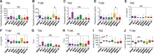
Hormones (testosterone, luteinizing hormone, LH, and inhibin B) quantification by immunological assays. Intra-testicular (A, B) or blood (C, D) testosterone concentrations were determined in male rats at T90 (A, C) and T180 (B, D). Circulating LH was determined in males at T90 (E) and T180 (F) and the ratios of circulating testosterone versus LH (T/LH) level were determined at T90 (G) and T180 (H). Circulating inhibin B in males was determined at T90 (I) and T180 (J). The assay was performed with 10 (subgroup A) or 12 (subgroup B) samples per diet group respectively at T90 and T180. Adjusted p values from Kruskal Wallis test (post hoc Dunn’s adjustment) are indicated (*p < .05). Abbreviation: NS, not significant.
In females, no ovarian abnormalities were noted between the 8 groups (Supplementary Table 8B), suggesting an absence of effect of the diets on ovarian function. The hypothalamo/pituitary/ovary axis was analyzed by quantifying estradiol (E2), LH, and FSH levels in plasma. E2 levels showed no significant difference between the 8 groups at both feeding times (Supplementary Figs. 5A and B). Likewise, there was no difference in circulating LH (Supplementary Figs. 5C and D) and FSH (Supplementary Figs. 5E and F) levels between the groups, confirming the integrity of ovarian function in all of them.
The urinary steroidome was then investigated in each sex: among the 33 targeted steroid hormones, 19 were detected with significant consistency (ie, detection rate > 50%) in females, whereas only 6 and 8 were significantly detected in males at T90 and T180. In male samples collected at T90, the difference between the diet groups was significant only for pregnenolone and progesterone among the 6 hormones considered (Table 7
Analysis of 19 Urinary Steroid Hormones (Steroidome) by Mass Spectrometry
| Steroid Hormone | Males T90 | Females T90 | Males T180 | Females T180 |
|---|---|---|---|---|
| Pregnenolone | <0.001 | 0.223 | 0.436 | 0.078 |
| 17αOH-pregnenolone | nd | 0.777 | nd | 0.307 |
| DHEA | nd | 0.628 | nd | 0.024 |
| 5-Androstene-3β, 17β-diol | nd | 0.315 | nd | 0.02 |
| Progesterone | 0.003 | 0.045 | 0.833 | 0.176 |
| 17αOH-progesterone | nd | 0.093 | nd | 0.041 |
| Androstenedione | 0.536 | 0.084 | 0.845 | 0.338 |
| 17β-Testosterone | 0.481 | 0.081 | 0.262 | 0.22 |
| 5α-Pregnane-17α-ol-3, 20-dione_(17αOH-dihydroprogesterone) | nd | 0.548 | nd | 0.231 |
| 5α-Androstanedione | 0.439 | 0.809 | 0.04 | 0.163 |
| 5α-Dihydrotestosterone_(5α-DHT) | nd | 0.02 | nd | 0.129 |
| 5α-Pregnane-3α-ol-20-one_(allopregnanolone) | nd | 0.254 | nd | 0.276 |
| 5α-Pregnane-3α, 17-diol-20-one_(17αOH-allopregnanolone) | nd | 0.534 | nd | 0.463 |
| Androsterone | 0.055 | 0.213 | 0.127 | 0.258 |
| Epiandrosterone | nd | 0.85 | 0.169 | 0.673 |
| 5α-Androstane-3β, 17α-diol | nd | 0.414 | nd | 0.034 |
| 5α-Androstane-3β, 17β-diol | nd | 0.681 | nd | 0.783 |
| 17β-Estradiol | nd | 0.112 | nd | 0.379 |
| Estrone | nd | 0.052 | nd | 0.235 |
The table reports the results of the comparison between the different groups of rats (males, females, T90 and T180) fed with the considered formulations in terms of urinary steroid hormone levels, for each gender and each sampling collection time (nonparametric KW test). Significant p values (p < .05).
Abbreviation: nd, non-determined due to non-detected/<LOD values or detection rate <50%.
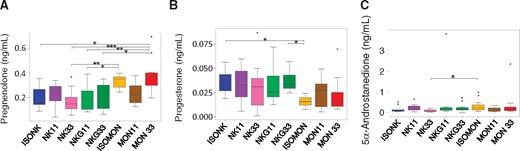
Box-plots presenting urinary concentrations of hormone steroids (pregnenolone, progesterone, and 5α-androstanedione) in male rats (subgroup B). Determination of pregnenolone (A) and progesterone (B) concentrations at T90 (12 samples per diet group). Determination of 5α-androstanedione (C) concentrations at T180 (11–12 samples per diet group). Adjusted p values from Mann-Whitney tests (post hoc Tukey adjustment) are indicated (***p ≤ .001; **0.001 < p ≤ .01; *0.01 < p ≤ .05).
In female samples collected at T90, a significant difference was observed for 2 of the 19 hormones investigated, namely pregnenolone and 5α-dihydrotestosterone (Table 7). However, the difference remained significant only for 5α-DHT after an adjusted Mann-Whitney test (Figs. 3 A and B). The tendency previously observed for pregnenolone in males was not observed. For samples collected at T180, there was a significant difference for 4 of the 19 hormones, namely DHEA, 5-androstene-3β, 17β-diol, 17αOH-progesterone and 5α-androstane-3β, 17α-diol (Table 7). After post hoc adjustment, this statistical difference remained only for DHEA between groups fed ISONK and NK11 diets, and for 17αOH-progesterone between groups ISOMON and ISONK as well as between groups fed ISOMON and NK-G33 diets (Figs. 3C–F).
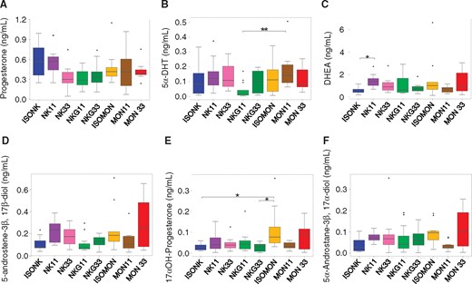
Box-plots presenting urinary concentrations of hormone steroids (progesterone, 5α-DHT, DHEA, 5-androstene-3β, 17β-diol, 17αOH-progesterone and 5α-androstane-3β, 17α-diol) in female rats (subgroup B). Determination of progesterone (A) and 5α-dihydrotestosterone (B) at T90. Determination of DHEA (C), 5-androstene-3β, 17β-diol (D), 17α-hydroxyprogesterone (E), and 5α-androstane-3β, 17α-diol dehydroepiandrosterone (F) at T180. The measurement was performed with 10–12 samples per diet group. Adjusted p values from Mann-Whitney tests (post hoc Tukey adjustment) are indicated (***p ≤ .001; **0.001 < p ≤ .01; *0.01 < p ≤ .05).
Altogether, we observed very few differences in terms of the urinary endogenous steroid profile. In addition, these differences are not biologically consistent with regard to the steroidogenesis pathways, their interpretation in physiological terms was impossible despite their statistical significance. In summary, our steroidomic data did not show any significant disruption of the steroidome for males and females exposed to a GM-based diet after a 90- or 180-day feeding period.
Liver and Kidney Transcriptome
To obtain deeper insight into a putative effect of GM feed in rat physiology, a full transcriptomic (liver and kidney samples) and metabolomic (plasma and urine samples) analysis was conducted. We first performed PCAs with the liver transcriptome of rats sacrificed 180 days (T180) after the beginning of the GMO-protocol. We observed as expected a clear separation between 2 groups of individuals perfectly identified by the sex factor (Figure 4 A). This result is also found with the kidney transcriptome (data not shown). On the contrary, a very low variability due to any other factors such as diet was observed with the results of the liver transcriptome at T180 (PC3 and PC4: 2% of explained variability; Figure 4B). A similar pattern of variability was observed with the data from the liver transcriptome of subgroup A (T90) as with the kidney transcriptome at different time points (data not shown). Overall, this first descriptive exploratory analysis suggested no clustering effect of the different diets; the sex factor was responsible for a high variability in the transcriptomic profiles analyzed. First a global PLS-DA was performed per each sex. In male rats, the results obtained from liver samples at T180 showed a very low variability according to the diets and no clear distinction was observed between them (Figs. 5 A–D). Results were similar at T90 for liver and at both experimental times for kidney, and overall for the females (data not shown). The next step was to examine a selection of diets for an effect of glyphosate treatment, maize variety in the diet, and GM- versus non-GM diet. Because glyphosate levels were similar in all the diets, our experimental plan allowed us only to test the indirect effect of the glyphosate treatment of NK603, ie, the effect of metabolic changes in kernel composition induced in the growing plants (hereafter termed “glyphosate effect”). In liver at T90, the number of differentially expressed genes (DEGs) was 1 when NK33 versus NKG33 conditions were compared in females (Table 8
Number of Statistically Differentially Expressed Genes (mRNA) or miRNA Between Each Relevant Diet Condition (Based on Pairwise Comparison Between Diets) in the Rat Liver or Kidney Samples at T90 and T180
| Liver | Kidney | ||||||||||||||||
|---|---|---|---|---|---|---|---|---|---|---|---|---|---|---|---|---|---|
| mRNA | miRNA | mRNA | miRNA | ||||||||||||||
| Female | Male | Female | Male | Female | Male | Female | Male | ||||||||||
| T90 | T180 | T90 | T180 | T90 | T180 | T90 | T180 | T90 | T180 | T90 | T180 | T90 | T180 | T90 | T180 | ||
| Glyphosate effect | NK11 vs NKG11 | 0 | 0 | 0 | 0 | 0 | 0 | 0 | 0 | 0 | 0 | 0 | 3658 | 0 | 0 | 0 | 0 |
| NK33 vs NKG33 | 1 | 0 | 0 | 0 | 0 | 0 | 0 | 0 | 0 | 0 | 0 | 0 | 0 | 0 | 0 | 0 | |
| Variety and environment effect | ISOMON vs ISONK | 5 | 4 | 5 | 16 | 0 | 0 | 0 | 0 | 0 | 1 | 1 | 6 | 0 | 0 | 0 | 0 |
| MON11 vs NK11 | 4 | 8 | 90 | 284 | 0 | 0 | 0 | 0 | 0 | 1 | 3 | 795 | 0 | 0 | 0 | 0 | |
| MON33 vs NK33 | 3 | 5 | 4 | 7 | 0 | 0 | 0 | 0 | 1 | 0 | 6 | 4 | 0 | 0 | 0 | 0 | |
| GM effect | MON11 vs ISOMON | 0 | 2 | 0 | 0 | 0 | 0 | 0 | 0 | 0 | 0 | 0 | 0 | 0 | 0 | 0 | 0 |
| MON33 vs ISOMON | 1 | 0 | 0 | 0 | 0 | 0 | 0 | 0 | 0 | 0 | 0 | 822 | 0 | 0 | 0 | 3 | |
| MON33 vs MON11 | 0 | 0 | 0 | 0 | 0 | 0 | 0 | 0 | 0 | 0 | 0 | 563 | 0 | 0 | 0 | 0 | |
| NK11 vs ISONK | 0 | 0 | 0 | 11 | 0 | 0 | 0 | 0 | 1 | 0 | 0 | 0 | 0 | 0 | 0 | 0 | |
| NK33 vs ISONK | 0 | 0 | 0 | 0 | 0 | 0 | 0 | 0 | 1 | 0 | 2 | 1 | 0 | 0 | 0 | 0 | |
| NK33 vs NK11 | 0 | 0 | 0 | 0 | 0 | 0 | 0 | 0 | 0 | 0 | 0 | 0 | 0 | 0 | 0 | 1 | |
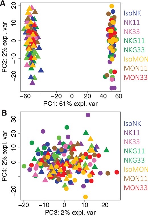
Principal component analysis using data generated with liver mRNA of rats sacrificed at T180. Each diet is identified by a specific color and correspondence is shown in Table 2. Each female is identified with a triangle whereas each male is identified with a circle. A, The first 2 principal components explaining variability are represented on x-axis (PC1) and y-axis (PC2). A clear separation between males (circles) and females (triangles) is observed (PC1: 61% explained variability). B, The second and third principal components explaining variability are represented on x-axis (PC3) and y-axis (PC4). No clustering effect of the different diets is observed.
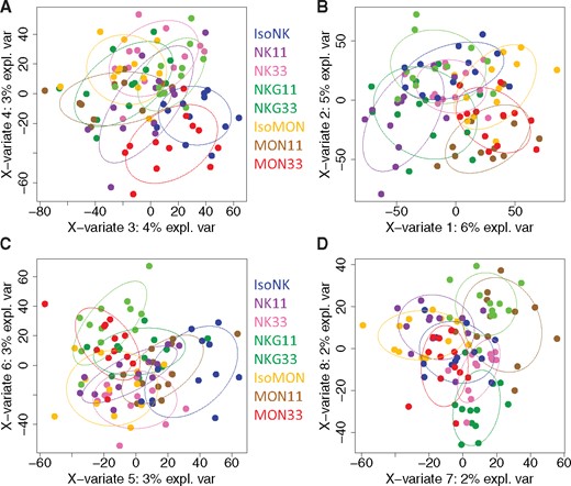
Partial least squares-discriminant analysis between the 8 diets based on liver transcriptome variables from males (circles) at T180; variability is represented on the x-axis (PC1) and the y-axis (PC2) (A), x-axis (PC3) and y-axis (PC4) (B), x-axis (PC4) and y-axis (PC5) (C), x-axis (PC6) and y-axis (PC7) (D). No clear clustering was observed between the 8 diets.
The genetic background of maize (MON or NK) in conjunction with the growing area (Spain for MON or Canada for NK) may lead to different omics signatures. sPLS-DA, which sharpens the separation between groups of observations using the twenty most discriminative variables, shows a clear distinction between both MON810 and NK603 diets (Figure 6 ). Interestingly, liver transcriptomic analysis revealed the highest number of DEGs when comparing MON versus NK diets. At T90, various genes were differentially expressed significantly in the liver of both sexes in the 3 conditions ISOMON versus ISONK, MON11 versus NK11, and MON33 versus NK33 (Supplementary Tables 11 and 12). The number of DEGs was far below the total number of DEGs linked to the sex effect and no biological relevance could be established owing to the lack of information related to these changes or to the lack of difference in biologically linked variables for all comparisons. No DEMI was significant (Table 8). When analyzing kidney-related transcriptomics data at T90, we found a lower number of DEGs 0, 0, and 1 in females and 1, 3, and 6 in males (Table 8, Supplementary Table 13). At T180, we found a low number of DEGs in females but not in males (Supplementary Table 14). No DEMI was significant (Table 8).
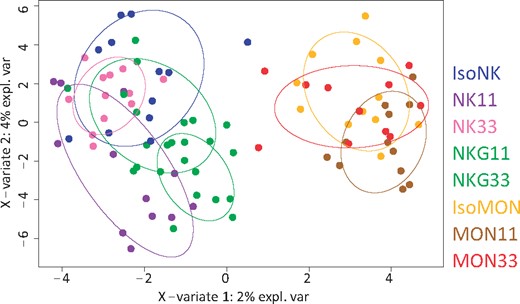
sPLS-DA (sparse Partial least squares-Discriminant Analysis) between the eight diets based on liver transcriptome variables from males at T180. The twenty most discriminative variables were selected on each component by the sparse model. The samples are projected to the components 1 and 2. A clustering is observed on the x-axis with a clear separation between both NK603 (left) and MON810 (right) diets.
The main objective was to evaluate the effect of GMO versus non-GMO consumption. In female livers, the number of DEGs was only 1 at T90 in MON33 versus ISOMON conditions and 2 at T180 in MON11 versus ISOMON conditions whereas in male livers, the number of DEGs was 11 at T180 in NK11 versus ISONK conditions (Supplementary Table 15). No other modifications (DEGs, DEMI) were observed in male or female livers. In kidney, the number of DEGs was very low (1) at T90 when comparing NK11 versus ISONK and NK33 versus ISONK in females. In male kidneys, the number of DEGs was quite high (822 and 563) at T180 in MON33 versus ISOMON and MON33 versus MON11 conditions, but remarkably low (2 and 1) when comparing NK33 versus ISONK conditions at T90 and T180 (Table 8, Supplementary Table 16). The number of DEMI was low (3 and 1) in MON33 versus ISOMON and NK33 versus NK11 conditions in males (Supplementary Table 16).
Urine and Plasma Metabolomic
The results from the PCAs with the data generated by urine or blood metabolome was similar to that observed with liver and kidney transcriptome showing a clear sex effect (data not shown). A PLS-DA on metabolomic data was performed per each sex (Figure 7 ). The results showed a very low variability according to the diets and no clear distinction was observed between them (data not shown).
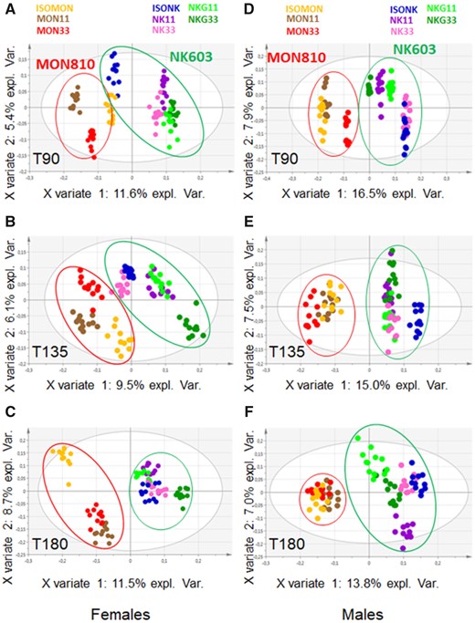
Partial least squares-discriminant analysis between 8 diets based on urine metabolome variables at T90 (A, D), T135 (B, E), and T180 (C, F); (A–C) females and (D–F) male rats. A clustering is observed on the x-axis with a clear separation between both MON810 (left) and NK603 (right) diets.
Then, the indirect glyphosate effect was tested using the plasma or urine metabolomics data at T90, T135, and T180 (Table 9
Number of Statistically Differential Metabolites Between Each Relevant Diet Condition (Based on Pairwise Comparison Between Diets) in Rat Plasma or Urine Metabolomic Profiles at T90, T135, and T180
| Plasma | Urine | |||||||||||||
|---|---|---|---|---|---|---|---|---|---|---|---|---|---|---|
| Female | Male | Female | Male | |||||||||||
| T90 | T135 | T180 | T90 | T135 | T180 | T90 | T135 | T180 | T90 | T135 | T180 | |||
| Glyphosate effect | NK11 vs NKG11 | 0 | 0 | 0 | 0 | 0 | 0 | 2 | 1 | 3 | 3 | 0 | 4 | |
| NK33 vs NKG33 | 0 | 0 | 0 | 0 | 0 | 0 | 2 | 5 | 4 | 4 | 5 | 1 | ||
| Variety and environment effect | ISOMON vs ISONK | 0 | 1 | 0 | 1 | 3 | 7 | 0 | 3 | 3 | 3 | 4 | 11 | |
| MON11 vs NK11 | 0 | 7 | 2 | 3 | 0 | 6 | 20 | 17 | 17 | 11 | 2 | 11 | ||
| MON33 vs NK33 | 0 | 4 | 1 | 4 | 0 | 2 | 13 | 7 | 8 | 6 | 5 | 11 | ||
| GM effect | MON11 vs ISOMON | 0 | 0 | 0 | 0 | 0 | 0 | 9 | 2 | 13 | 2 | 2 | 0 | |
| MON33 vs ISOMON | 0 | 0 | 0 | 0 | 0 | 0 | 1 | 3 | 8 | 0 | 1 | 3 | ||
| MON33 vs MON11 | 0 | 0 | 0 | 0 | 0 | 0 | 7 | 4 | 3 | 3 | 4 | 2 | ||
| NK11 vs ISONK | 0 | 0 | 0 | 0 | 0 | 0 | 14 | 8 | 3 | 6 | 1 | 4 | ||
| NK33 vs ISONK | 0 | 0 | 0 | 0 | 0 | 0 | 8 | 2 | 4 | 0 | 1 | 1 | ||
| NK33 vs NK11 | 0 | 0 | 0 | 0 | 0 | 0 | 1 | 4 | 2 | 4 | 1 | 2 | ||
Similarly to the transcriptomic analysis, we observed a maize variety and environment effect. For plasma, a blinded analysis performed per sex showed a clear effect because the concentrations of 9 and 13 metabolites were significantly altered in males and females, respectively, which had consumed the ISOMON, MON11, or MON33 diet in comparison with the other diets. Then, unblinded data allowed discriminating the MON and NK diets on the basis of 8, 3 and 15 metabolites in males and 0, 1 and 3 metabolites in females, at T90, T135, and T180, respectively (Table 9). The diets could be discriminated by a few plasma metabolites repeatedly found at slightly different concentrations: stachydrine, methionine sulfoxide, 2-ceto-4-methylthiobutyric acid (KMBA), and 1,5-anhydro-d-sorbitol in males (0.97 < ratios < 1.03) and stachydrine, ergothioneine, eugenol, and 2-furoic acid in females (0.97 < ratios < 1.03) (Supplementary Table 20). For urine, a clear discrimination was also found between the 3 diet pairs. For example, the comparison between ISOMON versus ISONK, except at T90 in females, provided a model with a high level of prediction (2 elements, R2 close to 100%, Q2 close to 1). Similar results were obtained for both sexes at all timepoints when comparing MON11 versus NK11 and MON33 versus NK33. PLS-DA showed that at T90, T135, and T180 and in both sexes except females at T90, the concentrations of 2–20 metabolites in urine were significantly altered (Table 9, Supplementary Tables 17–19). The difference in metabolite levels was more pronounced with NK11 versus MON11 and NK33 versus MON33 than with ISONK versus ISOMON, as was the case for the female urine compared with the male urine. Considering the same prerequisites as above, the significantly altered metabolites evidenced by comparing NK versus MON diets are shown in Supplementary Tables 17–19. However, only the concentrations of cis-aconitic acid, pantothenic acid, and trigonelline were modified more than once when comparing the 3 diets at the 3 timepoints for males and 2-oxoglutaric acid for both males and females. In conclusion, omics data indicated that the MON diets were clearly different from the NK ones, the best separation being obtained with metabolites quantified in urine.
We then studied the GM-effect with MON- and NK-based diets. For plasma, no modification was identified (Table 9). For urine, the model was valid for both females and males, except at T180. The MON GM versus non-GM diets could be discriminated (4 or 5 elements, R2 close to 95%, Q2 close to 0.8) but the models were less predictive than those testing the effect of maize genetic background. PLS-DA obtained at T90, 135, and 180 showed few alterations in the metabolites (Table 9, Supplementary Tables 17–19). Using the same prerequisite as aforementioned, only the concentrations of glucuronic acid and indoxylsulfate were found to be altered in urine when the pairs of MON diets were compared in females, whereas only citric acid was modified in males. In the case of NK-based diets, the models were not valid for females at T135 and T180 or for males at T90. The differentiation between the NK GM versus non-GM diets was obtained with a low level of prediction (Q2 about 0.6). PLS-DAs indicated several modifications that had occurred in both males and females at the 3 timepoints (except for 1 out of 18 comparisons) and with all the diets. The modifications were more pronounced in females than in males. However, using the prerequisite aforementioned, only dimethylamine and glycocholic acid were altered in females and 2-oxoglutaric acid in males. The differential concentrations of these metabolites in urine could not be correlated with any pathophysiological signature.
DISCUSSION
The GMO90+ sub-chronic feeding trial was designed to fulfill multiple goals by combining a classical toxicology study following the OECD TG 408 guidelines (with modifications) and omics approach. To our knowledge, this is the first time that MON810 and NK603 maize-based diets were used side by side to feed rats for 6 months to analyze potential GMP effects on the basis of a large number of parameters including pathologic to molecular markers. In line with transparency in research activity on the health impact of GMP, a dialog body has tentatively been set up to promote public participation as a way to increase trust in institutional practices. The causes of the failure of operating this instance are currently being analyzed and the conclusions will be reported elsewhere. The quality and equivalence of the different diets was ensured by a complete compositional analysis in which a large number of molecules were detected and quantified by targeted analyses (Chereau et al., 2018). The nutrient and antinutrient composition of the diets showed no substantial differences as with contaminants between GM and non-GM or NK and NKG pellets. The data for glyphosate were surprising. Indeed, all diets were found to contain glyphosate, with slightly higher levels in NKG-based pellets, whereas glyphosate had only been detected in NKG grains. It is likely whereas unexpected that the presence of glyphosate residues in all diets results from a weak contamination of the organic soybeans culture from South America. Consequently, a “glyphosate effect” can only be tested as an indirect effect on maize composition not on rat health. This was referred to as the “glyphosate effect” throughout this study. However, 2 differences were observed with fumonisins and lead contaminants present at higher level although at nontoxic dose, in MON- by comparison with NK-based diets. In addition to classical targeted biochemical analyses, we also performed metabolomic analyses of the pellets (Bernillon et al., 2018). Again, the great majority of statistically significant differences in composition of the pellets, was attributed to the combined effect of variety and environment. In comparison, transgene and glyphosate effects remained limited in grain and pellet for the compound families studied.
The rat body weight was measured for 3 months (subgroup A) and 6 months (subgroups B and C) feeding trial. There was no significant difference between the diet groups for either feed consumption or body weight of rats of both sexes and consequently no GM effect with both MON- and NK-based diets. A limited number of minor clinical signs were observed mostly in rats of both sexes from subgroup B which manifested about 66% of clinical signs, whereas subgroups A and C manifested about 33%. This might have been due to a higher level of stress in this subgroup which underwent blood tests on the jugular vein (times T0, T90, and T135) and urine collection in metabolic cages for 5 days (T90, T135, and T180). No difference between GM versus non-GM diets was observed. Similarly, gross necropsy findings did not provide evidence for a biologically relevant difference between GM versus non-GM feed, nor did macroscopic and evaluation of the organs and tissues in both males and females. Microscopic histopathologic analysis identified few abnormalities in animals fed the different diets, but a lack of evidence for a GM-diet effect. All these results are in accordance to that reported previously by the GRACE EU-funded project (Zeljenková et al., 2014, 2016).
The main objective of the project was to identify biological and omics markers of exposure and potentially of effects to discriminate a GM-based diet in comparison with a near isogenic non-GM diet. The difference between GM versus non-GM diets on hematologic parameters in males only concerned the mean thrombocyte volume within the NK-G33 diet group, but not the other groups, and at T90 but not at T180. Similarly, the difference in hematologic parameters in females concerned the albumin/globulin ratio and eosinophils (%) in one diet group (**NK11 and NK-G11 respectively) and at one feeding time (T90 and T180, respectively). The difference between GM versus non-GM diets on clinical biochemistry parameters concerned triglycerides only in males in the NK-G11 diet group and at T180. Kidney function is very often impaired earlier than other functions in animals exposed to a wide variety of toxic agents and was previously reported altered in rats fed with GM corn varieties by comparison with non-GM diet (de Vendômois et al., 2009; Séralini et al., 2014). Consequently, we monitored urine parameters to assess kidney functions in addition to necropsy and microscopic observations. No statistical difference was found in the effect of GM- and non-GM diets. Despite few significant differences in biological parameters between the diet groups, most of them correspond to a maize variety and environment effect and not to a GM maize effect. We do not consider that these differences are biologically significant because none of them showed a dose/response effect and numerous similar differences existed in other pairwise comparisons. Our results are in accordance with the large majority of the reports (Bartholomaeus et al., 2013; Snell et al., 2012) as well as with the GRACE EU-funded project (Schmidt et al., 2017; Zeljenková et al., 2014, 2016).
The investigations on reproductive function in males and females evidenced only marginal effects in the male groups and none in the female groups as already reported for BT799, a maize expressing the Cry1Ac gene (Guo et al., 2015). Hormonal profiles in males and females were established by immunological quantification in plasma and by the characterization of potential disruptions induced by the diets at the steroidogenesis level analyzed by MS measurements of urine samples. We observed a difference in male urine samples collected after 90-day feeding only for pregnenolone and progesterone (Table 7). However, differences were observed between the MON and NK-fed groups but not between MON or NK and their corresponding non-GM controls. In addition, these differences were observed at T90 but not T180. The biotransformation of pregnenolone into progesterone is mainly mediated by 3β-hydroxy-δ5-steroid dehydrogenase (HSD3B) and the steroid δ-isomerase. The eventual inhibitory effect of the diets on these enzymes would require additional investigation. In the case of a potential effect, the inhibition mechanism will not rely on transcriptional regulation because no variation of the corresponding mRNAs was found (Supplementary Table 11).
The differences observed are not biologically relevant in light of the different GM percentages in the diets, the sex, the experimental time, the links between the biological variables, the clinical signs, and the microscopic evaluation of the tissues. Most differences in biological parameters were linked to the variety or environment effect in accordance with contaminants differentially recovered in the MON- versus NK-based diets. Then, the integration of data at T180 from 5 datasets (kidney parameters, hormonal dosage, urine steroidome, biochemical data, and organ weights) was conducted per each sex. Despite the focus on diet discrimination, we could not obtain convincing results to differentiate the diets.
The highly sensitive multiomics approach was planned to decipher the complex physiological response pattern of rats when exposed to diets despite the lack of substantial differences in nutrient, antinutrients, and contaminants between GM and non-GM as well as between NK and NKG diets. Both mRNA and miRNA expression in liver and kidney differed between males and females. However, the global analysis based on pairwise analyses of the diets showed a lack of variation in miRNA between males and females. Some variations in mRNA expression between the groups fed different diets were observed but no signature could be assigned to distinguish the groups (Figs. 4 and 5). The pattern of DEGs between the groups and biochemical or pathological parameters could not be assigned, as previously reported for rats fed with NK603 ± glyphosate (Mesnage et al., 2017). In fact, the pattern of mRNA expression between samples is currently used to characterize sets of genes involved in specific metabolic pathways but not as a tool to differentiate samples. In contrast, the metabolomic data discriminated the diets better when urine was tested, rather than plasma. Possible explanations are that urine as the final metabolic compartment of an organism cumulates effects, that metabolites are differentially present in the 2 sample biofluids or that LC-HRMS (plasma) detects other types of metabolites than 1H NMR (urine). Indeed, because the composition of each diet was different, urine analysis could be expected to discriminate the diets. Variations in metabolite concentrations were analyzed to investigate a potential dietary effect linked to GM food, glyphosate treatment, or maize variety.
An effect of the GM-based diet was tested with both the MON and NK harvests. In contrast to the effect observed by globally comparing the varieties (transcriptome and metabolome), only the data from the urine metabolome allowed the diets to be differentiated. It is noteworthy that the chemical analysis of urine also differentiated the 8 types of pellets. The few significant differences observed could be due to exposure to GM-based diets versus ISOMON or ISONK controls, but not to a potential health effect. In fact, the search for an effect of GM-based food on various health parameters such as kidney, liver, and reproductive physiology was not fruitful, in accordance with the findings of the GRACE project (Zeljenková et al., 2014, 2016).
An effect of the treatment with glyphosate was tested although similar herbicide residue concentrations (no significant difference) between diets were quantified. This did not allow us to evidence any direct effect of glyphosate on rat health. In addition, owing to the low level of contamination of the diets, glyphosate could not be quantified in kidney or liver extracts as previously reported (Mesnage et al., 2017). A few metabolites in urine, but not in plasma, allowed the NKG- and NK-based diets to be differentiated. A slight decrease in taurine was found in females with the NKG diets, with a dose effect apparent between the NKG33 and NKG11 diets at T135 and T180. No such modification was found in males, but there was a slight increase in indoxylsulfate at T90 and T135. Indoxylsulfate is a uremic toxin that is produced in the liver from indole, a tryptophan derivative, of which increased levels are associated with chronic kidney disease (<3 µM in normal conditions in humans vs > 20 µm in uremia patients). However, neither histopathological nor pathophysiologic examinations of kidneys indicated any damage. The slight variations in urine metabolites cannot be associated with any biological disturbance, are not indicative of any health effect and argue against an indirect effect of glyphosate. Other authors using transcriptomic and metabolomic analyses of kidney and liver samples reached a similar conclusion (Mesnage et al., 2017). Moreover, a recent transcriptomic analysis of gut tissues of rats fed with MON810 and the near-isogenic control did not reveal any significant GM-related changes in expression profiles (Sharbati et al., 2017).
On the contrary, we could discriminate the groups fed with MON or NK varieties; this is in line with the significant differences in the composition of the corresponding pellets attributed to the combined effect of genotype and environment (Bernillon et al., 2018). More specifically, the analysis of the liver transcriptome in males allowed us partly to discriminate the 2 varieties (Figure 6); a similar result was obtained with the kidney transcriptome in males and females. Interestingly, common genes were expressed differently in both male livers and kidneys over time (T90 vs T180), such as Spw1 (selenoprotein W) and Gpx1 (glutathione peroxidase 1), which are both involved in oxidation-reduction reactions. Because fumonisins B1 and 2 alter the cellular redox balance (Rumora et al., 2007; Wang et al., 2016), the increased expression of messengers coding for redox-sensitive signaling molecules (and potentially transcriptionally regulated by redox-sensitive transcription factors) might be due to the contamination of MON-based diets in comparison with NK-based diets (Chereau et al., 2018). Fumonisins are mycotoxins produced by toxigenic Fusarium species characterized by a structural similarity to sphinganine and which consequently are able to strongly inhibit the ceramide synthase (Edite Bezerra da Rocha et al., 2014). Despite a high number of DEGs at T180 in the kidney, no major signaling pathway was significantly identified in the whole sample. Metabolomic data on the grains showed that MON harvests had a higher content in betaine, proline, valine, alanine, GABA, and succinic acid, whereas NK harvests had higher contents in several sugars or sugar alcohols, malic acid, fumaric acid, aspartic acid, glutamic acid, choline, tyrosine, and tryptophan (Bernillon et al., 2018). No clear correspondence between the metabolic data of the diets and plasma samples could be established. Several hypotheses could explain this finding: the composition of the pellets (only 33% of maize), thereby minimizing differences between the maize harvests, the major role of the microbiota in the production of absorbed metabolites and slight differences in the nutritional composition of MON- and NK-based diets. In comparison, a clearer separation between the groups was observed using the metabolomics data obtained from urine. Based on PLS-DAs, the 2 varieties could be differentiated for both sexes, as shown in Figure 7. No link between maize kernel composition and the metabolic signature of exposure in urine could be established. In addition to variations in nutritional content, the 2 varieties were different in the nature and extent of their contaminants; as indicated above, a major difference was the 10-fold lower contamination of NK-based kernels by fumonisins than in MON kernels (Chereau et al., 2018). The increased ratio of sphinganine/sphingosine in urine has been proposed as a biomarker of fumonisin exposure in humans (Solfrizzo et al., 2004). However, the 1H NMR determination used in our study did not allow these metabolites to be quantified in urine.
In conclusion, we identified no early biomarker of exposure or effect that could be added to the conventional 90-day rodent study required in the framework of the European regulation 503/2013 and the multiomics experiments did not bring new findings on a potential effect of GM-based diet. The results are in agreement with previous reports claiming the limited effect of GM feed in comparison with non-GM near-isogenic feed.
At last, we showed in accordance with the results from GRACE and G-TwYST projects that the added scientific value of subchronic 90-day studies animal feeding studies, without a targeted hypothesis might be limited and not significantly reduce remaining uncertainties (Bartholomaeus et al., 2013; Kuiper et al., 2013). In the long term, 90-day or extended animal feeding studies might still be justified when there is a particular concern identified during the risk assessment procedures.
SUPPLEMENTARY DATA
Supplementary data are available at Toxicological Sciences online.
ACKNOWLEDGMENTS
We thank Drs Pablo Steinberg, Ralf Wilhelm, and Joachim Schiemann (G-TwYST, EC project) for sharing their maize production and preliminary targeted analyses of the grain, and Dr Maria Pla (IRTA Mas Badia Field Station) for providing the grain samples cultivated in Spain. We are grateful to the members of the scientific council of RiskOGM program for their follow-up and advice. B.J. is Prof. at EHESP—School of Public Health, Rennes (France). The authors declare no conflicts of interests. Public declaration of interests is available on the public RiskOGM programme website (http://rechercheriskogm.fr/en/page/partners-pdis).
FUNDING
The funding was from the Risk'OGM research program of the french Ministry for an Ecological and Solidary Transition (RiskOGM program).
AUTHORS’ CONTRIBUTIONS
Designed research: XC, RS, BJ, LD, EJ, JPC, NS, FF, FRF, RB, PR, BS
Performed research: LJ, YKA, LB, CN, MLM, CDL, CC, JC, SB
Analyzed data: XC, RS, LF, YL, JPA, BJ, MTF, CLG, JL, PAG, KDA, NA, BC, AM, BL, BS
Wrote the paper: XC, BS
COMPLIANCE WITH ETHICAL STANDARDS
The rodent experimentation conducted at CitoxLAB CRO was approved by the French Ethical Committee (CETEA) No. 3148—July 21, 2015.
REFERENCES
Tillé, Y., and Matei, A. (2016). sampling: Survey Sampling. R package version 2.8. https://CRAN.R-project.org/package=sampling.
Author notes
These authors contributed equally to this study.

Comments