1. Introduction

During most of the twentieth century, the photogrammetry required a lot of monetary and time resources. After the technological development of electronic systems like the Global Positioning System (GPS) and the Inertial Measurement Unit (IMU), the design of autonomous vehicles, and the production of digital cameras, time and cost limitations have been steadily declining. Thus, the rise of the Unmanned Aerial Vehicles (UAVs) started. Nowadays, there is a wide range of UAVs with multiple sensors and digital cameras that are being used in many different areas such as photogrammetry, agriculture, management of natural resources, mapping and urban planning, rescue [1], assessment and mitigation of disasters, and other Remote Sensing applications [2].

One of the most important and common uses given to the aerial images acquired by UAVs, also known as drones, is the image mosaicking, which allows better visualization and assessment of an event or area of study. For instance, the usage of image mosaicking in agriculture [3] is beneficial not just because it generates an image that covers bigger areas of crops with high resolution, in fact, it also allows control the temporal resolution and the periodical assessment of the fields to improve decision-making regarding the amounts of pesticides, irrigation, land usage, and other variables.

Image mosaicking is about the reconstruction of a scene in two dimensions (2D) by using individual images with overlapping areas. In order to perform this process, the estimation of geometric transformations between pairs of images is required to project them over the others and merge them together with the minimum possible error. These projective transformations, which are commonly known as 2D homographies, are estimated from matching points of two overlapping images.

Multiple mosaicking algorithms have been developed depending on the requirements of accuracy and time. There are high accuracy algorithms based on Structure from Motion technique that estimates the scene information in three dimensions, the orientation and the localization of the camera, and in this way, it calculates the homographies [4]; however, these algorithms imply high computational cost and are difficult to implement. Other algorithms utilize the information of the GPS and gyroscope of the UAV to obtain approximations of localization and orientation of the cameras during the flight [5] but matching images and gyroscope information by the acquisition time may not be accurate. In addition, it has been implemented algorithms that perform feature matching based on bag of words (BoW) and dictionaries [6, 7] to accelerate this step, for example, in [8] author compared processing times of different methods of feature matching. Moreover, other researchers have modified the Structure from Motion technique and have changed the Bundle Adjustment by other techniques of global adjustment [9, 10]; nevertheless, these algorithms are difficult to implement.

We present a simple method of mosaicking aerial images with geographical information acquired by UAV that obtains viable results for applications in natural resources monitoring, and competitive results in terms of processing time and geolocation error, in comparison with professional software. This method is based on the image mosaicking of aerial images acquired in the same line of flight, and the usage of symmetric transfer error per inlier as an indicator of acceptable estimation of the homography.

This work is organized as follow: Section 2 develops the proposed mosaicking algorithm and the implementation details. In section 3, the results are presented and compared with those of one professional software. Finally, in section 4, we present the conclusions and comment some limitations of the proposed algorithm.

2. Proposed Method

The proposed method is based on a modification of the Random Sample Consensus (RANSAC) method used to automatically estimate homographies. According to Figure 1, this method first creates a mosaic of all images acquired in the same line of flight and then obtains the final mosaic by merging properly the mosaics of flight lines. Given that our method is based on the flight trajectory, first, we mention some details related to the acquisition of images via UAV: the images must be composed of three channels (the most common case is RGB), and they should be geotagged (latitude and longitude) in order to obtain flight lines and to perform the georeferencing step. In this section, we describe and explain the implementation details regarding the steps of the proposed method.

2.1        Image Reading and Image Preprocessing

The first step is to read geotagged images and obtain the number, the names, the directory, the size and the geographical information of the images. Then the images are resized to a maximum resolution of 1500 x 1000 pixels and the geographical information is transformed to the Universal Transverse Mercator (UTM) coordinate system.

The preprocessing consists of the selection of images that belong to the same flight lines, which are almost straight lines as those of Figure 2. It is important to understand that the geolocation information of each image corresponds to the point located in the middle of the image. To determine which images belong to the same lines we propose an approach based on the distance between two adjacent images also known as shooting distance.

If the shooting distance between two images is inside a certain range of distances, the method will consider those images have been acquired in the same flight line. The range of distances is established from the most common values of shooting distances and it is calculated as follow:

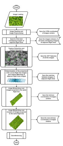Figure 1: Flow Diagram of the proposed mosaicking method.

1. All the shooting distances dist are used to generate a histogram with equally spaced intervals.
2. The most common shooting distance dist_mr is calculated as the mean value of the interval with the larger number of observations or greater frequency.
3. We define the parameter w as the ninth part of the difference between the largest and shortest shooting distance, according to (1). After evaluating the shooting distance for all the geotagged images of different flights, we found that dividing the difference between the boundaries in nine parts performs a better selection of images pertaining to the same flight line.

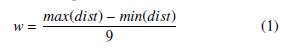4. The range of distances is fixed by (2). The minimum value of this range is the most common shooting distance dist_mr minus two times the parameter w, while the maximum value is the most common shooting distance dist_mr plus five times the parameter w. This is mainly because the majority of shooting distances that do not correspond to images of the same flight line, indicated in the histogram of Figure 3 as red bars, are smaller than dist_mr. The choices of the multiplicative factors 2 and 5 were given after evaluating all the available geotagged images of different flights.

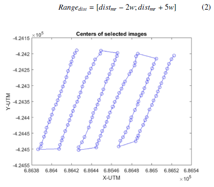Figure 2: Plot of the geolocation of image centers selected for mosaicking.

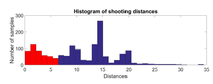Figure 3: Histogram of shooting distances corresponding to six flights.

2.2         Search of the best overlapping images of adjacent flight lines

In order to perform the mosaicking of individual flight lines mosaics, it is required to compute image matching between images of adjacent lines. The optimal procedure is to search for the best overlapping images of adjacent lines rather than perform image matching for all the acquired images due to the time and computational cost. We utilize Delaunay Triangulation [11] and the UTM geographical coordinates of each image to search for pairs of images with enough overlap that belongs to adjacent flight lines. We applied the Delaunay Triangulation algorithm of Matlab that is basically an incremental implementation.

The fundamental property of Delaunay Triangulation can be explain based on the circles circumscribed to a triangle for the 2D case. Given four points V₁, V₂, V₃ and V₄, Delaunay Triangulation is fulfilled when each circle circumscribed to the triangle drawn from three points contains no other point inside of it. The importance of this property is that the majority of the drawn triangles possess relatively large internal angles. Thus, those triangles are considered to be “well shaped” (more similar to an equilateral triangle than to an obtuse one) and for our application, the edges of those triangles connect points that represent two images with enough overlap because the larger edges are smaller than the larger edges of triangles in the non-Delaunay Triangulation.

By applying Delaunay Triangulation, the connections between images with enough overlap are obtained, and shown in Figure 4a; nevertheless, those connections between images of adjacent lines are required to be selected and the rest, to be filtered out. In addition, all the edges of triangles with any internal angle larger than 90 degrees should be deleted to ensure better overlap and therefore more accurate matching points or inliers. After this process, the connections between the images are depicted in Figure 4b.

2.3        Feature Extraction and Feature Description

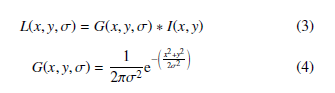
There are many feature extraction techniques in the literature but one of the best techniques used for mosaicking are the Scale Invariant Feature Transformation (SIFT) [12] because of the property to find corresponding points in different scale, rotated and translated images. Images in different scales are the result of convolution between an image I(x,y) and 2D Gaussian filters G(x,y,σ) with different values of standard deviations σ. Equation (3) describes how images in different scales L(x,y,σ) are produced, while (4) describes the 2D Gaussian filter.

SIFT features are located in the local maximum in a neighborhood of 3x3x3 (X-axis, Y-axis and the scale) over the result of the convolution between an image and the difference of the Gaussians with scales k and kσ, as expressed in (5). In addition, the gradients and its orientations are calculated in the neighborhood of the feature.

The first step is feature extraction, also known as feature detection. It computes the detection vector, which is composed of the location in the X-axis and Y-axis, the scale (represented by the standard deviation σ) and the resultant orientation of the gradients. Then, feature description computes the description vector, a 128vector, from the gradients calculated in the neighborhood of the feature point.

Both feature extraction and description are computed by using the implementation of the SIFT algorithm in the open source library VLFeat [13]. Figure 5 shows some SIFT features computed over an aerial image acquired by an UAV over a swampy forest of the Peruvian Jungle in Iquitos, known as Aguajales [14-16].

2.4         Determination of the projection order of one set of flight line images and Feature Matching of sets of adjacent flight lines images

Performing image mosaicking over one set of flight line images requires certain implementation considerations because it implies the projection of images by the homographies, which estimation is not error free. Because of this, determining the projection order is a fundamental step that avoids generating mosaics with visual errors accumulated in certain direction of the image, as the one shown in Figure 6a.

The idea is to project all images over a projection plane aligned with the image located in the middle of the flight line. Therefore, the first image in the projection order is the image in the middle of the line. The next images in the projection order are those that are adjacent to the first one, and then it continues in the same manner but alternating between the two directions of the flight line. This criterion is depicted in Figure 6b.

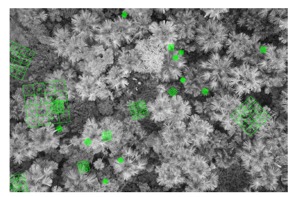Figure 5: SIFT features computation over an aerial image acquired in a forest.

In this step of the proposed method, the feature matching is also performed, between images of adjacent flight lines that were selected in second step of this method. This operation finds two features, one per image, that possess similar SIFT descriptor vectors. We used the SIFT feature matching algorithm implemented in

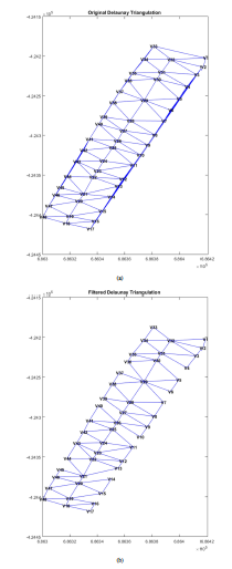Figure 4: Delaunay Triangulation used to search the best overlapping images of VLFeat and we obtained two results: the matches (pair of features) adjacent flight lines (a) Original Triangulation (b) Filtered Triangulation. and the Euclidean distances between them.

The matches between two images are represented as a group of points X_c and X_c⁰; each match is represented as the homogeneous vectors x_c and x_c⁰. These homogeneous vectors are 3-vectors composed by the position of the feature in the X-axis and the Y-axis, and the unity. It is important to mention that the X-axis of the image refers to the horizontal axis (columns) and the Y-axis refers to the vertical axis (rows).

To find the best matches between images of adjacent flight lines, we select the 50 matches with the lowest Euclidean distance for every pair of image established in the second step of the proposed method. By doing this, more than 500 matches can be computed, between images corresponding to two adjacent flight lines that will be used to perform the calculation of homographies between mosaics of flight lines. Any transformation that will be applied to an image during the generation of mosaics of flight lines should be also applied to the features of each image corresponding to the matches between images of adjacent lines because they represent positions over images that are being modified.

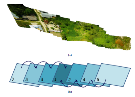Figure 6: Projection order of images: (a) Mosaic generated after projecting the images respect to an image in the end or beginning of line (b) Projection order proposed for image mosaicking over images in a flight line.

After several homography estimation tests, we observed that 50 matches should be computed to reduce the processing time and, at the same time, to ensure that the number of wrong matches or outliers is very small in comparison with the inliers; thus, the probability p_o of choosing a sample free of outlier increases.

2.5         Image Mosaicking over images acquired in the same flight line

This is the most important step of the proposed method. Both the homography estimation and the projection of images are performed following the projection order computed in the previous step (step 4^th). To perform homography estimation, the feature matching between images of the same flight line is required. In this case, we select the 150 matches with lowest Euclidean distance instead of 50 because these matches are used to estimate the homography between individual images rather than mosaic images (mosaic of images acquired in the same flight line).

The homography H is a 3x3 matrix that projects a set of points X_c belonging to the plane P ∈ R², as another set of points X_c⁰, belonging to another plane P⁰ ∈ R². The projection of a point represented by a homogeneous vector x_c through the homography H is expressed in (6).

 

One of the most common methods to perform homography estimation is based on the Random Sample Consensus or RANSAC method, and a posterior optimization which consists in minimizing a cost function depending on the homography and the inliers. This method is denoted as RANSAC-OPT in this work, for simplification purposes. RANSAC performs a robust estimation based on the calculations for a random sample by iteratively approximating a model. In each iteration, RANSAC computes not only the estimated model; in addition, it classifies all the matches. If a match adjusts to the estimated model with an error less than a threshold t, then it will be considered an inlier; otherwise, it will be considered an outlier.

We implemented RANSAC-OPT method for homography estimation and we observed that it gives good results with a tolerable error for images with an overlap of 60 percent or greater. Nevertheless, due to factors external to the flight planning, some images could be acquired with less overlap. In this situation, RANSAC-OPT can wrongly estimate the homography, producing deformations in mosaics, as those shown in Figure 7. Besides, this estimation can take more iterations to finish, thus increasing the processing time.

Because of these limitations of the RANSAC-OPT method, the proposed method verifies that the symmetric transfer error per inlier would be low, ensuring an acceptable homography estimation. The proposed algorithm of automatic homography estimation, depicted in Figure 8, is based on two modifications of the RANSAC algorithm followed by the optimization step. These two modifications are denoted RANSAC-1-OPT and RANSAC-2-OPT. The inputs of both modifications are the S matches between two images X_c y X_c⁰; the outputs are the estimated homography H_e, the percentage of inliers p_inl, and the symmetric transfer error per inlier ste_inl. The steps of this method are indicated below.

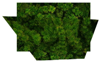Figure 7: Deformation during mosaicking produced by the wrong estimation through RANSAC for two images with low overlap.

1. RANSAC-1-OPT is performed. This is composed of the first modification of RANSAC (RANSAC-1) and the posterior optimization (OPT).

(a) RANSAC-1: The iteration counter cnt₁ is initialized with a value of zero, and the number of required iterations N with a value different from zero. The probability p_o of choosing a sample free of outlier is also initialized with a value of 0.99 as described in the original RANSAC method.

1. s = 4 matched points are randomly selected, from the sample space of S matches, so that these s matches are as distant as possible. These s matches are used to perform the initial estimation of the homography through the Direct Linear Transformation (DLT) algorithm. This allows that the estimated homography can project appropriately any set of points dispersed in the whole image, rather than just points located in one portion of the image. In order to find the most distant matched points, the matches were randomly paired and then the two most distant pairs of matched points where chosen. The fact that s = 4 is because it is the number of matches needed to estimate the homography H_o by using the DLT method.
2. Given the S homogeneous vectors x_c and x_c⁰ (representing the matches) and the estimated homography H_o, the solution of the minimization problem of (7) is a homography H_R that minimizes the symmetric transfer error for all the S The cost function of this minimization problem is the sum of the symmetric transfer error per match ste_c. Equation

(8) is used to calculate ste_c, where d(.) denotes the

Euclidean distance between two points.

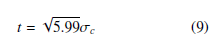
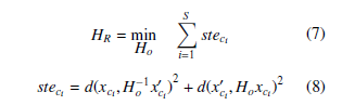iii. Using the homography H_R, the errors of each match with respect to the estimated model (the homography) are represented by the values of ste_c, so they are calculated by using (8). Then the standard deviation of those errors σ_c are computed. iv. The inliers of the model are represented by the homogeneous vectors x_inl and x_inl⁰ , and they are those matches whose values of ste_c are less than the threshold t, computed according to (9). Once the inliers are identified, it is also computed the number of inliers n_inl, the sum of symmetric transfer errors of the inliers STE_inl, and the standard deviation of the symmetric transfer errors of the

1. During the first iteration, the estimated homography H_R, the homogeneous vector of the inliers x_inl and x_inl⁰ , the number of inliers n_inl, the sum of symmetric transfer errors of the inliers STE_inl, and the standard deviation σ_inl, are save as reference for

the following iterations. For the rest of iterations, the following instructions are performed:

• If the calculated STE_inl is less than or equal to 10 times its reference, the reference will be updated with the calculated STE_inl, and then it will proceed with the next item.
• If the computed n_inl is greater than its reference, the reference for the values of H_R, n_inl, STE_inl, σ_inl, x_inl and x_inl⁰ will be updated with the computed values. Otherwise, it will proceed with the next item.
• If the computed n_inl is equal to its reference, the standard deviation σ_inl computed will be compared with the respective reference. If the calculated σ_inl is less than or equal to its reference, the reference values of H_R, n_inl, STE_inl, σ_inl, x_inl and x_inl⁰ will be updated with the computed values. Otherwise, it will proceed with the step 1-(a)-vi.

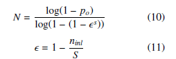
1. The iteration finishes and the iteration counter cnt₁ increases in 1. Then the number of required iterations N is computed adaptively based on the number of inliers n_inl. Equation (10) is used to make this calculation. The probability of choosing an outlier is calculated using (11).

• When the iteration counter cnt₁ would be greater than or equal to N, RANSAC-1 finishes and its outputs are the reference values for H_R, n_inl, STE_inl, σinl, xinl and xinl0 .
• OPT: The homography obtained after RANSAC-1 H_R is re-estimated utilizing just the n_inl homogeneous vectors representing the inliers x_inl and x_inl⁰ . The output is the homography H_e, which solve the minimization problem of (12). The cost function is the sum of the symmetric transfer error of all the inliers, presented in (13).

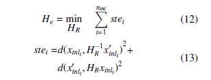• Given the estimated homography H_e and the inliers, (14) is used to calculate the percentage of inliers p_inl, and (15) is employed to compute the symmetric transfer error per inlier ste_inl.

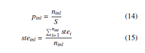
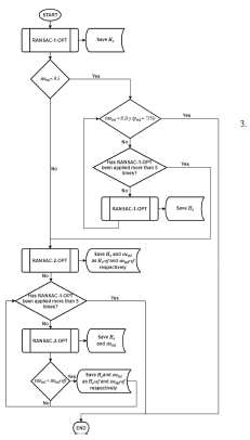Figure 8: Proposed algorithm for the automatic estimation of homographies.

2. If the ste_inl obtained in the step 1 is less than 0.5 pixels, it will proceed with the following item. It is important to mention that the value of 0.5 pixels was established after several tests of homography estimation between images with low overlap.
   • If the ste_inl is less than 0.2 and the p_inl obtained in the step 1 is greater than 75%, the estimated homography H_e will be the solution and the proposed method for automatic estimation of homography will end. Otherwise, it will proceed with the next item. The threshold value for the percentage of inliers p_inl was also established empirically.
   • RANSAC-1-OPT (described in the step 1) is applied again until the conditions of the previous item are satisfied, or until RANSAC-1-OPT has been applied 5 times in total. We applied continuously RANSAC-1OPT several times and we found that the result of the homography estimation did not improve after 5 times, so we established this threshold. If the solution is not found after applying RANSAC-1-OPT 5 times, it will proceed with the step 3.
3. RANSAC-2-OPT is performed. This is composed of the second modification of RANSAC (RANSAC-2) and the posterior optimization (OPT).
   • RANSAC-2: It initializes the same parameters of RANSAC-1 with the same values: the iteration counter cnt₂, the number of required iterations N, and the probability p_o of choosing a sample free of outlier.
     1. s = 4 matched points are randomly selected, from the sample space of S matches, to perform the initial estimation of the homography through the DLT algorithm. In this case, the matches are randomly selected without any other condition.
     2. Given the S homogeneous vectors x_c and x_c⁰ and the estimated homography H_o, the symmetric transfer error per match ste_c is computed using (8). The standard deviation of those errors σ_c is also computed.

• In the same manner as for RANSAC-1, the homogenous vectors of inliers x_inl and x_inl⁰ , the number of inliers n_inl, and the standard deviation of the symmetric transfer error of the inliers σ_inl are calculated.

1. During the first iteration, the estimated homography H_o, the homogeneous vector of the inliers x_inl and x_inl⁰ , the number of inliers n_inl, and the standard deviation σ_inl, are saved as reference for the following iterations. For the rest of iterations, the following instructions are performed:
   • If the computed n_inl is greater than the reference value of n_inl, the reference values of H_o, n_inl, σ_inl, x_inl and x_inl⁰ will be updated. Otherwise, it will proceed with the next item.
   • If the computed n_inl is equal to its reference, the standard deviation σ_inl computed will be compared with the respective reference. If the computed σ_inl is less than or equal to its reference, the reference values of H_o, n_inl, σ_inl, x_inl and ^x_inl⁰ will be updated with the computed values. Otherwise, it will proceed with the step 3-(a)-v.
2. The iteration finishes and the iteration counter cnt₂ increases in 1. Then the number of required iterations N is computed adaptively as it was done for RANSAC-1.
3. When the iteration counter cnt₂ would be greater than or equal to N, RANSAC-2 finishes and its outputs are the reference values for H_o, n_inl, σ_inl, x_inl and xinl0 .

• OPT: The homography obtained after RANSAC-2 H_o is re-estimated utilizing just the n_inl homogeneous vectors representing the inliers x_inl and x_inl⁰ . This is performed in the same way as performed in the step 1-(b), and the result is the homography H_e.
• Given the estimated homography H_e and the inliers, the percentage of inliers p_inl and the symmetric transfer error per inlier ste_inl are computed as it was done in the step 1-(c).

4. The homography H_e and the symmetric transfer error per inlier ste_inl obtained in the step 3 are saved as references H_e^ref and ste^ref_inl . Then, RANSAC-2-OPT is applied again and the calculated ste_inl is compared with the reference ste^ref_inl . If the calculated value is less than the reference, then the references H_e^ref and ste^ref_inl will be updated. This procedure is repeated 4 times.

The H_e^ref obtained after the repetitions is the solution and the proposed algorithm for the automatic estimation of the homography finishes.

An important detail of the implementation of RANSAC-1 and RANSAC-2 is the normalization of the homogeneous vectors of the matches. Before using these vectors for the homography estimation, it is required to normalize them; at the same time, denormalization must be performed after the homography estimation in order to maintain the original scale. Both normalization and denormalization improve the results by avoiding high errors during homography estimation.

The algorithm to calculate adaptively the number of iterations, the DLT algorithm, the normalization algorithm, and the original RANSAC algorithm are well developed in [17].

Once the homographies between two adjacent images in the same flight line are computed, the homographies between any image of the line and the central image (first image in the projection order) can be computed by multiplying homographies according to the sequence established and depicted in Figure 6b.

The homographies allow the computation of the location of images over the mosaic images, and then, the intensities of pixels are interpolated for the new positions. Merging all the projected images implies to find the intensity of pixel over the mosaic by averaging (or applying another similar procedure) the intensity of the same pixel in the projected images.

The new position of the images centers, and the position of the matches points between images of adjacent flight lines should be computed for each projected images through the homographies.

2.6         Image Mosaicking over mosaics of images acquired in the same flight line

This step of the proposed mosaicking method performs the image mosaicking of the mosaics obtained from images acquired in the same flight lines. The homographies between those individual mosaics are computed through the matches from images of adjacent lines. It proceeds as follows:

1. From the new positions of matches from images of adjacent lines, the matches from two adjacent mosaics X_m and X_m⁰ are computed.
2. The sequence of projection is determined in the same manner that was done for the images belonging to same flight lines (step 4^th) so the first image in the sequence is the mosaic image located in the middle.
3. The proposed algorithm for automatic estimation of homography (step 5^th) is applied to compute the homography between mosaic images.
4. The positions of the mosaic images in the whole mosaic is calculated, and the pixels information is interpolated for the new positions. This procedure is the same performed for individual images in the previous step (step 5^th).
5. The new positions of the images centers are computed by using the estimated homographies. Georeferencing requires the calculation of the new position of the images centers.

2.7        Georeferencing

In order to proceed with the georeferencing of the final mosaic, the position of the images centers as well as the UTM coordinates are required. The following steps detail this procedure:

1. The orientation of the Y-axis of the image is inverted to make possible align the image axes with the UTM coordinates axes through a rotation. Given the number of rows in the image M and the coordinates in Y-axis y, the new coordinates in the inverted Y-axis y⁰ are calculated by (16).

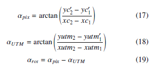
2. The angle between the image axes and the UTM coordinates axes α_rot, shown in Figure 9, is computed. Given the intrinsic coordinates (image coordinates) of the images centers belonging to the first two images in the projection order (Step 4^th) of the central line (xc₁, yc⁰₁), and (xc₂, yc⁰₂), and the UTM coordinates of the same images (xutm₁, yutm₁) and (xutm₂, yutm₂); the angle between the line that connect the centers of these two images and the X-axis of the image α_pix is calculated using (17). Besides, the angle between the line that connect the centers of these two images and the X-axis of UTM coordinate system α_UTM is computed using (18). The angle α_rot is computed using (19).

3. The image of the final mosaic is rotated −α_rot in the clockwise direction to align the axes of the image and the axes of the UTM coordinates.
4. After rotating the final mosaic image, the intrinsic coordinates of images centers will vary. Because of this, it is required to calculate these new rotated coordinates from the distances between centers of individual images and the center of the final mosaic, the rotated coordinates of the center of the final mosaic, and the rotated angle.
5. Linear regression is performed from the rotated coordinates of images centers and the UTM coordinates of the centers. Given the coordinates of images centers (xc, yc⁰), the UTM coordinates of the centers (xutm, yutm) can be expressed based on the coefficients of the linear regression a₁, a₂, a₃, a₄, a₅ and a₆ according to (20) and (21).

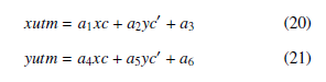6. The UTM coordinates of the four corners of the image are computed from (20), (21) and the coefficients a₁, a₂, a₃, a₄, a₅ and a₆.

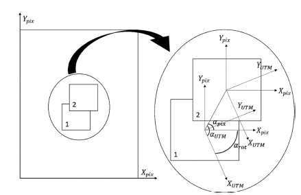Figure 9: Angle between the image axes and the axes of the UTM coordinates.

3. Results and Discussion

We describe the results of applying the proposed method over 6 sets of images acquired in 6 different flights regarding two scenarios: a city and a forest in Peruvian Amazon. These images were acquired with the professional camera Sony NEX-7, which allows taking images of 24.3MP, at a height of 100 meters from the ground. Each image possesses a spatial resolution of 6000x4000 pixels; but their sizes are reduced to a quarter of the original size during the processing, as it was explained in the first step of the proposed method.

The proposed method was implemented in MATLAB R2016a, and for validation purposes, we utilized the professional software Pix4DMapper Pro version 3.2.10, whose algorithm is based on Structure from Motion to generate 3D points and then orthorectified the mosaic as explained in [18]. We compared the processing time and the geolocation errors obtained in the same computer: HP Z820 Workstation with two processors Intel Xeon E5-2690 2.9GHz and 96 GB RAM. It is important to mention that the software Pix4DMapper Pro also processed the images resized to a quarter of the original size.

The processing time required to obtained each mosaic image is shown in Table 1. Pix4DMapper Pro performs a preprocessing step to calibrate images and it uses just the calibrated images for the image mosaicking; therefore, the processing time for this process is not included in our analysis.

Table 1: Processing Time

Flight	Number of images	Pix4DMapper Pro	Proposed Method
1	73	10 min 29 s	10 min 36 s
2	145	24 min 44 s	21 min 37.2 s
3	148	24 min 20 s	24 min 15 s
4	168	30 min 06 s	23 min 18 s
5	168	28 min 46 s	27 min 13.5 s
6	138	20 min 46 s	27 min 46 s

In addition, the geolocation errors corresponding to the UTM X-axis and the UTM Y-axis have been computed. From those errors, we calculate the mean absolute error (MAE) and the root mean square error (RMS) which are shown in Table 2.

Table 2: Geolocation Errors

Flight	Axes	Pix4DMapper Pro		Proposed Method
		MAE (m)	RMS (m)	MAE (m)	RMS (m)
1	X	0.9341	1.5209	1.2280	1.5942
	Y	3.7711	4.8955	3.4296	4.0248
2	X	1.9233	2.3048	2.5927	3.1386
	Y	4.3136	5.4267	4.0290	4.5155
3	X	2.2737	2.6818	3.4259	3.6941
	Y	4.6558	5.7388	8.1738	9.1930
4	X	4.2449	4.9988	3.9255	4.4720
	Y	3.7049	4.3406	3.1868	3.7808
5	X	3.6335	4.3212	4.4445	4.9658
	Y	3.8871	4.6748	2.8436	3.2852
6	X	0.8314	1.3360	1.7022	2.0033
	Y	4.6199	5.6286	3.7153	4.1984

From Table 1, we can observe that for flights 2, 3, 4 and 5 (corresponding to a forest in Peruvian Amazon), the proposed method was 6 minutes and 48 seconds faster in the best case, and just 5 seconds faster in the worst case. On the other side, for the flights 1 and 6, Pix4DMapper Pro was 7 minutes faster in the best case, and just 7 seconds faster in the worst case.

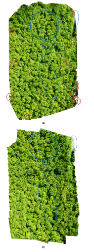Figure 11: Image mosaics obtained for the flight 6: (a) Pix4DMapper Pro (b) Pro

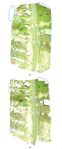Figure 10: Image mosaics obtained for the flight 1: (a) Pix4DMapper Pro (b) Proposed Method.

Regarding the MAE and RMS geolocation errors of the flights 1, 2, 5 and 6, the geolocation errors (both MAE and RMS) in X-axis computed with the proposed method were greater than those obtained by Pix4DMapper Pro; while, the geolocation errors in Y-axis computed with the proposed method were less than those obtained by Pix4DMapper Pro.

In the case of flight 3, MAE and RMS in both axes computed with our method were greater than those computed with Pix4DMapper Pro; but in flight 4, MAE and RMS in both axes computed with our method were less than those computed with Pix4DMapper Pro. For the majority of flights, the difference of both geolocation errors are low.

We observe that the geolocation errors computed with both methods in the Y-axis are always greater than the computed in the X-axis because of the employed GPS has that horizontal error distribution for all its measurements.

The highest differences in processing time and geolocation errors observed in Table 1 and Table 2 are because the inliers and the estimated homography for the same pair of images may produce different errors and different processing time. These differences are typical of the homography estimation step.

In Figure 10 and Figure 11, we compared the mosaic images obtained with Pix4DMapper Pro and our method for the flight 1 and 6 respectively. In the mosaic image of flight 1, regarding to a city, we can observe more clearly the differences between image mosaics. The image mosaic obtained by Pix4DMapper Pro presents some small holes in the boundaries of the image (indicated with red circles and ellipses). Besides, some trimmed edges and other differences caused by the enhancement of interpolated pixels information performed by Pix4DMapper Pro are encircled by blue ellipses. The mosaic image obtained with our method does not present holes and trimmed edges. For flight 6, the differences are not so clear as those of Figure 10 because it is difficult to see these differences in a scenario like a forest. Visible differences in Figure 11 are shown in the same way that was done for Figure 10.

4. Conclusions

The proposed method requires images acquired when the camera points the nadir, so an stabilization system or gimbal should be used. In this way, a mosaicking algorithm without any preprocessing (like the one performed in the algorithm of Pix4DMapper Pro) can be utilized to obtain good results. Otherwise, a more complicated algorithm should be used to perform the estimation of position and orientation of the cameras.

Finally, our mosaicking algorithm based on a simple process results being viable and reproducible to perform image mosaicking of aerial images for applications of natural resources monitoring because it obtains similar geolocation errors and processing time in comparison with a professional software based in Structure from Motion; moreover, our results do not present any holes or color incoherencies.

Conflict of Interest

The authors declare no conflict of interest.

Acknowledgment

We thank the National Innovation Program for Competitiveness and Productivity, Innovate Per´ u, for the funds´ allocated to our project (393-PNICP-PIAP-2014).

1.  A. Chaves, P. Cugnasca, J. Jose “Adaptive search control applied to Search and Rescue operations using Unmanned Aerial Vehicles (UAVs)” IEEE Latin America Transactions, 12(7), 1278–1283, 2014. https://doi.org/10.1109 8863
2.  A. Chaves, P. Cugnasca, J. Jose “Adaptive search control applied to Search and Rescue operations using Unmanned Aerial Vehicles (UAVs)” IEEE Latin America Transactions, 12(7), 1278–1283, 2014. https://doi.org/10.1109/TLA.2014.6948863
3.  J. Everaerts, “The use of Unmanned Aerial Vehicle (UAVS) for remote sensing and mapping” in 2008 XXI ISPRS Congress Technical Commission I: The International Archives of the Photogrammetry, Remote Sensing and Spatial Information Sciences. Vol. XXXVII Part B1, Beijing, China, 2008.
4.  Z. Li, V. Isler, “Large Scale Image Mosaic Construction for Agricultural Applications” IEEE Robotics and Automation Letters, 1(1), 295–302, 2016. https://doi.org/10.1109/LRA.2016.2519946
5.  A. Iketani, T. Sato, S. Ikeda, M. Kanbara, N. Nakajima, N. Yokoya “Video mosaicing based on structure from motion for distortion-free document digi- tization” in 2007 Computer Vision ACCV 2007. Lecture Notes in Computer Science. Vol. 4844, Tokyo, Japan, 2007. https://doi.org/10.1007/978-3-540- 76390-1 8
6.  Y. Yang, G. Sun, D. Zhao, B. Peng “A Real Time Mosaic Method for Re- mote Sensing Video Images from UAV” Journal of Signal and Information Processing, 4(3), 168–172, 2013. https://doi.org/10.4236/JSIP.2013.43B030
7.  T. Botterill, S. Mills, R. Green “Real-time aerial image mosaicing” in 2010 25th International Conference of Image and Vision Computing New Zealand, Queen- stown, New Zealand, 2010. https://doi.org/10.1009/IVCNZ.2016.6148850
8.  E. Garcia-Fidalgo, A. Ortiz, F. Bonnin-Pascual, J. Company “Fast image mo- saicing using incremental bags of binary words” in 2016 IEEE International Conference on Robotics and Automation (ICRA), Stockholm, Sweden, 2016. https://doi.org/10.1109/ICRA.2016.7487247
9.  D. Brito, C. Nunes, F. Padua, A. Lacerda “Evaluation of Inter- est Point Matching Methods for Projective Reconstruction of 3D Scenes” IEEE Latin America Transactions, 14(3), 1393–1400, 2016. https://doi.org/10.1109/TLA.2016.7459626
10. T. Kekec, A. Yildirim, M. Unel “A new approach to real-time mosaicing of aerial images” Robotics and Autonomous Systems, 62(12), 1755–1767, 2014. https://doi.org/10.1016/j.robot.2014.07.010
11.  Y. Xu, J. Ou, H. He, X. Zhang, J. Mills “Mosaicing of Unmanned Aerial Vehi- cle Imagery in the Absence of Camera Poses” Remote Sensing, 8(3), 204–219, 2016. https://doi.org/10.3390/RS8030204
12.  A. Moussa, N. El-Sheimy, “A fast approach for stitching of aerial im- ages” in 2016 XXIII ISPRS Congress, Commission III: The Interna- tional Archives of the Photogrammetry, Remote Sensing and Spatial In- formation Sciences. Vol. XLI Part B3, Prague, Czech Republic, 2016. https://doi.org/10.5194/isprsarchives-XLI-B3-769-2016
13. D. Lowe “Disctintive image features from scale-invariant keypoints” International Journal of Computer Vision, 60(2), 91–110, 2004. https://doi.org/10.1023/B:VISI.0000029664.99615.94
14.  A. Vedaldi, B. Fulkerson “VLFeat: An open and portable library of com- puter vision algorithms” in Proc. 18th International Conference on Multimedia,Firenze, Italy, 2010. https://doi.org/10.1145/1873951.1874249
15.  D. Del Castillo, E. Ota´rola, L. Freitas, Aguaje: the amazing palm tree of the Amazon, IIAP, Iquitos, Peru, 2006.
16.  L. Freitas, M. Pinedo, C. Linares, D. Del Castillo, Descriptores para el Aguaje (Mauritia flexuosa L. f.), IIAP, Iquitos, Peru, 2006.
17.  J. Levistre, J. Ruiz “El Aguajal: El bosque de la vida en la Amazon ́ıa Peruana” Ciencia Amazo´nica (Iquitos), 1(1), 31–40, 2011. https://doi.org/10.22386/ca.v1i1.6
18.  R. Hartley, A. Zisserman, Multiple view geometry in computer vision, 2th edition, Cambridge University Press, 2003.
19.  O. Ku¨ ng, C. Strecha, A. Beyeler, J. Zufferey, D. Floreano, P. Fua, F. Gervaix, “The accuracy of automatic photogrammetric techniques on ultra-light UAV im- agery” in International Conference on Unmanned Aerial Vehicle in Geomatics (UAV-g): The International Archives of the Photogrammetry, Remote Sensing and Spatial Information Scien es. Vol. XXXVIII Part C22, Zurich, Switzerland, 2011. https://doi.org/10.5194 22-125-2011

(Click Here)

(Click Here)