


1. Introduction
In situ measurements of glacier mass balance are rare at the global scale. The World Glacier Monitoring Service has compiled data from 110 of the ~100 000 existing glaciers listed in the World Glacier Inventory. To better understand the climate-glacier relationship at regional scale and to analyze the influences of both morphological (e.g. aspect, slope, elevation, latitude) and meteorological parameters (e.g. temperature, precipitation) on glacial changes, glaciological parameters (mass balance, equilibrium-line altitude (ELA)) at the scale of a mountain chain or a climatic region need to be measured. Remote-sensing techniques appear to be appropriate for this purpose (e.g. Reference ReesRees, 2006; Reference Bamber and RiveraBamber and Rivera, 2007).
The equilibrium line of a glacier separates the accumulation zone (where the annual mass balance is >0) from the ablation zone (where the annual mass balance is <0). Its position is determined by the climatological environment and the net budget for each individual year (Reference Meier and PostMeier and Post, 1962; Reference Kuhn and OerlemansKuhn, 1989). Reference LliboutryLliboutry (1965) stated that for midlatitude glaciers the position of the end-of-summer snowline, i.e. the snowline at the end of the hydrological year, can be considered as representative of the ELA. This assertion has since been confirmed for mid-latitude mountain glaciers (e.g. Reference Rabatel, Dedieu and VincentRabatel and others, 2005). This enables variations in the ELA to be reconstructed from remote-sensing data like aerial photographs and/or satellite images on which the snowline is generally easy to discern, and consequently study of the climate-glacier relationship in remote areas for which no direct measurements are available (e.g. Reference Chinn, Heydenrych and SalingerChinn and others, 2005; Reference Barcaza, Aniya, Matsumoto and AokiBarcaza and others, 2009). The relationship between the end-of-summer snowline and glaciological parameters also enables reconstruction of annual mass-balance time series, assuming that: (1) the mass-balance gradient in the vicinity of the ELA is representative of the mass-balance gradient of the whole glacier and remains constant throughout the study period; and (2) the average glacier mass balance over the study period has been determined using the geodetic method, which enables changes in volume to be computed by subtracting digital elevation models (DEMs) created by photogrammetry or field topography (e.g. Reference BraithwaiteBraithwaite, 1984; Reference Rabatel, Dedieu and VincentRabatel and others, 2005, 2008).
However, the above relationship is not valid for glaciers where superimposed ice (resulting from freeze/thaw cycles at the surface) is accreted to the glacier, which is the case for cold glaciers; in such cases, at the end of the hydrological year, the ELA is lower than the snowline altitude (SLA) (Reference Lliboutry, Williams and FerrignoLliboutry, 1998). For glaciers in the outer tropics, the representativeness of the snowline as an indicator of the ELA is still highly conjectural. The few studies performed in the outer tropical Andes that made use of this relationship assumed that the relationship is clear and comparable with that found in mid-latitude glaciers (e.g. Reference McFadden, Ramage and RodbellMcFadden and others, 2011; A. Klein and B. Isacks, unpublished information). On the one hand, it is known that most tropical glaciers are temperate (Reference Francou, Ribstein, Saravia and TiriauFrancou and others, 1995), so that the SLA-ELA relationship could be valid. However, previous glaciological studies in the outer tropical Andes have shown that: (1) the strong seasonality of precipitation, contrasting with the limited seasonality of temperature, generates a sequence of accumulation and ablation processes all year round that differs from those that take place in mid-latitude glaciers; and (2) tropical glaciers are characterized by a high mass-balance gradient mainly because of frequent changes in snow cover throughout the long ablation season (7–8 months) (e.g. Reference KuhnKuhn, 1984;Reference Sicart, Hock, Ribstein, Litt and RamirezSicart and others, 2011). For these reasons, the aim of this study was to test the validity of the SLA-ELA relationship for outer-tropical glaciers. We wanted to identify the most appropriate period of the year to measure the position of the snowline on glaciers in the outer tropics that could be considered representative of the equilibrium line. To this end, we first examined a 15year time series of monthly field mass-balance and ELA data on Glaciar Zongo to quantify their pattern of changes over the year. We then compared the SLAs computed for each year using remote sensing with the annual ELAs measured from field data to assess the validity of the SLA-ELA relationship for Glaciar Zongo and Glaciar Artesonraju in the outer tropics. The topic is important as it will help to improve our understanding of the climate-glacier relationship at the scale of a whole mountain range in the outer tropics.
2. Study Area, Climate Conditions and Glaciological Processes
Glaciar Zongo is located in the Bolivian Cordillera Real between the Altiplano plateau in the west and the Amazon basin in the east (Fig. 1a). In 2006, the glacier covered an area of 1.96km2 extending from 6100 to 4900 m a.s.l. (Reference SorucoSoruco and others, 2009). Glaciar Artesonraju is located in the Peruvian Cordillera Blanca (Fig. 1b). In 2003, the glacier covered an area of 5.39 km2 extending from 5980 to 4685 m a.s.l. (UGRH, 2010). Both Cordillera Real and Cordillera Blanca are situated in the outer tropical zone, which forms a transition zone between the tropics (continuously humid conditions) and the subtropics (dry conditions) (Reference KaserKaser, 2001).

Fig. 1. (a) Orthophoto map of Glaciar Zongo showing the surface topography in 1983, with 20m contour intervals, and the terminus of the glacier in 2006 (adapted from Reference SorucoSoruco and other, 2009). (b) Glaciar Artesonraju in 2010 (adapted from ©Google Earth).
The climate of the outer tropics is characterized by low seasonal temperature variability, high solar radiation influx all year round and marked seasonality of humidity and precipitation (Fig. 2) (e.g. Reference Wagnon, Ribstein, Francou and PouyaudWagnon and others, 1999). The hydrological year starts at the end of the dry season when discharge is minimal (fig. 2 of Reference SorucoSoruco and others, 2009), i.e. 1 September (Reference Ribstein, Tiriau, Francou and SaraviaRibstein and others, 1995). The hydrological year can be divided into three periods: (1) September- December, with a progressive increase in moisture and precipitation; (2) January-April, which is the core of the rainy season (approximately two-thirds of total annual precipitation); and (3) May-August, when conditions are dry (e.g. Reference Sicart, Hock, Ribstein, Litt and RamirezSicart and others, 2011). However, precipitation can also occur during the dry period due to Southern Hemisphere mid-latitude disturbances tracking abnormally north of their usual path (Reference RonchailRonchail, 1995; Reference Vuille and AmmannVuille and Ammann, 1997).

Fig. 2. Monthly precipitation and temperatures on Glaciar Zongo (in black) and Glaciar Artesonraju (in gray). Precipitation on Glaciar Zongo was recorded throughout 1995–2006 (the black boxes represent the monthly average of eight rain gauges located in the Glaciar Zongo watershed between 4750 and 5150 m a.s.l., and the vertical black bars represent the ±1σ interval between the eight rain gauges). The black line represents the monthly temperature recorded during 1995–2006 on the right-hand lateral moraine at 5150 m a.s.l.; the black vertical bars represent the ±1σ interval between the different years. Precipitation on Glaciar Artesonraju was recorded during 2002–04 (the gray boxes represent the monthly average of four rain gauges located in the Glaciar Artesonraju watershed between 4310 and 4935 m a.s.l., and the vertical gray bars represent the ±1σ interval between the four rain gauges). The gray line represents the monthly temperature recorded during 2001–04 on the left-hand lateral moraine at 4840 m a.s.l.; the grey vertical bars represent the ±1σ interval between the different years.
Reference Wagnon, Ribstein, Francou and PouyaudWagnon and others (1999, Reference Wagnon, Ribstein, Francou and Sicart2001) and Reference Sicart and Wagnon Pand RibsteinSicart and others (2005, Reference Sicart, Hock and Ribstein Pand Chazarin2010, Reference Sicart, Hock, Ribstein, Litt and Ramirez2011) studied seasonal variations in the melt rate of Glaciar Zongo using surface energy-balance methods. Here we only present a short summary of the main results; for more details the reader should refer to the abovementioned publications. Those authors showed that: (1) melt rates are highest in October-December, mainly as a result of ice melt due to solar radiation; (2) ablation remains high in January-April mainly due to snowmelt, with a decreasing trend toward the end of the period; and (3) from May to August ablation is limited because of significant energy losses due to longwave radiation, and consists mainly of sublimation because of strong winds and dry air, except at the glacier snout where melting can also occur as the elevation of the 0°C isotherm is very close to that of the snout. From May to August, the lower part of the glacier is usually snow-free and the snowline is high. However, any snowfall occurring in May-August will persist for a long time due to limited ablation. In such cases, the snowline is located close to the glacier snout and may remain in that position throughout the dry season.
3. Methods and Data
3.1 Mass balance and ELA computed from direct field measurements
The mass balance of Glaciar Zongo has been monitored since 1991 using the glaciological method (Reference PatersonPaterson, 1994). On the lower part of the glacier (<5200 m a.s.l.), stake emergence is measured at monthly intervals using a network of 10–25 stakes (Fig. 1a). The number of stakes can vary from one month to another, as stakes can be lost, broken or covered by snow. Snow height and density measurements are required together with stake emergence measurements because snowfall can occur on the glacier surface at any time of the year. On the upper part of the glacier, net accumulation (snow height and density) is measured at the end of the hydrological year, i.e. in late August of each year, at three locations (Fig. 1a). To compute the monthly mass balance of Glaciar Zongo, the accumulation measurements were distributed at a monthly timescale using monthly precipitation data measured on a network of five rain gauges located on the glacier foreland between 4830 and 5150 m a.s.l. (Fig. 1a), assuming that monthly variability is identical. Finally, to compute the specific mass balance of the glacier, its hypsometry was calculated using digital elevation models (DEMs) computed from aerial photogrammetry in 1983, 1997 and 2006 (Reference SorucoSoruco and others, 2009;Section 3.2 below).
The ELA of Glaciar Zongo was calculated for each year between 1991 and 2006 using the stake measurements made on the lower part of the glacier. For each year, the mass balance of each stake was cumulated monthly from September to August. Then, for each month, the linear regression of mass balance with stake altitude was used to calculate the ELA (Fig. 3). ELA uncertainty was calculated from the standard error of the linear regression of the mass balance with stake altitude.

Fig. 3. Measured mass balance as a function of elevation of the stake network located in the lower part of Glaciar Zongo (each dot represents one stake) for three contrasted years: 1996/97 (squares), a positive mass-balance year; 1997/98 (triangles), a very negative mass-balance year; and 2005/06 (diamonds), an almost balanced year.
On Glaciar Artesonraju, field mass-balance measurements have been made since 2000 using a stake network distributed throughout the ablation zone up to ~4850m a.s.l. These measurements are made at a varying timescale of ~3 months. Since 2004, accumulation measurements have also been made once a year (at the end of the dry season), enabling the specific mass balance of the glacier to be computed. The ELA of Glaciar Artesonraju was calculated for each year between 2000 and 2010, using the stake measurements made on the lower part of the glacier.
3.2. Satellite images and DEM description
Landsat-5 Thematic Mapper (TM), Landsat-7 Enhanced TM Plus (ETM+) and Systéme Pour l’Observation de la Terre (SPOT 4) images were used for this study. No Advanced Spaceborne Thermal Emission and Reflection Radiometer (ASTER) image was used because, among the available images, the only images with satisfactory cloudiness conditions were acquired on the same day as the Landsat images. These sensors are appropriate for the purpose of our study as they are of high spatial resolution: 15 and 30 m for Landsat, 10 and 20m for SPOT in the panchromactic and multi- spectral modes, respectively.
One limitation of optical satellites such as Landsat, SPOT or ASTER is the cloud cover. For both the Cordillera Real, Bolivia and Cordillera Blanca, Peru, the high cloudiness at the onset and during the core of the rainy season (Septem-ber-April) precludes the use of images acquired during this period of the year. Consequently, the time of year when images can be used is limited to the dry season, i.e. from late April/early May to late August/early September. Another limitation is the temporal resolution with a repeat cycle ranging from 16 to 26days depending on the satellite.
For Glaciar Zongo, of the 55 Landsat images available on the Global Visualization Viewer (GLOVIS) of the United States Geological Survey-EROS Data Center (USGS-EDC) for the period 1991–2006, conditions were satisfactory in 29 images. All the Landsat images were provided with systematic radiometric and geometric corrections (http://land- sat.usgs.gov/Landsat_Processing_Details.php). As no image was available between 1991 and 1995, we reduced our study period to 1996–2006. Fortunately Glaciar Zongo is located at the center of the Landsat images and was consequently not affected by the failure of the Landsat-7 scan-line corrector on 31 May 2003.
To complete the Landsat image series for Glaciar Zongo, three SPOT images were obtained through the French Space Agency (CNES)/Spot-Image ISIS program (Table 1). The SPOT images were geometrically corrected and georeferenced on the basis of the Landsat images using the commercial PCI Geomatics® software. The root-mean-square error in longitude and latitude (RMSExy) at the ground-control points used for the geometrical correction is <1 pixel.
Table 1. Satellite images used for SLA measurements. For Landsat-5 TM (LT5) and Landsat-7 ETM+ (LE7) images, the path/row was 001/070 for Glaciar Zongo and 008/066 for Glaciar Artesonraju; the pixel size was 15 and 30 m for the panchromatic and multispectral modes, respectively. For the SPOT images used for Glaciar Zongo, the path/row was 668/382 or 668/383 and the pixel size was 10 m for the panchromatic mode (PAN) and 20 m for the multispectral mode (XS)

For Glaciar Artesonraju, of the 49 Landsat images available on GLOVIS for the period 2000–10, conditions were satisfactory in 30. As for Glaciar Zongo, all the Landsat images were provided free of charge by the USGS including systematic radiometric and geometric corrections.
Once the snowline was identified on the satellite images, its average altitude was calculated using a DEM. For Glaciar Zongo, the DEM was computed photogramme- trically using 2006 aerial photographs from the National Service of Aerophotogrammetry, Bolivia (see Reference SorucoSoruco and others (2009) for details of the construction of this DEM). The horizontal and vertical accuracies of this DEM are 1.38 and 3.50 m, respectively. Using the geodetic method, Reference SorucoSoruco and others (2009) showed that at the level of the mean ELA (~5150 m a.s.l., which is the average of the annual ELAs for the period 1991–2006 computed from field measurements), Glaciar Zongo lost about 20 m between 1997 and 2006. Thus, to compensate for the fact that the DEM used to compute the SLAs dates from the end of the study period (2006), the SLA for each year was corrected considering a linear trend of surface lowering of 2 m a-1. For Glaciar Artesonraju, because no DEM was computed from aerial photogrammetry, the DEM used to compute the altitude of the snowline identified on the satellite images was the ASTERGDEM V2, the vertical accuracy of which is ~20m (http://www.ersdac.or.jp/GDEM/E/4.html). With such vertical accuracy, there was no need to undertake altitudinal correction of the SLA as for Glaciar Zongo, because the accuracy is of the same order of magnitude as the surface lowering.
3.3. SLA retrieved from satellite images
Since the first optical satellite images from the Landsat program became available in 1972, several methods have been developed to monitor the properties of glaciers including ice extent, terminus position, surface elevation and the position of the snowline. Several compilations of these techniques have been published in review papers and books (e.g. Reference MeierMeier, 1980; Reference ReesRees, 2006). For snowline delineation, we advise the reader to consult the abovementioned references for an extensive description of the different methods corresponding to the potential of each satellite.
Figure 4 shows the results of a test of different band combinations and band ratios recommended in the abovementioned references to facilitate the identification of the snowline on the satellite images. Case F turned out to be the most appropriate, as the limit between snow (light blue) and ice (black) is clearly visible. This case combines the green, near-infrared and shortwave infrared bands with thresholds for the green and near-infrared bands. The thresholds depend on lighting conditions on the acquisition date. For the Landsat images listed in Table 1, the spectral bands used were 2 (0.52–0.60 µm), 4 (0.77–0.90 µm) and 5 (1.551.75 µm), and the thresholds ranged between the digital number values of 80 and 160 for band 2 and between 60 and 135 for band 4. For the SPOT multispectral images, spectral bands 1 (0.50–0.59 mm), 3 (0.79–0.89 mm) and 4 (1.58–1.75 mm) were used.

Fig. 4. Test of different combinations of bands and band ratios applied on Landsat-5 image acquired on 2 July 1999 to facilitate the identification of the snowline: (a) combination of spectral bands 3, 2 and 1; (b) ratio 3/5; (c) ratio 4/5; (d) normalized-difference snow index (NDSI) with threshold at 0.6; (e) combination of spectral bands 5, 4 and 2; (f) same as (e) with threshold of 120 and 135 for bands 4 and 2, respectively. In (f) the yellow arrow shows the position of the snowline on Glaciar Zongo.
Uncertainty was estimated for each SLA. Uncertainty results from different sources of error (Reference Rabatel, Dedieu and ReynaudRabatel and others, 2002, 2005): (1) the pixel size of the images, which ranges between 10 and 30 m depending on the sensor;(2) the slope of the glacier in the vicinity of the SLA, which ranges between 12% and 49% depending on the zone where the SLA was located in the year concerned; (3) the accuracy of the DEM (3.5 and 20.0 m for Glaciar Zongo and Glaciar Artesonraju, respectively); and (4) the standard deviation of the calculation of the average SLA along its delineation, which ranges between 10 and 80 m depending on the year. The latter source of error was the most important. The resulting total uncertainty on the SLAs (root of the quadratic sum of the different independent errors) varied between ±11 and ±86 m depending on the year. The uncertainty is greater when the SLA is located in the upper part of the glacier because the slope is steeper there and the standard deviation of the computed SLA is larger.
4. Results and Discussion
4.1. Changes in monthly mass balance and ELA over the year
Figure 5a shows the mass balance cumulated at a monthly timescale from September to August on Glaciar Zongo. From 1991 to 2006, the centered monthly mass balance was negative, except between January and March when accumulation was maximal. The most negative mass-balance values were recorded in November, i.e. before the core of the rainy season. Monthly variability of the mass balance was highest in October-December due to the variability of the onset of the rainy season. Indeed, the later the rainy season begins, the longer the period with the highest ablation rates (Reference Sicart, Hock, Ribstein, Litt and RamirezSicart and others, 2011). Reference SorucoSoruco and others (2009) showed that the variance of the mass-balance time series of the lower part of the glacier (z <5200 m a.s.l.), where the mass balance is measured directly from the stake network, was responsible for 80% of the interannual variability of the mass balance of the whole glacier.

Fig. 5. Cumulated monthly mass balance and ELA of Glaciar Zongo from September to August (average values for the period 1991–2006). (a) The mass balance is centered and cumulated monthly (thick black line). Gray lines represent cumulated variability for the whole year. (b) Black diamonds represent the average ELA for the study period, with uncertainty bars matching the ±1σ interval. Gray squares and triangles represent the two extreme ELA patterns for 1997/98 and 2000/01, respectively.
Along with changes in the monthly mass balance, Figure 5 shows changes in the monthly ELA on Glaciar Zongo during the study period: (1) the ELA increased progressively from September to November due to increasing ablation rates that reached their peak around November; (2) the ELA reached maximum around November, but with marked year-to-year variability; (3) the ELA decreased from December to April due to frequent snowfalls on the glacier; and (4) the ELA increased again over the dry season from May onwards, but this increase (20m on average between April and August during our study period) was limited due to low ablation rates. The average annual ELA on Glaciar Zongo for the study period was 5144±67ma.s.l.
As mentioned in Section 2, discharge is minimal in July- August. The glaciological mass balance was calculated for the same period as the hydrological mass balance (Reference Ribstein, Tiriau, Francou and SaraviaRibstein and others, 1995), i.e. from 1 September to 31 August, and not at the end of the strongest ablation period (November in our case) as is the case for mid-latitude glaciers. As a consequence, and because changes in the mass balance and ELA are very low between May and August, the cumulated monthly mass balance and the position of the equilibrium line at the end of the wet season, i.e. in April, account for the accumulation and ablation processes that mainly control the annual mass balance. One consequence of these changes in the mass balance and ELA over the hydrological year is that if one wishes to use the snowline measured on satellite images as an indicator of the annual equilibrium line, and thus of the annual mass balance, it is best to use satellite images acquired between May and August.
4.2. Comparison of ELA and SLA
Figure 6 compares the SLAs computed from the satellite images with the annual ELAs computed from field mass balance for both Glaciar Zongo and Glaciar Artesonraju for the corresponding years. Each dot corresponds to one image. Note that for several years, four or five images acquired between May and August were available (e.g. 1996/97 and 1997/98 for Glaciar Zongo), but for other years only one image was available (e.g. 1995/96 or 2000/01 for Glaciar Zongo; see also list of images in Table 1). When several images were available for a given year, there is considerable scatter between the image data. The scatter was computed as the difference between the lowest and highest SLAs measured on the available images for each year. This varied between 7 and 236 m, with an average of 77 m, for Glaciar Zongo and between 26 and 73 m, with an average of 44 m, for Glaciar Artesonraju. However, regardless of the year, the highest SLA was usually close to the 1: 1 diagonal, suggesting that the highest remotely sensed SLA is a good indicator of the annual ELA. However, for a few years, the SLA on Glaciar Zongo was significantly below the ELA. This was the case for 1995/96, 1998/99, 2000/01 and 2001/02. In these cases, the glacier tongue was almost completely covered by snow when the image was acquired (SLA <5000ma.s.l.) due to snowfalls that occurred in the dry season.

Fig. 6. Comparison of the annual ELA calculated from field mass-balance measurements and SLAs computed from all the available satellite image acquired in May-August of the corresponding year for each year of the study period. Each dot corresponds to one image. Uncertainty bars match the ±1σ interval. The pale gray line matches the 1:1 diagonal.
Furthermore, the highest SLA was not necessarily concomitant with the end of the hydrological year, i.e. late August, but could occur in May, June or July. For example, in 1997/98, the highest SLA was measured on the Landsat image dated 13 June, while the SLA measured on the Landsat image dated 31 July was about 240 m lower.
One could argue that an alternative method is to measure the SLA on all the available satellite images and take the highest one, but even proceeding in that way there is no guarantee that the SLA is representative of the ELA. For example, if on all the available images for a given year the major part of the glacier appears to be covered with snow due to snowfalls that occurred in the days preceding the acquisition of the images by the satellite, none of the SLAs computed from these images would be representative of the ELA. Thus, the comparison of the highest SLA measured on the available satellite images with the ELA computed from field data of a benchmark glacier is the only way to be sure that the SLA is representative of the ELA. For validation, this comparison is an essential step before taking SLA measurements on other glaciers on the same image for which no field data are available.
Figure 7 compares the annual ELA with the highest SLA for the period May-August computed using satellite images of Glaciar Zongo acquired in 1996–2006 and of Glaciar Artesonraju acquired in 2000–10. The correlation was significant at the 99% confidence interval (r2 = 0.84 for Glaciar Zongo and r2 = 0.89 for Glaciar Artesonraju). The average difference between the SLA and the annual ELA for each year of the study period was about –32 m for Glaciar Zongo and about –10 m for Glaciar Artesonraju. For Glaciar Zongo, the biggest difference was observed in four years: 1995/96, 1998/99, 2000/01 and 2001/02. Figure 7 shows that for these years, even considering the uncertainty bars on the SLA values, there was no overlap with the 1: 1 diagonal. Removing these values, the correlation increased (r2 = 0.98) and the average difference between the SLA and the ELA for each year over the study period decreased to –7 m. For these years, the SLA computed from satellite images underestimated the ELA. This was because snow covered the glacier tongue in June or July. Figure 8 shows daily precipitation recorded at ‘La Plataforma’ (4800 m a.s.l.), about 1 km from the snout of Glaciar Zongo, for 1995/96, 1998/99, 2000/01 and 2001/02. The vertical red lines indicate the dates of the satellite images available for each of the years concerned. In May-August, precipitation at La Plataforma was almost exclusively in solid form. This was also the case on the glacier, which is located 100 m higher (e.g. Reference Wagnon, Ribstein, Francou and PouyaudWagnon and others, 1999). Considering each of these years individually, only one image was available for two of them (1995/96 and 2000/01). In both cases, precipitation events occurred within the 15 day period before the image was acquired (~15 mm w.e. in 2 days for 1995/96 and ~16mmw.e. in 5 days for 2000/01) and because the ablation is almost negligible at this period of the year, snow still covered the glacier surface. For 1998/99 and 2001/02, although several images were available, precipitation events also led to a low SLA.

Fig. 7. Comparison of the highest remote-sensed SLA for each year and the annual ELA of the corresponding year for Glaciar Zongo (1996–2006) and Glaciar Arstesonraju (2000–10). Error bars match the uncertainties in the ELA and SLA measurements.
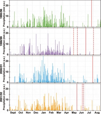
Fig. 8. Daily precipitation (mmw.e.) for the years 1995/96, 1998/99, 2000/01 and 2001/02 recorded at ‘La Plataforma’ (4800ma.s.l.) located ~1 km from the snout of Glaciar Zongo. The vertical red lines show the dates of the satellite images available for each of the years.concerned: solid lines show the image for which the SLA is closest to the ELA, and dashed lines show the other images. At this elevation, precipitation may fall in liquid form between November and March, but falls almost exclusively in solid form between May and August.
Figure 9 compares the annual mass balance with the highest SLA of the corresponding year for Glaciar Zongo. Even assuming that the SLA values in the four years discussed above are too low and that the mass-balance gradient on Glaciar Zongo is high at the glacier snout and decreases with altitude, the correlation was significant at the 99% confidence interval (r2 = 0.84). We thus conclude that, for our study period, these SLAs are good indicators of the annual mass balance of the glacier. This in an important finding for the reconstruction of annual mass-balance time series on the basis of SLA measurements by remote sensing, which is one possible application of the method developed by Reference Rabatel, Dedieu and VincentRabatel and others (2005, Reference Rabatel, Dedieu, Thibert, Letreguilly and Vincent2008) in the outer tropical Andes. This will be the topic of a forthcoming publication.

Fig. 9 Comparison of the highest remote-sensed SLA for each year and the annual mass balance of the corresponding year for Glaciar Zongo (1996–2006). Error bars match the uncertainties on the mass balance and SLA measurements.
5. Summary and Concluding Remarks
One advantage of using satellite images in glaciology is being able to measure the position of the snowline as an indicator of the equilibrium line on glaciers for which no direct field measurements are available. Although the representativeness of the snowline as an indicator of the ELA is well known for mid-latitude glaciers, the relationship between these two parameters had been poorly studied in the outer tropics. In this study, we have shown that:
-
1. Changes that occur during the dry season (May-August) in both the ELA computed from field measurements and in the SLA computed from satellite images are very limited because of the low melt rates. Consequently all satellite images acquired between May and August can be used to compute the SLA representative of the ELA for glaciers in the outer tropics.
-
2. Choosing the highest SLA detected on different satellite images acquired during the dry season makes it possible to obtain a good estimate of the ELA. However, as snowfall events can also occur during the dry season, the SLA detected on satellite images tends to underestimate the ELA. As a consequence, the validity of the SLA computed from satellite images with field data collected on a benchmark glacier has to be checked before measuring the SLA on other glaciers in the same mountain range visible in the images.
In this context, field measurements made on several tropical glaciers of the Andes (Cordillera Real, Bolivia; Cordillera Blanca, Peru; Cordillera Central, Ecuador) by the GLACIO- CLIM Observatory and local institutions, such as the Universidad Mayor de San Andres (UMSA), Bolivia, the Unidad de Glaciologfa y Recursos Hfdricos (UGRH), Peru and the Instituto Nacional de Meteorologla e Hidrologla (INAMHI), Ecuador, are very valuable and it is crucial to maintain such monitoring networks in the long term.
Once the relationship between the SLA and the ELA has been validated, the satellite images can be used to measure the snowline on other glaciers visible in the images in order to reconstruct mass-balance time series and to quantify the sensitivity of mass balance to climate and morphological parameters at the scale of a mountain area or a climatic region. These reconstructions of annual mass-balance time series will be the topic of a forthcoming publication.
Acknowledgements
We are grateful to all those who took part in field campaigns to measure mass balances on Glaciar Zongo (especially Rolando Fuertes) and Glaciar Artesonraju. We thank the USGS-EDC for allowing us free access to Landsat images. SPOT images were provided through the CNES/SPOT-Image ISIS program, contract No. 503. This study was funded by the French IRD (Institut de Recherche pour le Développement) through the ‘Glaciers Observatory’: GLACIOCLIM (http://www-lgge.ujf-grenoble.fr/ServiceObs/SiteWebAndes/index.htm). Comments from two anonymous reviewers helped us to improve the paper.


