New insights into the biennial-to-multidecadal variability of the water level fluctuation in Lake Titicaca in the 20th century
 Juan Sulca
 James Apaéstegui
 José Tacza
- 1Instituto Geofísico del Perú, Lima, Peru
- 2Programa de Maestria en Recursos Hídricos, Universidad Nacional Agraria La Molina, Lima, Peru
- 3Institute of Geophysics, Polish Academy of Sciences, Warsaw, Poland
- 4HUN-REN Institute of Earth Physics and Space Science, Sopron, Hungary
- 5Center of Radio Astronomy and Astrophysics Mackenzie, Engineering School, Mackenzie Presbyterian University, Sáo Paulo, Brazil
The water disponibility of Lake Titicaca is important for local ecosystems, domestic water, industry, fishing, agriculture, and tourism in Peru and Bolivia. However, the water level variability in Lake Titicaca (LTWL) still needs to be understood. The fluctuations of LTWL during the 1921–2018 period are investigated using continuous wavelet techniques on high- and low-pass filters of monthly time series, ERA-20C reanalysis, sea surface temperature (SST), and water level. We also built multiple linear regression (MLR) models based on SST indices to identify the main drivers of the LTWL variability. LTWL features annual (12 months), biennial (22–28 months), interannual (80–108 months), decadal (12.75–14.06 years), interdecadal (24.83–26.50 years), and multidecadal (30–65 years) signals. The high- and low-frequency components of the LTWL are triggered by the humidity transport from the lowland toward the Lake Titicaca basin, although different forcings could cause it. The biennial band is associated with SST anomalies over the southeastern tropical Atlantic Ocean that strengthen the Bolivian High-Nordeste Low system. The interannual band is associated with the southern South Atlantic SST anomalies, which modulate the position of the Bolivian High. According to the MLR models, the decadal and interdecadal components of the LTWL can be explained by the linear combination of the decadal and interdecadal variability of the Pacific and Atlantic SST anomalies (r > 0.83, p < 0.05). In contrast, the multidecadal component of the LTWL is driven by the multidecadal component of the North Atlantic SST anomalies (AMO) and the southern South Atlantic SST anomalies. Moreover, the monthly time series of LTWL exhibits four breakpoints. The signs of the first four trends follow the change of phases of the multidecadal component of LTWL, while the fifth trend is zero attributable to the diminished amplitude of the interdecadal component of LTWL.
1 Introduction
During Austral summer (December-January-February, DJF), the maximum precipitation falls over the south-central Amazon, and the northwest-southeast oriented South Atlantic Convergence Zone (SACZ) produces a cloud band with enhanced precipitation that appears to merge with the intense convection over the Amazon Basin, extending from tropical South America southeastward into the South Atlantic Ocean (Kodama, 1992; Liebmann et al., 1999; Grimm, 2019). At low levels, the South American low-level jet (SALLJ) transports warm and moist air from the Amazon basin toward the subtropics along the eastern flank of the Andes Mountains (Jones, 2019; Montini et al., 2019). In the upper troposphere, the Bolivian High and Nordeste Low (BH–NL) system is the main feature over South America at 200 hPa (Chen et al., 1999). The latent heat released during convection over the Amazon basin determines the fundamental structure of the BH–NL system (Lenters and Cook, 1995, 1997). Moreover, Chen et al. (1999) also found that the tropical-subtropical sea surface temperature (SST) anomalies of the southeastern tropical Atlantic Ocean strength the intensity of the BH-NL system (Chen et al., 1999). The BH–NL system, however, disappears during austral winter once the upper-level westerly zonal flow is established over South America.
The Central Andes is located within Andes Mountains between 10°S and 30°S, and its mean maximum height exceeds 5,000 m. The precipitation in the Central Andes presents a rainy season between December and February, while the dry season occurs from June to August (Garreaud et al., 2003; Imfeld et al., 2019). The wet seasons in this region are caused by the upper-level easterly flow that induces humidity transport from the Amazonia to the central Andes (Garreaud et al., 2003; Vuille and Keimig, 2004). However, the negative relationship between precipitation and upper-level zonal wind at 200 hPa started weakening in the 2000s because of the remote effect of the deep convection over the northwestern Peruvian Amazon (Segura et al., 2020).
The Lake Titicaca basin (LTB) is located in the Altiplano region between Peru and Bolivia at 68°33′−70°1'W and 15°6′−16°50'S with an average altitude of 3,810 m (Figure 1A). The total surface area of LTB is 8,560 km2. LTB presents a population of around 1 273 014 habitants (Ministerio del Ambiente, 2013). Lake Titicaca (8,500 km2) is the highest (~3,809 m) navigable lake in the world (Figure 1A). The water disponibility of Lake Titicaca is important for local ecosystems, domestic water, and various economic activities, such as industry, fishing, agriculture, and tourism (Hastenrath and Kutzbach, 1985; Chura-Cruz et al., 2013; Canedo et al., 2016).
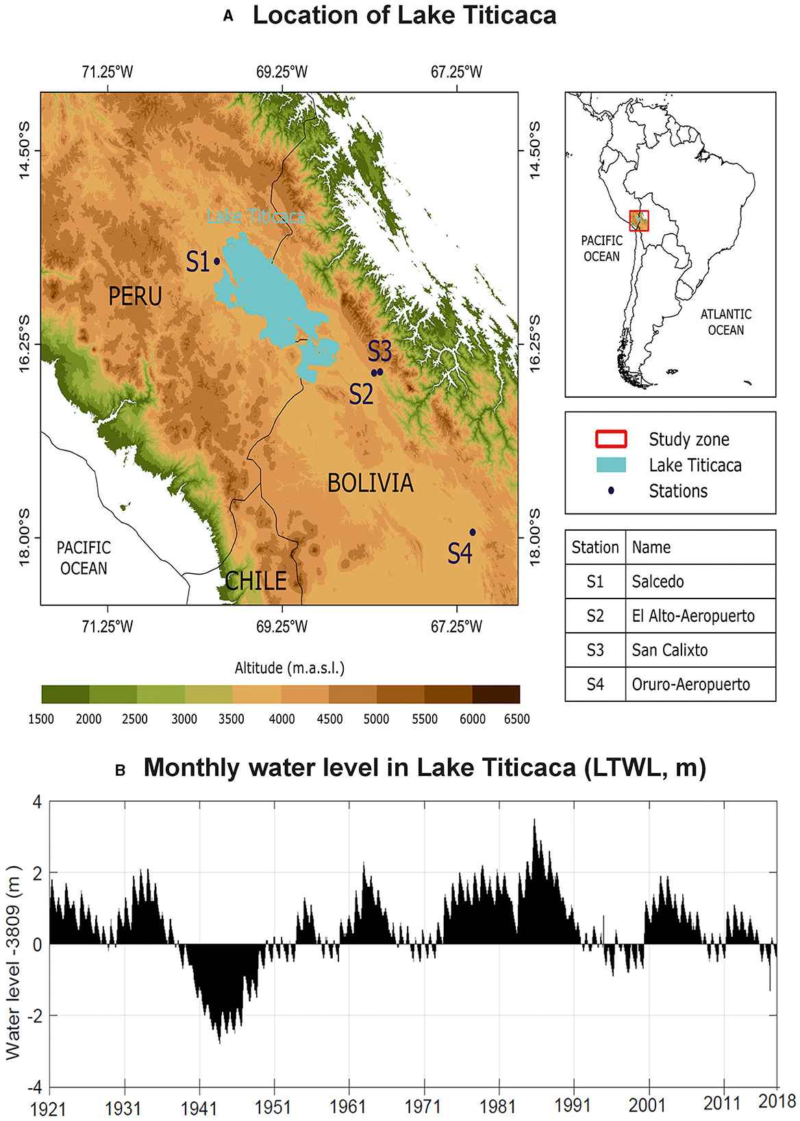
Figure 1. (A) Location of Lake Titicaca within South America. (B) Monthly time series of water level (m month−1) in the Lake Titicaca. The analysis is based on the 1921–2018 period. (A) Location of Lake Titicaca. (B) Monthly water level in Lake Titicaca (LTWL, m).
Lima-Quispe et al. (2021) highlight that the climate controls the fluctuation of Lake Titicaca water level (LTWL). For example, the climate explains about 80% of the fluctuation in Lake Titicaca, while the irrigation explains the remaining 20%. Ronchail et al. (2014) pointed out that the range of extreme LTWL variation in 1915–2009 was approximately 5 m, from 3,806.7 m in 1944 to 3,811.6 m in 1986 (Figure 1B). Sztorch et al. (1989) documented that the heavy precipitation in 1985/86 caused the highest LTWL, greatly damaging the local population. Figure 2 shows that LTWL presents a well-defined annual distribution, where the maximum (minimum) water levels occur between March and May (November and January). The annual cycle of the LTWL also features a negative lag of 3 months (December–February) with the annual precipitation cycle in the Bolivian Altiplano.
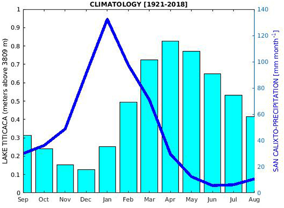
Figure 2. Monthly climatology of precipitation (in mm month−1; bold blue line) in San Calixto station and water level (in m month−1; cyan bars) in Lake Titicaca. San Calixto station covers the 1930–1990 period. The monthly record of the water level in Lake Titicaca covers 1921–2018 period, considering the reference lake level is 3809 m.
Several studies have predicted a decrease in precipitation over the Altiplano region by the end of the 21st century (Urrutia and Vuille, 2009; Minvielle and Garreaud, 2011; Neukom et al., 2015; Vera et al., 2019; Sulca and da Rocha, 2021; Zubieta et al., 2021). Based on the linear relationship between precipitation (PRE) and 200 hPa zonal wind (U200) anomalies in the current climate, a significant reduction in austral summer precipitation over the central Andes, ranging from 10% to 30%, is projected by the end of this century under the A2 scenario belongs to AR4 (Intergovernmental Panel on Climate Change, IPCC) (Minvielle and Garreaud, 2011). Nevertheless, it is important to exercise caution with this projection, as the PRE-U200 relationship over the central Andes began weakening in 2000 (Segura et al., 2020). Using a multimodel ensemble consisting of five models (EC-EARTH, HadGEM2-ES, IPSL-CM5A-LR, MIROC5, and MPI-ESM-LR) out of 31 from the Coupled Multimodel Intercomparison Phase 5 (CMIP5), Zubieta et al. (2021) observed that the Lake Titicaca basin indicates an increase in austral summer precipitation of <8.2% for the period 2034–2064 compared to 1984–2014 under the Representative Concentration Pathways 8.5 (RCP 8.5) scenario. Sulca and da Rocha (2021) employed regional climate simulations and identified a relative precipitation reduction of −10% projected for the central and southern parts of the central Andes. Centro de Ciencia del Clima y la Resilencia (CR)2 (2018) reported a similar projected precipitation reduction using statistical downscaling models that rely on fine-resolution simulations from regional climate model version 4 (RegCM4). However, there has been no study on the future projections of water level trends in Lake Titicaca using coupled global models from the CMIP Project.
The SST anomalies of the Pacific and Atlantic Oceans present high- and low-frequency components. The intraseasonal, seasonal, annual, interannual, and biennial components form the high SST variability. Low SST variability groups the decadal, interdecadal, and multidecadal components.
On intraseasonal timescales, the Madden–Julian Oscillation (MJO) is observed as an intraseasonal phenomenon. The MJO is a large-scale, anomalous atmospheric circulation pattern that originates in the western Indian Ocean and is restricted to tropical regions. It is characterized by eastward propagation at speeds ranging from 5 to 10 m s−1. The MJO exhibits periods ranging from 30 to 90 days (Madden and Julian, 1972, 1994) and reaches its maximum intensity twice a year: during the Southern Hemisphere's summer and autumn. This wave disturbance is characterized by eastward propagation of tropical convective anomalies from the Indian Ocean to the western Pacific, extending further to South America and Africa. Numerous studies have investigated the influence of the MJO on extreme rainfall events in the South American continent (Madden and Julian, 1972; Alvarez et al., 2016; Mayta et al., 2019; Recalde-Coronel et al., 2020; Fernandes and Grimm, 2023). In the central Andes, both moisture and precipitation in the Altiplano region exhibit intraseasonal variability (Garreaud, 2000; Falvey and Garreaud, 2005; Sulca, 2023). Garreaud (2000) highlighted the presence of an intraseasonal signal in summer rainfall over the Altiplano region, associated with an upper-level easterly zonal flow anomaly. Falvey and Garreaud (2005) documented that the intraseasonal variation in humidity flux from the Amazon basin to the Altiplano region accounts for intraseasonal precipitation variability in this region. Recently, Sulca (2023) reported that the MJO influences summer precipitation in the Altiplano region on intraseasonal timescales. However, there has been no study on the influence of the MJO on water level fluctuations in Lake Titicaca.
Concerning biennial timescales, Sulca et al. (2022a) discovered that the summer SST anomalies in the Western Pacific (Niño 4) and the Central Pacific exhibit a biennial component with a period of 2.5 years. The tropical South Atlantic and North Atlantic display a biennial component with a periodicity ranging from 2.1 to 2.2 years. Some studies have proposed the presence of a biennial signal in Altiplano precipitation (García-Franco et al., 2022; Morales et al., 2023). García-Franco et al. (2022) inferred the presence of a biennial precipitation signal in the Central Andes through numerical experiments. Recently, Morales et al. (2023) identified a biennial band in precipitation over the northwestern Chilean Altiplano by analyzing reconstructed precipitation data derived from tree rings. However, there have been no investigations into the influence of biennial oscillations on precipitation in the Peruvian Altiplano or the water level fluctuations of Lake Titicaca.
In terms of interannual variability, the principal interannual SST mode is the El Niño-Southern Oscillation (ENSO), which plays a pivotal role in triggering extreme episodes of global precipitation and temperature fluctuations (Ropelewski and Halpert, 1987; Trenberth et al., 1998; McPhaden et al., 2006). The warm and cold phases of ENSO are referred to as El Niño and La Niña, respectively. Over the past two decades, numerous studies have highlighted the importance of utilizing two distinct indices to characterize ENSO, such as the ENSO SST Pacific indices referred to as Central El Niño (C) and Eastern El Niño (E) (Takahashi et al., 2011; Takahashi and Dewitte, 2016). Central and Eastern El Niño have distinct impacts on summer precipitation in Peru (Garreaud and Aceituno, 2001; Lavado-Casimiro and Espinoza, 2014; Sulca et al., 2018, 2021). According to Sulca et al. (2018), Central El Niño leads to a reduction in summer precipitation along the tropical Andes (Ecuador, Peru, Bolivia, and Chile). In contrast, Eastern El Niño induces heavy precipitation between the northern coast of Peru and the Ecuadorian coast, while simultaneously causing a reduction in summer precipitation over the Peruvian Altiplano.
Regarding decadal variability, the Pacific equatorial, tropical South Atlantic (tSATL), and extratropical North Atlantic (eNATL) oceans exhibit decadal patterns. Sulca et al. (2022a) identified decadal frequencies of 12, 11, 12, and 13 years for the ENSO Pacific SST (C and E) indices, the tropical South Atlantic, and the extratropical North Atlantic oceans, respectively. Vicente-Serrano et al. (2015), Canedo-Rosso et al. (2019), and Sulca et al. (2022a) observed decadal variations in summer precipitation over the central Andes with periods ranging from 10 to 13 years. In addition, Sulca et al. (2022a) employed a multiple linear regression model to highlight that the primary rotated principal mode of the decadal precipitation component over the central Andes exhibits a stronger association with the decadal patterns in the equatorial Pacific and tropical South Atlantic regions.
On interdecadal to multidecadal timescales, the primary leading empirical orthogonal functions of SST anomalies are referred to as the Pacific Decadal Oscillation (PDO, Mantua et al., 1997), the Interdecadal Pacific Oscillation (IPO, Zhang et al., 1997; Dai, 2013; Dong and Dai, 2016), and the Atlantic Multidecadal Oscillation (AMO, Knight et al., 2006). Deser et al. (2004) noted that the PDO and IPO represent similar interdecadal variability. The PDO typically has a period of 20 to 30 years, while the AMO's period varies from 50 to 70 years. Due to their extended periods, the PDO and AMO can be employed to predict and project long-term changes in water level fluctuations, encompassing decadal and multidecadal timescales.
Research on the effects of the PDO, IPO, and AMO on the decadal, interdecadal, and multidecadal variations in precipitation within the Altiplano region and Lake Titicaca water levels (LTWL) has been limited (Ronchail et al., 2014; Segura et al., 2016; He et al., 2021; Sulca et al., 2022b; Angulo and Pereira-Filho, 2023). Regarding precipitation in the Altiplano region, Segura et al. (2016) pointed out that the decadal-interdecadal component of the precipitation over central Andes and LTWL are negatively correlated with the decadal-interdecadal component of the Western Pacific SST anomalies in the 1956–2014 period. Sulca et al. (2022b) documented that the interdecadal component (>20 years) of the IPO and Niño 4 (IPO and IN4) indices leads to reduced interdecadal summer precipitation in the central Andes but significantly drier conditions under the IN4 index. Concerning LTWL, Ronchail et al. (2014) did not identify a significant linear correlation between LTWL fluctuations and PDO and AMO. In contrast, Angulo and Pereira-Filho (2023) reported a positive correlation (r = 0.71, p < 0.05) between the first principal component of LTWL and IPO during the 1914–2018 period. However, these studies did not determine whether these low-frequency climate modes drive low-frequency components of LTWL.
While studies have explored high- and low-frequency modes of precipitation over the central Andes and even its future projection, significant uncertainties persist regarding the climatological characteristics of both the high and low modes of water level fluctuations in Lake Titicaca, which remain poorly understood. This latter explains plenty the lack of studies about the future variations of the LTWL for the end of the 21st century due to global warming. Considering these concerns, this study aims: (a) to identify high- and low-frequency patterns in Lake Titicaca's water level and evaluate their associations with global SST and upper-level atmospheric circulation anomalies, and (b) to construct multiple linear regression models for identifying the primary factors influencing low-frequency water level fluctuations in Lake Titicaca. These new findings will be used to develop prediction models capable of forecasting extreme water level fluctuations in Lake Titicaca. Accurate predictions of seasonal Lake Titicaca water level anomalies can mitigate adverse effects on local agriculture and water resources in the future. In addition, these new findings will serve as input for an accurate interpretation of future projections of the water level in Lake Titicaca for the end of the 21st century.
In the upcoming section, we provide an overview of the data sources, the methodologies applied, and the structure of the MLR model. Section 3 presents the findings of the global power spectrum analysis aimed at identifying dominant modes in the detrended monthly water level anomalies of Lake Titicaca and Altiplano region precipitation during the 1921–2018 period. Section 4 outlines the climatological features of high- and low-frequency components of Lake Titicaca's water level fluctuations. It includes the global power spectrum and the patterns in global SST and upper-level atmospheric circulation anomalies. Section 5 presents the outcomes of multiple linear regression models designed to identify the drivers of the low-frequency components of Lake Titicaca water level. Section 6 showcases a trend analysis of LTWL, aiming to identify the primary drivers of breakpoints and their associated trends. The final section provides concluding remarks.
2 Data, method, and multiple linear regression models
Monthly time series of water level of the Lake Titicaca (LTWL, in m) from the Peruvian National Service of Meteorology and Hydrology (SENAMHI) for the 1921–2018 period are used in this study. The record 1921–2018 was selected to achieve the same temporal window of SST observations. In this sense, it has been argued that observations in the tropical Pacific were sparse before 1920 (Dong and Dai, 2016).
We use monthly precipitation data from four rain gauge stations from the Meteorology and Hydrology National Service (SENAMHI) of Peru and Bolivia (Figure 1A). Salcedo station is located within the Altiplano of Peru, while the stations of El Alto-Aeropuerto (hereafter El Alto), San Calixto, and Oruro-Aeropuerto (hereafter Oruro) are in Bolivian Altiplano. Table 1 details all climatological stations used in this study. Despite the Salcedo station only covering the 1930–1990 period, we chose this station because it is the unique precipitation station in the Peruvian Altiplano with a long record. The missing values do not surpass 10% of the total time series. The specific missing value is completed with its respective climatological value (e.g., an average of 90 years).
Table 1. Name, geographic location, period, variable, and source for each station used in this study.
ERA-20C Reanalysis (Poli et al., 2016) monthly mean horizontal wind (u, v; m s−1), vertically integrated humidity transport (VIHT, kg m−1 s−1), and geopotential height (HGT, m) data were obtained from the European Center for Medium-Range Weather Forecasts (ECMWF). The ERA-20C reanalysis presents a horizontal grid of 1° × 1° and covers the 1921–2010 period. We chose the ERA-20C reanalysis because Sulca et al. (2022a) pointed out that this reanalysis can reproduce the circulation patterns of leading decadal modes of precipitation over the central Andes in the 1921–2010 period. The ERA-20C reanalysis was also chosen because it reproduces the climatology features of the SALLJ and its active episodes well (Jones and Carvalho, 2019).
To identify the principal oscillation modes of Lake Titicaca's water level, we eliminated the influence of the low-frequency trend from the monthly LTWL time series using a linear regression model. However, this study does not aim to remove high-frequency noise as it does not focus on characterizing extreme water level fluctuations in Lake Titicaca. Extreme LTWL events are likely a result of the simultaneous interaction or sequential occurrence of various remote factors (Hao et al., 2018).
Continuous wavelet techniques (CWT; Torrence and Compo, 1998; Grinsted et al., 2004; Liu et al., 2007) was used to identify the leading modes of the detrended monthly anomalies of the precipitation and LTWL in the 1921–2018 period. The confidence level of the power spectrum profile is based on the red noise model, as suggested by Torrence and Compo (1998). Previous studies have shown that the CWT is a valuable tool for identifying the dominant oscillation modes of global precipitation anomalies (Labat et al., 2005, 2012; Sulca et al., 2022a). For example, Labat et al. (2005) and Labat et al. (2012) identified the leading oscillation modes of river discharge in the Guyana shield rivers, as well as the discharge of the Amazon, Orinoco, and Congo rivers, respectively. Sulca et al. (2022a) identified recently that the decadal component of precipitation anomalies over the central Andes oscillates from 10 to 13 years.
High- and low- bandpass filters based on the Morlet wavelet (Torrence and Compo, 1998) were performed to extract the loading modes of the detrended monthly anomalies of the LTWL, ENSO Pacific indices, Pacific and Atlantic SST indices on the 1921–2018 period.
To establish linear relationships between remote SST anomalies and detrended monthly time series of the LTWL on several timescales, it has been used SST indices for the Pacific and North Atlantic oceans that cover the 1921–2018 period. For example, The SST indices of Niño 1 + 2 (N1+2; 0–10°S, 90–80°W), Niño 3 (N3; 5°N-5°S, 150-90°W), Niño 3.4 (N3.4; 5°N-5°S, 170-120°W), and Niño 4 (N4; 5°N-5°S, 160°E-150°W) were obtained from the NOAA ESRL Physical Sciences Laboratory website (https://psl.noaa.gov/gcos_wgsp/Timeseries). The PDO index was obtained from NOAA-PSL (Mantua et al., 1997; https://www.ncei.noaa.gov/pub/data/cmb/ersst/v5/index/ersst.v5.pdo.dat). The AMO index was provided by NOAA-PSL (Enfield et al., 2001; https://psl.noaa.gov/data/correlation/amon.us.long.mean.data). We used E and C indices for the eastern and central equatorial Pacific SST anomalies proposed in Takahashi et al. (2011). We used the North Atlantic SST indices proposed in An et al. (2021): tropical North Atlantic (tNATL; 1–23°N, 10–60°W) and extratropical North Atlantic (eNATL; 25-70°N, 19–70°W). We also defined SST indices for the South Atlantic Ocean: southern South Atlantic (sSATL; 60–10°W, 45–30°S), northern South Atlantic (nSATL; 40–10°W, 20–0°S), tropical South Atlantic (tSATL; 23°S−0°N, 40°W−10°E). To do this, we used monthly gridded SST from HadISST version 1.1 at 1° resolution (Rayner et al., 2003).
We used spatial correlation, regression, and composite analysis and their corresponding Student's t-tests to determine which physical processes were critical to high- and low-frequency modes and the extreme episodes of the LTWL.
To identify the main drivers of the high- and low-frequency modes of the LTWL, we built multiple linear regression (MLR) models using the iterative reweighted least squares method (Beaton and Tukey, 1974; DuMouchel and O'Brien, 1989). We chose the criterion of a multiple linear regression because the decadal component of the summer precipitation of the central Andes is the linear combination of the decadal components of the ENSO Pacific SST indices and the tropical South Atlantic SST indices (Sulca et al., 2022a). The MLR's Equation (1) is:
Where Y(t) represents the target variable (e.g., LTWL) that varies with time t; X(t) represents the time series of the predictors (e.g., SST indices); and an and bn represent the least-squares regression parameters (intercept of the multiple linear regression model and slope of each predictor, respectively). We chose the SST indices of Pacific and Atlantic oceans as predictors of the MLR models because they are correlated with LTWL on several timescales. It will be shown in Section 4.
The local regression parameters are estimated by minimizing the model error ε. The calibration and validation periods of the MLR models were 1921–2010 and 2011–2018, respectively. The MLR models were tested using F-test at a 95% confidence level (Wilks, 2011).
We conducted three experiments in this study. The first MLR model (MLR1) was for the decadal component of the LTWL based on the decadal component of the ENSO Pacific and Pacific and Atlantic SST (hereafter dE, dC, dN1 + 2, dN3, dN3.4, dN4, dsSATL, dtSATL, dnSATL, dtNATL, and deNATL) indices. The second and third MLR models (MLR2 and MLR3) were for the interdecadal and multidecadal components of the LTWL using the interdecadal (hereafter iE, iC, iN1 + 2, iN3, iN3.4, iN4, isSATL, itSATL, inSATL, itNATL, ieNATL, iAMO, and iPDO) and multidecadal (hereafter mE, mC, mN1 + 2, mN3, mN3.4, mN4, msSATL, mtSATL, mnSATL, mtNATL, meNATL, mAMO, and mPDO) components of the ENSO Pacific and Atlantic SST indices.
Finally, the findchangepts function of Matlab (Killick et al., 2012) is utilizated to identify breakpoints at which the average level of the times series changes most significantly. Using this technique, Huang et al. (2017) identified a wetter period over the Northeastern United States in advance of the break point in 2002. In this study, we made the same changepoint analysis to identify the breakpoint and thus to quantify the trend of the monthly anomalies of LTWL between two consecutive breakpoints on the 1921–2018 period.
3 Power spectrum analysis of the LTWL and precipitation
Figure 3 shows the profile of the power spectrum of the unfiltered monthly time series of the water level in Lake Titicaca and precipitation in Salcedo, El Alto, San Calixto, and Oruruo stations in the 1921–2018 period.
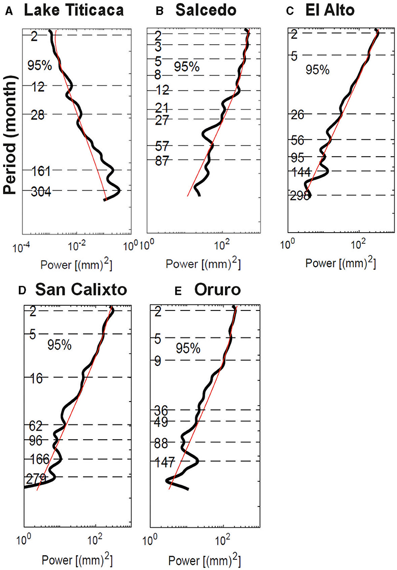
Figure 3. (A) Profile of the global power spectrum of the detrended time series of the monthly anomalies of the water level in Lake Titicaca. (B–E) Profile of the global power spectrum profile of the detrended monthly precipitation for four rain-gauge stations within the Altiplano region (Salcedo, El Alto, San Calixto and Oruro). The horizontal lines represent the peaks of the power spectrum. The dashed line indicates the 95% confidence interval assuming a red noise model suggested by Torrence and Compo (1998). The analysis is based on the 1921–2018 period, except the Salcedo station that only covers the 1930–1990 period.
Figure 3A shows that the power spectrum profile of LTWL presents a semiannual (6 months), annual (12 months), biennial (22–28 months), interannual (80–108 months), decadal (12.75–14.08-year band), interdecadal (25.08 years), and multidecadal (>30 years) signals. The confidence level of the power spectrum profile is based on the red noise model, as suggested by Torrence and Compo (1998). In contrast, Figure 3A indicates that LTWL does not exhibit an intraseasonal component, whereas the precipitation over the Altiplano region displays an intraseasonal component with a roughly 2-month cycle (Figures 3B–E). This latter agrees with the existence of the intraseasonal component of Altiplano precipitation, which was previously documented in Garreaud (2000), Falvey and Garreaud (2005), and Sulca (2023). These results show that oscillations with periods shorter than 3 months do not significantly influence the variability of LTWL.
The existence of the biennial component of LTWL agrees with the biennial component of the monthly precipitation in the Salcedo, El Alto, and San Calixto stations (Figures 3B–D). The existence of the biennial signal is also consistent with previous numeric experiments about the influence of the quasi-biennial oscillation on precipitation over the Central Andes (García-Franco et al., 2022). The interannual band of LTWL agrees with the interannual component of the observed precipitation in the Peruvian and Bolivian Altiplano (Figures 3B–E). In contrast, the interannual band of LTWL does not agree with the significant 6-year band of LTWL in the 1914–2014 period identified in Angulo and Pereira-Filho (2022). The decadal component of LTWL is slightly larger than the decadal band of 12 years and 10–12 years identified in the monthly time series of LTWL in the 1914–2014 and 1914–2016 periods (Alburqueque et al., 2018; Angulo and Pereira-Filho, 2022). The decadal component of LTWL agrees with the decadal component of precipitation in the San Calixto station at 13.83 years, while the remain precipitation stations present a decadal mode that oscillates below 12.75 years (Figures 3B–E). This result is consistent with previous studies about the decadal band of summertime precipitation in the central Andes oscillating between 10 and 13 years (Canedo-Rosso et al., 2019; Sulca et al., 2022a). Due to the decadal band of LTWL is also slightly longer than the decadal band of 10–13 years of summertime precipitation in the central Andes (Sulca et al., 2022a), the precipitation in the central Andes and the LTWL's fluctuations are not necessarily in synchrony in the decadal timescales. The interdecadal band of LTWL is in agreement with the interdecadal band of precipitation in the Peruvian and Bolivian Altiplano above 24 years (Figures 3B–E). This result agrees with previous studies about the interdecadal band of LTWL, which presents significant power bands above 25 years (e.g., Alburqueque et al., 2018).
4 Climatology characteristics of the high- and low-frequency components of LTWL
4.1 Statistical features of LTWL in the high-frequency band
The detrended monthly time series of LTWL and its biennial and interannual components in the 1921–2018 period are shown in Figure 4. Figures 4A, B show that the peaks of the biennial component of the LTWL match better the peaks of the detrended monthly LTWL anomalies than the interannual component of the LTWL. Figure 4B also displays that the interannual component of LTWL does not present a uniform amplitude in the 1921–2018 period. The lowest amplitude of the interannual component of LTWL occurred before 1960 in concordance with the long periods of negative amplitude values in the 80–108-month band (Supplementary Figure S1B). These results show that the biennial component is the leading driver of extreme LTWL episodes in high-frequency timescales.
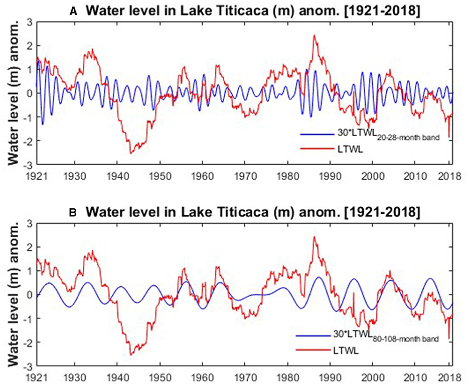
Figure 4. Time series of the detrended monthly anomalies of the water level in Lake Titicaca (m) (original; red line) and its (A) biennial (22–28-month band; blue line) and (B) interannual (80–108-month band; blue line) components. The biennial and interannual components of LTWL were rescaled by a factor of 30. The analysis is based on the 1921–2018 period.
4.2 SST and circulation patterns associated with high-frequency components of LTWL
For the biennial timescale, the biennial component of the LTWL (bLTWL) presents significant southeasterly wind anomalies over the central Andes at 200 hPa (Figure 5A), revealing the humidity flux from the Amazon basin toward the LT basin. The significance analysis of the regressed coefficients is based on the Student-t test at a 95% confidence level (Chatterjee and Hadi, 1986). The upper-level southeasterly wind anomalies are part of the upper-level zonal flow anomalies over South America and the tropical Atlantic Ocean. This indicates the strengthening of the upper-level Bolivian High-Nordeste Low system over South America. In addition, significant northwesterly VIHT anomalies prevail over the eastern flank of the central Andes, indicating a humidity flux coming from the Amazon basin toward Uruguay (e.g., enhanced SALLJ) (Figure 5B). Hence, the mechanism of humidity transport also works for the positive phases of bLTWL.
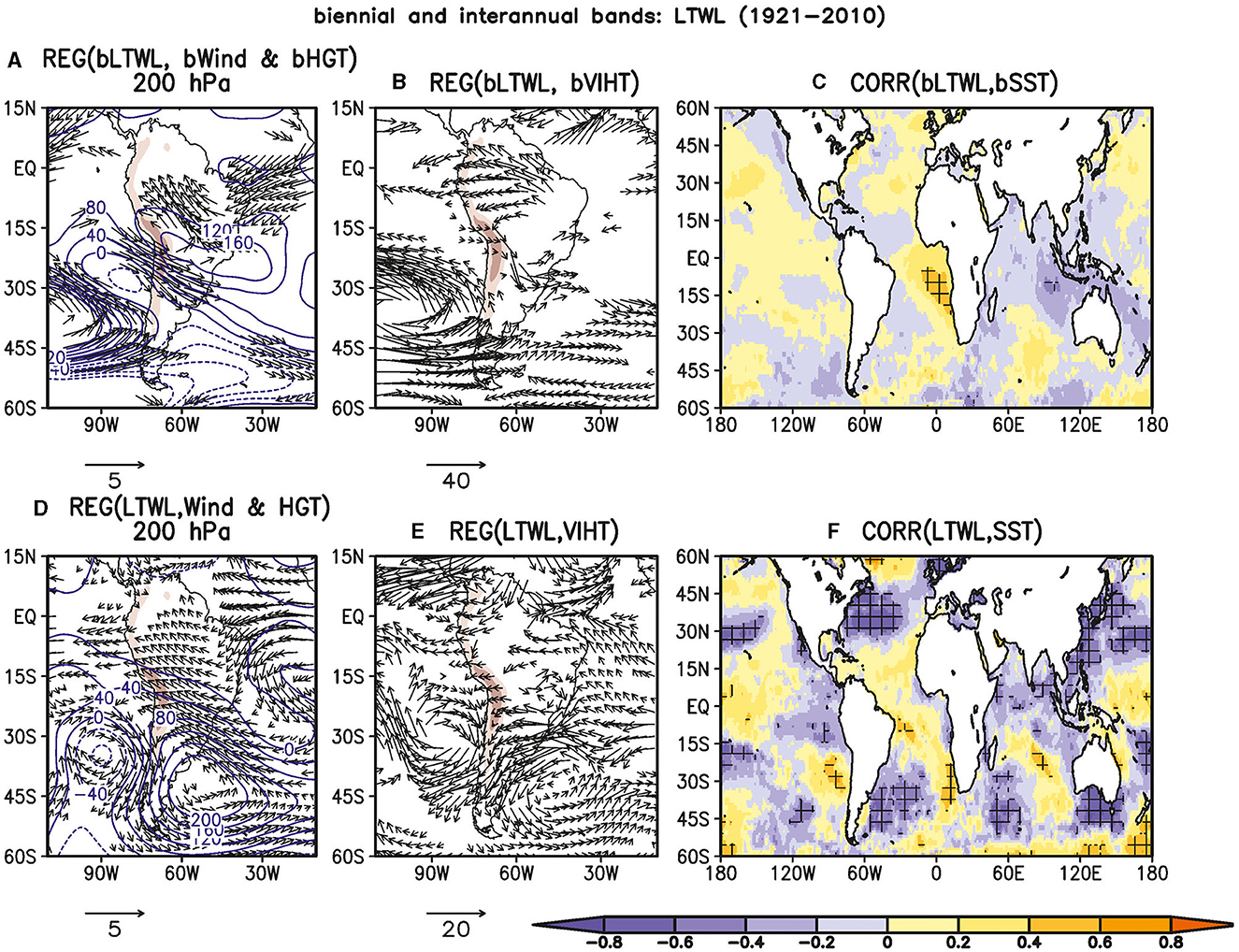
Figure 5. The biennial component of the water level in Lake Tititcaca (bLTWL) regressed upon the biennial component of the (A) 200 hPa wind (bWind, in m s−1 per standard deviation) and geopotential height (bHGT, in m per standard deviation) anomalies and (B) the vertically integrated humidity transport (bVIHT, in kg m−1 s−1 per standard deviation). (C) Correlation coefficients between the monthly time series of the biennial component of the global SST (bSST, °C per standard deviation) anomalies and the monthly time series of the biennial component of the LTWL (D–F). As in (A–C) but for the interannual component of the water level in Lake Tititcaca (LTWL). Black vectors and hatching are statistically significant at the 95% confidence level. The contour interval of geopotential height anomalies is 40 m per standard deviation. The topography above 1,000 m is indicated by brown shading. The ERA-20C reanalysis was used in this analysis. The analysis is for the 1921–2010 period.
Figure 5C shows that bLTWL positively correlates with the biennial component of the SST anomalies over the southeastern tropical Atlantic Ocean. Indeed, Chen et al. (1999) found that the warm SST anomalies over southeastern tropical Atlantic Ocean strengthen the BH-NL system over South America in numeric experiments. Conversely, the bLTWL is not correlated with the biennial component of the SST anomalies over the Pacific and Atlantic Oceans. These results evidence that the change of SST anomalies over southeastern tropical Atlantic Ocean induces the biennial signal of LTWL through the modulation of the intensity of the upper-level BH-NL system.
With respect to interannual timescales, the interannual component of the water level in Lake Titicaca (LTWL) presents significant southeasterly wind anomalies over Peru at 200 hPa (Figure 5D), revealing the humidity flux from the lowland toward the LT basin (Garreaud et al., 2003). The upper-level southeasterly wind anomalies are part of an upper-level anticyclonic circulation located over the southern South Atlantic (51°W, 42°S), indicative of a southeastward displacement of the upper-level Bolivian High. In addition, significant easterly VIHT anomalies prevail over the central Andes, indicating a humidity flux coming from the northern South Atlantic (Figure 5E). This agrees with the humidity mechanism associated with the summertime wet episodes over the Altiplano region (Garreaud, 1999; Vuille, 1999; Segura et al., 2019). Hence, the mechanism of humidity transport also works for the positive phases of the interannual component of the LTWL.
Figure 5F shows that LTWL positively correlates with the interannual component of the SST anomalies over the tropical South Atlantic and negatively correlates with southern South Atlantic, northwestern North Atlantic and western North Pacific. In addition, Figure 6 shows that the southern South Atlantic is the unique SST index with a quasi-uniform average lag of 3 months with the time series of the interannual component of the LTWL. These results evidence that the change of SST anomalies over the southern South Atlantic is the main modulator of the interannual component of the LTWL.
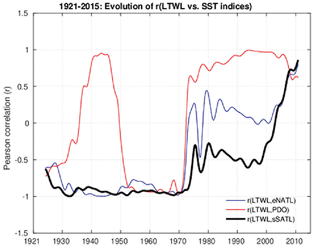
Figure 6. Evolution of the Pearson correlation between the time series of the interannual component of the water level in Lake Titicaca (LTWL) and the monthly time series of the interannual component of the SST anomalies in the extratropical North Atlantic Ocean (eNATL, blue line), the Pacific Decadal Oscillation (PDO, red line) and southern South Atlantic Ocean (sSATL, bold black line). The Pearson correlation is based on 101 consecutive months in the interannual timescales (80–108-month band). The analysis is based on the 1921–2015 period.
On the other hand, the SST anomalies in the central and eastern Pacific Ocean do not present significant correlations with the interannual component of the LTWL, indicating that the change of the SST anomalies in the equatorial Pacific do not drive the interannual component of the LTWL alone.
4.3 SST and circulation patterns associated with low-frequency components of LTWL
On a decadal timescale, the decadal component of the LTWL (dLTWL) presents significant northeasterly wind anomalies over the central Andes at 200 hPa (Figure 7A), revealing the enhancement of the humidity flux from the Amazonia toward the LT basin. Significant northeasterly VIHT anomalies prevail along the eastern flank of the central Andes (Figure 7B), indicative of an enhanced SALLJ on decadal timescales. These northeasterly VIHT anomalies from the Tropical North Atlantic reveal that the humidity transport mechanism also drives positive LTWL phases on the decadal timescale.
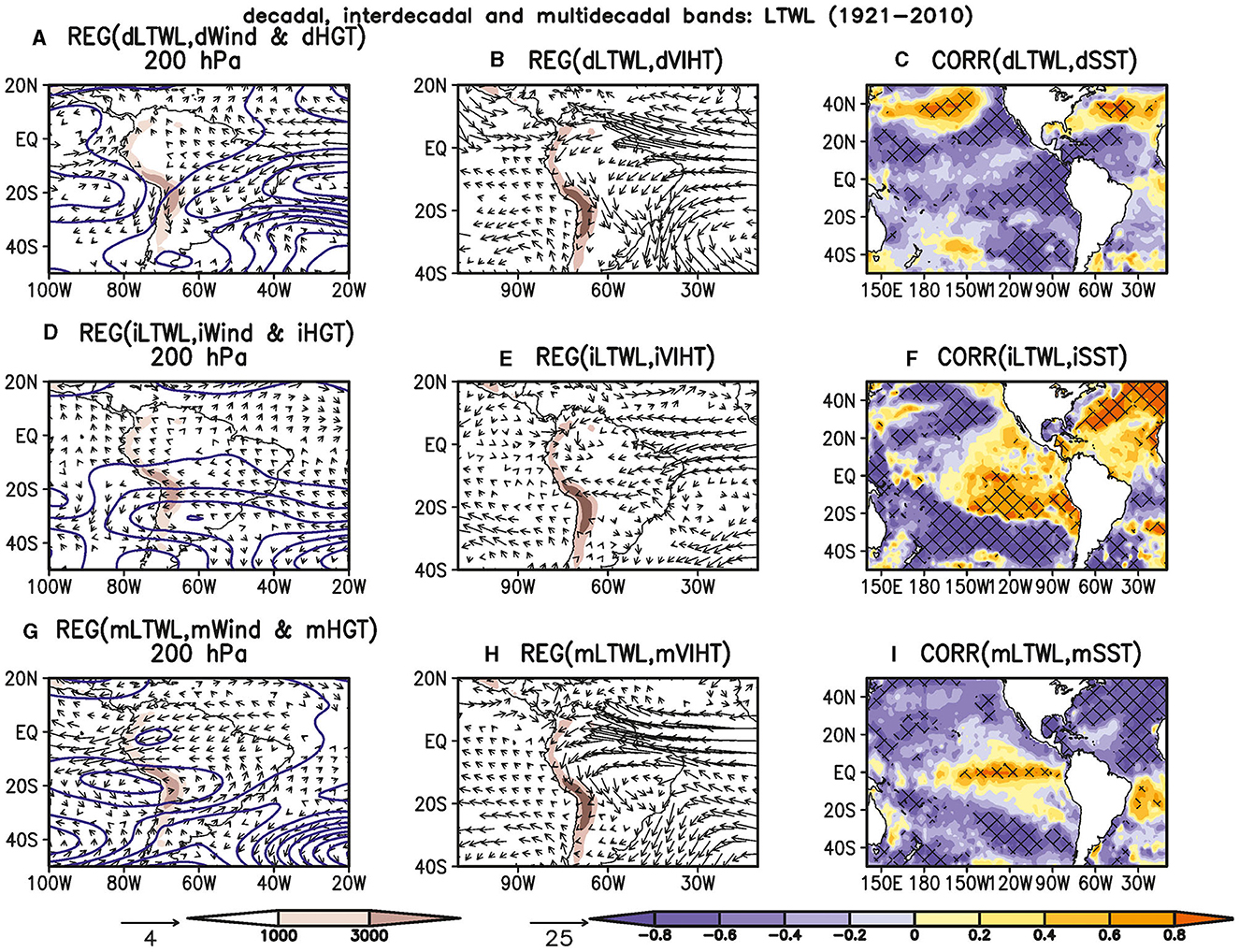
Figure 7. The decadal component of the water level in Lake Tititcaca (dLTWL) regressed upon the decadal component of the (A) 200 hPa wind (dWind, in m s−1 per standard deviation) and geopotential height (dHGT, in m per standard deviation) anomalies and (B) the vertically integrated humidity transport (dVIHT, in kg m−1 s−1 per standard deviation). (C) Correlation coefficients between the monthly time series of the decadal component of the global SST (dSST, °C per standard deviation) anomalies and the monthly time series of the decadal component of the LTWL (dLTWL, m per standard deviation). (D–F) As in (A–C) but for the interdecadal component of the water level in Lake Tititcaca (iLTWL). (G–I) As in (A–C) but for the multidecadal component of the water level in Lake Tititcaca (mLTWL). Black vectors and hatching are statistically significant at the 95% confidence level. The contour interval of geopotential height anomalies is 200 m per standard deviation. The topography above 1,000 m is indicated by brown shading. The ERA-20C reanalysis was used in this analysis. The analysis is for the 1921–2010 period.
The dLTWL index negatively correlates with the decadal component of the SST anomalies over the Pacific basin (dE, dN1 +2, and dN3) and tropical North Atlantic (dtNATL) (Figure 7C). The significance analysis of the correlation SST pattern is based on the Student-t test, which accounts for the autocorrelation using the effective degrees of freedom at a 95% confidence level (Davis, 1976; Zhao and Khalil, 1993). Figure 7C also shows an dSST dipole over the North Pacific north of 20°N, but it does not resemble the PDO SST pattern (Mantua et al., 1997). In addition, Supplementary Table S1 shows the negative correlations between the dLTWL and dE, dN1 + 2, dN3, and dPDO indices (r < −0.5, p < 0.05). Supplementary Table S1 also shows that the negative correlation related to the dPDO is weaker than those of the dE and dN1 + 2, revealing that the dSST anomalies in the eastern equatorial Pacific correlate better with the dLTWL than the North Pacific dSST anomalies. The negative correlation between dLTWL and dtNATL is consistent with the reduction in precipitation over the southeastern Bolivian Altiplano during the warm phase of the decadal component (8–16-year band) of the AMO, which weakens the humidity flux from the Amazon basin to the southeastern Bolivian Altiplano (Canedo-Rosso et al., 2019).
For the interdecadal timescale, the interdecadal component of the LTWL (iLTWL) present significant easterly wind anomalies over the central Andes at 200 hPa, revealing the humidity flux from the subtropical lowland toward the LT basin (Figure 7D). The upper-level easterly wind anomalies are part of an anticyclonic circulation anomaly over the Chilean Andes, indicating the southward shift of the Bolivian High. In addition, significant easterly VIHT anomalies prevail over the eastern flank of Southern Bolivia toward the central Andes, indicating a humidity flux coming from the northern South Atlantic (Figure 7E). Hence, the mechanism of humidity transport also works for the positive phases of iLTWL as in the interannual timescales.
Figure 7F shows that iLTWL positively correlates with the interdecadal component of the SST anomalies over the extratropical North Atlantic, the central Pacific, and the coasts of Peru and northern Chile. Conversely, the iLTWL has a negative linear relationship with the interdecadal component of the SST anomalies over the tropical and southern parts of the South Atlantic Ocean.
Regarding the multidecadal timescale, the multidecadal component of the LTWL (mLTWL) features significant easterly wind anomalies over the central Andes at 200 hPa (Figure 7G), revealing a strengthening of the humidity flux from the subtropical lowland toward the LT basin. The upper-level easterly wind anomalies are part of an anticyclonic circulation anomaly located in front of southern Peru-northern Chile's coasts, indicating the westward displacement of the Bolivian High. Furthermore, the upper-level wind anomalies agree with significant northeasterly VIHT anomalies over the eastern flank of the Peruvian Andes (Figure 7H), indicating a humidity flux coming from the tropical North Atlantic (Jones and Carvalho, 2019). Hence, the mechanism of humidity transport also works for the multidecadal component of the LTWL.
Figure 7I shows that mLTWL positively correlates with the multidecadal component of the SST anomalies over the central and eastern Pacific (mE and mC) and tropical South Atlantic (mtSATL). The mLTWL index has a negative relationship with the entire North Atlantic and a dipole mSST anomaly over the southern South Atlantic.
5 Multiple linear regression models
On a decadal timescale, Figure 8A shows that the MLR1 model reproduces the decadal component of LTWL (dLTWL). Indeed, the observed and estimated time series of the LTWL have a significant correlation (r = 0.95, p < 0.05; Table 2). Thus, the linear combination of the decadal component of the SST anomalies in the central and eastern Pacific (dC and dE), extratropical North Atlantic (deNATL), and southern South Atlantic (dsSATL) explains dLTWL. The dE presents the highest correlation with dLTWL (Supplementary Table S1). This result also shows that the decadal component of the LTWL is more closely associated with the decadal component of the SST anomalies over the central and eastern equatorial Pacific (dC and dE) than in the northern Pacific (dPDO). It agrees with the weaker negative correlation between dLTWL and the dPDO with respect to the negative correlation between dLTWL and the dE and dN1+2 indices (Supplementary Table S1). When the deNATL predictor is not considered in the MLR1 model, the correlation between the observed and estimated time series of LTWL weakens to 0.71. It reveals the key role of the deNATL index on the decadal variability of the LTWL. Indeed, numeric experiments suggested upper-level easterly wind anomalies over South America at 200 hPa in response to warm SST anomalies over the North Atlantic on the decadal timescale (An et al., 2021).
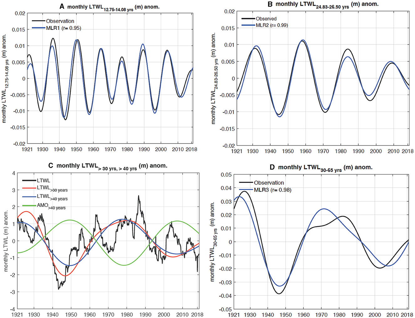
Figure 8. (A) Monthly time series of the observations (blue line) and MLR1 model reconstructions (red line) for the decadal component in the 12.75–14.08-year band of the monthly time series of the water level in Lake Titicaca (m). (B) Same as (A) but for the interdecadal component of the monthly time series of the LTWL in the 24.83–26.50-year band. (C) Monthly time series of the LTWL (black line) and the low-frequency components of the 30-year (red line) and 40-year (blue line) bands. The green line represents the filtered monthly time series of the LTWL for the multidecadal bands of more than 40 years. (D) Same as (A) but for the multidecadal component of the monthly time series of the LTWL in the 30–65-year band. The analysis is based on the 1921–2018 period.
Table 2. Intercept and coefficient of the predictors of the multiple linear regression (MLR) models for the decadal, interdecadal, and multidecadal components of the monthly time series of the LTWL based on the decadal (12.75–14.08-year band), interdecadal (24.83–26.50-year band), and multidecadal (30–65-year band) components of the Pacific and Atlantic SST indices and the AMO index in the 1921–2018 period.
Regarding the interdecadal timescale, MLR2 reproduces the interdecadal component of the LTWL (r = 0.99, p < 0.05; Table 2) (Figure 8B). Thus, the linear combination of the interdecadal component of the SST anomalies over the far-eastern Pacific (iN1 + 2), southern South Atlantic Ocean (isSATL), and SST anomalies in the central and eastern Pacific (iC and iE), extratropical North Atlantic (ieNATL), and southern South Atlantic (isSATL) indices explains iLTWL. In addition, the ieNATL index is better correlated with the iLTWL than the iAMO (r = 0.93, p < 0.05) (Supplementary Table S2). When we repeat the same experiment using the Pacific SST indices solely, the MLR2 model cannot reproduce the observed profile of the interdecadal component of LTWL (e.g., iLTWL). These results reveal that the interdecadal component of Pacific SST anomalies does not drive iLTWL alone.
For the multidecadal timescale, we apply the filter low-pass analysis for oscillations of more than 30 years (LTWL>30years). Figure 8C displays that the multidecadal components of more than 30 and 40 years of the AMO index is concordant with the profile of LTWL>30years. Indeed, the AMO index and LTWL>30years are positively correlated (r > 0.98, p < 0.05; Table 2). However, the profile of LTWL>30years cannot duplicate the observed profile of the LTWL, suggesting that the superposition of the interdecadal and multidecadal components of LTWL creates the original profile of LTWL. We restrict the multidecadal signal in the 30–65-year band to test this hypothesis. Figure 8D shows that the MLR model works well for the multidecadal band of 30–65 years of the LTWL (r = 0.98, p < 0.05; Table 2). These results highlight that the multidecadal band of 30–65 years of the LTWL can be described as the linear combination of the multidecadal band of 30–65 years of the SST anomalies in the southern South Atlantic (msSATL) and the AMO (mAMO) indices. The negative regressed coefficient of the mAMO agrees with the significant negative correlation between the mLTWL and the multidecadal component of the SST anomalies over the entire North Atlantic (r > −0.65, p < 0.05; Supplementary Table S3). These results agree with the dynamic link between austral summer precipitation over the central Andes and southern Atlantic SST anomalies on long timescales (>30 years) (Sulca et al., 2022b).
6 Trend analysis for LTWL
The results of the breakpoint analysis for the time series of non-detrended monthly anomalies of LTWL and their respective trends from 1921 to 2018 are presented in Figure 9. In Figure 9A, it can be observed that the LTWL time series exhibits four breakpoints in February 1940, February 1949, March 1974, and April 1990. Figure 9B shows that the first period (January 1921–February 1940) presents a negative trend of −0.0036 m month−1. The second period, spanning from March 1940 to February 1949, exhibits a positive trend of 0.0021 m month−1 (Figure 9C). Figures 9D, E display that the third and fourth periods (March 1949–March 1979 and April 1974–April 1990) also present a positive trend of 0.0014 and 0.0043 m month−1. Conversely, the fifth period (May 1990 to December 2018) shows a trend equal to zero. According to Figure 9, the value of the tendency of LTWL in the first four periods follows the change of phase of the multidecadal components of LTWL, whereas the lack of a trend in LTWL in the fifth period is caused by the reduction of the amplitude of the interdecadal component of LTWL since the 1990s (Figure 8D). When we repeat the same analysis for the entire period (1921–2018), water level in Lake Titicaca presents a positive trend of 0.0005 m month−1, which is an order of magnitude lower compared to the five epochs.
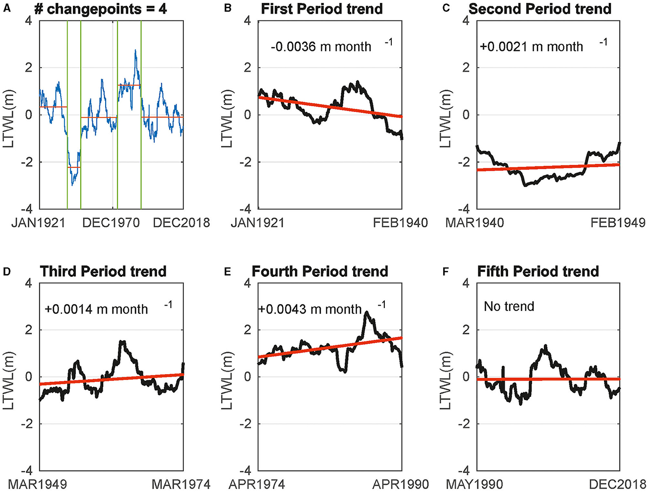
Figure 9. (A) The number of the change points of the monthly time series of the water level in Lake Titicaca. Trend analysis for the five epochs within the 1921–2018 period: (B) first period (January 1921–February 1940), (C) second period (March 1940–February 1949), (D) third period (March 1949–March 1974), (E) fourth period (April 1974–April 1990), and (F) fifth period (May 1990–December 2018). (A) # changepoints = 4. (B) First Period trend. (C) Second Period trend. (D) Third Period trend. (E) Fourth Period trend. (F) Fifth Period trend.
7 Summary and conclusions
Understanding the biennial, decadal, and multidecadal variability of the water level fluctuation in Lake Titicaca is useful for developing prediction models covering seasonal to multidecadal timescales. These tools will provide useful information to water management in the face of major changes in hydrological behavior in the Lake Titicaca basin. Characterize the biennial (22–28-month band), interannual (80–108-month band) and longtime (>10 years) components of the water level in Lake Titicaca based on continuous wavelet techniques, high and low band filter, and composite analysis, reveal features of the hydroclimate regime that have not been explored and need further investigation to constrain the water management tools better.
The oscillations with periods shorter than 3 months do not significantly influence the variability of LTWL on high-frequency timescales. In contrast, the high-frequency variability of the LTWL is governed by its biennial (22–28-month band) and interannual (80–108-month band) components. The biennial signal is the leading component of the high-frequency component of LTWL because it agrees better with the most extreme episodes of LTWL than the interannual component. Dynamically, the biennial component of the LTWL is induced by the change of SST anomalies over southeastern tropical Atlantic Ocean that enhances humidity flux transport from the Amazon basin through the strengthening of the upper-level BH-NL system over South America (Chen et al., 1999).
On interannual timescales, the mechanism of humidity transport from northern South Atlantic toward the Altiplano region drives interannual component of the LTWL. This transport mechanism is caused by the southerly easterly wind anomalies over the Altiplano region by the southeastward displacement of the upper-level Bolivian High over the southern South Atlantic Ocean (51°W, 42°S). Thus, change of the SST anomalies over southern South Atlantic Ocean is the main modulator of the interannual component of the LTWL because LTWL and sSATL have a significant and persistent negative correlation in the 1921–2018 period. The change of sign of this linear correlation would be associated with the apparition of the atmospheric teleconnection between the precipitation in the central Andes with the deep convection over the northwestern Amazon basin since 2000s (Segura et al., 2020).
The mechanism of humidity transport drives all low-frequency components of the LTWL, but their low- and upper-level atmospheric circulation forcings are different. At low levels, the enhanced SALLJ drives the decadal and multidecadal components of the LTWL (Figures 7B, H). In contrast, the easterly humidity flux coming from the northern South Atlantic toward the Lake Titicaca basin drives the interdecadal component of LTWL (Figure 7E). It is caused by the remote effect of the SST anomalies over the southern South Atlantic on the position of the Bolivian High (Figure 7F). In the upper troposphere, the change of position of the Bolivian High is relevant to driving interdecadal and multidecadal components of the LTWL (Figures 7D, G).
The low-frequency components of the LTWL can be described as the overlap of the long-term variability of the Pacific and Atlantic SST anomalies. For instance, the decadal component of the LTWL is explained as the overlap of the decadal component of the ENSO Pacific (dE and dC), extratropical North Atlantic (deNATL) and southern South Atlantic (dsSATL) indices. In addition, the PDO alone cannot drive the decadal component of the LTWL. The interdecadal component of the LTWL can be explained by the linear combination of the interdecadal component of the Niño 1 + 2 (iN1+2), extratropical North Atlantic (ieNATL), and southern South Atlantic (isSATL) indices. The multidecadal component of the LTWL in the 30–65-year band is explained by the overlap of the multidecadal component in the 30–65-year band of the southern and northern parts of the South Atlantic Ocean and the AMO index. Moreover, the multidecadal component of the southern South Atlantic SST anomalies explains the multidecadal variability in the LTWL before 1960.
The trends of the water level in Lake Titicaca from January 1921 to April 1990 were caused by the multidecadal components of LTWL. The weakening of the interdecadal component of the LTWL explained a trend equal to zero of LTWL from May 1990 to December 2018.
The climate modes of the SST anomalies over the Pacific basin (Niño1 + 2, Niño 4, and PDO) can cause extreme water levels of Lake Titicaca. However, they cannot drive Lake Titicaca's water level low-frequency variability alone.
Finally, additional analysis is required to develop a prediction model and understand future LTWL changes. In the context of developing the prediction model, it is important first to characterize the extreme fluctuations of LTWL to identify the primary predictors necessary for building statistical prediction models. This is because the time series of LTWL and precipitation in the Altiplano region exhibit different high-frequency components and distinct large-scale atmospheric circulation patterns (Sulca et al., 2022a,b). Regarding the future projection of LTWL, it is necessary to analyze the future projections of ENSO, PDO, and AMO in CMIP5 and CMIP6 models. These can be used as predictors to forecast changes in the interannual, interdecadal, and multidecadal components of Lake Titicaca's water level and their potential impacts on extreme LTWL events by the end of the 21st century.
8 Scope statement
The Lake Titicaca basin (LTB) is located in the Altiplano region between Peru and Bolivia at 68°33'-70°1'W and 15°6'-16°50'S with an average altitude of 3810 m asl. The LT basin contains several large paramos of Peru and Bolivia. The water supply of LT is important for local ecosystems and various economic activities, such as industry, fishing, agriculture, and tourism. However, several studies have projected a great reduction in precipitation over the Central Andes between the middle and the end of the 21st century. Hence, the volume of water in LT will become the main source of water for the population, all species, and ecosystems in the LT basin in the coming decades due to climate change. For these reasons, we want to submit the manuscript entitled “New insights into the biennial-to-multidecadal variability of the water level fluctuation in Lake Titicaca in the 20th Century,” which describes the influence of the Pacific, Atlantic, and southeastern tropical Atlantic Ocean SST anomalies on the high- and low-frequency modes of the water level in Late Titicaca. The outcomes will help to improve and create water management policies and forecasting systems for the LWLT and, thus, reduce the impact of climate change in the LTB.
Data availability statement
The original contributions presented in the study are included in the article/Supplementary material, further inquiries can be directed to the corresponding author/s.
Author contributions
JS: Conceptualization, Data curation, Formal analysis, Methodology, Software, Validation, Visualization, Writing – original draft, Revised draft. JA: Formal analysis, Funding acquisition, Investigation, Methodology, Validation, Visualization, Writing – original draft, Revised draft. JT: Formal analysis, Investigation, Methodology, Validation, Visualization, Writing – original draft, Revised draft.
Funding
The author(s) declare financial support was received for the research, authorship, and/or publication of this article. PROCIENCIA partially supported JA in reference to contract N °124−2020 FONDECYT, Perú. The work was performed using computational resources, HPC-Linux-Cluster, from Laboratorio de Dinámica de Fluidos Geofísicos Computacionales at Instituto Geofísico del Perú (grants 101–2014-FONDECYT).
Acknowledgments
The authors would like to express their gratitude to Ing. Sixto Flores for generously providing the monthly time series data of Lake Titicaca's water levels. We are also grateful to SENAMHI (Servicio Nacional de Meteorología e Hidrología) in Peru and its counterpart in Bolivia for supplying us with the precipitation data. The authors extend their appreciation to Dr. Yamina Silva for her valuable initial comments and feedback. The authors express their gratitude to the two reviewers who played a crucial role in enhancing the quality of this manuscript's results.
Conflict of interest
The authors declare that the research was conducted in the absence of any commercial or financial relationships that could be construed as a potential conflict of interest.
Publisher's note
All claims expressed in this article are solely those of the authors and do not necessarily represent those of their affiliated organizations, or those of the publisher, the editors and the reviewers. Any product that may be evaluated in this article, or claim that may be made by its manufacturer, is not guaranteed or endorsed by the publisher.
Supplementary material
The Supplementary Material for this article can be found online at: https://www.frontiersin.org/articles/10.3389/fclim.2023.1325224/full#supplementary-material
References
Alburqueque, E., Espino, M., Segura, M., and Chura, R. (2018). Nivel hídrico y precipitaciones del lago Titicaca en relación con las variables de macroescala del océano Pacífico. Trad. Segunda época. 17, 36–43. doi: 10.31381/tradicion.v0i17.1364
Alvarez, M. S., Vera, C. S., Kiladis, G. N., and Liebmann, B. (2016). Influence of the Madden-Julian Oscillation on South America's precipitation and surface air temperature. Clim. Dyn. 46, 245–262. doi: 10.1007/s00382-015-2581-6
An, X., Wu, B., Zhou, T., and Liu, B. (2021). Atlantic multidecadal oscillation drives interdecadal Pacific variability via tropical atmosphere bridge. J. Clim. 34, 5543–5553. doi: 10.1175/JCLI-D-20-0983.1
Angulo, E. C., and Pereira-Filho, A. J. (2022). Ocean forcing on Titicaca Lake water volume. Open J. Mod. Hydrol. 12, 1–10. doi: 10.4236/ojmh.2022.121001
Angulo, E. C., and Pereira-Filho, A. J. (2023). Extreme droughts and their relationship with the Interdecadal Pacific Oscillation in the Peruvian Altiplano region over the last 100 years. Atmosphere. 14, 1233. doi: 10.3390/atmos14081233
Beaton, R. H., and Tukey, J. W. (1974). The fitting of power series, meaning polynomials, illustrated on band-spectroscopic data. Technometrics 16, 147–185. doi: 10.1080/00401706.1974.10489171
Canedo, C., Pillco-Zol,á, R., and Berndtsson, R. (2016). Role of hydrological studies for the development of the TDPS system. Water. 8, 144. doi: 10.3390/w8040144
Canedo-Rosso, C., Uvo, C. B., and Berndtsson, R. (2019). Precipitation variability and its relation to climate anomalies in the Bolivian Altiplano. Int. J. Climatol. 39, 2096–2107. doi: 10.1002/joc.5937
Centro de Ciencia del Clima y la Resilencia (CR)2 (2018). Simulaciones Climáticas Regionales y marco de Evaluación de la Vulnerabilidad. Ministerio del Medio Ambiente de Chile. Available online at: www.cr2.cl (accessed April 1, 2021).
Chatterjee, S., and Hadi, A. S. (1986). Influential observations, high leverage points, and outliers in linear regression. Stat. Sci. 1, 379–416. doi: 10.1214/ss/1177013622
Chen, T.-S., Weng, S.-P., and Schubert, S. (1999). Maintenance of austral summertime upper-tropospheric circulation over tropical South America: the bolivian high-nordeste low system. J. Atm. Sci. 56, 2081–2100. doi: 10.1175/1520-0469(1999)056<2081:MOASUT>2.0.CO;2
Chura-Cruz, R., Cubillos, L. A., Tam, J., Segura, M., and Villanueva, C. (2013). Relationship between lake water level and rainfall on the landing of Argentinian Silverside Odontesthes bonariensis (Valenciennes, 1835) in the Peruvian sector of the Titicaca Lake from 1981 to 2010. Ecol. Aplic. 12, 19–28. doi: 10.21704/rea.v12i1-2.434
Dai, A. (2013). The influence of the inter-decadal Pacific oscillation on US precipitation during 1923-2010. Clim. Dyn. 41, 633–646. doi: 10.1007/s00382-012-1446-5
Davis, R. E. (1976). Predictability of sea surface temperature and sea level pressure anomalies over the North Pacific Ocean. J. Phys. Oceanogr. 6, 249–266. doi: 10.1175/1520-0485(1976)006<0249:POSSTA>2.0.CO;2
Deser, C., Phillips, A. S., and Hurrell, J. W. (2004). Pacific interdecadal climate variability: linkages between the tropics and the North Pacific during boreal winter since 1900. J. Clim. 17, 3109–3124. doi: 10.1175/1520-0442(2004)017<3109:PICVLB>2.0.CO
Dong, B., and Dai, A. (2016). The influence of the Interdecadal Pacific Oscillation on temperature and precipitation over the globe. Clim. Dyn. 45, 2667–2681. doi: 10.1007/s00382-015-2500-x
DuMouchel, W. H., and O'Brien, F. L. (1989). “Integrating a robust option into a multiple regression computing environment,” in Computer Science and Statistics/Proc. 21st Symposium On the Interface (Alexandria, VA, American Statistical Association) 297–302.
Enfield, D. B., Mestas-Nuñez, A. M., and Trimble, P. (2001). The Atlantic multidecadal oscillation and its relation to rainfall and river flows in the continental U.S. Geophys. Res. Lett. 28, 2077–2080. doi: 10.1029/2000GL012745
Falvey, M., and Garreaud, R. D. (2005). Moisture variability over the South American Altiplano during the South American Low-Level Jet Experiment (SALLJEX) observing season. J. Geophys. Res. 110, D22105. doi: 10.1029/2005JD006152
Fernandes, L. G., and Grimm, A. M. (2023). ENSO modulation of the global MJO and its impacts on South America. J. Clim. 36, 7715–7738. doi: 10.1175/JCLI-D-22-0781.1
García-Franco, J. L., Gray, L. J., Osprey, S., Chadwick, R., and Martin, Z. (2022). The tropical route of quasi-biennial oscillation (QBO) teleconnections in a climate model Weather. Clim. Dyn. 3, 825–844. doi: 10.5194/wcd-3-825-2022
Garreaud, R., Vuille, M., and Clement, A. C. (2003). The climate of the Altiplano: observed current conditions and mechanisms of past changes. paleogeogr. Palaeoclimatol. Paleoecol. 194, 5–22. doi: 10.1016/S0031-0182(03)00269-4
Garreaud, R. D. (1999). Multiscale analysis of the summertime precipitation over the central Andes. Mon. Whe. Rev. 127, 901–921. doi: 10.1175/1520-0493(1999)127<0901:MAOTSP>2.0.CO;2
Garreaud, R. D. (2000). Intraseasonal variability of moisture and rainfall over the South American Altiplano. Mon. Wea. Rev. 128, 3337–3346. doi: 10.1175/1520-0493(2000)128<3337:IVOMAR>2.0.CO;2
Garreaud, R. D., and Aceituno, P. (2001). Interannual rainfall variability over the South American Altiplano. J. Clim. 14, 2779–2789. doi: 10.1175/1520-0442(2001)014<2779:IRVOTS>2.0.CO;2
Grimm, A. M. (2019). “South American monsoon and its extremes,” in Tropical Extremes: Natural Variability and Trends, eds V. J. Vuruputur et al. (Elsevier), 51–93. doi: 10.1016/B978-0-12-809248-4.00003-0
Grinsted, A., Moore, J. C., and Jevrejeva, S. (2004). Application of the cross wavelet transform and wavelet coherence to geophysical time series. Nonlinear Process. Geophys. 11, 561–566. doi: 10.5194/npg-11-561-2004
Hao, Z., Singh, V. P., and Hao, F. (2018). Compound extreme in hydroclimatology: review. Water. 10, 718. doi: 10.3390/w10060718
Hastenrath, S., and Kutzbach, J. (1985). Late Pleistocene climate and water budget of the South American Altiplano. Quat. Res. 24, 249–256. doi: 10.1016/0033-5894(85)90048-1
He, Z., Dai, A., and Vuille, M. (2021). The joint impacts of Atlantic and Pacific multidecadal variability on South American precipitation and temperature. J. Clim. 34, 1–55. doi: 10.1175/JCLI-D-21-0081.1
Huang, H., Winter, J. M., Osterberg, E. C., Horton, R. M., and Beckage, B. (2017). Total and extreme precipitation changes over the Northeastern United States. J. Hydrometeo. 18, 1783–1798. doi: 10.1175/JHM-D-16-0195.1
Imfeld, N., Barreto-Schuler, C., Correa-Marrou, K. M., Jacques-Coper, M., Sedlmeier, K., and Gubler, S. (2019). Summertime precipitation deficits in the southern Peruvian highlands since 1964. Int. J. Climatol. 39, 4497–4513. doi: 10.1002/joc.6087
Jones, J. (2019). Recent changes in the South America low-level jet. NPJ Clim. Atmos. Sci. 2, 20. doi: 10.1038/s41612-019-0077-5
Jones, J., and Carvalho, L. M. V. (2019). The influence of the Atlantic multidecadal oscillation on the eastern Andes low-level jet and precipitation in South America. NPJ Clim. Atmos. Sci. 1, 40. doi: 10.1038/s41612-018-0050-8
Killick, R., Fearnhead, P., and Eckley, I. A. (2012). Optimal detection of changepoints with a linear computational cost. J. Am. Stat. Assoc. 107, 1590–1598. doi: 10.1080/01621459.2012.737745
Knight, J. R., Folland, C. K., and Scaife, A. A. (2006). Climate impacts of the Atlantic multidecadal oscillation. Geophys. Res. Lett. 33, L17706. doi: 10.1029/2006GL026242
Kodama, Y. (1992). Large-scale common features of subtropical precipitation zones (the baiu frontal zone, the SPCZ and the SACZ) Part I: characteristics of subtropical frontal zones. J. Meteor. Soc. Jpn. 70, 813–836. doi: 10.2151/jmsj1965.70.4_813
Labat, D., Espinoza, J. C., Ronchail, J., Cochonneau, G., de Oliveira, E., Doudou, J. C., et al. (2012). Fluctuations in the monthly discharge of Guyana shield rivers, related to Pacific and Atlantic climate variability. Hydrol. Sci. 57, 1–11. doi: 10.1080/02626667.2012.695074
Labat, D., Ronchail, J., and Guyot, J. L. (2005). Recent advances in wavelet analyses: Part 2—Amazon, Parana, Orinoco and Congo discharges time scale variability. J. Hydrol. 314, 289–311. doi: 10.1016/j.jhydrol.2005.04.004
Lavado-Casimiro, W., and Espinoza, J. C. (2014). Impact of El Niño and La Niña on rainfall in Peru. Rev. Bras. Meteorol. 29, 171–182. doi: 10.1590/S0102-77862014000200003
Lenters, J. D., and Cook, K. H. (1995). Simulation and diagnosis of the regional summertime precipitation climatology of South America. J. Clim. 8, 2988–3005. doi: 10.1175/1520-0442(1995)008<2988:SADOTR>2.0.CO;2
Lenters, J. D., and Cook, K. H. (1997). On the origin of the Bolivian high and related circulation features of the South American climate. J. Atmos. Sci. 54, 656–678. doi: 10.1175/1520-0469(1997)054<0656:OTOOTB>2.0.CO;2
Liebmann, B., Kiladis, G. N., Marengo, J. A., Ambrizzi, T., and Glick, J. D. (1999). Submonthly convective variability over South America and the South Atlantic convergence zone. J. Clim. 12, 1877–1891. doi: 10.1175/1520-0442(1999)012<1877:SCVOSA>2.0.CO;2
Lima-Quispe, N., Escobar, M., Wickel, A. J., von Kaenel, M., and Purkey, D. (2021). Untangling the effects of climate variability and irrigation management on water levels in Lakes Titicaca and Poopó. J. Hydrol. Reg. Stud. 37, 100927. doi: 10.1016/j.ejrh.2021.100927
Liu, Y., Liang, X. S., and Weisberg, R. H. (2007). Rectification of the bias in the wavelet power spectrum. J. Atmos. Ocean. Technol. 24, 2093–2102. doi: 10.1175/2007JTECHO511.1
Madden, R. A., and Julian, P. R. (1972). Description of global-scale circulation cells in the tropics with a 40-50-day period. J. Atmosph. Sci. 29, 1109–1123. doi: 10.1175/1520-0469(1972)029<1109:DOGSCC>2.0.CO;2
Madden, R. A., and Julian, P. R. (1994). Observations of the 40- 50-day tropical oscillation: a review. Monthly Weather Rev. 122, 814–837. doi: 10.1175/1520-0493(1994)122<0814:OOTDTO>2.0.CO;2
Mantua, N. J., Hare, S. R., Zhang, Y., Wallace, J. M., and Francis, R. C. (1997). A Pacific interdecadal climate oscillation with impacts on salmon production. Bull. Am. Meteorol. Soc. 78, 1069–1080. doi: 10.1175/1520-0477(1997)078<1069:APICOW>2.0.CO;2
Mayta, V. C., Ambrizzi, T., Espinoza, J. C., and Silva Días, P. L. (2019). The role of the Madden-Julian oscillation on the Amazon Basin intraseasonal rainfall variability. Int. J. Climatol. 39, 343–360. doi: 10.1002/joc.5810
McPhaden, M. J., Zebiak, S. E., and Glantz, S. E. (2006). ENSO as an integrating concept in Earth science. Science. 314, 1740–1745. doi: 10.1126/science.1132588
Ministerio del Ambiente (2013). Línea de base Ambiental de la cuenca del Lago Titicaca. Ministerio del Ambiente. 79. Available online at: https://sinia.minam.gob.pe/sites/default/files/sinia/archivos/public/docs/4170.pdf (accessed June 20, 2023).
Minvielle, M., and Garreaud, R. D. (2011). Projecting rainfall changes over the South American Altiplano. J. Clim. 24, 4577–4583. doi: 10.1175/JCLI-D-11-00051.1
Montini, T. L., Jones, C., and Carvalho, L. M. V. (2019). The South American low-level jet: a new climatology, variability, and changes. J. Geophys. Res. Atmos. 124, 1200–1218. doi: 10.1029/2018JD029634
Morales, J. S., Crispín-DelaCruz, D. B., Álvarez, C., Christie, D. A., Ferrero, M. E., Andreu-Hayles, L., et al. (2023). Drought increase since the mid-20th century in the northern South American Altiplano revealed by a 389-year precipitation record. Clim. Past. 19, 457–476. doi: 10.5194/cp-19-457-2023
Neukom, R., Rohrer, M., Calanca, P., Salzmann, N., Huggel, C., Acuña, D., et al. (2015). Facing unprecedented drying of the Central Andes? Precipitation variability over the period AD 1000-2100. Environ. Res. Lett. 10, 084017. doi: 10.1088/1748-9326/10/8/084017
Poli, P., Hersbach, H., Dee, D. P., Berrisford, P., Simmons, A. J., Vitart, F., et al. (2016). ERA-20C: an atmospheric reanalysis of the twentieth century. J. Clim. 29, 4083–4097. doi: 10.1175/JCLI-D-15-0556.1
Rayner, N. A., Parker, D. E., Horton, E. B., Folland, C. K., Alexander, L. V., Rowell, D. P., et al. (2003). Global analyses of sea surface temperature, sea ice, and night marine air temperature since the late nineteenth century. J. Geophys. Res. 108, 4407. doi: 10.1029/2002JD002670
Recalde-Coronel, G. C., Zaitchik, B., and Pan, W. K. (2020). Madden-Julian Oscillation influence on subseasonal rainfall variability on the west of South America. Clim. Dyn. 54, 2167–2185. doi: 10.1007/s00382-019-05107-2
Ronchail, J., Espinoza, J. C., Labat, D., Callède, J., and Lavado, W. (2014). “Evolución del nivel del Lago Titicaca durante el siglo XX. Línea Base de Conocimientos Sobre Los Recursos Hidrológicos e Hidrobiológicos,” in el Sistema TDPS con enfoque en la Cuenca del Lago Titicaca (Quito, Ecuador), 320.
Ropelewski, C. F., and Halpert, M. S. (1987). Global and regional scale precipitation patterns associated with the El Niño/Southern Oscillation. Mon. Weather Rev. 115, 1606–1626. doi: 10.1175/1520-0493(1987)115<1606:GARSPP>2.0.CO;2
Segura, H., Espinoza, J. C., Junquas, C., Lebel, T., Vuille, M., and Garreaud, R. (2020). Recent changes in the precipitation-driving processes over the southern tropical Andes/western Amazon. Clim. Dyn. 54, 2613–2631. doi: 10.1007/s00382-020-05132-6
Segura, H., Espinoza, J. C., Junquas, C., and Takahashi, K. (2016). Evidencing decadal and interdecadal hydroclimatic variability over the Central Andes. Environ. Res. Lett. 11, 094016. doi: 10.1088/1748-9326/11/9/094016
Segura, H., Junquas, C., Espinoza, J. C., Vuille, M., Jauregui, Y. R., Rabatel, A., et al. (2019). New insights into the rainfall variability in the tropical Andes on seasonal and interannual time scales. Clim. Dyn. 53, 405–426. doi: 10.1007/s00382-018-4590-8
Sulca, J. C., and da Rocha, R. P. (2021). Influence of the coupling South Atlantic Convergence Zone-El Niño-Southern Oscillation (SACZ-ENSO) on the projected precipitation changes over the Central Andes. Climate. 9, 77. doi: 10.3390/cli9050077
Sulca, J. (2023). Influencia de la oscilación Madden-Julian en la lluvia intraestacional de los Andes del Perú. Bolet. Cient. El Niño. 10, 11–16.
Sulca, J., Takahashi, K., Espinoza, J. C., Vuille, M., and Lavado-Casimiro, W. (2018). Impacts of different ENSO flavors and tropical Pacific convection variability (ITCZ, SPCZ) on austral summer rainfall in South America, with a focus on Peru. Int. J. Climatol. 38, 420–435. doi: 10.1002/joc.5185
Sulca, J., Takahashi, K., Tacza, J., Espinoza, J. C., and Dong, B. (2022a). Decadal variability in the austral summer precipitation over the Central Andes: Observations and the empirical-statistical downscaling model. Int. J. Climatol. 42, 9836–9864. doi: 10.1002/joc.7867
Sulca, J., Vuille, M., and Dong, B. (2022b). Interdecadal variability of the austral summer precipitation over the Central Andes. Front. Earth Sci. 10, 954954. doi: 10.3389/feart.2022.954954
Sulca, J., Vuille, M., Ellison-Timm, O., Dong, B., and Zubieta, R. (2021). Empirical-statistical downscaling of austral summer precipitation over South America, with a focus on the Central Peruvian Andes and the equatorial Amazon basin. J. Appl. Meteor. Climatol. 60, 65–85. doi: 10.1175/JAMC-D-20-0066.1
Sztorch, L., Gicquel, V., and Desencios, J. C. (1989). The relief operation in Puno district, Peru, after the 1986 floods of Lake Titicaca. Disasters. 13, 33–43. doi: 10.1111/j.1467-7717.1989.tb00693.x
Takahashi, K., and Dewitte, B. (2016). Strong and moderate nonlinear El Niño regimes. Clim. Dyn. 46, 1627–1645. doi: 10.1007/s00382-015-2665-3
Takahashi, K., Montecinos, A., Goubanova, K., and Dewitte, B. (2011). ENSO regimes: reinterpreting the canonical and Modoki El Niño. Geophys. Res. Lett. 38, L10704. doi: 10.1029/2011GL047364
Torrence, C., and Compo, G. P. (1998). A practical guide to wavelet analysis. Bull. Am. Meteorol. Soc. 79, 61–78. doi: 10.1175/1520-0477(1998)079<0061:APGTWA>2.0.CO;2
Trenberth, K. E., Branstator, G. W., Karoly, D., Kumar, A., Lau, N., and Ropelewski, C. (1998). Progress during TOGA in understanding and modelling global teleconnections associated with tropical sea surface temperatures. J. Geophys. Res. 103, 14291–14324. doi: 10.1029/97JC01444
Urrutia, R., and Vuille, M. (2009). Climate Change Projections for the tropical Andes using a regional climate model: temperature and precipitation simulations for the end of the 21st century. J. Geophys. Res. 114, D02108. doi: 10.1029/2008JD011021
Vera, C. S., Díaz, L. B., and Saurral, R. I. (2019). Influence of anthropogenically-forced global warming and natural climate variability in the rainfall changes observed over the South American Altiplano. Front. Environ. Sci. 7, 87. doi: 10.3389/fenvs.2019.00087
Vicente-Serrano, S. M., Chura, O., López-Moreno, J. I., Azorin-Molina, C., Sanchez-Lorenzo, A., Aguilar, E., et al. (2015). Spatio-temporal variability of droughts in Bolivia: 1955-2012. Int. J. Climatol. 35, 3024–3040. doi: 10.1002/joc.4190
Vuille, M. (1999). Atmospheric circulation over the Bolivian Altiplano during dry and wet periods and extreme phases of the Southern Oscillation. Int. J. Climatol. 19, 1579–1600. doi: 10.1002/(SICI)1097-0088(19991130)19:14<1579::AID-JOC441>3.0.CO;2-N
Vuille, M., and Keimig, F. (2004). Interannual variability of summertime convective cloudiness and precipitation in the central Andes derived from ISCCP-B3 data. J. Clim. 17, 3334–3348. doi: 10.1175/1520-0442(2004)017<3334:IVOSCC>2.0.CO;2
Wilks, S. D. (2011). Statistical Methods in the Atmospheric Sciences. 3rd ed. International Geophysics Series, New York: Academic Press, p. 676.
Zhang, Y., Wallace, J. M., and Battisti, D. S. (1997). ENSO-like interdecadal variability: 1900–1993. J. Clim. 10, 1004–1020. doi: 10.1175/1520-0442(1997)010<1004:ELIV>2.0.CO;2
Zhao, W., and Khalil, M. A. K. (1993). The relationship between precipitation and temperature over the contiguous United States. J. Clim. 6, 1232–1236. doi: 10.1175/1520-0442(1993)006<1232:TRBPAT>2.0.CO;2
Keywords: Lake Titicaca water level, high-and low-frequency variability, multiple linear regression models, Pacific Decadal Oscillation, Atlantic Multidecadal Oscillation, South Atlantic Ocean, Bolivian High and Nordeste Low (BH–NL) system
Citation: Sulca J, Apaéstegui J and Tacza J (2024) New insights into the biennial-to-multidecadal variability of the water level fluctuation in Lake Titicaca in the 20th century. Front. Clim. 5:1325224. doi: 10.3389/fclim.2023.1325224
Received: 20 October 2023; Accepted: 26 December 2023;
Published: 12 January 2024.
Edited by:
Luciana Figueiredo Prado, Rio de Janeiro State University, BrazilReviewed by:
Geli Wang, Chinese Academy of Sciences (CAS), ChinaJosyane Ronchail, Université Paris Cité, France
Copyright © 2024 Sulca, Apaéstegui and Tacza. This is an open-access article distributed under the terms of the Creative Commons Attribution License (CC BY). The use, distribution or reproduction in other forums is permitted, provided the original author(s) and the copyright owner(s) are credited and that the original publication in this journal is cited, in accordance with accepted academic practice. No use, distribution or reproduction is permitted which does not comply with these terms.
*Correspondence: Juan Sulca, sulcaf5@gmail.com