Solved and unsolved riddles about low-latitude daytime valley region plasma waves and 150-km echoes

1 Introduction

The ionospheric valley region extends from the altitude of the daytime E-region electron density peak to the bottomside F-region, typically covering the 120–200 km altitudes. Complex processes couple the neutral and ionized components in this region and ions transition from collisionally dominated at the bottom to mostly collisionless at the top. The valley region creates the effective boundary between terrestrial and space weather domains and is important for shaping the entire ionosphere (e.g., Immel et al., 2018). In the case of low magnetic latitudes, this region develops dynamical and chemical features, which displays some of the least understood observations of the atmosphere/ionosphere system. These observations have revealed the existence of strong irregularity structuring in the electron density distribution in the low-latitude valley region (LLVR) causing strong VHF radar backscatter generally referred to as “150-km echoes.” An understanding of the source of the LLVR irregularities causing the 150-km echoes, as well as their spatial, altitudinal, spectral, and temporal characteristics, has been lacking. Since aeronomers rely on the measured Doppler spectral shifts of 150-km echoes to monitor the equatorial F-region zonal electric fields, a key parameter necessary for understanding the entire low latitude electrodynamics (e.g., Kelley, 2009), it is important to understand the source of these measurements.

Needless to say, explaining the 150-km echoes and irregularities and solving the related LLVR “riddles” has emerged as a compelling science objective necessary to improve our understanding of all important LLVR processes. This is particularly true given the increasing number of on-going and planned global observations from ground and space in the space science community, as well as sophisticated modeling of the whole atmosphere that is making rapid progress in characterizing the near-space environment. As indicated by Chau and Kudeki (2013), “understanding of the enhancements and modulation of the daytime LLVR echoes occurring in the peak production region of the lower F region ionosphere in the close proximity of the underlying and field-line-connected E regions may well represent the last unexplored frontier in the theory of fluctuations in a plasma teetering at the edge of thermal equilibrium.” A multi-disciplinary group of experts were brought together to focus on 4D (altitude, longitude, latitude, time) explorations of the LLVR, from observational, modeling and theoretical points of view, and to come up with solutions of the riddles surrounding the LLVR observations and physics. The outcome of these efforts regarding daytime LLVR or 150-km echoes is reported in this paper.

The daytime LLVR echoes were first discovered in the early 1960s at the Jicamarca Radio Observatory (JRO) (11.95°S, 76.87°W, ∼ 0.75°N dip latitude) (e.g., Balsley, 1964). Contrary to other strong and persistent echoes at JRO, e.g., equatorial electrojet (EEJ) and equatorial spread F (ESF), that were studied intensively and whose physical mechanisms are currently well known (e.g., Farley, 2009; Woodman, 2009), 150-km echoes have received very little attention (e.g., Røyrvik and Miller, 1981; Røyrvik, 1982). Investigations of 150-km echoes were intensified after Kudeki and Fawcett (1993) reported their altitude and temporal features with unprecedented resolution, revealing features connecting the echoes to neutral dynamics. Moreover, these new observations could not be explained with typical plasma instabilities used in other ionospheric phenomena. Although the presence of the echoes was not understood, as suggested by Kudeki and Fawcett (1993) and later shown by Chau and Woodman (2004a), their Doppler shifts are a good proxy for deriving F region plasma drifts. Nighttime LLVR echoes also exist but they are less frequent and their physics is well understood (e.g., Chau and Hysell, 2004; Patra and Pavan Chaitanya, 2014; Hysell et al., 2017).

These echoes are up to 40 dB stronger than incoherent scatter echoes and occur between 130–170 km altitude. Given their altitude occurrence and complexity, they have been referred in the literature also as F₁ echoes (Tsunoda, 1994), 150-km riddle (Chau and Kudeki, 2006b), and 150-km puzzle (Patra, 2011). Besides JRO, they have been observed at low magnetic latitudes and only at lower VHF frequencies (between 30 and 60 MHz), i.e., Pohnpei (6.96°N, 158.19°E, 0.25° dip latitude), Brazil (2.33°S, 44°W, ∼ 1.3°S dip latitude), India (13.5°N, 79.2°E, 6.3°N dip latitude), Christmas Islands (2.0°N, 202.6°E, 3°N dip latitude), Indonesia (0.20°S, 100.32°E, 10.36°S dip latitude), and China (18.4°N, 109.6°E, 12.8°N dip latitude) (e.g., Kudeki and Fawcett, 1993; Choudhary et al., 2004; De Paula and Hysell, 2004; Patra et al., 2008; Tsunoda and Ecklund, 2008; Li et al., 2013). All of them showing echoes between 130–170 km altitude, occurring in layers, with the lowest altitudes occurring at noon. Note that the indicated dip latitudes represent values when 150-km echo observations were made. So far experiments at similar frequencies trying to observe these echoes at middle and high latitudes using MU radar (35°N, 136°E) (e.g., Fukao et al., 1985) and MAARSY (69.30°N, 16.04°E) (Latteck et al., 2012), respectively, have been unsuccessful. Similarly, low latitude experiments at higher frequencies (above 100 MHz) and high power using ALTAIR (9.39°N, 167.47°E, 4.4°E dip latitude) have also been unsuccessful (e.g., Kudeki et al., 2006).

Since most of the observations have been made with radar beams pointing perpendicular to the magnetic field (B), the echoes were believed to be from field-aligned plasma irregularities (FAIs). JRO observations have revealed that the majority of their 150-km echoes are observed simultaneously perpendicular and slightly off-perpendicular to B (Chau et al., 2009). The spectra of these oblique observations were much wider than those observed perpendicular to B and were similar to incoherent scatter spectra, i.e., showing a double hump spectra, suggesting that they were naturally enhanced incoherent scatter (NEIS) echoes. Peculiar altitude-temporal behavior of the echoes during solar flares (e.g., Reyes, 2012) and solar eclipses (e.g., Patra et al., 2011) have also contributed additional pieces to the puzzle. These observations have provided key clues regarding the physics behind most of the echoes.

For many years, parameters that typically cause ionospheric plasma instabilities (e.g., electron density gradients, wind shears, strong electric fields, etc.) were proposed as part of the mechanism underlying 150-km echoes (e.g., Røyrvik and Miller, 1981; Kudeki and Fawcett, 1993; Tsunoda and Ecklund, 2000). However, recently explanations invoking the role of photoelectrons (Oppenheim and Dimant, 2016) and upper hybrid instabilities (Longley et al., 2020) have provided a compelling model for the fundamental driver of the majority of 150-km echoes. This mechanism still leaves many features of these echoes unexplained.

The relatively slow progress in understanding 150-km echoes, since 1964 (Balsley, 1964) when they were discovered, to 2016 (Oppenheim and Dimant, 2016) when a first theory explaining some of the key features was published (more than 50 years), can be attributed to the following main factors: (a) until late 1990s, those echoes were observed only at Jicamarca; (b) key altitudinal-temporal features were possible with the modernization of the radar systems in the mid 1990s; (c) new observations with less sensitive radars at other latitudes show echoes only with beams pointing perpendicular to the magnetic field (mid 2000s); and (d) previous theoretical attempts were biased towards explaining the echoes as coming from FAIs. The discovery that the majority of 150-km echoes were NEIS was in mid 2000s using the high-power large aperture Jicamarca radar. The NEIS echoes and later the sensitivity of the echoes to solar flares, motivated the investigations of other type of plasma instabilities. Thanks to advances in computational power, particle-in-cell simulations were able to explain the importance of photoelectrons in NEIS echoes.

To help understand the complexity of the LLVR, in Section 2 we briefly described the main LLVR daytime features. Selected radar observations at equatorial and low latitudes are presented in Sections 3–6. Key features will be highlighted and identified. We will connect them later with the proposed physics. Until recently the LLVR echoes has been mainly a radar phenomena. However, we will show that understanding the echoes and the physics behind them goes beyond radar echoes. In Section 7 we show their connection to electron density contours using high-resolution ionosonde observations as well as a state-of-the-art general circulation model. The current modeling and theoretical efforts are presented in Section 8 as well as some qualitative arguments for other potential contributors. Finally, the observations and proposed mechanisms are discussed in Section 9 with a special emphasis on what is solved and what remains unsolved. For the latter, suggestions for future observations, modeling and theoretical developments are presented and discussed.

2 Features of the daytime low-latitude valley region

In this section we list briefly the main features of the daytime LLVR, i.e., altitudes between 130–170 km and low latitudes that will help understand the complications of the region, the proposed physical mechanisms, and later the discussions. Namely:

• In this region, the molecular ions, dominant at lower altitudes [NO⁺,${\mathrm{O}}_2^{+}$, ${\mathrm{N}}_2^{+}$], transition to atomic oxygen ions [O+] dominant at F-region altitudes (e.g., Schunk and Nagy, 2009).

• Collisions with neutrals decrease in importance rapidly as the altitude increases (e.g., Schunk and Nagy, 2009).

• To understand radar measurements, electron Coulomb collisions need to be considered for angles close to perpendicular to B (e.g., Sulzer and González, 1999; Milla and Kudeki, 2011).

• At the magnetic equator, magnetic field lines around 130–170 km map to both north and south E regions outside the EEJ belt. The longtitudinal variation in the declination of B makes this mapping irregular.

• Intermediate metal layers occur at these altitudes at middle latitudes (e.g., Christakis et al., 2009; Chu et al., 2021) but they have not been observed at low latitudes during the day.

• Large electron to ion (and therefore neutral) temperature ratios are expected and observed during the day (e.g., Aponte et al., 1997; Milla and Kudeki, 2006).

• Maximum photoelectron production rate occurs around 150 km at solar noon (e.g., McMahon and Heroux, 1983). The few observations, made by the AE-E spacecraft, show a complex spectral distribution with various peaks (e.g., Lee et al., 1980).

• Altitudes below 200 km are difficult to explore with ISR techniques due to the presence of plasma instabilities causing strong coherent echoes, like those from EEJ, meteor head and trails, and LLVR (e.g., Chau and Woodman, 2005; Chau and Kudeki, 2006a; Chau et al., 2009).

• Electron densities at most LLVR altitudes are usually smaller than peak E-region electron densities, and therefore not observed by ionosondes (e.g., Chau et al., 2010b; Reyes et al., 2020).

• Only a hand full of in-situ measurements have been performed with rockets, but the probes did not observe any strong evidence for traditional plasma irregularities (e.g., Prakash et al., 1969; Smith and Royrvik, 1985).

• In situ satellite observations have been very rare at altitudes below 200 km, because air is too dense for long-lived missions (e.g., Sarris et al., 2020).

• The 150 km region has been observed optically by remote-sensing satellites which are globally distributed, but have relatively coarse spatial and temporal resolutions (e.g., Shepherd et al., 2012; Immel et al., 2018).

3 Radar observations perpendicular to B

Here we summarize the observations of LLVR echoes made with radar beams pointing perpendicular to B. As mentioned in the Introduction, these echoes received a world-wide attention after the high altitude-time resolution observations reported by Kudeki and Fawcett (1993). Until then, it was known that the persistent echoes occurred during the day and were confined between 130 and 170 km (e.g., Balsley, 1964; Røyrvik, 1982). Kudeki and Fawcett (1993) became aware of these echoes by performing high-resolution mesospheric experiments with short interpulse period (IPP). To their surprise, they found that 150-km echoes were range-aliased and strong enough to contaminate their targeted mesospheric echoes. Since then, 150-km echoes are one of the main research topics at JRO. An example of echoes observed over JRO in a high-power mode between 50 and 1,000 km can be found in Figure 1 of Hysell (2022), where clearly 150-km echoes are a daytime phenomena (Obs01). From here on, we label the main observational features of 150-km echoes by ObsXX, where XX represents the key observation number.

Figure 1 shows an example of coherent echoes over JRO below 200 km altitude during the day, i.e., mesospheric echoes between 60 and 80 km, EEJ echoes between 95 and 115 km, meteor echoes between 80 and 120 km, and LLVR echoes between 130 and 170 km. The signal-to-noise ratio (SNR) is color coded. The white circles represent the mean E ×B vertical drift from 150-km echoes. Note that strong counter EEJ (CEEJ) echoes are also observed when the vertical drift is negative. CEEJ echoes are not usually observed at JRO, since they require strong westward electric fields (downward vertical drifts) (e.g., Woodman and Chau, 2002; Farley, 2009). The salient features from this figure that are common in most 150-km observations are:

• In the early morning and late afternoon the echoes occur at higher altitudes, and the minimum altitude occurs around local noon, presenting a necklace shape (Obs02).

• The echoes occur in multiple layers (Obs03), each layer follows a necklace shape. The number of observed layers depends mainly on the sensitivity and the resolution of the system. Using JRO in high power mode 6-9 layers are commonly observed (e.g., Lehmacher et al., 2020; Reyes et al., 2020).

• Within the layers the strength of the echoes varies on scales of minutes (Obs04). They appear like pearls on the necklace. This is one of the first observational riddles that points to the potential influence of neutral dynamics (e.g., gravity waves), given that their periodicities are close to the Brunt Väisälä frequency (e.g., Kudeki and Fawcett, 1993).

• There are lower (Obs05) and upper (Obs06) altitude boundaries where the echoes do not follow the layering structure (necklace). Later we will see that these boundaries can change under particular electron density conditions, e.g., during solar flares (e.g., Reyes, 2012).

• Contrary to EEJ echoes, the magnitude of LLVR echoes does not depend on the zonal electric field (Obs07). Moreover, the Doppler shifts are almost the same for all observed altitudes (e.g., Chau and Woodman, 2004a; Reyes, 2017).

• The layers are clearly separated by wide regions of no echoes, i.e., wide forbidden regions (Obs08) in the vertical direction. A closer look between layers, particularly with higher resolution, show that there are also narrow gaps, i.e., narrow forbidden regions (Obs09). These narrow forbidden regions are more clearly observed in Figure 1 of Lehmacher et al. (2020).

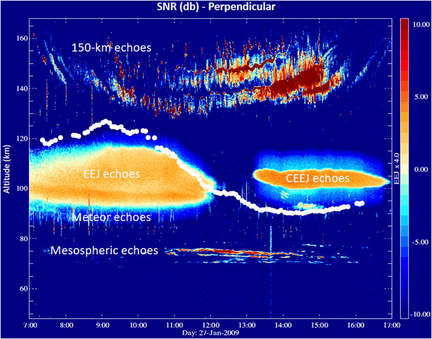
FIGURE 1. Example of an altitude-time signal-to-noise ratio (SNR) of targets over Jicamarca between 65 and 170 km during daytime on 27-January-2009, i.e., 150-km, normal (EEJ) and counter (CEEJ) equatorial electrojet, and mesospheric echoes. The mean vertical E ×B drift from 150-km echoes is overplotted in white (see scale to the right multiplied by 4) (adapted from Reyes et al., 2020, Figure 1).

Figure 2 shows nine consecutive days of SNR observed in January 2009 over JRO. Although the general characteristics of LLVR echoes mentioned above are observed (e.g., necklace, layering, pearls, altitude boundaries), they do present a strong day-to-day variability (Obs10). For example, the necklace shape and regions of strong echoes are not the same from day to day. During this time, the solar conditions were low and the geomagnetic conditions were quiet (e.g., Chau and Kudeki, 2013, for more details). This is another indication that neutral dynamics play a role on their day-to-day variability. More features of this figure are described in Section 8.

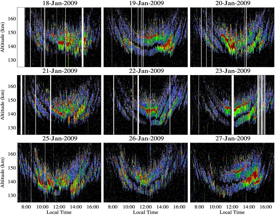
FIGURE 2. Altitude-time SNR observations of 150-km echoes over nine consecutive days in January 2009 over Jicamarca. The color scale is in dB. Very strong echoes (in red) present usually narrow features resembling layers (either ascending or descending) (from Chau and Kudeki, 2013, Figure 2).

Thanks to the high-power large-aperture capabilities at JRO, even higher time resolution measurements can be made. Figure 3 shows high-resolution observations for selected regions of echoes lasting for a few minutes (pearls). These high-resolution observations show that the strength of echoes is also modulated at subminute scales (Obs11). The dominant periods on the selected regions are indicated at the top of each frame. These periods vary between a few seconds to tens of seconds. More details can be found in chapter 5 of Reyes (2017).

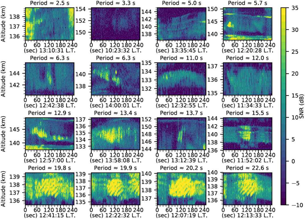
FIGURE 3. High-resolution altitude-time SNR showing examples of sub-minute fluctuations in the 150-km region above Jicamarca on 30-January-2016. Dominant periods for each selected time-altitude window are indicated. (from Reyes, 2017, Figure 5.14).

It is important to note that high-power JRO observations of LLVR echoes have been limited to a few days a year in the last 2 decades. However, thanks to the wide range of SNR, the echoes have been routinely measured at JRO in a low power mode called JULIA (Jicamarca Unattended Long-term investigations of the Atmosphere), namely the large JRO array is used with unattended low power transmitters (e.g., Hysell et al., 1997; Hysell and Burcham, 2002). JULIA observations of 150-km echoes have contributed to study their seasonal behavior, i.e., at JRO the echoes occur at all seasons, and a seasonal variability (Obs11) is observed in the number of layers and altitudinal coverage of the echoes (Chau and Kudeki, 2006b). Furthermore, no correlation was found with concurrent magnetic activity using the K_p index (Matzka et al., 2021). Recently, Yokoyama et al. (2022) has reported a negative correlation between 150-km echo occurrence over Indonesia, but using K_p indices with 1 day delay.

Currently, JULIA 150-km observations constitute the longest database of ground-based vertical and zonal E ×B drifts at the magnetic equator. JULIA drifts have been used to study ionospheric changes at low latitudes during sudden stratospheric warming events (e.g., Chau et al., 2010a), to validate empirical equatorial zonal electric field models based on satellite magnetometer data (e.g., Alken, 2009), or were directly used to develop statistical relations between variations at low latitude magnetometer ground stations and the vertical drift (e.g., Anderson et al., 2004, 2006; Stolle et al., 2008).

The fact that 150-km echoes could be measured with lower power systems and that they provide valuable measurements of the F-region electric fields, motivated the exploration of such echoes at other equatorial and off-equatorial sites. Close to the magnetic equator, successful measurements have been conducted over Pohnpei (e.g., Kudeki et al., 1998; Tsunoda and Ecklund, 2000), and Sao Luis (e.g., De Paula and Hysell, 2004; Rodrigues et al., 2011). Off-equatorial observations have been made over Gandanki (e.g., Choudhary et al., 2004; Patra and Rao, 2006), Indonesia (e.g., Patra et al., 2008; Yokoyama et al., 2009), Christmas Islands (Tsunoda and Ecklund, 2008), and China (e.g., Li et al., 2013). Currently only observations over Gadanki and Indonesia are routinely made.

All of these observations have been made at low VHF frequencies (between 30 and 60 MHz) and with beams pointing perpendicular to B, i.e., observations at 3 to 5 m Bragg wavelengths (Obs13). Using similar frequencies, radar experiments at middle and high latitudes using MU radar (e.g., Fukao et al., 1985) and MAARSY (Latteck et al., 2012), respectively, have not revealed signatures of 150-km echoes, i.e., LLVR echoes appear to be a low latitude phenomena (Obs14) since they have been observed only between ±13° dip latitude.

Figure 4 show altitude-time SNR observations over Gadanki, India (left) and Sao Luis, Brazil (right) for three consecutive days. Although these systems are less sensitive than JRO’s high-power large-aperture mode by more than 10 and 20 dB, respectively, both systems show the general 150-km features, i.e., necklace, layering, minute variability, lower and upper altitude boundaries, day-to-day variability. More details on these observations and the systems used can be found in Patra (2011) and Rodrigues et al. (2011), respectively.

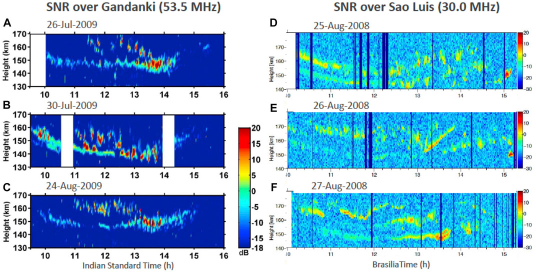
FIGURE 4. Altitude-time SNR observations of 150-km echoes observed over three consecutive days over Gadanki, India (A, B, C) (adapted from Patra, 2011, Figure 3) and Sao Luis, Brasil (D, E, F) (adapted from Rodrigues et al., 2011, Figure 3). Note that in 2008 Sao Luis was located at the magnetic equator.

The Sao Luis observations were made at 30 MHz with a much smaller antenna array than Gadanki’s and JRO’s arrays. Although frequency dependence of ionospheric plasma irregularities have been observed in other ionospheric echoes (e.g., Balsley and Farley, 1971), the strength of the reported echoes was unexpected. In Section 6, we elaborate more on the frequency dependence of the echoes.

Observations at sites with beams pointing perpendicular to B but at relative large east and west angles, show a persistent feature in 150-km echoes, East echoes are stronger than West echoes, i.e., perpendicular echoes present a zonal asymmetry (Obs15) (e.g., Kudeki et al., 1998; Tsunoda and Ecklund, 2000, 2008; Yokoyama et al., 2009; Pavan Chaitanya et al., 2018). Figure 5 shows an example of 150-km echoes observed over Indonesia with the EAR (Equatorial Atmosphere Radar) using four beams in the zonal plane perpendicular to B. The echoes are consistently stronger in the East beams. Yokoyama et al. (2009) attributed this asymmetry to arc structures in the plasma instabilities responsible for the echoes.

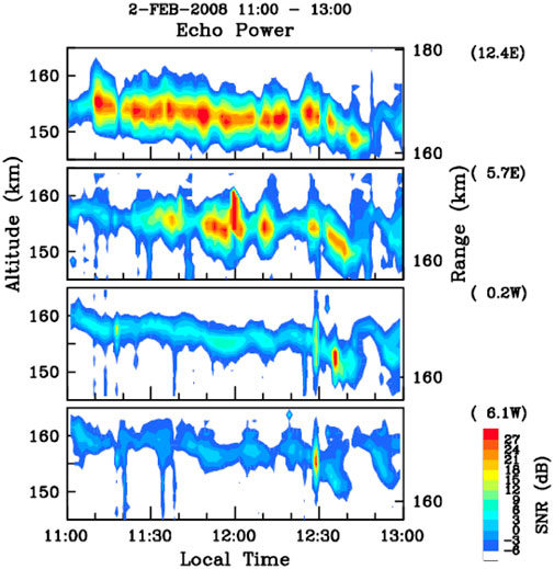
FIGURE 5. Altitude-time SNR plots of 150-km echoes observed at different zenith angles over the Equatorial Atmosphere Radar, Indonesia on 02-February-2008 (from Yokoyama et al., 2009, Figure 3).

At JRO, oblique observations are limited to ±2° in the zonal direction. Multi-beam experiments in the East-West direction using these small angles have not revealed the asymmetry reported at other sites (Fawcett, 1999).

4 Radar observations off-perpendicular to B

Until 2004, 150-km echoes were identified only in experiments using beams perpendicular to B, presented narrow spectral widths, and therefore were attributed to FAIs. Chau (2004) reported the first observations of 150-km echoes with beams pointing a few degrees with respect to B (oblique observations) using JRO’s high-power large-aperture capabilities. The experiments were not planned to study LLVR echoes, they were aimed to study meteor head echoes (Chau and Woodman, 2004b) and simultaneously obtained drifts from 150-km Doppler shifts with a newly developed acquisition system at the time. The latter was expected to be obtained from echoes observed with JRO’s antenna sidelobes as it was done in Aponte et al. (1997), but using a pulse-to-pulse spectral analysis. Serendipity took place and besides the expected narrow spectra, off-perpendicular to B echoes showing wide spectra (Obs16) were observed. Since the experiments were performed with relatively long IPPs, the spectra were frequency aliased. Non-etheless, they were at least 100 times wider than perpendicular to B spectra. Although Chau (2004) identified the first oblique 150-km echoes, they had been already present in standard oblique incoherent scatter measurements at JRO, but were confused with 150-km echoes coming from antenna sidelobes pointing perpendicular to B (Aponte et al., 1997).

Altitude-time observations of oblique 150-km echoes showed similar features to the perpendicular ones, i.e., daytime occurrence, necklace shape, upper and lower altitude boundaries, layering, minute-scale structures (e.g., Chau, 2004, Figure 3). The strength of these echoes were reported to be 2-3 orders of magnitude weaker than those from perpendicular echoes, based on SNR measurements. In retrospective, this statement has been misleading, since the SNR of oblique echoes given that their spectra is much wider, will be much smaller than the SNR of perpendicular echoes for the same signal (S). In other words, the strength of oblique echoes is comparable to those from perpendicular beams, but their total noise is larger.

The initial connection to the traditional 150-km echoes was made indirectly just by comparing altitude-time SNR features. A series of experiments were conducted at Jicamarca aimed to better characterize these echoes and to try to understand their origin. For the latter, high-resolution electron density (N_e) measurements using incoherent scatter techniques were performed to see if there were enhanced narrow layers of N_e. These experiments did not reveal a significant enhancement on N_e (e.g., Chau et al., 2010b).

Chau et al. (2009) performed simultaneous perpendicular and oblique experiments aimed to characterize the oblique spectra and the altitude-time behavior of both echoes. They performed basically two experiments with simultaneous perpendicular and oblique beams: (a) with volumes separated by a couple of kilometers in the north-south direction at 150 km altitude, and (b) common volume. The former was performed by using different sections of the main JRO array, while the latter was performed with the aid of a small receive-only array located a few kilometers south of JRO. Figure 6A shows the geometry used for both experiments. Both of these experiments were performed with short IPPs to avoid frequency aliasing of the oblique wide spectra at the expense of F-region range-aliased incoherent scatter echoes. The range aliased echoes contributed to increase the noise of 150-km echoes, but not to change their shape.

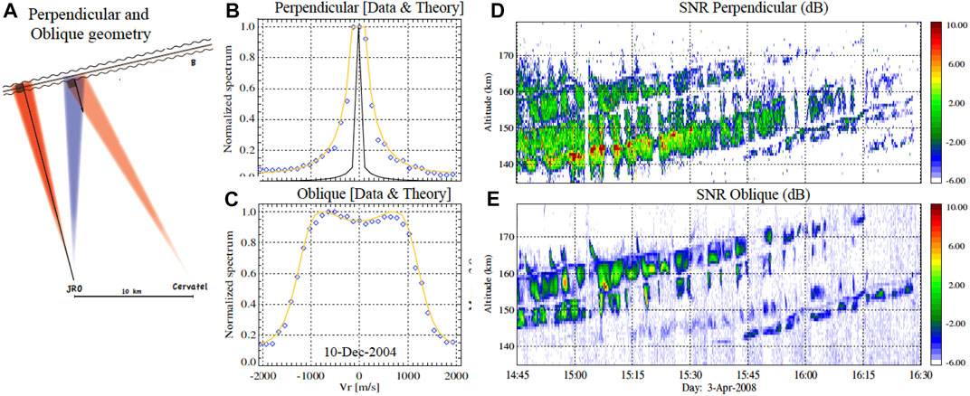
FIGURE 6. Simultaneous perpendicular and oblique observations of 150-km echoes over Jicamarca between 2004 and 2008: (A) Monostatic and bistatic geometries for perpendicular (red) and oblique (blue) beam; 3-min measured normalized-to-the-peak spectrum (blue circles) at 160 km for (B) perpendicular and (C) oblique on 10-December-2004; altitude-time SNR for (D) perpendicular and (E) oblique beams on 03-April-2008. Note that in (B,C) fitted incoherent scatter spectra are indicated in solid orange lines. In (B), the normalized spectra is shown with (black) and without (blue) low frequency components (adapted from Chau et al., 2009, Figures 1, 5, 6).

Figures 6B, C show examples of spectra observed with the common volume perpendicular and oblique beams, respectively, after 3 minute integration time. In both figures the blue dots represent the normalized spectra by interpolating the zero-Doppler spectral bin, while the orange line represents the fitted spectra using incoherent scatter theory described in Kudeki and Milla (2006). The solid line in Figure 6B shows the normalized spectra including the zero-Doppler spectral bin. Both spectra qualitatively conform with the expected spectra of an ionosphere in thermal equilibrium, i.e., the spectra predicted by incoherent scatter theory at angles close to perpendicular to B (e.g., Sulzer and González, 1999; Woodman, 2004; Kudeki and Milla, 2012). Namely the spectra are wide/narrow at oblique/perpendicular angles and they are dominated by the ion/electron dynamics. Moreover the spectral width of the oblique echoes increases with increasing altitude, as expected for this region (Chau et al., 2009, Figure 5). One could be tempted to routinely fit the observed oblique spectra with incoherent scatter theory to get temperatures and composition, but a better understanding of the physics governing these oblique echoes is still needed.

The two-beam experiments confirmed the connection made earlier by Chau (2004), i.e., oblique 150-km echoes are related to the traditional perpendicular ones. However, the connection is valid for the majority of echoes, not for all. Figures 6D, E show the simultaneous observations of perpendicular and oblique 150-km SNR, respectively. The two salient features of these two figures are: (a) all oblique echoes are accompanied by perpendicular ones (Obs17), (b) simultaneous oblique and perpendicular echoes are the majority (Obs18), and (c) there are regions of only perpendicular to B echoes (Obs19). More examples of these features can be found in Chau et al. (2009), where perpendicular-only echoes can be observed at layers where oblique echoes are observed, but not at the same time (e.g., Chau et al., 2009, Figure 2).

Comparing calibrated returned signals from these two-beam experiments and performing experiments at larger angles with respect to B, Chau et al. (2009) reported that the oblique echoes present a north-south aspect sensitivity (Obs20) that in general varies with altitude (being less aspect sensitive at upper altitudes (Chau et al., 2009, Figure 4). Previously using radar interferometry in the north-south direction, perpendicular 150-km echoes were reported to be highly aspect sensitive (e.g., Fawcett, 1999; Lu et al., 2008). The oblique observations indicate that the majority of echoes are not high aspect sensitive. However, previous perpendicular observations can be understood given the strong spectral dependence on pointing angle with respect to B. As in the case of incoherent scatter theory, low-frequency spectral components will be highly aspect sensitive, i.e., most of the power of the perpendicular spectra is concentrated in low frequency bins (electrons dominating the spectra). Such angular dependence of incoherent scatter spectra at small angles with respect to B have been used to measure the B inclination at ionospheric heights (Woodman, 1971).

Given that the oblique echoes also show minute-scale SNR variability (e.g., Figure 6D), in Figure 7 we show the time evolution of normalized oblique spectra in lineal scale, at two selected altitudes, i.e., 160 (top) and 145 (bottom) km, observed on 10-December-2004 (e.g., Chau et al., 2009, Figure 2). Although the 3-minute integrated oblique spectrum shows the expected symmetric double-hump (see Figure 6C), the higher time resolution spectra show a time variability of their spectral peaks, showing spectral asymmetry with sub-minute to minute variability. As in the case of incoherent scatter spectra asymmetries observed at high latitudes (e.g., Fontaine and Forme, 1995), field-aligned currents might be behind the observed asymmetry in 150-km oblique echoes.

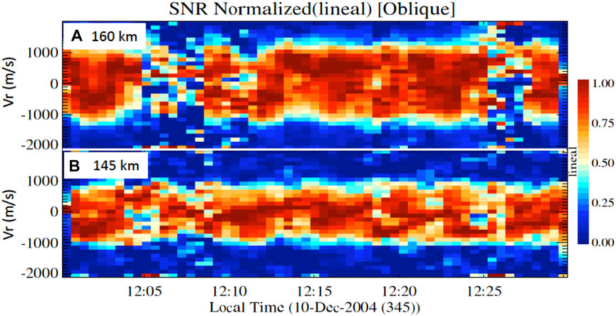
FIGURE 7. Normalized spectrograms of oblique 150-km observations at (A) 160 km and (B) 145 km. These spectra were obtained with high temporal resolution observed over Jicamarca on 10-Dec-2004, i.e., same data used in Chau et al. (2009) and Figure 6B. Note the sub-minute to minute variability of the spectra peaks.

Based on the spectral features of the two-beam experiment, Chau et al. (2009) associated the oblique echoes (and their perpendicular counterpart) to some kind of naturally enhanced incoherent scatter (NEIS) echoes. On the other hand, the perpendicular-only echoes were associated to FAIs. In both cases, echoes are a few orders of magnitude stronger than expected echoes from plasma in thermal equilibrium.

5 Types of echoes, seasonal and solar variability

To further characterize 150-km echoes in terms of day-to-day, seasonal and solar variability, additional two-beam observations would have been ideal. However, those observations are limited to JRO and to a handful of days. The former is due to the lack of enough power-aperture at other radars located at low latitudes. Common volume two-beam experiment at JRO were only possible during a special campaign where a receive only station was installed for a few weeks south of JRO. The main purpose of the additional array was to study meteor echoes (Malhotra et al., 2007). Additional two-beam experiments using only the JRO array as described in Chau et al. (2009), i.e., with short IPP, have not been performed frequently since they are useful only for 150-km studies, and there has been more demand to study more than one region simultaneously, e.g., the so-called MST-EEJ-ISR or multiple-beam ISR modes (e.g., Milla et al., 2013; Lehmacher et al., 2020).

In this section we return to the routine observations made with perpendicular beams. Motivated by the localized strong echoes in altitude-time plots of SNR, Patra (2011) and later Chau and Kudeki (2013) investigated the relationship between SNR and spectral width of perpendicular echoes over Gadanki and JRO, respectively. Based on the 2D histogram distributions as a function of these parameters, they found two main populations and named them type A and type B echoes (Obs21), i.e., in type A echoes the SNR (in dB) is linearly dependent on spectral width, while in type B echoes the SNR is almost independent of spectral width. Furthermore, over Gadanki and JRO, type A echoes are the majority (Obs22) and they are 1–3 orders of magnitude weaker than type B echoes.

Figure 8 shows selected examples taken over JRO (left) and Gadanki (right) during: low (top) and medium (bottom) solar flux conditions. The results of Figure 8A were obtained from the observations shown in Figure 2.

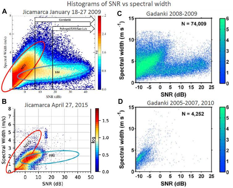
FIGURE 8. Two-dimensional histograms of 150-km echoes based on SNR and spectral width, for Jicamarca (A, B) and Gadanki (C, D) and low (A, C) and moderate (B, D) solar conditions. Two-distinct populations are identified in 2009, while at other years (solar conditions), the type B (FAI) population is less over both sites (adapted from Chau and Kudeki, 2013; Reyes, 2017; Patra and Pavan Chaitanya, 2016, Figures 3, 3.16, 5, respectively).

Based on the clear but short two-beam experiment dataset (see Section 4), Chau and Kudeki (2013) suggested that the populations from the two-beam datasets (i.e., oblique and perpendicular echoes) and from the SNR and spectral width distributions, were associated. Namely, type A echoes were associated to NEIS, and type B to FAIs. By incoherent scattering they were referring to the association to incoherent scatter radar theory. Similar type of incoherent scatter enhancements are found at high latitudes called NEIALs (Naturally Enhanced Ion-Acoustic Lines) (e.g., Rietveld et al., 1991; Kontar and Pécseli, 2005), although they might not be physically related to 150-km NEIS.

The association of type A to NEIS is also supported by the expected spectral behavior at angles close to perpendicular to B. Since beams pointing perpendicular to B are finite, the resulting spectra will be a convolution of spectra signatures from different angles with respect to B within the observing beam. From Figure 6B, one can see that for weak signals the spectral width will be dominated by the signals coming exactly perpendicular to B (narrower spectra), while as the signal increases, the signals from the oblique angles start to contribute, increasing the measured spectral width. This is particularly true if a simple spectral moment or single Gaussian fitting methods are used. In cases where larger volumes (beam width and range resolution) are used (e.g., over Gadanki), the resulting spectra might be a convolution of both type of echoes occurring at different altitudes. Patra et al. (2020b) have shown that a simple moment method could be misleading on such occasions and suggested a classification considering also the frequency spread of the echoes. Perhaps a two-Gaussian fitting procedure would be more appropriate under these circumstances, i.e., one for the narrow spectral region with large amplitude and one for the wider region with less amplitude.

In the case of type B, echoes coming from FAIs are expected to be narrow and their SNR to be strong, given their longer correlation times. Patra (2011) suggested that intermediate layers with perhaps metallic ions, might be creating small density gradients and conditions for FAIs to occur.

The SNR and spectral width estimations should be considered as relative quantities, since they depend on the acquisition parameters (e.g., effective bandwidth), background noise (e.g., passing of the center of the Galaxy), estimation parameter (e.g., moments or Gaussian fitting). Non-etheless, all four examples in Figure 8 provide a qualitative separation of populations. A striking feature in this figure is that in both JRO and Gadanki, type B echoes occur more often during solar minimum conditions, i.e., there is a strong solar variability in type B echoes (Obs23) (see also, Patra and Pavan Chaitanya, 2016; Reyes, 2017).

Figure 8A also shows qualitatively that smaller systems like Pohnpei, Sao Luis, EAR, etc. being less sensitive than JRO’s high-power large-aperture modes, would be mainly sensitive to type B echoes. On the other hand, Gadanki should be sensitive to both type of echoes, as shown in Figures 8C, D.

The routine observations at the low-latitude stations mentioned above and JULIA 150-km observations at JRO have shown that 150-km echoes present a seasonal variability that appears to vary depending on the type of echo, longitude and perhaps latitude. For example, echoes occur: (a) mainly in the summer over Pohnpei (Tsunoda and Ecklund, 2000), (b) more often and stronger during solstices than equinoxes over Indonesia (Pavan Chaitanya et al., 2018), (c) more frequently in June solstice over Gadanki for both type A and B (Patra and Pavan Chaitanya, 2014), (d) all year without a strong seasonal dependence over Sao Luis (Rodrigues et al., 2011), (e) all year without a strong seasonal dependence over JRO with JULIA mode (Chau and Kudeki, 2006b). Except for JULIA and Gadanki, the reported seasonal results in the other systems are most likely for type B echoes.

As in the case of seasonal dependence, the solar cycle dependence have been also studied at different sites. As shown in Figure 8, type B echoes are more frequent during solar minimum conditions over JRO and Gadanki. Echoes over EAR also show a strong solar cycle dependence, they are stronger during solar minimum conditions (Yokoyama et al., 2022). Given the sensitivity of EAR, this solar dependence is most likely only applicable to type B echoes.

Are the physics of type A and type B related? Do echoes from NEIS and FAIs have some physics in common? We come back to these questions in Section 9.

6 Multi-frequency radar observations

Previously we mentioned that the 150-km echo observations made with the relatively small Sao Luis radar (De Paula and Hysell, 2004; Rodrigues et al., 2011) were surprising, suggesting a strong frequency dependence of the echoes. Patra et al. (2018) presented the first co-located observations of 150-km echoes over Gadanki at 30 and 53 MHz. Figure 9 shows SNR examples taken during four consecutive days during summer solstice with the 30 (left) and 53 (right) MHz systems. These initial observations were collocated but made with different volumes and transmitted power, i.e., 53 MHz observations were made with a smaller volume (larger array) and more power than 30 MHz observations. Despite the differences, one can observe a clear qualitative frequency dependence (Obs24) of the echoes. The majority of strong 30-MHz echoes are not observed in the 53 MHz system, some strong 53-MHz narrow layers are observed in the 30 MHz system. Using a 2D histogram based on SNR and spectral width, type B echoes are more frequent than type A in the 30 MHz observations, contrary to what has been observed in previous 53 MHz observations (e.g., Patra et al., 2017, Figure 3).

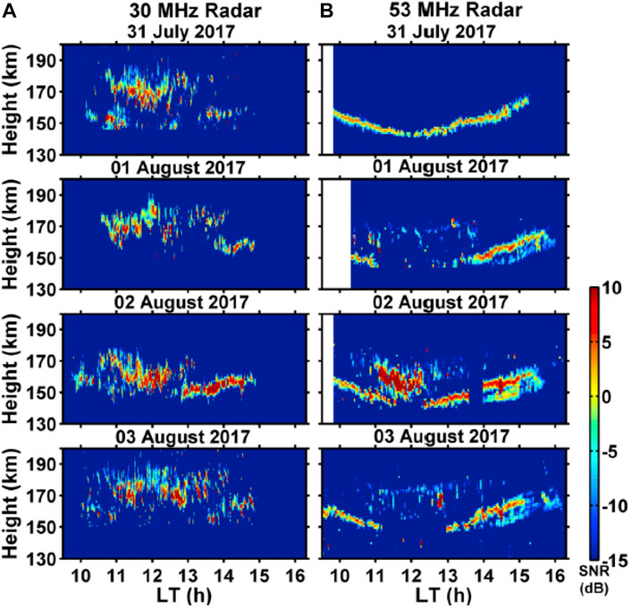
FIGURE 9. Altitude-time SNR co-located observations of 150-km echoes between 31-July-2017 and 03-August-2017 over Gadanki at: (A) 30 MHz and (B) 53 MHz (adapted from Patra et al., 2018, Figure 1).

Common-volume 53- and 30-MHz observations confirmed that type B echoes have a strong frequency dependence. Patra et al. (2020a) accomplished that by reducing the transmitter power and antenna size of the 53 MHz radar, i.e., comparing only the strong 53 MHz signals with the 30 MHz signals. Although not explicitly mentioned in the Gadanki papers, these results suggest that indeed there is a frequency dependence, and the dependence is stronger in type B echoes than in type A. The frequency dependence of 150-km echoes seems to be large, favoring lower VHF frequencies. Perpendicular as well as oblique observations of the valley region with the low latitude ALTAIR VHF/UHF (∼150, ∼422 MHz) radars have not shown any indication of power enhancements around 150-km altitudes (e.g., Kudeki et al., 2006; Milla and Kudeki, 2006).

Observations of the daytime LLVR have also been pursued with a high-resolution HF radar over Africa. Echoes coming from 150-km virtual height were suggested to be part of the 150-km echoes observed at VHF (Blanc et al., 1996). However based on recent measurements with a high-resolution ionosonde and HF-beacon network around Jicamarca (e.g., Hysell et al., 2016), echoes around 140–160 km virtual height, are most likely coming from low elevation EEJ kilometer-scale echoes.

7 Electron densities and 150-km echoes

As mentioned above, the valley region is difficult to observe using both ground- and space-based instruments. Radar echoes have been the most common way to observe the region. Recent advances in ionosonde technology has yielded higher time, frequency and range resolutions allowing the exploration of this region of low N_e. In Figure 10 we show concurrent measurements of 150-km echoes with the high-power large-aperture 50-MHz radar at JRO and a modern ionosonde called a VIPIR (Vertical Incidence Pulsed Ionospheric Radar). Figure 10A shows high-resolution 150-km echoes and the temporal variations of gap regions (forbidden zones) with solid color lines. The solid yellow lines represent their smoothed series. Figure 10B shows the simultaneous virtual height measurements with VIPIR for different reflecting frequencies (i.e., N_e contours). The high-frequency gap times series in Figure 10A are overplotted on frequency contours with the highest correlation. These results shows that 150-km features are connected to electron densities (Obs25). Previously Tsunoda and Ecklund (2007) and Chau et al. (2010b) suggested that 150-km echoes were connected to the F₁ electron density peak and N_e changes, but without explicitly indicating what features in N_e correspond to 150-km echoes.

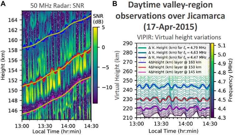
FIGURE 10. Daytime valley region observations over Jicamarca on 17-April-2015: (A) 150-km SNR with Jicamarca 50 MHz radar, and (B) VIPIR virtual height reflections. In (B) reflecting frequencies are color coded. Solid color curves magenta, red and blue show the oscillations of the wide gaps in (A) representing forbidden layers around 145, 150, and 160 km, respectively. Their corresponding fluctuations are overplotted to VIPIR virtual heights in (B) (adapted from Reyes et al., 2020, Figures 11, 13).

Although ionosondes at low latitudes have been operating for more than 80 years, high frequency, range, and temporal resolution measurements needed to characterize the LLVR have recently become available with modern ionosondes. The VIPIR system at Jicamarca consist of a wide-band log-periodic antenna that transmits vertically propagating radio wave pulses with a 4-kW peak power transmitter capable of sweeping its frequency from 0.3 to 20 MHz. The results presented here were taken by sweeping the frequency from 1.6 to 12.5 Mhz on a pulse-to-pulse basis over a period of 10-s duration. The reflected pulses from the ionosphere were detected using eight short dipoles arranged in two orthogonal sets of interferometric baselines. Despite the advances in hardware, automatic processing of the new high-resolution ionosonde measurements are still not possible, therefore manual detection analysis was needed. Some of the challenges particularly for the LLVR are: (a) strong daytime EEJ scattering making the F₁ traces fuzzy, (b) E-region peak N_e blinding upper altitudes with lower densities, and (c) the highly altitudinal and temporal N_e variations of the region. More details on these radar and VIPIR LLVR studies and their challenges can be found in Reyes et al. (2020).

The connection of 150-km echoes with both electron densities values and variations have been independently reported during special geophysical conditions. Temporal and altitudinal features of 150-km echoes vary significantly during solar flares (Obs26) (see Figure 11A). For example: (a) the lower boundary is moved to even lower altitudes for a short time, (b) the gap regions (forbidden zones) change significantly, (c) distances between layers are reduced (e.g., Reyes, 2012). Pedatella et al. (2019) simulated the solar flare effects of 07-September-2005 over JRO, using the WACCM-X (Whole Atmosphere Community Climate Model with thermosphere-ionosphere eXtension). Figures 11A, B show the JRO observations and the WACCM-X N_e, respectively. The results show that indeed 150-km echo structure follows changes in N_e. Furthermore, Pedatella et al. (2019) were also able to simulate the observed vertical drifts during this event, pointing to the importance of conductivity changes locally and along the B lines connecting to the E region.

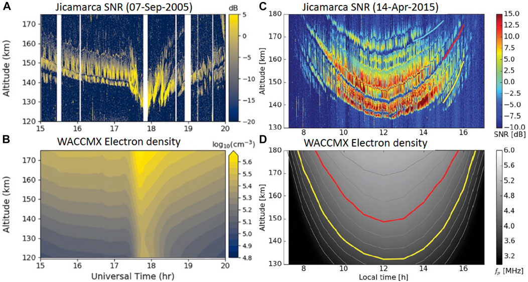
FIGURE 11. SNR observations of 150-km echoes over Jicamarca on (A) 07-September-2005 and (C) 14-April-2015 and their corresponding simulated electron densities by the Whole Atmosphere Community Climate Model with thermosphere-ionosphere eXtension (WACCM-X) shown in (B, D), respectively. White areas in (A) indicate time periods without observations. The 07-Sep-2005 observations corresponds to a solar flare event. Yellow and red lines in (D) corresponds to 3.9- and 4.5-MHz contours, they in turn appear to corresponds to the wide gaps in (C) (adapted from Pedatella et al., 2019; Lehmacher et al., 2020, Figures 1, 4, respectively).

Further WACCM-X simulations have been used by Lehmacher et al. (2020) to study 150-km echoes with high-power large-aperture modes over JRO, therefore allowing the observations of echoes and features not observed at other lower sensitivity radars. The results also show that general features of 150-km echoes follow N_e contours. Figures 11C, D show 150-km echoes over JRO and WACCM-X N_e contour, respectively. By combining observations and Ne modelling for different seasons and solar conditions, Lehmacher et al. (2020) show the seasonal and solar cycle variability of the wide gap altitudes and the separation between gaps to absolute values of N_e (or plasma frequencies).

The wide gaps appear to happen when the upper-hybrid frequency is an integer multiple of the electron gyrofrequency. Using values from the IGRF (International Geomagnetic Reference Field) model for 2015 (Alken et al., 2021), the electron gyrofrequency is ∼0.652 MHz. For the particular example of 14-April-2015, those lines are indicated in red and yellow in Figures 11C, D and corresponds to contours of ∼3.9 and ∼4.5 MHz, respectively (see, Lehmacher et al., 2020, for more details).

Observations of LLVR echoes have also shown a peculiar response during a solar eclipse (Obs27) (see Patra et al., 2011, Figure 1). Patra et al. (2011) reported the presence of 150-km echoes over Gadanki during the solar eclipse of 15-January-2010. Before/after the central time of the eclipse the observed echoes were ascending/descending in altitude as function of time. These observations were complemented with ionosonde observations showing electron densities ascending/descending before/after the central time of the eclipse.

8 Physical mechanisms: Modeling and theory

Here we review the different suggestions that explain LLVR echoes, with a particular emphasis on recent modeling and theory developments that solve some of the key riddles behind these echoes. Before discussing those suggestions and developments, in Table 1 we summarize the main observational features associated to LLVR echoes. Each of the features have been mentioned in the text above and selected references are included in the table. To help the reader, we also include the numbers of the figures used in the paper that support the majority of those observational features.

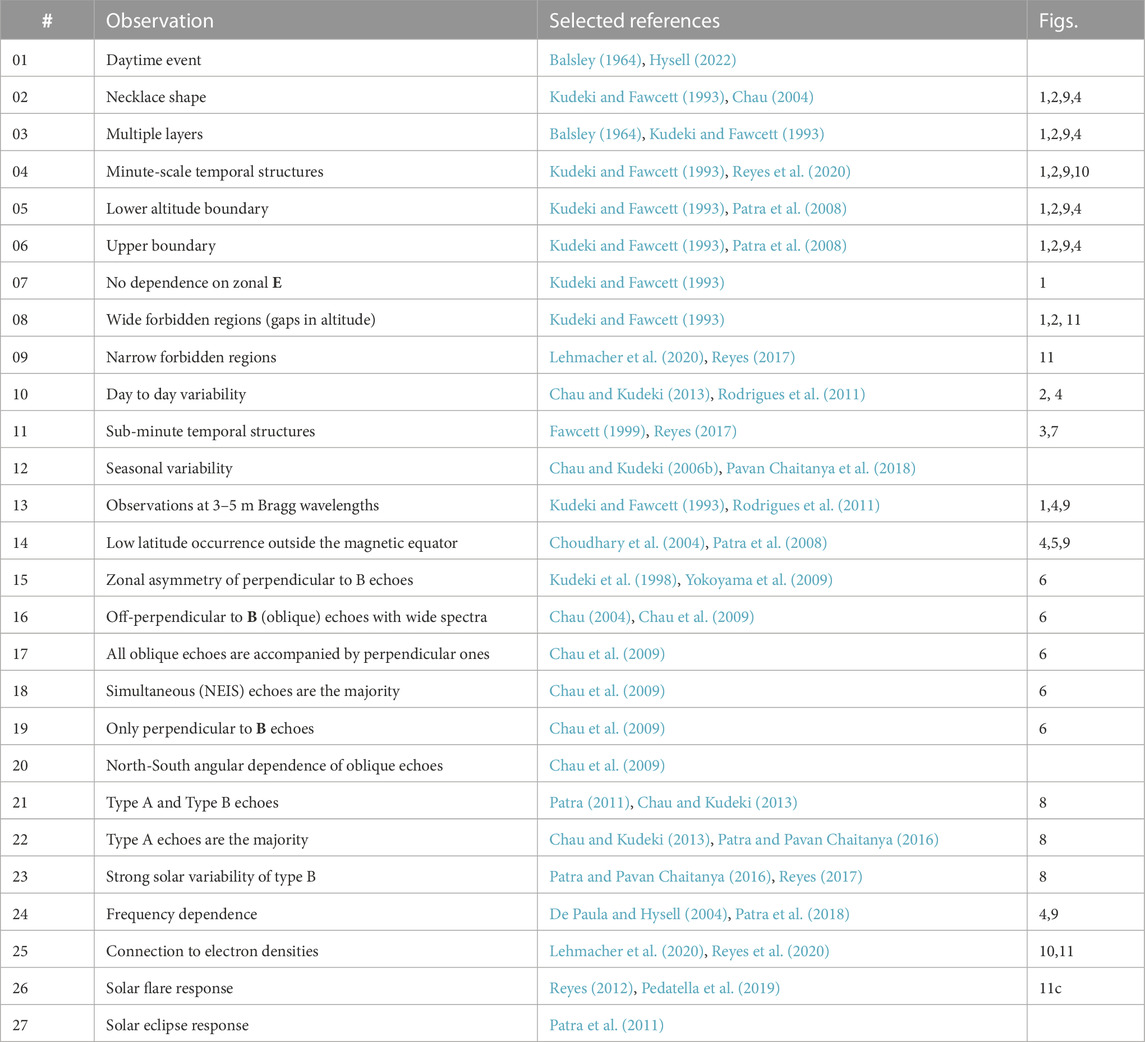
TABLE 1. Summary of main 150-km observed features, including selected references and figures in this work supporting the observations.

Instead of making a chronological description, in this section we start with the latest modeling and theoretical results, and later list additional aspects that have been suggested to contribute to the understanding of the echoes.

8.1 Photoelectron induced waves

Motivated by the necklace shape (Obs01) and sudden changes in 150-km echo morphology during a solar flare event (Obs26), Oppenheim and Dimant (2016) investigated the role of photoelectrons in 150-km echoes. A few measurements of photoelectron distributions have shown that between 120–180 km, multiple photoelectron peaks at 5 eV and 22–27 eV exist during the day (e.g., Lee et al., 1980; McMahon and Heroux, 1983).

Their study used kinetic 2-D and 3-D Electrostatic Parallel Particle-in-Cell (EPPIC) simulator (Oppenheim and Dimant, 2013) with a population of photoelectrons. This setup simulates the dynamics of charged particles as they respond to internally generated electric fields with a constant background B. The EPPIC simulations show that the photoelectrons lose energy to electron plasma waves faster than they lose energy due to collisions with neutrals.

Figure 12 show the normalized spectra of electron density fluctuations for three different angles with respect to B (columns) and two runs: (top) background without photolectrons, and (bottom) baseline with photolectrons. The simulations reproduce wide ion-line spectra at angles slightly off-perpendicular to B and narrow spectra perpendicular to B, for both background and baseline simulations.

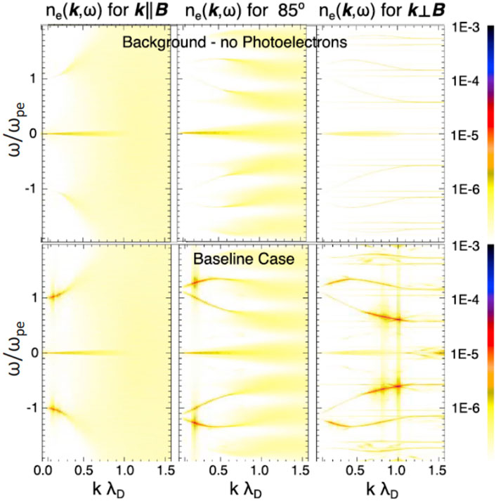
FIGURE 12. Electron density spectra at a range of angles with respect to B: (top row) without photoelectrons (“noise case”), and (bottom row) with photoelectrons (baseline case). The frequency is normalized to the plasma frequency (ω_pe), and the wave number is normalized to the Debye length (λ_D) (from Oppenheim and Dimant, 2016, Figure 4).

The energy from the slowing photoelectrons goes into electron waves via inverse Landau and cyclotron damping (e.g., Oppenheim and Dimant, 2016, movie in their supporting information). Comparing the spectra for the two runs shows that energy goes both into plasma waves parallel to B and harmonics of the cyclotron frequency (electron Bernstein modes). These spectra should account for enhanced plasma lines as observed by radars. Even in an undisturbed warm plasma, large incoherent scatter radars receive reflections from thermal fluctuations of ion-acoustic waves, allowing measurements of plasma density, temperature, and composition (e.g., Kudeki and Milla, 2012). To explain majority of 150 km echoes, i.e., NEIS echoes, one needs a ∼10 dB enhancement of low-frequency waves above the background thermal fluctuations at the radar wavelength. Zooming in Figure 12 around the ion-line, the baseline simulations predict just such an enhancement driven by the electron waves. Moreover, enhancements in the ion line are evident at low frequencies (i.e., wavelengths close to 3 m).

Based on these simulations, Oppenheim and Dimant (2016) proposed that 150 km echoes originate due to a multistep process that exists at around 150 km altitude. At these altitudes, UV photons ionize O₂ or N₂ molecules, creating electrons with energies greatly exceeding the ambient plasma thermal energy of ∼0.03 eV. These photoelectrons will form a bump-on-tail population, but since the distribution is isotropic in 3-D, the bump takes the form of a phase space shell. In an unmagnetized plasma, such a shell should not produce an instability, but the magnetic field breaks the symmetry of the system and leads to energetic particle-driven wave growth through inverse Landau and cyclotron damping. In particular, the shell interacts with the background electrons to generate upper hybrid, electron Bernstein, and Langmuir waves. These electron waves then couple to oblique ion-acoustic waves, perpendicular ω = 0 modes, and lower hybrid modes, generating irregularities that radars detect as 150 km echoes.

This model explains the following features of 150-km echoes:

• (Obs01) They occur only during the day.

• (Obs02) Their necklace shape, since EUV photons penetrate most deeply at noon.

• (Obs13) Observations at 3–5 m Bragg wavelengths, given that high-frequency electron modes decay non-linearly into ion waves, enhancing structures around 3 m wavelengths.

• (Obs16) The existence of oblique echoes with wide spectra.

• (Obs17) All oblique echoes are accompanied by perpendicular ones, i.e., NEIS echoes.

• (Obs26) Their enhancement during a solar flare (Reyes, 2012).

• (Obs27) Their response during a solar eclipse (Patra et al., 2011).

Oppenheim and Dimant (2016) suggested that by invoking resonances the model could explain the layering (Obs03). These resonances could optimize this process at some altitudes and not others, though this argument was not worked out analytically until Longley et al. (2020). Furthermore, they expected that type A echoes (spectral width dependence on SNR) are part of their model results. However, fully testing this hypothesis would require a large number of simulations.

To test this model, Oppenheim and Dimant (2016) suggested that one should compare “solar EUV emission strength with 150 km echo amplitudes.” The solar flux results mentioned above presented by Patra et al. (2017) and Yokoyama et al. (2022), showed that 150-km type B echoes over Gadanki and EAR, respectively, are more frequent and stronger during solar minimum conditions when averaged over a year of measurements. However, the kinetic simulations do not start with photoelectron density but, instead, with an electron velocity distribution, where the detailed structure of that distribution impacts the resulting ion turbulence level and the expected radar echoes. These measurements indicate that higher EUV/X-ray intensities do not necessarily create more unstable photoelectron distribution functions needed to create higher annually averaged occurrence rates of 150-km echoes at the particular altitudes where these radars detect them. The anticorrelation between EUV and echo occurance rate shows the complexity of the system that creates NEIS echoes from photoelectrons. The dramatic changes in 150-km echoes during solar flares also reinforce this point. Lastly, the photoelectron-driven kinetic model does not yet explain type B echoes.

8.2 Photoelectron-driven upper hybrid instability

The pioneering work of Oppenheim and Dimant (2016) as well as the brainstorming discussions at the International Space Science Institute (ISSI) as part of a team to investigate the low-latitude valley region, motivated Longley et al. (2020) to develop a kinetic theory behind photoelectron waves.

The kinetic theory for photoelectron-induced instabilities in the valley region had been previously developed by Basu et al. (1982) and Jasperse et al. (1995). One of the instabilities analyzed in Basu et al. (1982)) is the upper-hybrid instability (UHI), which is generated by inverse Landau and cyclotron damping of a photoelectron bump-on-tail. Jasperse et al. (1995) calculated positive growth rates in the valley region but did not show how the prevalence of the instability can evolve over the day.

Longley et al. (2020) followed these formulations and relaxed the assumptions that limited the applicability of the theories developed by Basu et al. (1982) and Jasperse et al. (1995) in the valley region. Their solution for the thermal population were similar, finding that the primary normal mode is the upper-hybrid (UH) frequency (ω_UH) (Basu et al., 1982), i.e.,

and the primary damping is the collisional damping with a rate,

where ω_pe is the plasma frequency, Ω_e = eB/m is the electron gryrofrequency, ν_m is the collision rate of thermal electrons, and m and q are the electron mass and charge, respectively. The collision rate includes the electron-ion collisions of molecular and atomic species as well as the electron-neutral collisions.

The original expressions in previous works were not valid for regions where ω_UH ≈ nΩ_e, which is important for LLVR since the density and therefore ω_pe change with altitude. Therefore, the dielectric functions describing the growth and damping rates needed to be reevaluated. The modified dielectric function when ω_UH = nΩ_e, allows for thermal electrons to Landau and cyclotron damp the UH waves. This new expression does not change the calculation of the UH frequency (Eq. 1) or collisional damping (Eq. 2), however it adds the effect of Landau damping by thermal electrons to the instability, with a damping rate given by (Longley et al., 2020, Eq. 12),

where $v_{th}=\sqrt{2KT/m}$ is the thermal speed, and K the Boltzmann constant. The argument of the exponential is y_n = (ω_r − nΩ_e)/(k_‖v_th), and therefore the thermal Landau damping is maximized when y_n = 0 or equivalently ω_r = nΩ_e.

The UHI happens when the resonance condition of ω_UH − k_‖v_‖ − nΩ_e = 0 occurs for a v_‖ within the right part of the photoelectron distribution. This resonance condition allows the photoelectron population to inverse Landau damp (including cyclotron damping for n ≠ 0) and enhance the UH waves, causing an instability. Collisions between photoelectrons and neutrals are infrequent on timescales of 1/ω_UH and are neglected. The growth rate of the photoelectron term (γ) is given in Eq. 4 of Longley et al. (2020). The derived expression corrects an error in the factor nΩ_e/ω_UH in Basu et al. (1982) that underestimated the growth rate by 10%–20%. Specific details of the derivation of the three growth and damping rates, i.e., γ, γ_v, and γ_Ld, are found in Longley et al. (2020).

Figure 13 shows the results of the derived UHI theory using WACCM-X neutral and ionized parameters for a selected day. The results for a single photolectron peak at E_o = 5 eV driving the UHI at λ = 20 cm wavelengths for (a) updamped instability (γ), (b) collisional damping rate (γ_v), (c) thermal Landau damping rate (γ_Ld), and (d) total growth rate. The combined effect of photoelectron peaks exciting the UHI at a variety of wavelengths is shown in Figure 13E, with overlaid contours of ω_UH/Ω_e that come from the condition of y_n = 0 that maximizes γ_Ld. Note that, these results were obtained assuming the same photoelectron distribution for the whole day and for all altitudes.

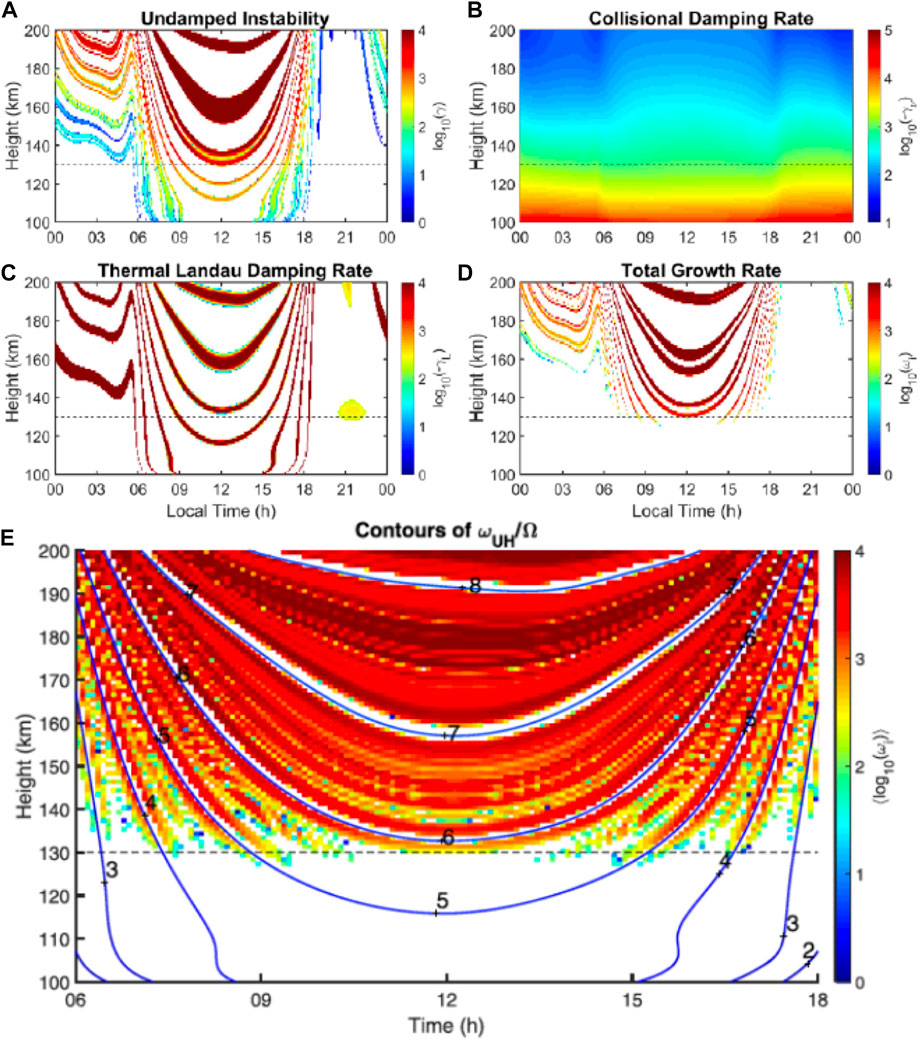
FIGURE 13. (A–D) contribution of different terms to the overall growth rate of the upper hybrid instability (UHI), with E₀ = 5 eV, λ = 20 cm, and α = 2°, namely: (A) Undamped instability (γ), (B) collisional damping rate (γ_v), (C) thermal Landau damping rate (γ_Ld), (D) total growth rate. (E) The summation of growth rates for multiple wavelengths between 20 and 30 cm. The colored regions show where the UHI will occur. The contours of ω_UH/Ω_e are plotted (blue), showing that gaps in the instability occur where ω_UH ≈ nΩ_e. The horizontal dashed line in each plot corresponds to 130-km altitude, showing the altitude at which collisions suppress the instability (adapted from Longley et al., 2020, Figures 2, 4).

The photoelectron-driven UHI theory developed by Longley et al. (2020) has helped to explain the great majority of observed features, specifically:

• Most of the features explained by the photoelectron simulations (Oppenheim and Dimant, 2016) are also explained with the UHI theory, i.e., Obs01, Obs02, Obs16, Obs17, Obs26, Obs27. Observations at 3–5 m Bragg wavelengths (Obs13) are not yet explained as the UHI excites wavelengths around 20–30 cm.

• (Obs03) Multiple layers. They are a consequence of the Landau damping by thermal electrons at ω_UH = nΩ_e, i.e., at ${\omega }_{pe}={\mathrm{\Omega }}_e\sqrt{n^2-1}$. These gaps in the instability correspond exactly to observations in Lehmacher et al. (2020) and Reyes et al. (2020). The dependence of the gaps on ω_pe means the morphology of the growth rates is dictated by contours of constant plasma density, N_e.

• (Obs05) Lower altitude boundary. For given atmospheric conditions, the lower boundary of the echoes is defined by collisional damping that suppress the UHI.

• (Obs07) No dependence on the zonal E. The current theory does not have an explicit dependence on the zonal E, i.e., E_x. The E_x is important for both E- and F-region irregularity generation mechanisms (e.g., Fawcett, 1999; Kelley, 2009).

• (Obs08) Wide forbidden regions. They are explained by the Landau damping of thermal electrons at ω_UH = nΩ_e, i.e., integer multiples of the electron gyrofrequency. The wide gaps were heuristically associated also to regions of ω_UH = nΩ_e by Lehmacher et al. (2020), but invoking double resonance condition, where instabilities are suppressed by electron Bernstein modes.

• (Obs10) The day-to-day variability of the general morphology of the echoes is associated to N_e contours.

• (Obs12) The seasonal variability of at least NEIS echoes, in terms of number of layers, lower boundary, etc. is also explained by the seasonal variability of N_e (e.g., Lehmacher et al., 2020).

• (Obs14) The UHI also explains why the echoes occur at low-latitudes, since it requires k_‖ < k_⊥ to avoid strong thermal Landau damping at all altitudes. At low latitudes, the nearly horizontal magnetic field makes it easy for a radar to look close to perpendicular to B.

• (Obs18) The UHI theory predicts both oblique and almost perpendicular echoes (i.e., NEIS) and given that it predicts most of their features, it also predicts that the majority of echoes are NEIS.

• (Obs20) Given that the UHI theory requires k_‖ ≪ k_⊥, this theory also explains the angular dependence of NEIS echoes (e.g., Chau et al., 2009).

• (Obs22) Given that NEIS are explained by the UHI theory, and that NEIS echoes when observed perpendicular to B with finite volume beams would exhibit a spectral width that increases with increasing SNR, the riddle that the majority of echoes are type A, is also explained.

• (Obs25) The connection to electron density is strong in the UHI theory. Besides the forbidden zones, the much lower altitude during a solar flare event is also an example of such a connection. Namely, the growth rate varies linearly with both photoelectron and thermal electron density, which both increase during a solar flare, overcoming the collisional damping at lower altitudes.

The Longley et al. (2020) model does not accurately model UH waves at higher altitudes, above $\sim 170$ km, because it does not yet have an accurate photoelectron model. Currently it applies the same, highly simplified, photoelectron model at all altitudes. A more accurate model, because of variable photoionization rates, would have a distribution that changes as a function of altitude and time. Adding this should improve the modeling of the higher altitudes.

In Section 9, we discuss the main observational features that are not currently explained by the UHI theory. One of those features is Obs13. The current theory predicts instability at high frequencies (∼MHz) and short wavelengths (20–30 cm), instead of the observed wavelengths (i.e., 3–5 m) and frequencies (∼kHz). For the UHI to cause 150-km echoes, some mechanism must cascade the energy from the electron scale waves to the observed ion scale waves. The kinetic simulations by Oppenheim and Dimant (2016) showed that this mode conversion does occur in a photoelectron-driven instability, but the exact mechanism is unknown. Non-etheless, a further generalization of this UHI theory not requiring k_‖ ≪ k_⊥ has been developed by Longley et al. (2021) to explain power striations in Arecibo plasma line measurements, and provides more accurate calculations of the UHI growth rates.

8.3 Other considerations

Previous to the aforementioned modeling and theory developments invoking photoelectrons, a variety of qualitative arguments were provided to try to explain different features of 150-km echoes. Based on the minute-scale temporal structures (Obs04) local and non-local neutral gravity waves at different scales have been invoked (e.g., Røyrvik, 1982; Kudeki and Fawcett, 1993; Patra, 2011; Patra et al., 2020b). Their contributions have been qualitatively attributed to: (a) modulating N_e, creating significant density gradients and depletions, and (b) providing strong shears in the neutral wind. These effects could generate FAIs via, for example, cross-field interchange instability processes (e.g., Kudeki and Fawcett, 1993; Tsunoda, 1994).

Metallic ions in the LLVR have been also invoked to explain the 150-km FAIs, i.e., type B echoes (e.g., Tsunoda and Ecklund, 2008; Patra, 2011). If present, metallic ions could reduce the incoherent scatter spectral width by 20% (Tepley and Mathews, 1985) or increase the recombination time scale given that they are heavier than the more abundant molecular and atomic ions. The metallic ions could be arranged in intermediate layers, which in turn might be the result of neutral tides (Patra, 2011). The metallic ions are expected to be of meteoric origin. Therefore given that meteor ablation rate is higher during solar minimum (Campbell-Brown, 2019) and meteor-fluxes maximize in local summer (e.g., Janches et al., 2006), their presence might explain the observed solar and seasonal variability of type B echoes.

The sub-minute (Obs11) as well as the minute-scale (Obs04) structures have motivated researchers to look into the possible role of meridional modulation. The particular B field configuration at low latitudes of the LLVR, i.e., LLVR lines connected to D- and E-regions to the north and south, suggest that such modulation could be through field-aligned currents (e.g., Chau and Kudeki, 2013). The geometric configuration, local (LLVR region) and non-local (E region) wind dynamics and conductivites, could produce low frequency electromagnetic waves traveling at the Alfvén speed (e.g., Reyes, 2017, Chapter 5). The importance of the LLVR mapping to E-region altitudes have been also suggested by many works, including the role of sporadic E layers in regions connecting to the LLVR (e.g., Tsunoda, 1994; Tsunoda and Ecklund, 2004, 2007; Patra et al., 2011).

Although all these efforts have been qualitative, some of the suggestions might be important to solve the remaining riddles. Specifically, one should consider the role of (a) density gradients, (b) metallic ions, and (c) field-aligned currents. Some of them might be the consequence of local and non-local neutral dynamics (e.g., gravity waves, stratified turbulence) that in turn contribute to the electrodynamics of the region.

9 Discussion and suggestions

Despite 150-km echoes being first observed in the early 1960s, their fundamental physical mechanisms were only recently identified. The recent modeling of Oppenheim and Dimant (2016); Pedatella et al. (2019); Lehmacher et al. (2020) and theoretical analysis of Longley et al. (2020), as well as the new observations of Patra et al. (2018); Lehmacher et al. (2020); Reyes et al. (2020) have helped researchers understand the origin of many of the features of 150-km echoes. Non-etheless, many important riddles remain about the structure and observations of 150-km echoes.

9.1 Solved riddles

Figure 14 presents a sketch of the geometric conditions and background considerations of the daytime LLVR. It points out the key features and parameters that have been mentioned previously, including some of the potential key aspects (in red) to be considered in future quantitative efforts.

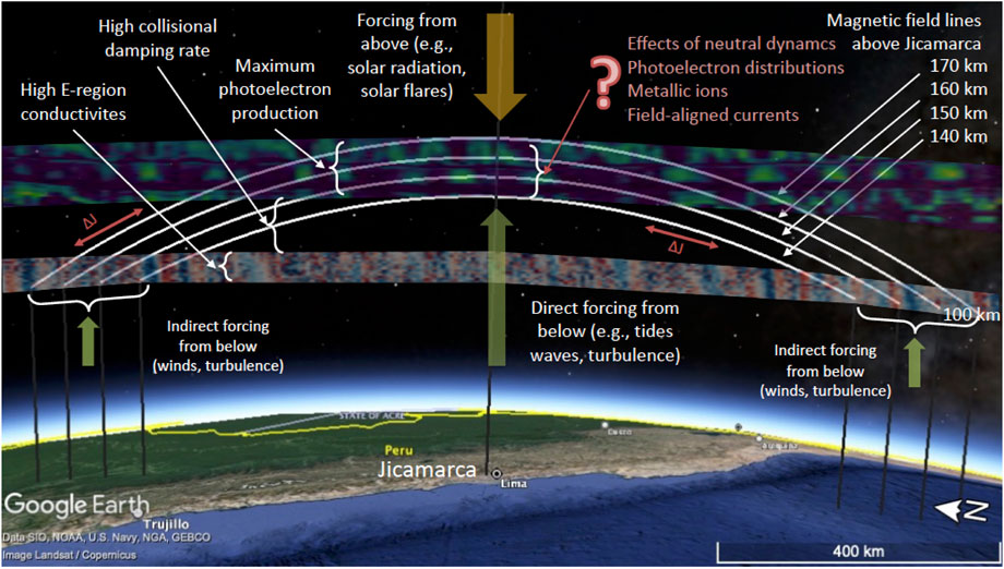
FIGURE 14. North-South sketch of 150-km geometry over Jicamarca. Magnetic field lines connecting altitudes of 140,150, 160, 170 km over Jicamarca to 100 km to the north and south, are indicated. The highly conducting daytime E region and the 150-km region are shaded with different patterns. Text in red indicate potentially missing parameters to understand remaining features of 150-km echoes (adapted from Reyes, 2017, Figure 5.15).

Currently, the UHI theory and EPPIC simulations with photolectrons explain two-thirds of the listed riddles in Table 1 (18 out of 27). Significant progress has definitely been accomplished in recent years.

As discussed in Longley et al. (2020), a few other riddles could be explained by the UHI theory if better background information is provided. For example, we expect that higher resolution WACCM-X could resolve short-time scale N_e variability and therefore the minute scale variability on 150-km echoes (see, e.g., Figure 10). A better representation of the photoelectron distribution, including its altitude and time variability with relatively high resolution (e.g., a few hundred meters and a few minutes), could help to explain the upper boundary (Obs06) and perhaps the narrow forbidden regions (Obs09). Recall, that an ad hoc distribution that is constant in altitude and time was used in Figure 13E. Unfortunately, measurements of photoelectron distributions are scarce. In addition, their actual peaks (and wavelengths) are not only a function of solar radiation but also of atmospheric chemistry and transport (e.g., Varney et al., 2012, and references therein).

One major question remains: How are the low frequency ion waves detected by radars generated? The current UHI theory does not explain the conversion of electron scale waves to the observed ion scale waves. As suggested by Oppenheim and Dimant (2016), the enhanced electron waves appears to couple to ion-acoustic waves non-linearly. Adding weak turbulence theory (e.g., Nicholson, 1983; Forme, 1999) to the UHI theory might help to explain this mode conversion. However, analytical calculations of the connection between UHI and ion waves may prove so difficult that only computational analyses will yield any results.

Besides the natural curiosity to understand the echoes, these echoes represent an observational window to explore the poorly known LLVR (see Section 2). Their Doppler shifts have contributed to a number of aeronomy studies by providing measurements of the F-region mean vertical drifts on a long-term basis to develop empirical models (e.g., Alken, 2009), or to study selected events like ionospheric effects during sudden stratospheric warmings (e.g., Chau et al., 2010a; Patra et al., 2014). Furthermore, 150-km drifts have been used to train and validate neural networks to estimate vertical drifts from magnetometer data (e.g., Anderson et al., 2006; Chaitanya and Patra, 2020),

Solving the remaining riddles could allow the use of the echoes to diagnose other LLVR parameters. For example, (a) high resolution N_e measurements from the wide forbidden gaps, (b) plasma temperatures from oblique NEIS spectra, (c) neutral wind forcing from the temporal evolution of the gaps and the echo structures.

9.2 On the unsolved riddles

From all the unsolved riddles, we consider that the three most important questions still unsolved are: (a) how is the enhancement of NEIS echoes modulated or suppressed (Obs04, Obs11), (b) what are the physics behind FAIs (type B) (Obs19, Obs23), and (c) what is the frequency dependence of NEIS and FAI echoes (Obs24). We believe that solving these three questions, might help to understand the remaining riddles (e.g., zonal asymmetry (Obs15) and solar variability (Obs23) of type B echoes).

Previously, Chau and Kudeki (2013) suggested that the modulator and suppressant of 150-km enhancements might be due to photoelectrons and field-aligned currents. The photoelectron distributions have been shown to be important, but neither the EPPIC simulations nor the UHI theory have included the effects of field-aligned currents. These currents could be the results of complex neutral dynamics acting in the region along B lines.

The UHI theory does not explain the existence of perpendicular-only echoes (type B) since inverse Landau and cyclotron damping cannot occur strictly perpendicular to the magnetic field. However there must be some common governing physics between echoes, given that they share many features (e.g., forbidden regions, necklace shape, daytime, etc.). FAI echoes might be initially NEIS echoes that have gone unstable as the pole describing the equilibrium spectrum of NEIS crosses over from the stable side of the complex frequency plane into the unstable one. This transition cannot be explained by the UHI mechanism, and likely relies on some localized chemistry (e.g., metallic ions), that in turn is the result of neutral dynamics (e.g., tides), similar to the case of sporadic E.

The third major unsolved question, i.e., frequency dependence, might be answered, at least for the NEIS echoes, by improving the EPPIC simulations as well as the UHI theory. In the case of EPPIC simulations higher resolution, more accurate photoelectron distributions and more realistic collisions should help characterize the NEIS at the observed (and not observed) wavelengths. Longley et al. (2020), suggested that incorporating weak-turbulence theory (non-linear terms) to the UHI theory might also help to understand the frequency dependence of NEIs while explaining how the electron modes excited by the UHI convert to the observed ion modes.

9.3 Suggested future observations

To solve all three questions a combination of new observations as well as new developments in simulations and theory are needed. Some qualitative suggestions for simulations and theory improvements have been mentioned above.

In the case of new measurements, here we list some challenging suggestions:

• Multi-frequency and multi-beam along B collocated observations would help to quantify NEIS and FAI echoes occurrence, their relation to type A and type B, and their frequency dependence. These observations could be realized at JRO, Gadanki and perhaps the proposed equatorial MU radar (e.g., Yamamoto et al., 2014), given their sensitivity and beam-pointing capabilities.

• High sensitive ion-line and plasma-line measurements at higher frequencies at ALTAIR. As mentioned above current incoherent scatter measurements of the daytime valley region over ALTAIR have not reported any indication of 150-km echoes (e.g., Kudeki et al., 2006). High sensitive experiments, e.g., maximizing duty cycle and staying at a fix angle for a longer time, should be conducted to confirm the absence or present of 150-km echoes. Even if the echoes are not observed, plasma-line experiments should reveal enhanced plasma lines in the 150-km region in accordance to the existing UHI theory. These experiments might require the use of parallel acquisition system with a relative wide band (±∼5 MHz).

• Daytime lidar measurements covering the LLVR altitudes. High sensitive resonance lidars have been shown to sample these altitudes, at least at night over different latitudes (e.g., Chu et al., 2021, and references therein). Since ground-based lidars require clear-sky conditions, any location at low latitudes would be good, but collocated with a high-power large-aperture radar would be better.

• In situ measurements of electron densities be s, electric fields, currents, and photoelectron distributions would contribute to solve the remaining riddles as well as to verify or challenge the existing theories. They could be performed locally via dedicated rocket campaigns at low latitudes, preferably around a high-power large-aperture radar, or globally on board very low Earth orbiting satellites (e.g., Sarris et al., 2020). Previous LLVR rocket measurements have not shown signatures typically associated to FAIs, however knowing that FAIs do not occur as frequent as NEIS, future observations should be focused on identify NEIS signatures. These considerations are relevant for the recent white paper related to a future rocket campaign under the magnetic equator, that includes research of 150-km echoes (Space-Science-Community, 2018).

• High resolution temporal winds at lower ionospheric altitudes (i.e., 90–120 km) connecting to LLVR altitudes, both north and south, would be needed to understand the observed N_e variability and possibly to characterize field-aligned currents. Ground-based measurements are being pursued with multistatic specular meteor radars (e.g., Chau et al., 2021) but only up to 100–105 km altitude. Satellite measurements, like those from ICON/MIGHTI (e.g., Englert et al., 2017; Harding et al., 2021), could be a good complement if they are routinely made over JRO and with a processing that allows strong horizontal wind shears.

• Three-dimensional radar imaging measurements of 150-km echoes at JRO. Initial 2D imaging experiments have shown that 150-km echoes present kilometer-scale structures in the east-west direction (i.e., transverse to B. Given the modularity of JRO’s main array and the wide SNR range of 150-km echoes, MIMO (Multiple-Input, multiple-output) techniques can help implementing 3D radar imaging with unprecedented resolution (e.g., Urco et al., 2018, 2019). We expect these measurements also to contribute to the separation of NEIS and FAIs and possibly understand their spatial behavior and evolution.

• New and improved measurements of 150-km echoes at other longitudes with less sensitive systems. Less sensitive systems like the 30-MHz systems at Sao Luis and Gadanki (e.g., Rodrigues et al., 2011; Patra et al., 2018) might contribute to study the longitudinal dependence of the echoes. From the UHI theory, a longitudinal dependence is expected given the longitudinal dependence of B (e.g., Alken et al., 2021). For example, the separation between wide gaps should be larger over Gadanki than Jicamarca for the same N_e profile, given Gadanki’s ∼66% larger |B|. The Doppler shifts from these systems will also contribute to the understanding of the longitudinal behavior of other low-latitude aeronomy processes (e.g., Kelley et al., 2007; Stolle and Liu, 2014; Yamazaki et al., 2017).

A full understanding of daytime LLVR echoes is far from being achieved. Their complete knowledge may well represent the last unexplored Frontier in the theory of fluctuations in a plasma teetering at the edge of thermal equilibrium (Chau and Kudeki, 2013).

Author contributions

JC led the team, structured the paper and wrote the first drafts. All authors participated in the discussions leading to this review paper as part of the ISSI team meetings, and contributed to different parts of the text.

Funding

HL acknowledges support from JSPS KAKENHI grants 18H01270, 17KK0095, and JRPs-LEAD with DFG (JPJSJPR 20181602. The Jicamarca Radio Observatory is a facility of the Instituto Geofísico del Perú operated with support from NSF award AGS-1732209 through an agreement with Cornell University. This material is based upon work supported by the National Center for Atmospheric Research, which is a major facility sponsored by the US National Science Foundation under Cooperative Agreement 1852977. JLC and CS acknowledge support by the Deutsche Forschungsgemeinschaft under SPP 1788 (DynamicEarth).

Acknowledgments

JC partially worked on this paper at Kyushu University, Japan during a guest researcher stay funded by NICT (National Institute of Information and Communications Technology, Japan). We thank the Jicamarca staff for their work in making possible the radar observations presented in this paper. Specially thanks to the International Space Science Institute for facilitating discussions related to this work as part of the International Team project #426 (“An Exploration of the Valley Region in the Low Latitude Ionosphere: Response to Forcing from Below and Above and Relevance to Space Weather”).

Conflict of interest

The authors declare that the research was conducted in the absence of any commercial or financial relationships that could be construed as a potential conflict of interest.

Publisher’s note

All claims expressed in this article are solely those of the authors and do not necessarily represent those of their affiliated organizations, or those of the publisher, the editors and the reviewers. Any product that may be evaluated in this article, or claim that may be made by its manufacturer, is not guaranteed or endorsed by the publisher.

References

Alken, P. (2009). A quiet time empirical model of equatorial vertical plasma drift in the Peruvian sector based on 150 km echoes. J. Geophys. Res. 114, 1–6. doi:10.1029/2008JA013751
Alken, P., Thébault, E., Beggan, C. D., Amit, H., Aubert, J., Baerenzung, J., et al. (2021). International geomagnetic reference field: The thirteenth generation. Earth, Planets Space 73, 49. doi:10.1186/s40623-020-01288-x
Anderson, D., Anghel, A., Chau, J. L., and Yumoto, K. (2006). Global, low-latitude, vertical E × B drift velocities inferred from daytime magnetometer observations. Space weather. 4. doi:10.1029/2005SW000193
Anderson, D., Anghel, A., Chau, J., and Veliz, O. (2004). Daytime vertical E × B drift velocities inferred from ground-based magnetometer observations at low latitudes. Space weather. 2. doi:10.1029/2004sw000095
Aponte, N., Woodman, R. F., Swartz, W. E., and Farley, D. T. (1997). Measuring ionospheric densities, temperatures, and drift velocities simultaneously at Jicamarca. Geophys. Res. Lett. 24, 2941–2944. doi:10.1029/97GL02898
Balsley, B. B. (1964). Evidence of a stratified echoing region at 150 kilometers in the vicinity of the magnetic equator during daylight hours. J. Geophys. Res. 69, 1925–1930. doi:10.1029/jz069i009p01925
Balsley, B. B., and Farley, D. T. (1971). Radar studies of the equatorial electrojet at three frequencies. J. Geophys. Res. 76, 8341–8351. doi:10.1029/JA076i034p08341
Basu, B., Chang, T., and Jasperse, J. R. (1982). Electrostatic plasma instabilities in the daytime lower ionosphere. Geophys. Res. Lett. 9, 68–71. doi:10.1029/GL009i001p00068
Blanc, E., Mercandalli, B., and Houngninou, E. (1996). Kilometric irregularities in the E and F regions of the daytime equatorial ionosphere observed by a high resolution HF radar. Geophys. Res. Lett. 23, 645–648. doi:10.1029/96GL00415
Campbell-Brown, M. D. (2019). Solar cycle variation in radar meteor rates. Mon. Notices R. Astronomical Soc. 485, 4446–4453. doi:10.1093/mnras/stz697
Chaitanya, P. P., and Patra, A. K. (2020). A neural network-based model for daytime vertical E× B drift in the Indian sector. J. Geophys. Res. Space Phys. 125, 1–11. doi:10.1029/2020JA027832
Chau, J. L., Aponte, N. A., Cabassa, E., Sulzer, M. P., Goncharenko, L. P., and González, S. A. (2010a). Quiet time ionospheric variability over Arecibo during sudden stratospheric warming events. J. Geophys. Res. 115, 1–8. doi:10.1029/2010JA015378
Chau, J. L., and Hysell, D. L. (2004). High altitude large-scale plasma waves in the equatorial electrojet at twilight. Ann. Geophys. 22, 4071–4076. doi:10.5194/angeo-22-4071-2004
Chau, J. L., and Kudeki, E. (2013). Discovery of two distinct types of equatorial 150 km radar echoes. Geophys. Res. Lett. 40, 4509–4514. doi:10.1002/grl.50893
Chau, J. L., and Kudeki, E. (2006a). First E- and D-region incoherent scatter spectra observed over Jicamarca. Ann. Geophys. 24, 1295–1303. doi:10.5194/angeo-24-1295-2006
Chau, J. L., and Kudeki, E. (2006b). Statistics of 150-km echoes over Jicamarca based on low-power VHF observations. Ann. Geophys. 24, 1305–1310. doi:10.5194/angeo-24-1305-2006
Chau, J. L., Milla, M. A., and Kudeki, E. (2010b). “Multi-frequency radar studies of the equatorial 150 km region,” in Proceedings of the twelfth workshop on technical and scientific aspects of MST radar, 165–168.
Chau, J. L. (2004). Unexpected spectral characteristics of VHF radar signals from 150-km region over Jicamarca. Geophys. Res. Lett. 31, 1–4. doi:10.1029/2004GL021620
Chau, J. L., Urco, J. M., Vierinen, J., Harding, B. J., Clahsen, M., Pfeffer, N., et al. (2021). Multistatic specular meteor radar network in Peru: System description and initial results. Earth Space Sci. 8, e01293. doi:10.1029/2020EA001293
Chau, J. L., and Woodman, R. F. (2005). D- and E-region incoherent scatter radar density measurements over Jicamarca. J. Geophys. Res. 110, A12314. doi:10.1029/2005JA011438
Chau, J. L., and Woodman, R. F. (2004a). Daytime vertical and zonal velocities from 150-km echoes: Their relevance to F-region dynamics. Geophys. Res. Lett. 31, 15–18. doi:10.1029/2004GL020800
Chau, J. L., Woodman, R. F., Milla, M. A., and Kudeki, E. (2009). Naturally enhanced ion-line spectra around the equatorial 150-km region. Ann. Geophys. 27, 933–942. doi:10.5194/angeo-27-933-2009
Chau, J. L., and Woodman, R. F. (2004b). Observations of meteor-head echoes using the Jicamarca 50 MHz radar in interferometer mode. Atmos. Chem. Phys. 4, 511–521. doi:10.5194/acp-4-511-2004
Choudhary, R. K., St.-Maurice, J. P., and Mahajan, K. K. (2004). Observation of coherent echoes with narrow spectra near 150 km altitude during daytime away from the dip equator. Geophys. Res. Lett. 31, L19801–L19805. doi:10.1029/2004GL020299
Christakis, N., Haldoupis, C., Zhou, Q., and Meek, C. (2009). Seasonal variability and descent of mid-latitude sporadic E layers at Arecibo. Ann. Geophys. 27, 923–931. doi:10.5194/angeo-27-923-2009
Chu, X., Chen, Y., Cullens, C. Y., Yu, Z., Xu, Z., Zhang, S.-R., et al. (2021). Mid-latitude thermosphere-ionosphere Na (TINa) layers observed with high-sensitivity Na Doppler lidar over boulder (40.13°N, 105.24°W). Geophys. Res. Lett. 48, e2021GL093729. doi:10.1029/2021GL093729
De Paula, E. R., and Hysell, D. L. (2004). The São Luís 30 MHz coherent scatter ionospheric radar: System description and initial results. Radio Sci. 39, 178–188. doi:10.1029/2003rs002914
Englert, C. R., Harlander, J. M., Brown, C. M., Marr, K. D., Miller, I. J., Stump, J. E., et al. (2017). Michelson interferometer for global high-resolution thermospheric imaging (mighti): Instrument design and calibration. Space Sci. Rev. 212, 553–584. doi:10.1007/s11214-017-0358-4
Farley, D. T. (2009). The equatorial E-region and its plasma instabilities: A tutorial. Ann. Geophys. 27, 1509–1520. doi:10.5194/angeo-27-1509-2009
Fawcett, C. (1999). An investigation of equatorial 150-km irregularities. Ph.D. Thesis. University of Illinois at Urbana-Champaign.
Fontaine, D., and Forme, F. (1995). Ionospheric small-scale structures and turbulence inferred from eiscat observations: A review. J. geomagnetism Geoelectr. 47, 869–878. doi:10.5636/jgg.47.869
Forme, F. R. (1999). Parametric decay of beam-driven Langmuir wave and enhanced ion-acoustic fluctuations in the ionosphere: A weak turbulence approach. Ann. Geophys. 17, 1172–1181. doi:10.1007/s00585-999-1172-4
Fukao, S., Tsuda, T., Sato, T., Kato, S., Wakasugi, K., and Makihira, T. (1985). The MU radar with an active phased array system, 2. In-house equipment. Radio Sci. 20, 1169–1176. doi:10.1029/RS020i006p01169
Harding, B. J., Chau, J. L., He, M., Englert, C. R., Harlander, J. M., Marr, K. D., et al. (2021). Validation of ICON-MIGHTI thermospheric wind observations: 2. Green-line comparisons to specular meteor radars. J. Geophys. Res. Space Phys. 126, e2020JA028947–12. doi:10.1029/2020JA028947
Hysell, D. L., and Burcham, J. D. (2002). Long term studies of equatorial spread F using the JULIA radar at Jicamarca. J. Atmos. Solar-Terrestrial Phys. 64, 1531–1543. doi:10.1016/S1364-6826(02)00091-3
Hysell, D. L., Fritts, D. C., Laughman, B., and Chau, J. L. (2017). Gravity wave-induced ionospheric irregularities in the postsunset equatorial Valley Region. J. Geophys. Res. Space Phys. 122 (579–11), 11590. doi:10.1002/2017JA024514
Hysell, D. L., Larsen, M. F., and Woodman, R. F. (1997). JULIA radar studies of electric fields in the equatorial electrojet. Geophys. Res. Lett. 24, 1687–1690. doi:10.1029/97GL00373
Hysell, D. L., Milla, M. A., and Vierinen, J. (2016). A multistatic HF beacon network for ionospheric specification in the Peruvian sector. Radio Sci. 51, 392–401. doi:10.1002/2016RS005951
Hysell, D. L. (2022). Planned science and scientific discovery in equatorial aeronomy. Front. Astronomy Space Sci. 9, 1–7. doi:10.3389/fspas.2022.883050
Immel, T. J., England, S. L., Mende, S. B., Heelis, R. A., Englert, C. R., Edelstein, J., et al. (2018). The ionospheric connection explorer mission: Mission goals and design. Space Sci. Rev. 214, 13–36. doi:10.1007/s11214-017-0449-2
Janches, D., Heinselman, C. J., Chau, J. L., Chandran, A., and Woodman, R. (2006). Modeling the global micrometeor input function in the upper atmosphere observed by high power and large aperture radars. J. Geophys. Res. Space Phys. 111, A07317. doi:10.1029/2006JA011628
Jasperse, J. R., Basu, B., Retterer, J. M., Decker, D. T., and Chang, T. (1995). High frequency electrostatic plasma instabilities and turbulence layers in the lower ionosphere. American Geophysical Union (AGU, 77–94. doi:10.1029/GM086p0077
Kelley, M. C., Nicolls, M. J., Anderson, D., Anghel, A., Chau, J. L., Sekar, R., et al. (2007). Multi-longitude case studies comparing the interplanetary and equatorial ionospheric electric fields using an empirical model. J. Atmos. Solar-Terrestrial Phys. 69, 1174–1181. doi:10.1016/j.jastp.2006.08.014
Kelley, M. C. (2009). The Earth’s ionosphere: Plasma physics and electrodynamics. San Diego, Calif: Academic.
Kontar, E. P., and Pécseli, H. L. (2005). Nonlinear wave interactions as a model for naturally enhanced ion acoustic lines in the ionosphere. Geophys. Res. Lett. 32, L05110. doi:10.1029/2004GL022182
Kudeki, E., Fawcett, C. D., Ecklund, W. L., Johnston, P. E., and Franke, S. J. (1998). Equatorial 150-km irregularities observed at Pohnpei. Geophys. Res. Lett. 25, 4079–4082. doi:10.1029/1998GL900069
Kudeki, E., and Fawcett, C. D. (1993). High resolution observations of 150 km echoes at Jicamarca. Geophys. Res. Lett. 20, 1987–1990. doi:10.1029/93GL01256
Kudeki, E., Milla, M., Friedrich, M., Lehmacher, G., and Sponseller, D. (2006). ALTAIR incoherent scatter observations of the equatorial daytime ionosphere. Geophys. Res. Lett. 33, 081088–L8115. doi:10.1029/2005GL025180
Kudeki, E., and Milla, M. (2012). “Incoherent scatter radar - spectral signal model and ionospheric applications,” in Doppler radar observations - weather radar, wind profiler, ionospheric radar, and other advanced applications. Editors J. Bech, and J. L. Chau (Intech), 377–408. doi:10.5772/39010
Kudeki, E., and Milla, M. (2006). Incoherent scatter spectrum theory for modes propagating perpendicular to the geomagnetic field. J. Geophys. Res. Space Phys. 111, A06306. doi:10.1029/2005JA011546
Latteck, R., Singer, W., Rapp, M., Vandepeer, B., Renkwitz, T., Zecha, M., et al. (2012). Maarsy: The new MST radar on Andøya-System description and first results. Radio Sci. 47, RS1006. doi:10.1029/2011RS004775
Lee, J., Doering, J., Potemra, T., and Brace, L. (1980). Measurements of the ambient photoelectron spectrum from atmosphere explorer: Ii. ae-e measurements from 300 to 1000 km during solar minimum conditions. Planet. Space Sci. 28, 973–996. doi:10.1016/0032-0633(80)90059-8
Lehmacher, G. A., Wu, H., Kudeki, E., Reyes, P. M., Hysell, D. L., and Milla, M. (2020). Height variation of gaps in 150-km echoes and whole atmosphere community climate model electron densities suggest link to upper hybrid resonance. J. Geophys. Res. Space Phys. 125, 1–11. doi:10.1029/2019JA027204
Li, G., Ning, B., Patra, A. K., Abdu, M. A., Chen, J., Liu, L., et al. (2013). On the linkage of daytime 150 km echoes and abnormal intermediate layer traces over Sanya. J. Geophys. Res. Space Phys. 118, 7262–7267. doi:10.1002/2013JA019462
Longley, W. J., Oppenheim, M. M., Pedatella, N. M., and Dimant, Y. S. (2020). The photoelectron-driven upper hybrid instability as the cause of 150-km echoes. Geophys. Res. Lett. 47, 1–10. doi:10.1029/2020GL087391
Longley, W. J., Vierinen, J., Sulzer, M. P., Varney, R. H., Erickson, P. J., and Perillat, P. (2021). An explanation for Arecibo plasma line power striations. J. Geophys. Res. Space Phys. 126. doi:10.1029/2020JA028734
Lu, F., Farley, D. T., and Swartz, W. E. (2008). Spread in aspect angles of equatorial E region irregularities. J. Geophys. Res. Space Phys. 113. doi:10.1029/2008JA013018
Malhotra, A., Mathews, J. D., and Urbina, J. (2007). Multi-static, common volume radar observations of meteors at Jicamarca. Geophys. Res. Lett. 34, L24103. doi:10.1029/2007GL032104
Matzka, J., Stolle, C., Yamazaki, Y., Bronkalla, O., and Morschhauser, A. (2021). The geomagnetic kp index and derived indices of geomagnetic activity. Space weather. 19, e2020SW002641. doi:10.1029/2020sw002641
McMahon, W. J., and Heroux, L. J. (1983). The 2- to 5-eV energy spectra of thermospheric photoelectrons: Measurements in apparent conflict with theory. J. Geophys. Res. Space Phys. 88, 9249–9254. doi:10.1029/JA088iA11p09249
Milla, M. A., and Kudeki, E. (2011). Incoherent scatter spectral theories—Part II: Modeling the spectrum for modes propagating perpendicular to ${\bf B}$. IEEE Trans. Geoscience Remote Sens. 49, 329–345. doi:10.1109/tgrs.2010.2057253
Milla, M. A., Kudeki, E., Reyes, P. M., and Chau, J. L. (2013). A multi-beam incoherent scatter radar technique for the estimation of ionospheric electron density and Te/Ti profiles at Jicamarca. J. Atmos. Solar-Terrestrial Phys. 105-106, 214–229. doi:10.1016/j.jastp.2013.06.003
Milla, M., and Kudeki, E. (2006). F-region electron density and Te/Ti measurements using incoherent scatter power data collected at ALTAIR. Ann. Geophys. 24, 1333–1342. doi:10.5194/angeo-24-1333-2006
Oppenheim, M. M., and Dimant, Y. S. (2013). Kinetic simulations of 3-D Farley-Buneman turbulence and anomalous electron heating. J. Geophys. Res. Space Phys. 118, 1306–1318. doi:10.1002/jgra.50196
Oppenheim, M. M., and Dimant, Y. S. (2016). Photoelectron-induced waves: A likely source of 150 km radar echoes and enhanced electron modes. Geophys. Res. Lett. 43, 3637–3644. doi:10.1002/2016GL068179
Patra, A. K., Chaitanya, P. P., Rao, M. D., and Kamaraj, P. (2020a). Common-volume dual-frequency radar observations of 150-km echoes and implications. J. Geophys. Res. Space Phys. 125, 1–7. doi:10.1029/2019JA027317
Patra, A. K., Chaitanya, P. P., Rao, M. D., and Reddy, G. J. (2020b). On the type-A and type-B 150-km radar echoes. J. Geophys. Res. Space Phys. 125, 1–9. doi:10.1029/2020JA028551
Patra, A. K. (2011). Descending ion layer property in the Gadanki radar observations of 150 km echoes and its implication to the echoing phenomenon. J. Geophys. Res. Space Phys. 116, A11322. doi:10.1029/2011JA016805
Patra, A. K., and Pavan Chaitanya, P. (2014). Comparative anatomy of the day- and night-time radar echoes from the 130-170 km region of the low latitude ionosphere. Adv. Space Res. 54, 395–402. doi:10.1016/j.asr.2013.07.046
Patra, A. K., Pavan Chaitanya, P., Durga Rao, M., and Kamaraj, P. (2018). First dual-frequency radar observations of 150-km echoes from Gadanki and implications. Geophys. Res. Lett. 45, 4594–4600. doi:10.1029/2017GL076749
Patra, A. K., Pavan Chaitanya, P., Sripathi, S., and Alex, S. (2014). Ionospheric variability over Indian low latitude linked with the 2009 sudden stratospheric warming. J. Geophys. Res. Space Phys. 119, 4044–4061. doi:10.1002/2014JA019847
Patra, A. K., Pavan Chaitanya, P., St.-Maurice, J. P., Otsuka, Y., Yokoyama, T., and Yamamoto, M. (2017). The solar flux dependence of ionospheric 150 km radar echoes and implications. Geophys. Res. Lett. 44, 11,257–11,264. doi:10.1002/2017GL074678
Patra, A. K., Pavan Chaitanya, P., and Tiwari, D. (2011). Characteristics of 150 km echoes linked with solar eclipse and their implications to the echoing phenomenon. J. Geophys. Res. Space Phys. 116, 1–9. doi:10.1029/2010ja016258
Patra, A. K., and Pavan Chaitanya, P. (2016). Unexpected characteristics of the 150 km echoes observed over Gadanki and their implications. Geophys. Res. Lett. 43, 11,129–11,136. doi:10.1002/2016GL071519
Patra, A. K., and Rao, N. V. (2006). Radar observations of daytime 150-km echoes from outside the equatorial electrojet belt over Gadanki. Geophys. Res. Lett. 33, L03104. doi:10.1029/2005GL024564
Patra, A. K., Yokoyama, T., Otsuka, Y., and Yamamoto, M. (2008). Daytime 150-km echoes observed with the equatorial atmosphere radar in Indonesia: First results. Geophys. Res. Lett. 35, L06101. doi:10.1029/2007GL033130
Pavan Chaitanya, P., Patra, A. K., Otsuka, Y., Yokoyama, T., and Yamamoto, M. (2018). On the solstice maxima and azimuth-dependent characteristics of the 150-km echoes observed using the equatorial atmosphere radar. J. Geophys. Res. Space Phys. 123, 6752–6759. doi:10.1029/2018JA025491
Pedatella, N. M., Chau, J. L., Vierinen, J., Qian, L., Reyes, P., Kudeki, E., et al. (2019). Solar flare effects on 150-km echoes observed over Jicamarca: WACCM-X simulations. Geophys. Res. Lett. 165, 10951–10958. doi:10.1029/2019gl084790
Prakash, S., Gupta, S. P., and Subbaraya, B. H. (1969). Irregularities in the equatorial E region over thumba. Radio Sci. 4, 791–796. doi:10.1029/RS004i009p00791
Reyes, P. M., Kudeki, E., Lehmacher, G. A., Chau, J. L., and Milla, M. A. (2020). VIPIR and 50 MHz radar studies of gravity wave signatures in 150-km echoes observed at Jicamarca. J. Geophys. Res. Space Phys. 125. doi:10.1029/2019JA027535
Reyes, P. M. (2012). Solar flare effects observed over Jicamarca during MST-ISR experiments. Master of science. University of Illinois Urbana-Champaign.
Reyes, P. M. (2017). “Study of waves observed,” in The equatorial ionospheric Valley Region using Jicamarca ISR and VIPIR ionosonde (University of Illinois at Urbana-Champaign) Ph.D. Thesis.
Rietveld, M., Collis, P., and St.-Maurice, J.-P. (1991). Naturally enhanced ion acoustic waves in the auroral ionosphere observed with the EISCAT 933-MHz radar. J. Geophys. Res. Space Phys. 96, 19291–19305. doi:10.1029/91ja01188
Rodrigues, F. S., De Paula, E. R., and Chau, J. L. (2011). On the characteristics of 150-km echoes observed in the Brazilian longitude sector by the 30 MHz São Luís radar. Ann. Geophys. 29, 1905–1916. doi:10.5194/angeo-29-1905-2011
Røyrvik, O. (1982). Drift and aspect sensitivity of scattering irregularities in the upper equatorial E region. J. Geophys. Res. 87, 8338. doi:10.1029/ja087ia10p08338
Røyrvik, O., and Miller, K. L. (1981). Nonthermal scattering of radio waves near 150 km above Jicamarca, Peru. J. Geophys. Res. 86, 180. doi:10.1029/ja086ia01p00180
Sarris, T. E., Talaat, E. R., Palmroth, M., Dandouras, I., Armandillo, E., Kervalishvili, G., et al. (2020). Daedalus: A low-flying spacecraft for in situ exploration of the lower thermosphere–ionosphere. Geoscientific Instrum. Methods Data Syst. 9, 153–191. doi:10.5194/gi-9-153-2020
Schunk, R., and Nagy, A. (2009). Ionospheres: Physics, plasma physics, and chemistry. Cambridge University Press.
Shepherd, G. G., Thuillier, G., Cho, Y.-M., Duboin, M.-L., Evans, W. F. J., Gault, W. A., et al. (2012). The wind imaging interferometer (windii) on the upper atmosphere research satellite: A 20 year perspective. Rev. Geophys. 50. doi:10.1029/2012RG000390
Smith, L. G., and Royrvik, O. (1985). Electron-density irregularities in the day-time equatorial ionosphere. J. Atmos. Terr. Phys. 47, 813–824. doi:10.1016/0021-9169(85)90056-X
Space-Science-Community (2018). White paper: A nasa sounding rocket campaign in Peru – unprecedented, Preeminent Science at a Unique Observing Site.
Stolle, C., and Liu, H. (2014). Low-latitude ionosphere and thermosphere. American Geophysical Union AGU, 259–272. chap. 21. doi:10.1002/9781118704417.ch21
Stolle, C., Manoj, C., Lühr, H., Maus, S., and Alken, P. (2008). Estimating the daytime equatorial ionization anomaly strength from electric field proxies. J. Geophys. Res. Space Phys. 113. doi:10.1029/2007JA012781
Sulzer, M. P., and González, S. (1999). The effect of electron Coulomb collisions on the incoherent scatter spectrum in the F region at Jicamarca. J. Geophys. Res. Space Phys. 104, 22535–22551. doi:10.1029/1999ja900288
Tepley, C. A., and Mathews, J. D. (1985). An incoherent scatter radar measurement of the average ion mass and temperature of a nighttime sporadic layer. J. Geophys. Res. Space Phys. 90, 3517–3519. doi:10.1029/JA090iA04p03517
Tsunoda, R. T., and Ecklund, W. L. (2004). On a summer maximum in the occurrence frequency of 150 km (F1 radar echoes over Pohnpei. Geophys. Res. Lett. 31, 2–5. doi:10.1029/2003gl018704
Tsunoda, R. T., and Ecklund, W. L. (2000). On the nature of 150-km radar echoes over the magnetic dip equator. Geophys. Res. Lett. 27, 657–660. doi:10.1029/1999GL003689
Tsunoda, R. T., and Ecklund, W. L. (2008). On the sheet-like nature of 150 km (F1) radar echoes. Geophys. Res. Lett. 35, L05102. doi:10.1029/2007GL032152
Tsunoda, R. T., and Ecklund, W. L. (2007). On the visibility and zenithal confinement of 150 km (F1) radar echoes. Geophys. Res. Lett. 34, L21102. doi:10.1029/2007GL031276
Tsunoda, R. T. (1994). Enhanced velocities and a shear in daytimeEsqover Kwajalein and their relationship to 150 km echoes over the dip equator. Geophys. Res. Lett. 21, 2741–2744. doi:10.1029/94GL02507
Urco, J. M., Chau, J. L., Milla, M. A., Vierinen, J. P., and Weber, T. (2018). Coherent MIMO to improve aperture synthesis radar imaging of field-aligned irregularities: First results at Jicamarca. IEEE Trans. Geoscience Remote Sens. 56, 2980–2990. doi:10.1109/TGRS.2017.2788425
Urco, J. M., Chau, J. L., Weber, T., and Latteck, R. (2019). Enhancing the spatiotemporal features of polar mesosphere summer echoes using coherent MIMO and radar imaging at MAARSY. Atmos. Meas. Tech. 12, 955–969. doi:10.5194/amt-12-955-2019
Varney, R. H., Swartz, W. E., Hysell, D. L., and Huba, J. D. (2012). Sami2-PE: A model of the ionosphere including multistream interhemispheric photoelectron transport. J. Geophys. Res. Space Phys. 117. doi:10.1029/2011JA017280
Woodman, R. F., and Chau, J. L. (2002). First Jicamarca radar observations of two-stream e region irregularities under daytime counter equatorial electrojet conditions. J. Geophys. Res. Space Phys. 107, SIA 18-1–SIA 18-8. doi:10.1029/2002JA009362
Woodman, R. F. (1971). Inclination of the geomagnetic field measured by an incoherent scatter technique. J. Geophys. Res. 76, 178–184. doi:10.1029/ja076i001p00178
Woodman, R. F. (2004). On a proper electron collision frequency for a Fokker-Planck collision model with Jicamarca applications. J. Atmos. Solar-Terrestrial Phys. 66, 1521–1541. doi:10.1016/j.jastp.2004.07.001
Woodman, R. F. (2009). Spread f – An old equatorial aeronomy problem finally resolved? Ann. Geophys. 27, 1915–1934. doi:10.5194/angeo-27-1915-2009
Yamamoto, M., Hashiguchi, H., Yamamoto, M., and Tsuda, T. (2014). “Equatorial MU radar project,” in 2014 XXXIth URSI general assembly and scientific symposium (URSI GASS), 1. doi:10.1109/URSIGASS.2014.6929772
Yamazaki, Y., Stolle, C., Matzka, J., Siddiqui, T. A., Lühr, H., and Alken, P. (2017). Longitudinal variation of the lunar tide in the equatorial electrojet. J. Geophys. Res. Space Phys. 122 (445–12), 12,445–12,463. doi:10.1002/2017JA024601
Yokoyama, T., Hysell, D. L., Patra, A. K., Otsuka, Y., and Yamamoto, M. (2009). Zonal asymmetry of daytime 150-km echoes observed by Equatorial Atmosphere Radar in Indonesia. Ann. Geophys. 27, 967–974. doi:10.5194/angeo-27-967-2009
Keywords: valley region, upper hybrid instabilities, field-aligned irregularities, photolectrons, kinetic theory, incoherent scatter theory, coherent scatter, ionospheric radars
Citation: Chau JL, Longley WJ, Reyes PM, Pedatella NM, Otsuka Y, Stolle C, Liu H, England SL, Vierinen JP, Milla MA, Hysell DL, Oppenheim MM, Patra A, Lehmacher G and Kudeki E (2023) Solved and unsolved riddles about low-latitude daytime valley region plasma waves and 150-km echoes. Front. Astron. Space Sci. 10:1091319. doi: 10.3389/fspas.2023.1091319
Received: 06 November 2022; Accepted: 15 February 2023;
Published: 27 February 2023.
Edited by:
Jaroslav Chum, Institute of Atmospheric Physics (ASCR), CzechiaReviewed by:
Deepak Karan, University of Colorado Boulder, United StatesJohn Meriwether, New Jersey Institute of Technology, United States
Copyright © 2023 Chau, Longley, Reyes, Pedatella, Otsuka, Stolle, Liu, England, Vierinen, Milla, Hysell, Oppenheim, Patra, Lehmacher and Kudeki. This is an open-access article distributed under the terms of the Creative Commons Attribution License (CC BY). The use, distribution or reproduction in other forums is permitted, provided the original author(s) and the copyright owner(s) are credited and that the original publication in this journal is cited, in accordance with accepted academic practice. No use, distribution or reproduction is permitted which does not comply with these terms.
*Correspondence: J. L. Chau, chau@iap-kborn.de