Energy Expenditure of Dynamic Submaximal Human Plantarflexion Movements: Model Prediction and Validation by in-vivo Magnetic Resonance Spectroscopy

1. Introduction

Musculoskeletal models are important to predict internal forces and muscular energy expenditure, as it is very challenging to measure both in vivo during dynamic movements in humans. Models of muscle contraction dynamics predict forces depending on the length and activity of the muscle tendon unit (MTU) (Winters, 1990; van Soest et al., 1993; Siebert et al., 2003, 2008; Rode et al., 2009; Millard et al., 2013; Haeufle et al., 2014). Models of activation dynamics relate neuronal stimulation to muscle activity (Hatze, 1978; Zajac, 1989; Rockenfeller et al., 2015). Building on these approaches, energy expenditure can be modeled depending on the mechanical and chemical states of the muscles (Umberger et al., 2003; Umberger and Rubenson, 2011; Miller, 2014). However, experimental data to validate such models in humans are rare. Therefore, the aim of this contribution was to perform comprehensive in vivo measurements in human muscles including the acquisition of myoelectric activations and mechanical forces during a defined load as well as determining the corresponding chemical energy turnover changes. These latter changes were used to assess energy supply and to compare it with energy expenditure predicted by a dedicated model.

Validating energy expenditure predicted by muscle models is difficult, because muscles not only produce mechanical work—which can be estimated externally from joint kinematics—but also heat. All energy needed for muscle contraction is provided by adenosine triphosphate (ATP) hydrolysis and can be attributed to three dominating processes: (1) the cross-bridge cycling generating mechanical work, (2) pumping calcium ions from the sarcoplasmic reticulum to the myoplasm, and (3) pumping potassium and sodium ions across the sarcolemma (Barclay, 2015). The latter two processes are associated with the transformation of chemical energy into heat and thus reduce the maximum efficiency of a contraction to generate mechanical work (efficiency = mechanical work/energy expenditure) to about 30%. In addition, the maximum efficiency can be further reduced depending on the activation level of the muscle and on the type of contraction (for review see Woledge et al., 1985; Barclay, 2015). To adequately represent these relations in dynamic movement simulations, models of muscular energy expenditure have been developed based on very precise experiments.

Most previous experiments were performed in isolated muscles, especially in frog muscles (Wilkie, 1968; Homsher et al., 1975; Curtin and Woledge, 1979), as these single preparations enable measurements of heat release during contraction. The use of skinned muscle fibers is particularly suitable, as it further enables direct measurement of cross-bridge dependent ATP turnover based on, e.g., a genetically engineered phosphate-binding protein labeled with a coumarin fluorescent probe (Ferenczi et al., 1995) or by monitoring the oxidation of nicotinamide adenine dinucleotide (NADH, which is linked to ADP formation) using spectrophotometric or fluorimetric methods (Takashi, 1979; Barclay, 2015).

Such experiments provide a good foundation for the development of so-called Hill-type models of muscular energy expenditure of individual muscles in terms of stimulation, activity, force, length, and contraction velocity (Umberger et al., 2003; Bhargava et al., 2004; Lichtwark and Wilson, 2005; Umberger and Rubenson, 2011). Integrated into computer simulations, such muscle models allow to estimate the energy consumption of individual muscles during complex dynamic movements, e.g., during human locomotion (Umberger et al., 2003; Umberger and Rubenson, 2011; Miller et al., 2012; Miller, 2014).

The validation of these advanced simulations requires in vivo measurements of the muscular energy turnover, for example by using the spirometry technique, which enables quantitation of oxygen consumption (inhaled oxygen volume, VO2). However, although being able to identify the locomotion related energy demand changes (Collins et al., 2015), spirometry fails to assess the energy metabolism in individual muscles (Umberger and Rubenson, 2011). A more suitable approach relies on heat measurements in human muscles (Edwards et al., 1975; González-Alonso et al., 2000). However, their application in vivo remains challenging since the following processes have to be taken into account: heat accumulation in muscles, heat removal to the body core mediated by blood circulation and lymph drainage, as well as heat transfer to the skin via convection and conductance (González-Alonso et al., 2000).

On the other hand, dynamic phosphorus magnetic resonance spectroscopy (³¹P-MRS) allows non-invasive, quantitative, localized and simultaneous measurement of different energy metabolites in muscles and thus appears to be a much more favorable technique to obtain appropriate experimental data for the validation of energy turnover models. Besides being able to quantify cell internal phosphate buffer phosphocreatine (PCr) and its intermediate product inorganic phosphate (Pi), ³¹P-MRS also allows measurements of the main energy source adenosine triphosphate (ATP). Acquiring a series of ³¹P-MR spectra during muscle load allows to monitor metabolic processes such as the exercise-induced PCr depletion. During the first seconds of exercise, PCr depletion reflects almost directly the ATP synthesis and immediate ATP demand (Kemp, 2015). Furthermore, the chemical shift of the Pi resonance enables to extract the intra-cellular pH value, because the former is determined by the concentration of free hydrogen ions in the tissue (Heerschap et al., 1999; Rzanny et al., 2016). Therefore, inspecting the load evoked pH changes allows differentiation between alternative ATP synthesis pathways such as alkaline creatine kinase reaction (pH increase) and anaerobic glycolysis (pH decrease). When the pH-increase starts to slow down, the ATP synthesis via glycolysis becomes more dominant. Thus, from the point when the pH reaches its maximum, the ATP demand cannot be estimated anymore based on PCr depletion.

Against this background, the aim of this study was to quantify the ATP turnover rate in the human calf muscle based on PCr depletion of dynamic exercise and use these data to validate a Hill-type model of muscular energy consumption. We hypothesized that the energy expenditure derived from the ³¹P-MRS data matches the energy expenditure predicted by the Hill-type model in a repetitive submaximal exercise for approximately 25 s and will drifting apart when the pH value reaches its maximum. Therefore, we focus on these first 25 s as our validation phase. A model validated by this approach can be used in future studies to predict energy expenditure for sub-maximal dynamic contractions.

2. Experiments

All measurements were conducted in one healthy male subject (age: 36 y., height: 1.94 m, weight: 92 kg, BMI: 25) on the same day. The subject was informed about the aims and risks of the study and gave his written consent before the experiments started. The study was approved by the local ethics committee of the University Hospital of Jena, Germany.

Figure 1 shows the study protocol consisting of three separate experiments. In experiment 1, high resolution MRI scans were performed to obtain the anatomy of the right foot and calf (e.g., muscle volume, internal muscle moment arm). Experiments 2 and 3 were conducted to acquire electromyography (EMG) and ³¹P-MRS data in the M. gastrocnemius medialis (GM) during a defined repetitive plantarflexion exercise. While using the same load regimes, experiments 2 and 3 were performed separately in order to avoid interferences between the EMG and ³¹P-MRS acquisitions.

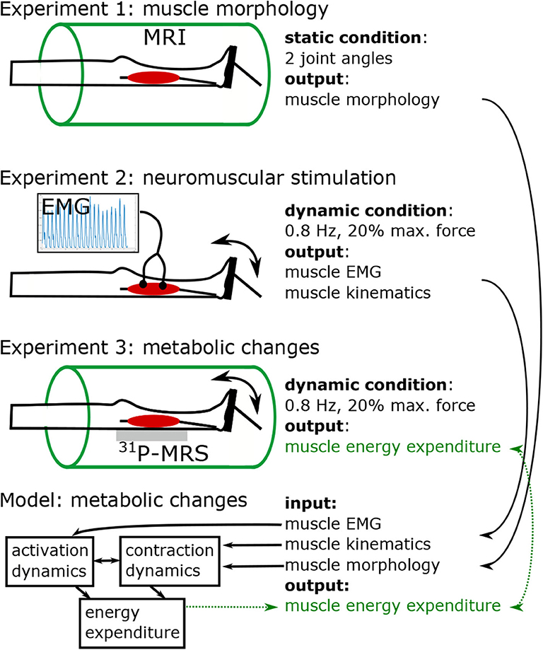
Figure 1. Study design, including three experiments and model based simulation of energy turnover changes in loaded calf muscle. Experiment 1: Structural MRI to determine muscle volume, muscle-tendon-unit length, fiber length, fiber angle, and lever arm in two joint angles (neutral, and extended). Morphological data was used to individualize the leg-foot geometry in the muscle model. Experiments 2 (EMG) and 3 (³¹P-MRS) were performed in a contracting calf muscle at 20% of the single repetition maximum force with 0.8 Hz pedaling cadence. Data from Experiment 2 were used to determine dynamic muscle length (based on recorded joint angle) and myoelectrical stimulations (EMG) during the exercise. The ³¹P-MRS data were used to quantify the ATP turnover and to determine the muscular energy expenditure, which was compared with the output of model based simulations. The model receives input from experiment 1 in terms of muscle parameters and experiment 2 in terms of dynamic muscle length and EMG.

All measurements were performed in supine position with an in-house, MR-compatible pedal ergometer, which is equipped with appropriate sensors and a graphical user interface to monitor the angulation and force magnitudes (Tschiesche et al., 2014; Stutzig et al., 2017). The foot was angulated between 0° (foot sole perpendicular to the shank) and 25° (plantarflexion) and the leg was fixed using a belt attached approximately 3 cm proximal to the patella. Prior to the main exercises, the volunteer performed a standardized warm-up consisting of 10 submaximal isometric plantarflexions. Next, the subject performed one isometric (no joint movement) maximum voluntary contraction at rest angle (later used to normalize EMG) followed by three single repetition maximum contractions (with joint movement) separated by 1 min each (used for determining the submaximal force level for the main experiment).

MR measurements were conducted on a clinical 3 T whole-body MR scanner (Magnetom PRISMA fit; bore size, 60 cm; VE11B, Siemens Healthcare, Erlangen, Germany). Scans were performed using either a flexible phased-array surface coil (Siemens Healthcare, Erlangen, Germany) or a double-tuned (¹H/³¹P) transmit/receive flexible surface coil with an integrated ³¹P-loop (diameter 11 cm, RAPID BioMedical; Rimpar, Germany). The coils were wrapped around the right lower leg.

2.1. Experiment 1 - Determination of Muscle Morphology

To determine geometrical parameters of the M. gastrocnemius medialis, which are needed for the muscle model (see section 3), we collected two high resolution T₁ weighted MRI data sets in two positions (ϕ = 0° neutral ankle position and ϕ = 25° ankle flexion). Each dataset was generated by assembling three, separately acquired and overlapping MRI data volumes covering, first, the upper part of lower leg with the knee joint, second, the middle lower leg part and, third, the lower part of lower leg with the ankle joint and feet. We used a 3D VIBE sequence with an isotropic spatial resolution of 0.8 mm³ (TR/TE = 4.65/2.46 ms, flip angle: 8°, 3 averages, matrix size: 320 × 320, FOV_{AP × FH}: (256 × 256) mm, 160 sagittal slices, 0.8 mm slice thickness, TA: 4 min). The assembling of data sets was performed by using an automatic registration routine available on the analysis console of the MR scanner. The assembled 3D data set was saved as a DICOM image series and manually segmented by using OsiriX MD software (Pixmeo SARL, Bernex, Switzerland). Based on this analysis, muscle volume (V), muscle-tendon-unit length (l_MTU), muscle fiber length (l_{CE, opt}), pennation angle (α), and lever arm (r) were determined for the M. gastrocnemius medialis (see also Table 1 and section 3.1).

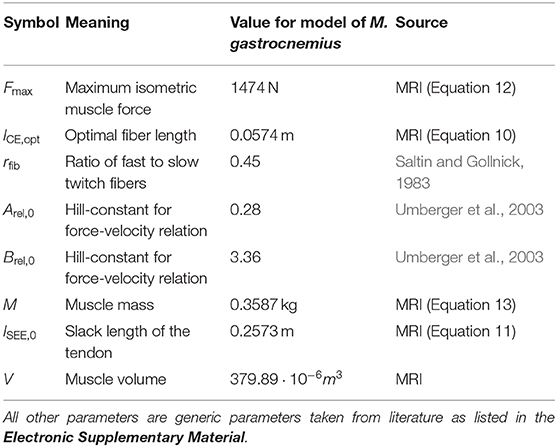
Table 1. Subject specific model parameters.

Figure 2 illustrates the anatomical landmarks (Figures 2A–C), which were identified on MR images to determine the tendon l_SEE and muscle fiber lengths l_CE, as well as a GM surface (Figure 2D), which was manually segmented and used to calculate the muscle volume V. The tendon length l_SEE was determined as a distance between the insertion of the Achilles tendon (Figure 2C) to the most distal GM part landmark (Figure 2B), which was accessed by identifying the first transverse MRI slice containing the GM muscle. The muscle length l_MTU was estimated as a distance between the most distal GM part landmark (Figure 2B) and the landmark indicating the GM origin at the medial condyle of the femur (Figure 2A). The pennation angle α = 27° and the fascicle length l_{CE, opt} = 57 mm were determined based on sagittal plane, solely. Due to the fact that the structures were hard to find in the MR images, we compared our results with studies that examined the architecture of the gastrocnemius medialis using ultrasound (Narici et al., 1996; Arampatzis et al., 2006). The acquired parameters show a good agreement with data reported in literature especially for fiber length. The pennation angle is slightly higher than the data found in the literature. An architectural deviation might be due to compression by the flexible coil which was positioned around the shank in our study.

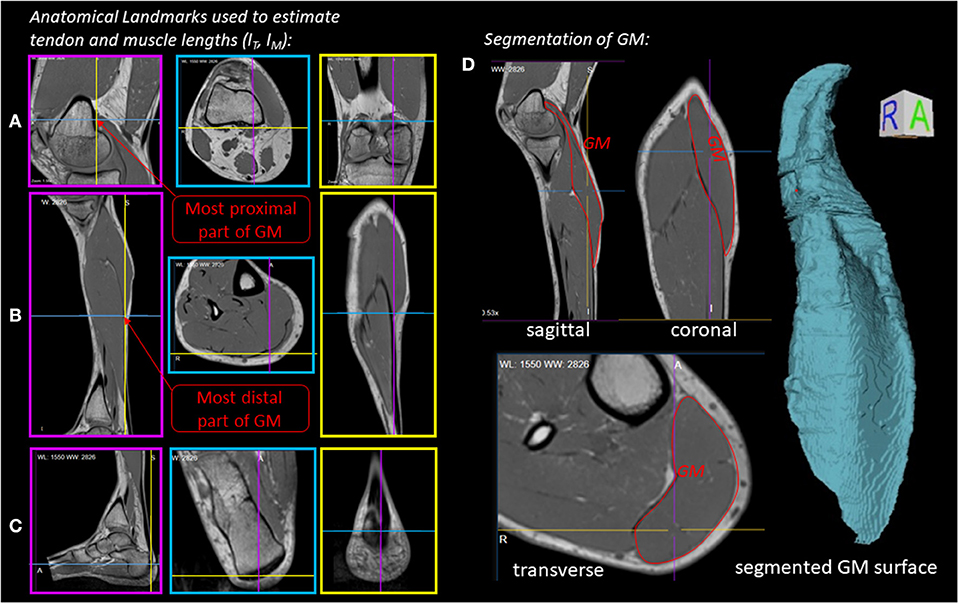
Figure 2. Experiment 1—Determination of muscle morphology: (A–C) Sagittal (magenta boxes), transverse (blue boxes) and coronal (yellow boxes) MRI planes illustrating anatomical landmarks (indicated by line cross-sections), which were identified to determine the tendon (l_SEE) and muscle lengths (l_CE). (D) Manually segmented GM muscle and corresponding GM surface.

2.2. Experiment 2 - Determination of Neuromuscular Stimulation

The dynamic exercises in experiment 2 consisted of dynamic plantarflexion series (3 min exercise + 27 min recovery) at 20% of the mean force level achieved in the three single repetition maxmimum trials. The subject was asked to maintain a pedaling frequency of 0.8 Hz while being assisted by a metronome. In experiment 2, surface EMG and joint angle were recorded to be used as input to the muscle model (Figure 1).

Surface EMG data were recorded using a previously described electrode positioning scheme (Stutzig and Siebert, 2016) and by following the recommendations of Barbero et al. (2012). The skin under the electrodes was shaved, abraded and cleaned with an alcohol solution (according to SENIAM recommendations, Hermens et al., 2000). Two bipolar Ag/AgCl electrodes were affixed with an inter-electrode distance of 20 mm. The data were recorded with a sample rate of 2 kHz, pre-amplified (factor 1000), bandpass filtered (10–500Hz), and rectified by a Biopac MP160 system (Biopac Systems, Goleta, California, USA). The EMG data were normalized to the EMG maximum obtained during the maximum voluntary contraction trial.

2.3. Experiment 3 - Determination of Metabolic Changes

We employed dynamic phosphorus magnetic resonance spectroscopy (³¹P-MRS) to measure the change in phosphocreatine (PCr) concentration ([PCr], the brackets indicate the concentration of PCr), reflecting the ATP concentration change in the muscle. The movements were identical as in experiment 2.

An in-house developed ³¹P-MRS pulse sequence, dubbed MUSCLE (MUlti SliCe Localized Excitation (Moll et al., 2018); TR = 5, 000 ms; flip angle: 50°; acquisition delay between excitation RF pulse and acquisition: 1.3 ms; excitation pulse duration/bandwidth: 1, 600 μs/2.5 kHz), was used to acquire series of 360 single ³¹P-MR spectra in a 16 mm thick slice covering the M. gastrocnemius medialis (see Figure 3 for slice positions). In an entire ³¹P-MR spectra series (see the right chart of Figure 3), 24 spectra were measured during rest (2 min), followed by the acquisition of 36 spectra during load (3 min), and 300 spectra during recovery (25 min). The series was acquired with a temporal resolution of 5 s. Prior to acquiring the dynamic ³¹P-MRS data, a fully recovered resting state spectrum (reference spectrum) was collected with TR of 15 s.

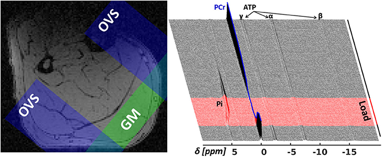
Figure 3. Left: Transverse T₁-weighted gradient-echo image (3D T₁-weighted gradient-echo MRI, TR/TE = 10/6.15 ms) with selected ³¹P-MRS slice in M. gastrocnemius medialis (GM, green area) and outer volume suppression bands (OVS, blue areas) selected to suppress signal contributions from adjacent tissue. Right: “Stack plot” of dynamic ³¹P-MR spectra series from GM muscle. The spectra acquired during the 3 min load phase (red graphs in the right chart) show rapid PCr decrease during the validation phase as well as a subsequent, significant resonance frequency shift of inorganic phosphate (Pi) due to a strong, anaerobic glycolysis related pH decrease. Please note that this paper focuses on the first steep decrease of PCr in the validation phase (t < 25 s).

All MR spectra were corrected for zero- and first-order phase errors, frequency shifts as well as baseline distortions by using an in-house MATLAB script and were quantified with an AMARES routine with prior knowledge for linewidth, frequency and peak shape (Vanhamme et al., 1997) included in the jMRUI 5.2 software (Stefan et al., 2009). Whereas the PCr peak at 0 ppm was fitted as a single Lorentzian line, the α-ATP (at −7.52 ppm) and γ-ATP (−2.48 ppm) doublets and the β-ATP triplet (−16.26 ppm) were quantified with pre-constrained linear combinations of two and three Lorentzian lines, respectively. Absolute PCr concentrations ([PCr]) were determined from the reference spectrum by normalizing the peak intensities (I_PCr) with the γ-ATP intensity (I_γ-ATP) and by assuming a resting state muscle ATP concentration of 8.2 mmol/l ([PCr] = 8.2 mmol/l × I_PCr/I_γ-ATP) (Kemp et al., 2007).

2.4. Analysis of Energy Expenditure in the Validation Phase

The energy demand to maintain muscle performance is met by the breakdown of ATP, which is transferred to the myosin head of the muscle fibers during the cross-bridge cycle with subsequent hydrolysis (Equation 1; Barclay and Weber, 2004). Since ATP depletion is quickly compensated via the creatine kinase reaction (CK; Equation 2), there are usually no ³¹P-MR spectroscopically detectable ATP changes that could be used to assess the energy demand. However, in the validation phase (t < 25 s), the ATP synthesis rate can be derived from the depletion rate of PCr, which is consumed at the same rate as the rate of the ATP synthesis:

Therefore, the energy expenditure dE/dt can be determined from the measured PCr breakdown rate d[PCr]/dt and the enthalpy of ATP hydrolysis △_RH(ATP)

with ${△}_{R}H(ATP)=21kJmo{l}^{-1}$ (Kodama, 1985; see Table 4, for temperature of 38°C). This indicates that an ATP hydrolysis rate of 1 mmol l⁻¹s⁻¹ is associated with a release of 21J reaction heat per liter cell water per second. To calculate the energy released per kilogram of muscle wet weight, we used a conversion factor of $c_{\mathrm{\text{vol}}\to \mathrm{\text{mass}}}=0.68lk{g}^{-1}$ provided by Kemp et al. (2007, Table 1, second row):

By approximating the rate of change of PCr concentration by

the energy release can directly be calculated from the ³¹P-MRS data (with Equation 4)

Please note that this relation only holds in the validation phase (t < 25 s) where the ATP synthesis is dominated by the depletion of PCr.

3. Model

To predict muscular energy expenditure, we combined the following three existing models describing: (a) the contraction dynamics based on a four-element Hill-type muscle model including series elastic damping characteristics (Haeufle et al., 2014), (b) the activation dynamics (Umberger et al., 2003), and (c) the energy consumption (Umberger et al., 2003).

The MTU contraction dynamics is based on a Hill-type muscle model (Haeufle et al., 2014), which considers force-length-velocity characteristics of the fibers (contractile element CE), parallel connective tissue elasticities (parallel elastic element PEE), tendon elasticity (serial elastic element SEE), and tendon damping characteristics (serial damping element SDE). The model has one internal degree of freedom represented by the length of the contractile element l_CE. Thus, the contraction dynamics of the MTU is described by a differential equation

where the fiber contraction velocity (${\stackrel{\cdot }{l}}_{\mathrm{\text{CE}}}$) is a function of the fiber length (l_CE), the length (l_MTU), and contraction velocity of the muscle tendon unit (${\stackrel{\cdot }{l}}_{\mathrm{\text{MTU}}}$) and the muscle fiber activity (a). The model predicts the muscle fiber force F_CE and is described in detail in Haeufle et al. (2014).

The activation dynamics model considers the complex biochemical relation between neuronal stimulation of the muscle, u, and muscle activity a, where 0.001 ≤ a ≤ 1 and 0 ≤ u ≤ 1 are normalized variables. These processes can be approximated by a first order differential equation (He et al., 1991; Umberger et al., 2003)

with different time constants considering faster activation τ_ACT = 58.8 ms than deactivation τ_DEACT = 64.8 ms of muscle fibers (calculated by Equation 4 in Umberger et al., 2003 with %FT = r_fib = 0.45 in accordance to Saltin and Gollnick 1983).

The model for the energy expenditure of the MTU considers the non-linear relation between muscle activation, contraction state, and energy expenditure, as well as the fiber type composition (Umberger et al., 2003). It calculates the total energy rate

as the sum of three components: the activation heat rate and maintenance heat rate ḣ_AM = f_hAM(l_CE, u, a), the shortening-lengthening heat rate ${ḣ}_{\mathrm{\text{SL}}}=f_{\mathrm{\text{hSL}}}({\stackrel{\cdot }{l}}_{\mathrm{\text{CE}}},l_{\mathrm{\text{CE}}},u,a)$, and the mechanical work rate ${ẇ}_{\mathrm{\text{CE}}}=f_{\mathrm{\text{wCE}}}({\stackrel{\cdot }{l}}_{\mathrm{\text{CE}}},F_{\mathrm{\text{CE}}})$. All state variables required to calculate the energy expenditure are provided by the model of the contraction and activation dynamics of the MTU.

All model equations were implemented in Matlab Simulink R2018a (Mathworks Inc.). The model is provided open-source via github (https://github.com/daniel-haeufle/macroscopic-muscle-model) and attached as Electronic Supplementary Material.

3.1. Model Parameters

Most of the parameters of all three model parts were taken from the original sources [contraction dynamics (Haeufle et al., 2014), activation dynamics (He et al., 1991; Umberger et al., 2003), and energy expenditure (Umberger et al., 2003)]. The muscle specific parameters are listed in Table 1 and the complete parameter set is provided with the model in the Electronic Supplementary Material (Haeufle, 2020).

We set the optimal length of the contractile element equal to the fiber length at the pedal rest position

The slack length of the serial elastic element was calculated as

The maximum isometric force F_max was determined based on the muscle volume (V) (Holzbaur et al., 2005) as

with the overall maximum muscle stress σ = 0.25 MPa (Umberger et al., 2003) and pennation angle α = 27°, which was obtained from anatomic MRI data. The mass of the muscle was calculated to be

with the muscle tissue density ρ = 1059.7 kg/m³ (Méndez et al., 1960). We set the fiber type composition (ratio of fast to slow twitch fibers) to r_fib = 0.45, which corresponds to trained distance runners with the mean age of 35 years (Saltin and Gollnick, 1983) matching our subject. This results in Hill parameters according to Umberger et al. (2003) of A_{rel, 0} = 0.1+0.4r_fib = 0.28 and B_{rel, 0} = 12A_{rel, 0} = 3.36.

As the parameters determined from the MRI images are prone to measurement errors, we estimated the effect of variations in these parameters on the calculation of the total energy by means of a Monte Carlo simulation (100 runs). For this, we estimated errors of Δl_{CE, opt}/l_{CE, opt} = 10%, $\Delta l_{\mathrm{\text{MTU}}}(\varphi =0^{\circ })/l_{\mathrm{\text{MTU}}}(\varphi =0^{\circ })=5\%$, and Δα/α = 10%. The mean effect of these variations is indicated by the light-blue area around the simulation results in Figure 5 and appears to be marginal (<1.3%) with respect to the magnitude of the simulated energy expenditure.

3.2. Simulation

The simulation reproduced the experimental conditions of the dynamic plantarflexion movements (experiments 2 and 3). We derived the MTU kinematics l_MTU(t) and ${\stackrel{\cdot }{l}}_{\mathrm{\text{MTU}}}(t)$ from the foot pedal angle ϕ(t) as recorded by the ergometer. We assumed a constant muscle lever arm of r = 0.064 m as determined from the MRI data set (experiment 1). We fitted a tenth-order polynomial to the angle data which allowed to analytically calculate a smooth derivative for ${\stackrel{\cdot }{l}}_{\mathrm{\text{MTU}}}(t)$. For the muscle stimulation signal u(t), we used the rectified and normalized EMG signal measured in experiment 2.

The boundary conditions for the simulation were chosen in accordance with the experimental data. From the initial joint angle ϕ(t = 0) = 3.13° we calculated the initial MTU length as l_{MTU, init} = 0.311 m. The initial muscle activity was a_init = 0.005, corresponding to the initial stimulation u(t = 0) = 0.005 from the normalized EMG signal. This allows to determine the boundary condition for the muscle model's internal degree of freedom, the muscle fiber length l_{CE, init} = 0.052 m: by assuming static force equilibrium at t = 0, all velocity dependent terms in the muscle model vanish and the length of the contractile element can be calculated from the force-length curve of the CE and SEE with the parameters l_{MTU, init} and a_init (see Haeufle et al., 2014 for more details).

The differential equations were solved with ODE23s Simulink built-in variable time step solver with relative tolerance of 1·10⁻⁴.

4. Results

Figure 4A shows a typical PCr evolution for an intense muscle exercise. It starts with a strong PCr depletion during the validation phase (t < 25 s), which levels off approximately after 60 s. The H⁺ consumption accompanying the initial PCr breakdown is indicated by a continuous pH increase from 7.05 to 7.1 (Figure 4B) followed by a strong pH decrease (H⁺ accumulation) in the later exercise phase, which is dominated by anaerobic glycolysis.

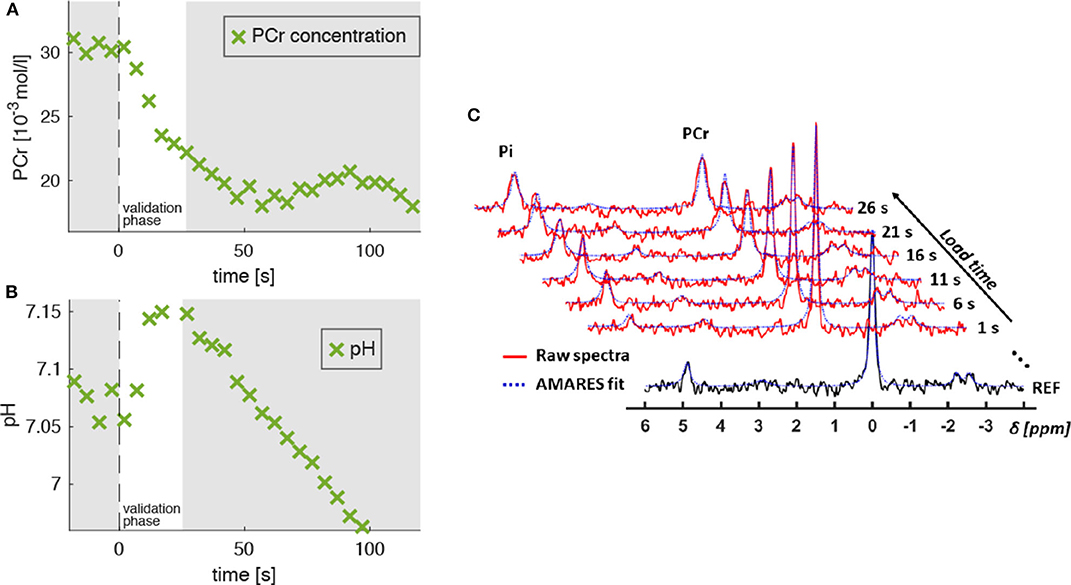
Figure 4. Evolution of PCr concentration ([PCr], A) and pH level (B) extracted from ³¹P-MR spectra, which were acquired in the M. gastrocnemius medialis during dynamic plantarflexion exercise (experiment 3, section 2.3). The time point t = 0 s marks the onset of the exercise. Highlighted is the validation phase (t = 0…25 s) for which we hypothesized agreement between experiment and model. During this phase, the PCr concentration reveals a continuous decrease indicating ATP re-synthesis and, thus, energy consumption in the muscle (see section 2.4). During the validation phase the energy supply is dominated by the PCr depletion. The pH decrease for t > 25 s reflects the H+ accumulation during the anaerobic glycolysis. Subplot (C) shows the raw spectra (red graphs) and corresponding AMARES fits (blue dashed graphs), obtained during the validation phase. The black graph in the sublot (C) shows a spectrum obtained prior to exercise.

Assuming equivalent rates of PCr consumption and ATP synthesis during the validation phase (t < 25s) of the exercise, the amount of energy provided via the ATP hydrolysis can be calculated according to Equation (6). This reveals a steep accumulation of energy with a rate of ${Ė}_{\mathrm{\text{exp}}}=5.8\pm 1.8Jk{g}^{-1}{s}^{-1}$ (Figure 5, linear fit to the experimental data points with t < 25 s, confidence interval 95%). During the later exercise phase, the energy supply is dominated by anaerobic glycolysis and thus cannot be estimated from PCr evolution.

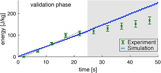
Figure 5. Prediction of the energy consumption by the model (mean: blue line, standard deviation: very small light-blue shade around the blue line) compared to the measured energy consumption in the experiments (derived from the PCr decay; green data points) for dynamic plantarflexion. The model predicts the energy rate (${Ė}_{\mathrm{\text{sim}}}=5.081\pm 0.064Jk{g}^{-1}{s}^{-1}$, linear fit, dotted blue line) as the sum of activation-maintenance heat, shortening-lengthening heat, and mechanical work performed by the muscle fibers: Ė = ḣ_AM + ḣ_SL + ẇ_CE. The experimental data shows a similar energy rate (${Ė}_{\mathrm{\text{exp}}}=5.8\pm 1.8Jk{g}^{-1}{s}^{-1}$, linear fit, dotted green line) during the first 25s (validation phase). During this time, the PCr decay dominates the ATP re-synthesis. Afterwards, the aerobic and anaerobic metabolism additionally contributes (see the progressing pH depletion in Figure 4B). Hence, after 25s not the whole energy consumption is reflected by the measured [PCr] reduction. The error margin for the simulation (light blue) was determined by a Monte-Carlo simulation based on the estimated errors of the subject specific parameters determined in Experiment 1. The error for the experimental energy consumption estimates the maximum error of the ³¹P-MRS.

The energy expenditure rate predicted by the muscle model amounted to ${Ė}_{\mathrm{\text{sim}}}=5.081\pm 0.064Jk{g}^{-1}{s}^{-1}$ (see the blue graph in Figure 4, linear fit). This is in good agreement to the experimental data for the validation phase of the exercise (t < 25 s). The mismatch after the validation phase was expected, as here PCr consumption and ATP synthesis do not have equivalent rates as energy supply is expected to be dominated by anaerobic glycolysisdue. This is indicated by a progressing deviation between simulation and experiment, as they were obtained from the model and PCr time courses, respectively.

Please note, that the time resolution of the simulation is much higher than the time resolution of the experimental data and therefore predicts the small subtle variations in energy rate within every plantarflexion cycle, which is not accessible by the experiment. The estimated model prediction error, as determined by parameter variation, is $\frac{\Delta E}{E}<0.013$ (not even visible in Figure 5 during the validation phase).

5. Discussion

We presented a model that predicts the muscular energy expenditure during dynamic exercise of the human calf muscle and validated this model with metabolic adaptations obtained from in vivo ³¹P-MRS experiments. Generic parameters were taken from literature and subject specific parameters—which reflect the anatomy of the examined subject—were extracted from MRI scans, leaving no free parameter which would require fitting. In order to reproduce the exercise conditions in model based simulations, the model input variables, i.e., the muscle-tendon-unit kinematics and the neuronal muscle stimulation, were defined based on the real experimental data, i.e., on the pedal angulation and EMG recordings. For model validation, we used the spectroscopically extracted rate of PCr depletion, which reflects the ATP synthesis rate in the validation phase of the exercise and, thus, the energy consumption in the muscle.

The main question of the present study whether the applied model can properly reflect the energy expenditure in the loaded muscle can be positively answered in light of the matching between the predicted and experimentally determined energy supply in the validation phase of the exercise.

The increasing mismatch between model prediction and experimental data for t > 25 s was expected, as the PCr break down reflects ATP hydrolysis only during the validation phase of the exercise (Heerschap et al., 1999). The PCr depletion is associated with proton consumption, i.e., the cytosolic pH increase. This situation starts to change in the later phase, where the ATP synthesis is dominated by the anaerobic glycolysis and oxidative phosphorylation. While the latter pathway cannot be directly assessed by means of ³¹P-MR spectroscopy, the onset of the former process is reflected in a steep pH decrease starting approximately 25 s after the exercise begin (see Figure 4B). Our observations are in line with a previous study of Rossiter et al. (2002), who also reported a pH increase from 7.06 to 7.11 after 30 s of exercise onset (see also review by Kemp, 2015). Therefore, the turning point of the pH evolution can be used to set the limits for the time period, during which the predicted and experimentally determined energy supply can be compared. However, as indicated by the constant β-ATP intensities in the ³¹P-MR spectra series, the net cytosolic ATP concentration remained constant throughout the entire exercise period. Thus, we conclude a steady state of ATP hydrolysis and ATP production during the entire time course of the experiment. Furthermore, we assume, as long as the cytosolic pH increases that the ATP production results almost solely from the break-down of PCr.

However, this time window of t < 25 s likely depends on the exercise intensity. At higher intensities (e.g., >20% of single repetition maximum), the PCr breakdown rate will increase and the glycolytic pathways start earlier (<10 s at >90% of single repetition maximum, Barclay 2015).

The advantage of our approach is the possibility to validate the model prediction at the level of individual muscles. Previously, energy expenditure could either be measured in vivo on the organism level (Waters and Mulroy, 1999; Bassett and Howley, 2000; Levine, 2005; Corbett et al., 2008; Au et al., 2009) or estimated from temperature changes for muscle groups (Edwards et al., 1975; González-Alonso et al., 2000; Reitman, 2018). Attempts have been made to combine these measures with musculoskeletal models to estimate how the total energy consumption is distributed between muscles (Umberger, 2010; Miller et al., 2012; Miller, 2014; Dorn et al., 2015; Koelewijn et al., 2019). However, for this purpose it was necessary to estimate and consider the energy consumption outside of muscles as well as the load sharing between muscles. Measuring energy consumption in individual muscles was only possible in in vitro experiments by using isolated animal muscles (Homsher et al., 1975; Curtin and Woledge, 1979). Only one other method has been proposed to measure individual muscular energy consumption in animals in vivo (Marsh, 2006). This method estimates energy consumption from marker particles injected into the blood which accumulate in muscular tissue over time—with the limitation that the measurement can only be performed by dissecting the animal and, thus, allows to estimate an accumulative effect only for the active movement phase shortly before life termination.

5.1. Limitations

5.1.1. Experimental Limitations

Due to the strong magnetic field of the MR scanner, EMG measurements had to be performed in separate trials outside of the scanner. Hence, only very standardized repetitive movements can be investigated and used to validate the model. In addition, the relatively low temporal resolution of ³¹P-MRS series (5 s) prevents the validation of the fine-grained temporal prediction of the muscle model, which resolves the energetic difference between flexion and extension in each cycle (Figure 5). Furthermore, applying the ³¹P-MRS method to a specific muscle requires careful consideration of partial volume effects from other muscles. In this study, the relatively large thickness of the excited spectroscopic slice as well as the leg movements might provoke contaminations of metabolic adaptations in the M. gastrocnemius medialis by contributions from the adjacent muscles M. gastrocnemius lateralis or M. soleus. However, these effects appear to be marginal as the spectroscopic slice captures almost exclusively the M. gastrocnemius medialis (Figure 3). In our study, we used a ³¹P-MRS sequence equipped with a localization scheme, which follows the DRESS technique (Depth-REsolved Surface coil MRS) of Valkovič et al. (2014). A more accurate localization of muscle of interest can be achieved by using a localized semi-LASER dynamic ³¹P-MRS method with selection of well-defined spectroscopic volumes (Fiedler et al., 2015; Niess et al., 2018). However, we decided against the latter approach, since it relies on a spin echo based localization scheme and thus is more susceptible to signal attenuations due to accelerated transverse relaxation of phosphorous metabolites (Meyerspeer et al., 2003).

5.1.2. Robustness Concerning Experimental and Physiological Variations

The model validation is based on the experimental data set of a single subject and one sub-maximal stimulation level only. The model reproduces the experimental data very well. However, subjects with other muscle fiber compositions, training states, etc. could show a different energy expenditure [up to ca. 10% standard deviation for level walking between subjects (Koelewijn et al., 2019)]. Hence, the robustness of our findings concerning inter-individual differences in physiology and anatomy, and for different stimulation levels has to be evaluated in future studies.

5.1.3. Force-Level Validation

The study is currently missing simultaneous validation of the force produced by the muscle. This would require either a direct measurement of the M. gastrocnemius force—which is ethically and technically difficult—or a complete modeling, ³¹P-MR spectroscopic and EMG assessment of all lower leg muscles and subsequent comparison of simulation results with the force time course, which can be measured in the pedal ergometer. For this, also a validation of the muscle's maximum force, e.g., via a dynamometer would be required (Menegaldo and Oliveira, 2012). Therefore, we currently have to rely on the literature, where the muscle model has been validated with respect to force generation in experiments with isolated animal muscles (Günther et al., 2007; Mörl et al., 2012).

5.1.4. Activation Dynamics

Furthermore, the model currently includes activation dynamics, which do not consider fiber-length dependencies. There was a controversy over which activation dynamics are physiologically more relevant. The length-dependent Hatze activation dynamics is strongly supported by experiments on isolated muscles (Rockenfeller et al., 2015). However, if EMG data is used as input to the muscle model, the simpler Zajac activation dynamics may be more appropriate (Kramer, 2012; Menegaldo and Oliveira, 2012). We used the latter in analogy to the original publication of the energy model (Umberger et al., 2003).

5.1.5. Model Parameters

With respect to the model parameters, we confirmed that a variation of the experimentally determined muscle parameters—according to their respective error—has a small effect on the model's energy prediction ($\frac{\Delta E}{E}<0.013$, Figure 5, light-blue shaded area around the simulation results). The normalization of the EMG signal may further influence the predicted energy. Here, we used the maximum voluntary contraction, a standard method for normalization (Menegaldo and Oliveira, 2012). The parameters used to link enthalpy rate with ATP hydrolysis were taken from in vitro experiments under defined conditions (Kodama, 1985) which may differ in in vivo contractions. Moreover, maintenance and shortening heat rates and the fiber type composition largely influence energy output rate. Such parameters are based only on a very small number of studies, and they are variable because different muscle preparations, contraction protocols and methods of measuring were used. Bolstad and Ersland (1978) investigated the rate of temperature rise during voluntary isometric contractions in human M. soleus, M. sarcospinalis, and M. biceps brachii. They found that the heat rate of fast twitch fibers is approximately six times that of slow twitch fibers. Moreover, heat rates depend on temperature (Barclay, 2015) which varies greatly between studies. Even for similar muscle preparations (e.g., mouse M. soleus) at given temperature (20°) the rate of ATP turnover varies by about 80% in different studies (Crow and Kushmerick, 1982; Barclay et al., 2010). Furthermore, muscle activation impacts muscle efficiency and activation costs (Lewis and Barclay, 2014; Barclay, 2015). This variability makes it difficult to select consistent model parameters. In general, used parameters from Umberger et al. (2003) resulted in good prediction of the energy consumption for the performed repetitive submaximal exercise. However, whether this approach (including the chosen parameters) is also applicable for other submaximal contraction levels, other muscles, and other subjects has to be confirmed in future studies.

5.2. Conclusion

In conclusion, the core novelty of our approach is that it allows to validate a model of muscular energy expenditure on a muscle specific level in vivo. We would like to emphasize that this study shows the potential of this approach, but requires intensive future work to validate the model and the approach across subjects, across different muscles, and across different force levels. If valid across all of these factors, the approach offers new possibilities: The muscle model can predict muscular forces and energy expenditure during defined movement regimes. It is even possible to generate forward-dynamic predictions of movements in musculoskeletal simulations which have not been recorded yet. Combining these methods will allow to investigate energy consumption in dynamic movements in much more realistic detail than before (Umberger and Rubenson, 2011). In the future, muscular energy expenditure models may be combined with the energy consumption of the cardio-vascular system to obtain a better model for whole body energetics (Hochstein et al., 2016).

Data Availability Statement

The dynamic datasets generated for this study and the model, including all necessary parameters, are included in the article and the Supplementary Material. The original MRS and MRI data will be provided upon request to the authors.

Ethics Statement

The studies involving human participants were reviewed and approved by Ethics committee of the University Hospital of Jena, Germany. The patients/participants provided their written informed consent to participate in this study.

Author Contributions

DH, SH, AG, SS, TS, and NS: conceptualization. DH, JS, SH, AG, RR, JR, and NS: methodology. DH, JS, and SS: software. JS, SH, AG, TS, RR, JR, and NS: validation. DH, JS, SH, RR, and NS: formal analysis. DH, JS, SH, AG, and NS: investigation. AG, SS, TS, JR, and NS: resources. DH, JS, SH, and NS: data curation. DH, JS, SH, and NS: writing—original draft. DH, JS, SH, AG, SS, TS, RR, JR, and NS: writing—review and editing. DH, JS, SH, AG, and NS: visualization. DH, SH, and NS: supervision. AG and NS: funding acquisition.

Funding

DH was supported by the Ministry of Science, Research, and the Arts Baden-Württemberg (Az: 33-7533.-30-20/7/2). SS was supported by DFG EXC 310. JS and SH were supported by the “Research Seed Capital” of the Ministry of Science, Research and Arts Baden-Württemberg as well as the University of Stuttgart to NS (Az: 33-7533.-30-10/37/1). SS was supported by “Deutsche Forschungsgemeinschaft” (DFG, German Research Foundation) under Germanys' Excellence Strategy - EXC 2075 - 390740016. AG acknowledges funding from the German Research Foundation (DFG, GU 1108/3-1).

Conflict of Interest

The authors declare that the research was conducted in the absence of any commercial or financial relationships that could be construed as a potential conflict of interest.

Acknowledgments

We thank Brian Umberger for sending us the code of his muscle model for comparison. AG, JR, and RR acknowledge support from the Competence Centre for Interdisciplinary Prevention (KIP) at the Friedrich Schiller University Jena and the German Professional Association for Statutory Accident Insurance and Prevention in the Foodstuffs Industry and the Catering Trade (BGN). We acknowledge support by Deutsche Forschungsgemeinschaft and Open Access Publishing Fund of University of Tübingen.

Supplementary Material

The Supplementary Material for this article can be found online at: https://www.frontiersin.org/articles/10.3389/fbioe.2020.00622/full#supplementary-material

References

Arampatzis, A., Karamanidis, K., Stafilidis, S., Morey-Klapsing, G., DeMonte, G., and Brüggemann, G. P. (2006). Effect of different ankle- and knee-joint positions on gastrocnemius medialis fascicle length and EMG activity during isometric plantar flexion. J. Biomech. 39, 1891–1902. doi: 10.1016/j.jbiomech.2005.05.010
Au, S. K., Weber, J., and Herr, H. (2009). Powered ankle - foot prosthesis improves walking metabolic economy. IEEE Trans. Robot. 25, 51–66. doi: 10.1109/TRO.2008.2008747
Barbero, M., Merletti, R., and Rainoldi, A. (2012). Atlas of Muscle Innervation Zones: Understanding Surface Electromyography and Its Applications. Milano: Springer. doi: 10.1007/978-88-470-2463-2
Barclay, C., and Weber, C. (2004). Slow skeletal muscles of the mouse have greater initial efficiency than fast muscles but the same net efficiency. J. Physiol. 559, 519–533. doi: 10.1113/jphysiol.2004.069096
Barclay, C. J. (2015). “Energetics of contraction,” in Comprehensive Physiology (Hoboken, NJ: John Wiley & Sons, Inc.), 961–995. doi: 10.1002/cphy.c140038
Barclay, C. J., Woledge, R. C., and Curtin, N. A. (2010). Is the efficiency of mammalian (mouse) skeletal muscle temperature dependent? J. Physiol. 588, 3819–3831. doi: 10.1113/jphysiol.2010.192799
Bassett, D., and Howley, E. (2000). Limiting factors for maximum oxygen uptake and determinants of endurance performance. Med. Sci. Sports Exerc. 32, 70–84. doi: 10.1097/00005768-200001000-00012
Bhargava, L. J., Pandy, M. G., and Anderson, F. C. (2004). A phenomenological model for estimating metabolic energy consumption in muscle contraction. J. Biomech. 37, 81–88. doi: 10.1016/S0021-9290(03)00239-2
Bolstad, G., and Ersland, A. (1978). Energy metabolism in different human skeletal muscles during voluntary isometric contractions. Eur. J. Appl. Physiol. Occup. Physiol. 38, 171–179. doi: 10.1007/BF00430075
Collins, S. H., Bruce Wiggin, M., and Sawicki, G. S. (2015). Reducing the energy cost of human walking using an unpowered exoskeleton. Nature 522, 212–215. doi: 10.1038/nature14288
Corbett, K., Wilson, J., Aitchison, T., Amjad, A. M., and Grant, S. (2008). A comparison of methods of predicting maximum oxygen uptake. Brit. J. Sports Med. 29, 147–152. doi: 10.1136/bjsm.29.3.147
Crow, M. T., and Kushmerick, M. J. (1982). Chemical energetics of slow- and fast-twitch muscles of the mouse. J. Gen. Physiol. 79, 147–166. doi: 10.1085/jgp.79.1.147
Curtin, N. A., and Woledge, R. C. (1979). Chemical change and energy production during contraction of frog muscle: how are their time courses related? J. Physiol. 288, 353–366.
Dorn, T. W., Wang, J. M., Hicks, J. L., and Delp, S. L. (2015). Predictive simulation generates human adaptations during loaded and inclined walking. PLoS ONE 10:e0121407. doi: 10.1371/journal.pone.0121407
Edwards, R. H., Hill, D. K., and Jones, D. A. (1975). Heat production and chemical changes during isometric contractions of the human quadriceps muscle. J. Physiol. 251, 303–315. doi: 10.1113/jphysiol.1975.sp011094
Ferenczi, M. A., He, Z. H., Chillingworth, R. K., Brune, M., Corrie, J. E., Trentham, D. R., et al. (1995). A new method for the time-resolved measurement of phosphate release in permeabilized muscle fibers. Biophys. J. 68, 191S–192S.
Fiedler, G. B., Meyerspeer, M., Schmid, A. I., Goluch, S., Schewzow, K., Laistler, E., et al. (2015). Localized semi-laser dynamic 31p magnetic resonance spectroscopy of the soleus during and following exercise at 7 t. Magn. Reson. Mater. Phys. Biol. Med. 28, 493–501. doi: 10.1007/s10334-015-0484-5
González-Alonso, J., Quistorff, B., Krustrup, P., Bangsbo, J., and Saltin, B. (2000). Heat production in human skeletal muscle at the onset of intense dynamic exercise. J. Physiol. 524, 603–615. doi: 10.1111/j.1469-7793.2000.00603.x
Günther, M., Schmitt, S., and Wank, V. (2007). High-frequency oscillations as a consequence of neglected serial damping in Hill-type muscle models. Biol. Cybernet. 97, 63–79. doi: 10.1007/s00422-007-0160-6
Haeufle, D. F. B. (2020). Repository of the Open-Source Muscle Model. Available online at: https://github.com/daniel-haeufle/macroscopic-muscle-model
Haeufle, D. F. B., Günther, M., Bayer, A., and Schmitt, S. (2014). Hill-type muscle model with serial damping and eccentric force-velocity relation. J. Biomech. 47, 1531–1536. doi: 10.1016/j.jbiomech.2014.02.009
Hatze, H. (1978). A general myocybernetic control model of skeletal muscle. Biol. Cybernet. 28, 143–157. doi: 10.1007/BF00337136
He, J., Levine, W., and Loeb, G. (1991). Feedback gains for correcting small perturbations to standing posture. IEEE Trans. Autom. Control 36, 322–332. doi: 10.1109/9.73565
Heerschap, A., Houtman, C., in 't Zandt, H. J., van den Bergh, A. J., and Wieringa, B. (1999). Introduction to in vivo 31p magnetic resonance spectroscopy of (human) skeletal muscle. Proc. Nutr. Soc. 58, 861–870. doi: 10.1017/S0029665199001160
Hermens, H. J., Freriks, B., Disselhorst-Klug, C., and Rau, G. (2000). Development of recommendations for SEMG sensors and sensor placement procedures. J. Electromyogr. Kinesiol. 10, 361–374. doi: 10.1016/S1050-6411(00)00027-4
Hochstein, S., Rauschenberger, P., Weigand, B., Siebert, T., Schmitt, S., Schlicht, W., et al. (2016). Assessment of physical activity of the human body considering the thermodynamic system. Comput. Methods Biomech. Biomed. Eng. 19, 923–933. doi: 10.1080/10255842.2015.1076804
Holzbaur, K. R. S., Murray, W. M., and Delp, S. L. (2005). A model of the upper extremity for simulating musculoskeletal surgery and analyzing neuromuscular control. Ann. Biomed. Eng. 33, 829–840. doi: 10.1007/s10439-005-3320-7
Homsher, E., Rall, J. A., Wallner, A., and Ricchiuti, N. V. (1975). Energy liberation and chemical change in frog skeletal muscle during single isometric tetanic contractions. J. Gen. Physiol. 65, 1–21. doi: 10.1085/jgp.65.1.1
Kemp, G. J. (2015). “Muscle studies by 31 P MRS,” in eMagRes (Chichester: John Wiley & Sons, Ltd.), 525–534. doi: 10.1002/9780470034590.emrstm1442
Kemp, G. J., Meyerspeer, M., and Moser, E. (2007). Absolute quantification of phosphorus metabolite concentrations in human muscle in vivo by 31P MRS: a quantitative review. NMR Biomed. 20, 555–565. doi: 10.1002/nbm.1192
Kodama, T. (1985). Thermodynamic analysis of muscle ATpase mechanisms. Physiol. Rev. 65, 467–551. doi: 10.1152/physrev.1985.65.2.467
Koelewijn, A. D., Heinrich, D., and van den Bogert, A. J. (2019). Metabolic cost calculations of gait using musculoskeletal energy models, a comparison study. PLoS ONE 14:e0222037. doi: 10.1371/journal.pone.0222037
Kramer, S. (2012). Modellierung der Muskelkontraktion der Plantarflexoren unter Berücksichtigung physiologischer Parameter und der Muskelarchitektur (Doctoral thesis). Eberhard Karls Universität Tübingen, Tübingen, Germany.
Levine, J. A. (2005). Measurement of energy expenditure. Public Health Nutr. 8, 1123–1132. doi: 10.1079/PHN2005800
Lewis, D. B., and Barclay, C. J. (2014). Efficiency and cross-bridge work output of skeletal muscle is decreased at low levels of activation. Pflügers Arch. 466, 599–609. doi: 10.1007/s00424-013-1344-7
Lichtwark, G. a., and Wilson, a. M. (2005). A modified Hill muscle model that predicts muscle power output and efficiency during sinusoidal length changes. J. Exp. Biol. 208(Pt 15), 2831–2843. doi: 10.1242/jeb.01709
Marsh, R. L. (2006). Partitioning locomotor energy use among and within muscles muscle blood flow as a measure of muscle oxygen consumption. J. Exp. Biol. 209, 2385–2394. doi: 10.1242/jeb.02287
Méndez, J., Keys, A., Mendez, J., and Keys, A. (1960). Density and composition of mammalian muscle. Metabolism 9, 184–188.
Menegaldo, L. L., and Oliveira, L. F. (2012). The influence of modeling hypothesis and experimental methodologies in the accuracy of muscle force estimation using EMG-driven models. Multibody Syst. Dyn. 28, 21–36. doi: 10.1007/s11044-011-9273-8
Meyerspeer, M., Krššák, M., and Moser, E. (2003). Relaxation times of 31p-metabolites in human calf muscle at 3 t. Magn. Reson. Med. 49, 620–625. doi: 10.1002/mrm.10426
Millard, M., Uchida, T., Seth, A., and Delp, S. L. (2013). Flexing computational muscle: modeling and simulation of musculotendon dynamics. J. Biomech. Eng. 135:021005. doi: 10.1115/1.4023390
Miller, R. H. (2014). A comparison of muscle energy models for simulating human walking in three dimensions. J. Biomech. 47, 1373–1381. doi: 10.1016/j.jbiomech.2014.01.049
Miller, R. H., Umberger, B. R., Hamill, J., and Caldwell, G. E. (2012). Evaluation of the minimum energy hypothesis and other potential optimality criteria for human running. Proc. R. Soc. B Biol. Sci. 279, 1498–1505. doi: 10.1098/rspb.2011.2015
Moll, K., Gussew, A., Nisser, M., Derlien, S., Krämer, M., and Reichenbach, J. R. (2018). Comparison of metabolic adaptations between endurance- and sprint-trained athletes after an exhaustive exercise in two different calf muscles using a multi-slice 31 P-MR spectroscopic sequence. NMR Biomed. 31:e3889. doi: 10.1002/nbm.3889
Mörl, F., Siebert, T., Schmitt, S., Blickhan, R., and Günther, M. (2012). Electro-mechanical delay in hill-type muscle models. J. Mech. Med. Biol. 12:1250085. doi: 10.1142/S0219519412500856
Narici, M. V., Binzoni, T., Hiltbrand, E., Fasel, J., Terrier, F., and Cerretelli, P. (1996). In vivo human gastrocnemius architecture with changing joint angle at rest and during graded isometric contraction. J. Physiol. 496, 287–297. doi: 10.1113/jphysiol.1996.sp021685
Niess, F., Fiedler, G. B., Schmid, A. I., Laistler, E., Frass-Kriegl, R., Wolzt, M., et al. (2018). Dynamic multivoxel-localized 31p mrs during plantar flexion exercise with variable knee angle. NMR in Biomed. 31:e3905. doi: 10.1002/nbm.3905
Reitman, M. L. (2018). Of mice and men-environmental temperature, body temperature, and treatment of obesity. FEBS Lett. 592, 2098–2107. doi: 10.1002/1873-3468.13070
Rockenfeller, R., Günther, M., Schmitt, S., and Götz, T. (2015). Comparative sensitivity analysis of muscle activation dynamics. Comput. Math. Methods Med. 2015:585409. doi: 10.1155/2015/585409
Rode, C., Siebert, T., Herzog, W., and Blickhan, R. (2009). The effects of parallel and series elastic components on the active cat soleus force-length relationship. J. Mech. Med. Biol. 09:105. doi: 10.1142/S0219519409002870
Rossiter, H. B., Ward, S. A., Kowalchuk, J. M., Howe, F. A., Griffiths, J. R., and Whipp, B. J. (2002). Dynamic asymmetry of phosphocreatine concentration and O(2) uptake between the on- and off-transients of moderate- and high-intensity exercise in humans. J. Physiol. 541(Pt 3), 991–1002. doi: 10.1113/jphysiol.2001.012910
Rzanny, R., Stutzig, N., Hiepe, P., Gussew, A., Thorhauer, H.-A., and Reichenbach, J. R. (2016). The reproducibility of different metabolic markers for muscle fiber type distributions investigated by functional 31P-MRS during dynamic exercise. Z. Med. Phys. 26, 323–338. doi: 10.1016/j.zemedi.2016.06.006
Saltin, B., and Gollnick, P. D. (1983). Skeletal muscle adaptability: significance for metabolism and performance. Handbook of Physiology. Skeletal Muscle 10, 555–631.
Siebert, T., Rode, C., Herzog, W., Till, O., and Blickhan, R. (2008). Nonlinearities make a difference: comparison of two common Hill-type models with real muscle. Biol. Cybernet. 98, 133–43. doi: 10.1007/s00422-007-0197-6
Siebert, T., Wagner, H., and Blickhan, R. (2003). Not all oscillations are rubbish: forward simulation of quick-release experiments. J. Mech. Med. Biol. 3, 107–122. doi: 10.1142/S0219519403000648
Stefan, D., Cesare, F. D., Andrasescu, A., Popa, E., Lazariev, A., Vescovo, E., et al. (2009). Quantitation of magnetic resonance spectroscopy signals: the jMRUI software package. Meas. Sci. Technol. 20:104035. doi: 10.1088/0957-0233/20/10/104035
Stutzig, N., Rzanny, R., Moll, K., Gussew, A., Reichenbach, J. R., and Siebert, T. (2017). The pH heterogeneity in human calf muscle during neuromuscular electrical stimulation. Magn. Reson. Med. 77, 2097–2106. doi: 10.1002/mrm.26329
Stutzig, N., and Siebert, T. (2016). Reproducibility of electromyographic and mechanical parameters of the triceps surae during submaximal and maximal plantar flexions. Musc. Nerve 53, 464–470. doi: 10.1002/mus.24767
Takashi, R. (1979). Fluorescence energy transfer between subfragment-1 and actin points in the rigor complex of actosubfragment-1. Biochemistry 18, 5164–5169. doi: 10.1021/bi00590a021
Tschiesche, K., Rothamel, M., Rzanny, R., Gussew, A., Hiepe, P., and Reichenbach, J. R. (2014). MR-compatible pedal ergometer for reproducible exercising of the human calf muscle. Med. Eng. Phys. 36, 933–937. doi: 10.1016/j.medengphy.2014.02.026
Umberger, B. R. (2010). Stance and swing phase costs in human walking. J. R. Soc. Interface 7, 1329–1340. doi: 10.1098/rsif.2010.0084
Umberger, B. R., Gerritsen, K. G. M., and Martin, P. E. (2003). A model of human muscle energy expenditure. Computer Methods Biomech. Biomed. Eng. 6, 99–111. doi: 10.1080/1025584031000091678
Umberger, B. R., and Rubenson, J. (2011). Understanding muscle energetics in locomotion: new modeling and experimental approaches. Exerc. Sport Sci. Rev. 39, 59–67. doi: 10.1097/JES.0b013e31820d7bc5
Valkovič, L., Chmelík, M., Just Kukurová, I., Jakubová, M., Kipfelsberger, M. C., Krumpolec, P., et al. (2014). Depth-resolved surface coil MRS (dress)-localized dynamic 31p-MRS of the exercising human gastrocnemius muscle at 7 t. NMR in Biomed. 27, 1346–1352. doi: 10.1002/nbm.3196
van Soest, A., Bobbert, M., Iijima, T., Shimizu, K., and Asanuma, N. (1993). The contribution of muscle properise in the control of explosive movements. Biol. Cybernet. 69, 195–204. doi: 10.1007/BF00198959
Vanhamme, L., van den Boogaart, A., and Van Huffel, S. (1997). Improved method for accurate and efficient quantification of MRS data with use of prior knowledge. J. Magn. Reson. 129, 35–43. doi: 10.1006/jmre.1997.1244
Waters, R. L., and Mulroy, S. (1999). The energy expenditure of normal and pathologic gait. Gait Post. 9, 207–231. doi: 10.1016/S0966-6362(99)00009-0
Wilkie, D. R. (1968). Heat work and phosphorylcreatine break-down in muscle. J. Physiol. 195, 157–183. doi: 10.1113/jphysiol.1968.sp008453
Winters, J. M. (1990). “Hill-based muscle models: a systems engineering perspective,” in Multiple Muscle Systems: Biomechanics and Movement Organization, eds J. M. Winters and S. L-Y. Woo (Berlin; Heidelberg: Springer-Verlag; GmbH & Co. K), 69–93. doi: 10.1007/978-1-4613-9030-5_5
Woledge, R. C., Curtin, N. A., and Homsher, E. (1985). Energetic aspects of muscle contraction. Monogr. Physiol. Soc. 41, 1–357.
Keywords: magnetic resonance imaging (MRI), magnetic resonance spectroscopy, 31P-MRS, plantar flexion, muscle, biomechanical modeling, energy, validation
Citation: Haeufle DFB, Siegel J, Hochstein S, Gussew A, Schmitt S, Siebert T, Rzanny R, Reichenbach JR and Stutzig N (2020) Energy Expenditure of Dynamic Submaximal Human Plantarflexion Movements: Model Prediction and Validation by in-vivo Magnetic Resonance Spectroscopy. Front. Bioeng. Biotechnol. 8:622. doi: 10.3389/fbioe.2020.00622
Received: 03 February 2020; Accepted: 21 May 2020;
Published: 26 June 2020.
Edited by:
Fabio Galbusera, Istituto Ortopedico Galeazzi (IRCCS), ItalyReviewed by:
Glen Lichtwark, The University of Queensland, AustraliaMohammad Nikkhoo, Islamic Azad University, Iran
Marek Chmelik, University of Prešov, Slovakia
Copyright © 2020 Haeufle, Siegel, Hochstein, Gussew, Schmitt, Siebert, Rzanny, Reichenbach and Stutzig. This is an open-access article distributed under the terms of the Creative Commons Attribution License (CC BY). The use, distribution or reproduction in other forums is permitted, provided the original author(s) and the copyright owner(s) are credited and that the original publication in this journal is cited, in accordance with accepted academic practice. No use, distribution or reproduction is permitted which does not comply with these terms.
*Correspondence: Daniel F. B. Haeufle, daniel.haeufle@uni-tuebingen.de