Prediction of Maximum Flood Inundation Extents With Resilient Backpropagation Neural Network: Case Study of Kulmbach

Lin, Qing; Leandro, Jorge; Wu, Wenrong; Bhola, Punit; Disse, Markus

doi:10.3389/feart.2020.00332

ORIGINAL RESEARCH article

Front. Earth Sci., 05 August 2020
Sec. Hydrosphere
Volume 8 - 2020 | https://doi.org/10.3389/feart.2020.00332

Prediction of Maximum Flood Inundation Extents With Resilient Backpropagation Neural Network: Case Study of Kulmbach

Qing Lin^*

Jorge Leandro

Wenrong Wu

Punit Bhola

Markus Disse

Department of Civil, Geo and Environmental Engineering, Technical University of Munich, Munich, Germany

In many countries, floods are the leading natural disaster in terms of damage and losses per year. Early prediction of such events can help prevent some of those losses. Artificial neural networks (ANN) show a strong ability to deal quickly with large amounts of measured data. In this work, we develop an ANN for outputting flood inundation maps based on multiple discharge inputs with a high grid resolution (4 m × 4 m). After testing different neural network training algorithms and network structures, we found resilience backpropagation to perform best. Furthermore, by introducing clustering for preprocessing discharge curves before training, the quality of the prediction could be improved. Synthetic flood events are used for the training and validation of the ANN. Historical events were additionally used for further validation with real data. The results show that the developed ANN is capable of predicting the maximum flood inundation extents. The mean squared error in more than 98 and 86% of the total area is smaller than 0.2 m² in the prediction of synthetic events and historical events, respectively.

Introduction

Flood is one of the most damaging natural hazards hitting settlements which threatens the safety of civilians and the integrity of infrastructures (Berz, 2001). Flooding is the leading cause of damage and losses in many countries in the world (Kron, 2005). Furthermore, as a result of climate and land-use changes, the flood vulnerability of some regions is expected to rise (Vogel et al., 2011). Accurate prediction of floods in urban areas can contribute to the development of essential tools to minimize the risks of flooding.

There are different types of numerical models widely used for urban flood simulation (Henonin et al., 2013). Hydrological rainfall run-off models can be used to simulate distributed river discharges. One-dimensional (1D) drainage model solving the one-dimensional Saint-Venant flow equations, can be applied for simulating the surcharge or drainage of the underground drainage network (Mark et al., 2004). The two-dimensional (2D) Saint-Venant flow equations are ideal tools for simulating the urban surface inundation, and obtain the maximum flood extents, maximum depths and flow velocity on many points on the surface. Furthermore, the 1D–2D coupling model simulates the drainage network and the urban surface simultaneously. Even though they provide more accurate results than the previous models (Hankin et al., 2008), they are computationally more expensive. All approaches require field measurements for defining the model parameters. The two latter have prohibitive high computation costs and require very detailed data sets which often restrict the application for real-time forecasting (Vogel et al., 2011). With the advances in high-performance computing, graphics processing units (GPU) nowadays are capable of faster 2D simulation in much larger areas (Kalyanapu et al., 2011). Although these scalability techniques reduce the simulation time greatly, it is still unacceptably high in many cases for real-time early warning systems.

Data-driven approaches can be a feasible alternative for established flood simulation models (Mosavi et al., 2018). Unlike conventional numerical models, data-driven models require input/output data only. The fast-growing trend of data-driven models has shown their high performance even for nonlinear problems (Mekanik et al., 2013). Unlike physical-based models, data-driven models do not require field measurements for determining (physically based) model parameters, which alleviates the burden on the users for data gathering and model setup. ANN can be a useful tool for modeling, if properly applied. Indeed some of the pitfalls are the likelihood of over-fitting or under-fitting the data, and insufficient length of the data sets which may lead to erroneous model results (Zhang, 2007). Various data-driven models for short and long term flood forecasts have been developed using neuro-fuzzy (Dineva et al., 2014), support vector machine (SVM) (Bermúdez et al., 2019), support vector regression (Gizaw and Gan, 2016; Taherei et al., 2018) and artificial neural network (ANN) (Kasiviswanathan et al., 2016). Artificial neural network is a popular approach in flood prediction (Elsafi, 2014; Abbot and Marohasy, 2015). Some works have successfully applied ANN for forecasting water levels. Dawson and Wilby (2001) applied ANN to conventional hydrological models in flood-prone catchments in the United Kingdom in 1998. Since then, many studies about flood forecasts in catchment scales arose (Chang L.C. et al., 2018; Yu et al., 2006). Thirumalaiah (1998) compared the water level forecast results along a river using backpropagation, conjugate gradient as well as cascade correlation. Coulibaly et al. (2000) combined Levenberg-Marquardt Backpropagation (Marquardt, 1963) with cross-validation to prevent the under-fitting and overfitting in daily reservoir inflow forecasting. Taghi et al. (2012) applied a backpropagation network and a time lag recurrent network having reached a similar forecast precision in reservoir inflow. Humphrey et al. (2016) joined a conceptual rainfall-runoff model with a Bayesian artificial neural network for improving the precision of the neural network. Sit and Demir (2019) used discretized neural networks for the entire river network in Iowa. By including more location information, they could enhance the forecasting results. Bustami et al. (2007) applied backpropagation ANN model for forecasting water level at gaging stations. Tiwari and Chatterjee (2010) compared different types of ANN predictions of water levels at gaging stations, namely a wavelet-based, a bootstrap based and a hybrid wavelet-bootstrap-ANN (WBANN) and shown that the WBANN model was more accurate and reliable compared to other three ANN. For flood inundation forecast, Simon Berkhahn et al. (2019) trained an ANN with synthetic events of spatial rainfall data for 2D urban pluvial inundation. Chang M.J. et al. (2018) applied a mix of SVM and GIS analysis to expand point forecasts to flooded areas at a sub-catchment scale. Chu et al. (2020) proposed an ANN-based framework for flood inundation prediction based on single inflow data for a 20 m × 20 m grid resolution.

In this article, we develop a method for predicting the maximum flood inundation in an urban area by backpropagation networks based on multiple inflow data for a grid resolution of 4 m × 4 m. Unlike most of the previous studies, this work focuses on applying ANN in an urbanized area for producing high-resolution flood inundation maps from river flooding. For the prediction of maximum flood inundation, only the real-time discharges of the upstream catchments are needed. In Methodology, we introduce the backpropagation artificial neural network, fuzzy c-means clustering methods (FCM) and our criteria for model evaluation. Study Area and Dataset provides basic background information about our study area as well as the synthetic event database for our model training. Results shows the results of our model tuning, the simulation results for synthetic and historical events. To improve the model training behavior by a limited database, we introduce two FCM for the preprocessing of the training dataset. Last sections are the discussion and conclusion of this work.

Methodology

Resilient Backpropagation Algorithm for Artificial Neural Network

The ANN applied in this work for modeling the study area is a forward-feed neural network (FNN) (Nawi et al., 2007), producing and transmitting the data in a network structure. The basic element of the neural network is the neuron. Each neuron collects values from the previous layer by summing up the results from the previous neuron values multiplying the weight on each input arc and storing the results on itself. Through multiple layered neurons, information is proceeded by the weights and transferred over the network, finally reaching the output layer. The input layer of all ANNs is given by seven inflows upstream contributing to the urban area of Kulmbach from the event database (further details can be found in “HEC-RAS and Synthetic Event Database” section). The output layer is set from the raster flood inundation map from the event database.

Backpropagation is an algorithm widely applied in neural network studies, for optimizing the weights in forward-feed neural networks (Nawi et al., 2007). The procession consists of two phases: the training phase collects a part of data from the existing database, tuning the model by changing the weights on input arcs to minimize the bias on the output layer; the recalling phase produces the new outputs for the testing inputs. The rest individuals in the training dataset are used for evaluating the behavior of the network. The total bias between the output of ANN and the observed values is defined as the error function. In order to reduce the error function in each iteration, the weights are modified automatically as described below. The chain rule is applied for minimizing the biases, namely written as:

\frac{\partial L}{\partial w_{ij}} = \frac{\partial L}{\partial O_{i}} \cdot \frac{\partial O_{i}}{\partial {net}_{i}} \cdot \frac{\partial {net}_{i}}{\partial w_{ij}} (1)

where

L is error function of the model.

W_ij is weight from i’th neuron to j’th neuron.

O_i is output of the model.

net_i is weighted sum of the inputs of neuron i.

w_{ij} (t + 1) = w_{ij} (t) - ϵ \cdot \frac{\partial L}{\partial w_{ij}} (t) (2)

where

ϵ is learning rate taken as 0.01 in our training.

The learning rate is used for scaling the gradient in each iteration of the weight update. It is critical to pick up the correct value. A large learning rate will miss the optimal point, while a small learning rate would slow the training process. Herein, we apply the gradient descent algorithm to calculate the update of the weights. To speed up the convergence of the iteration formula (2), resilient backpropagation as defined in Saini (2008) is applied, which treats the update of weights differently depending on the derivative of the error function. Larger alternative learning rate η⁺ could be set for speeding up the iterations if the error gradient remains in the same direction in neighboring time-steps and smaller alternative learning rate η⁻ when approaching the optimal weights.

Δ_{ij} (t) = {\begin{matrix} η^{+} \cdot Δ_{ij} (t - 1), \frac{\partial L}{\partial w_{ij}} (t) \cdot \frac{\partial L}{\partial w_{ij}} (t - 1) > 0 \\ η^{-} \cdot Δ_{ij} (t - 1), \frac{\partial L}{\partial w_{ij}} (t) \cdot \frac{\partial L}{\partial w_{ij}} (t - 1) < 0 \\ Δ_{ij} (t - 1), e l s e \end{matrix} (3)

w_{ij} (t) = {\begin{matrix} w_{ij} (t - 1) + Δ_{ij} (t), \frac{\partial L}{\partial w_{ij}} (t) < 0 \\ w_{ij} (t - 1) - Δ_{ij} (t), \frac{\partial L}{\partial w_{ij}} (t) > 0 \\ 0, e l s e \end{matrix} (4)

In which 0 < η⁻ < 1 < η⁺. In our study these were set constant and equal to $η^{-} = 0.5, η {}^{+}= 1.2$ .

Due to the total number data of pixels (resolution of 4 by 4 m) in the city of Kulmbach, a single hidden layer would exceed 365 thousand elements. To reduce the storage requirement and the ANN model training time, the study area is subdivided into 50 × 50 squared grids, each grid having its own independent ANN (the output layer has 1400 elements) (Figure 1). A similar strategy was used by Berkhahn et al. (2019) for an ANN for flood prediction having rainfall as input.

FIGURE 1

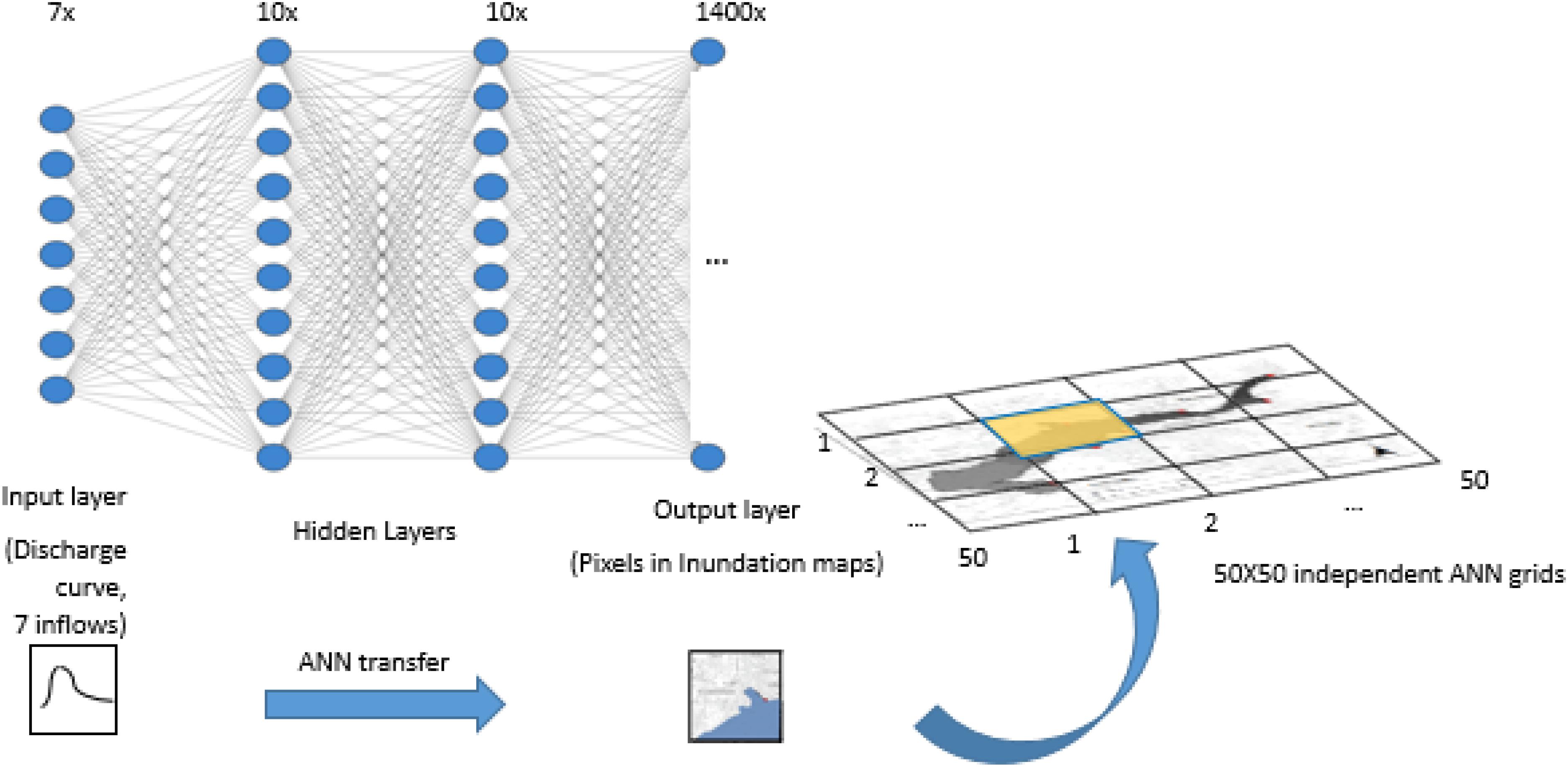
Figure 1. Neural network setups. The study area is divided in 50 × 50 raster each simulated by its own ANN. Input layer: seven input hydrographs. Output layer: flood inundation extent in each grid.

Fuzzy C-Means Clustering and Principal Component Analysis

To further enhance the ANN behavior, we apply clustering to the discharges training dataset. Therefore, we can reduce the size of the training dataset while still keeping the main representative events. As such the training time can be reduced and the overfitting effects minimized. Fuzzy C-means clustering (FCM) (Tilson et al., 1988) is a widely used clustering method, which avoids the deficit of the sub-clusters with unequivocal similarities within its components (Mukerji et al., 2009). In FCM, every single event is given a membership u, which indicates the relation between the event and a certain cluster. If a membership is equal to zero, it means that the event has nothing in common to a specific cluster; if the membership is one, the event is located at the center of the cluster. Once a cluster is set up, the membership u can be calculated by the following equations, and based on the event and the distances between the events. For cluster i and event j, the membership u_ij is to quantify distances between events and cluster centers.

{\begin{matrix} u_{ij} \in [0, 1] \\ \sum_{i = 1}^{c} u_{ij} = 1, 1 < j \leq n \end{matrix} (5)

u_{i j}^{(k)} = \frac{1}{\sum_{r = 1}^{} c {(\frac{d_{i j}^{(k)}}{d_{r j}^{(k)}})}^{2}} (6)

d_{ij} = {|| x_{j} - v_{i} ||}^{2} (7)

v_{i} {}^{(k + 1)}= \frac{\sum_{j = 1}^{n} u_{ij}^{(k)} x_{j}}{\sum_{j = 1}^{n} u_{ij}^{(k)}} (8)

where

c is number of clusters, 2 ≤ c ≤ n − 1.

v_i is centroid of i-th cluster.

d_ij is Euclidean distance between event j and its corresponding centroid.

For optimal clustering, the total sum of distances between events and the cluster centroids have to be the minimum possible. Therefore the following objective function needs to be optimized:

J_{m} (U, V) = \sum_{j = 1}^{n} \sum_{i = 1}^{c} {(u_{ij})}^{2} d_{ij} (9)

Two approaches are applied for deciding the clustering parameters: (a) conventional clustering (by pre-selected hydrograph characteristic parameters); (b) dimension reduction methods. In the former, the clustering variables chosen were P (peak discharge value), T (peak time), V (total volume), V24 (volume in the first 24 h). These can be applied individually or combined. The latter clustering method is based on principal component analysis among the hydrographs. The data are projected to the first several principal eigenvectors for dimensionality reduction via PCA, for further clustering by FCM. To determine the optimal number of clustering c, we define the clustering performance index L(c).

L (c) = \frac{\sum_{i = 1}^{c} (\sum_{j = 1}^{n} u_{ij}^{2}) {|| v_{i} - \bar{x} ||}^{2}}{\sum_{i = 1}^{c} \sum_{j = 1}^{n} u_{ij}^{2} {|| v_{i} - x_{j} ||}^{2}} \cdot \frac{n - c}{c - 1} (10)

The optimal cluster number c can be determined by the maximum of L(c).

Model Evaluation

To evaluate the performance of the ANN prediction of maximum flood inundation in the study area is based on the mean squared error (MSE) of each grid. It is assumed that the inundation maps from the synthetic events produced using a dynamic model (HEC-RAS) are the observed values. The synthetic events have been produced using the FloodEvac-Tool (Bhola et al., 2018). The model has been validated (Bhola et al., 2019). As each grid has its own independent training network, the MSE is evaluated using all the pixels in each grid.

MSE = \frac{1}{n} \sum_{i = 1}^{n} {(T - S)}^{2} (11)

where

T is predicted value.

S is observed value.

To evaluate the overall behavior of the model across the training and validation data sets, the average of MSE and the standard deviation of MSE are evaluated, indicating the average accuracy and the spread of the ANN predictions.

avg . {MSE}^{m} = \frac{1}{N} \sum_{n = 1}^{N} {MSE}_{n}^{m} (12)

where

m is grid index.

n is pixel index in a grid.

N is total number of pixels.

Study Area and Dataset

Study Area

The study area of Kulmbach is located by the river Main in Bavaria. The city consists of northern and southern parts split by the White Main crossing it. About 27 thousand inhabitants live in this city. The city is classified as a great district city with a population density of 292 inhabitants per km² in the area of 92.77 km². On May 28, 2006, Kulmbach was heavily flooded from the river and streams nearby. This event was the trigger for decision-makers to review the initiatives of flood prevention for the city. There are seven streams contributing to this area, namely the Red Main, Schorgast, Dobrach, White Main, Kinzelsbach, Kohlenbach, and Mühlbach. The inflows of the seven streams used for training the ANN are the same ones used in the boundary conditions of the hydraulic model. Hence, the two approaches are comparable. The training-validation of the 50 × 50 ANN aims to replace the hydraulic processes within the marked study area (see Figure 2). Each ANN aims to generate the inundation map for one sub-divided area. All the inflows are inputted to all the networks to keep the ANN topology identical, and thus avoiding the sudden jump of forecasted water depths at ANN borders (Chu et al., 2020). Since the ANNs are trained on the same data, and using the same inflows as inputs, the inundation maps across the different ANNs are consistent.

FIGURE 2

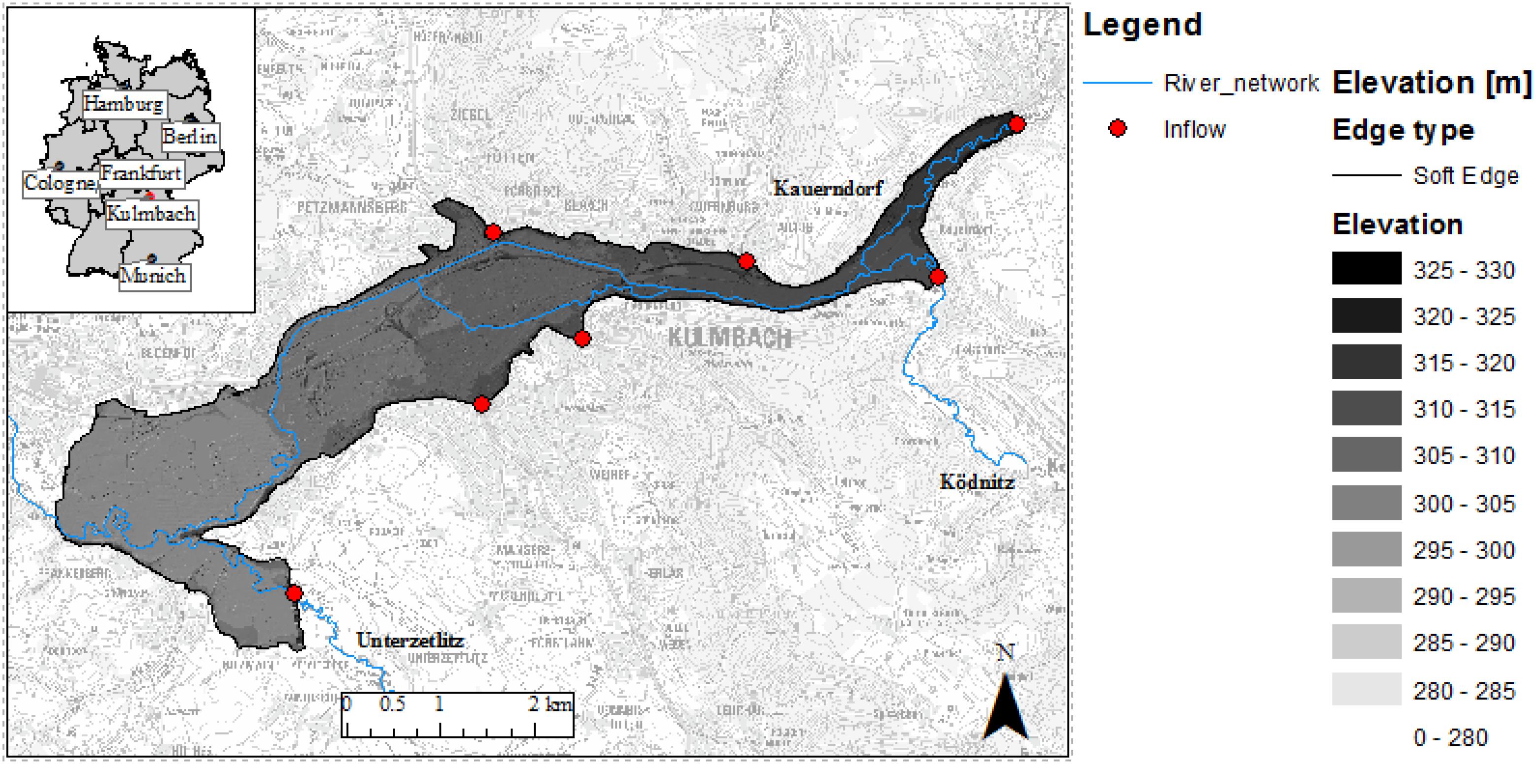
Figure 2. Map of the study area. It shows the location of Kulmbach in Germany. The blue curves represent the river network. The shaded region is the study area with its topography represented. On the marked boundary, the red points represent the seven inflow boundary conditions (three rivers and four smaller streams).

HEC-RAS and Synthetic Event Database

The synthetic event database is generated by the 2D hydraulic model HEC-RAS (Hydrologic Engineering Center – River Analysis System, Davis, CA, United States) for various rainfall intensities, distribution, duration (Bhola et al., 2018). The synthetic events are generated following two stages. First, the hydrologic model LARSIM (Large Area Runoff Simulation Model) (Ludwig and Bremicker, 2006) is used for calculating the discharge hydrographs into the city area. LARSIM is a hydrological model applied for flood forecasting at the Bavarian Environment Agency (Disse et al., 2018). Afterward, the 180 convective and advective events are simulated with the 2D hydraulic model HEC-RAS 2D to generate the flood inundation map database. The maps are generated with high temporal resolution (15 min) and projected to a spatial resolution of 4 by 4 m. For further details of the generation of synthetic events please refer to Bhola et al. (2018).

Results

ANN Training Algorithm

Two training algorithms are applied for training the ANN model using the same training dataset (Event #1–#120): resilient backpropagation (RP) and the conjugate gradient (CGF). After that, both generated models are evaluated using the MSE over the remaining runs (60) in the testing dataset (Event #121–#180) (see Figure 3). Figure 4 shows the MSE evaluated over the training dataset just for comparison purposes. In Figures 3A,B, most grids have the MSE lower than 0.2 m², showing that both RP and CGF networks behave well in general. Figure 4 shows the MSE from RP is mostly better than that of CGF.

FIGURE 3

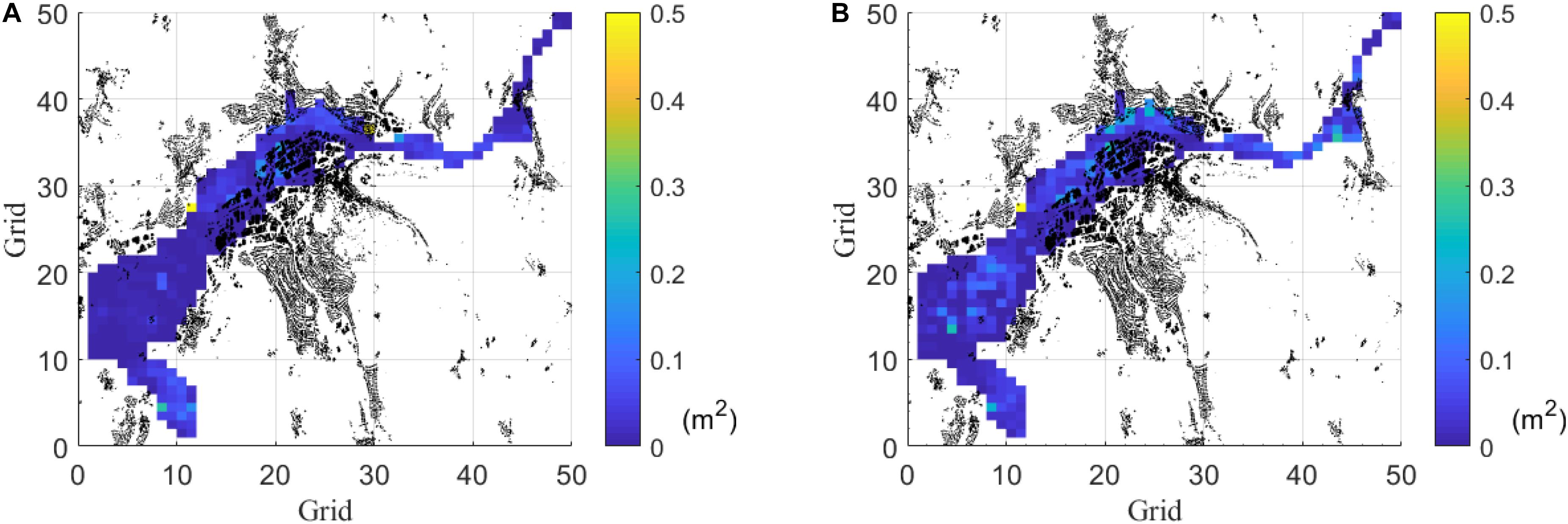
Figure 3. Comparison of average MSE by the two training algorithms in the testing dataset (Event #121 to Event #180). Each grid is an ANN. Black elements are houses. (A) Average (among events) MSE by resilient backpropagation (RP). (B) Average (among events) MSE by conjugate gradient (CGF).

FIGURE 4

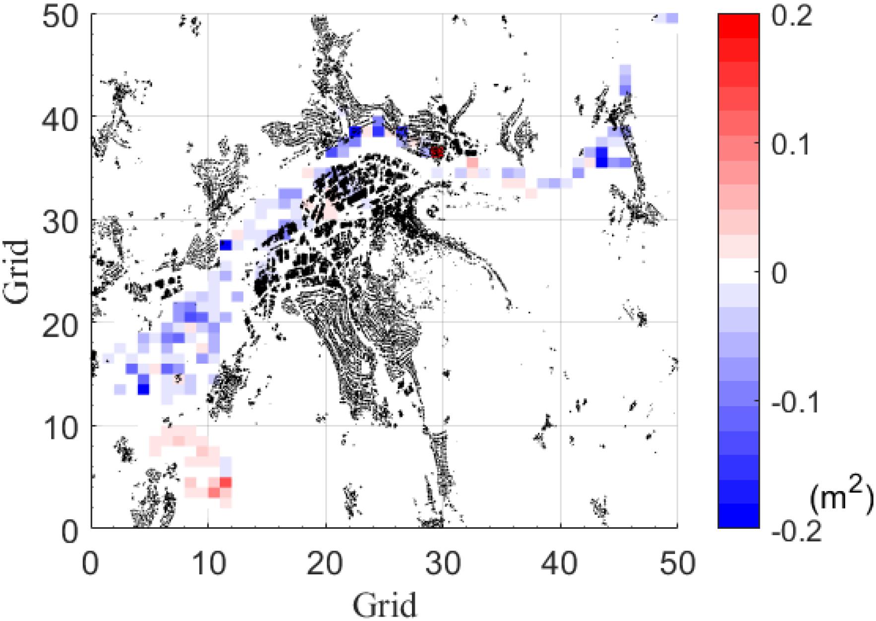
Figure 4. Difference of average MSE by the two training algorithms in the training dataset (Event #1 to Event #120). Each grid is an ANN. Black elements are houses. Negative values indicate that RP performs better than CGF (i.e., smaller MSE). In the plot, 149 grids have positive values and 335 grids have negative values.

Number of Hidden Layers and Neurons

To improve the performance of the neural networks, the layer number and neuron number for comparison are modified. By optimizing the error function with the training dataset, the optimized number of network layers and neurons per layer are obtained. The layer number is set between two to six, while the neuron number set from 10 to 30. Table 1 shows the number of grids in each combination (number layers and neurons) which outperform all the others; it shows 70% of all grids fall within the number of layers equal to two or three layers.

TABLE 1

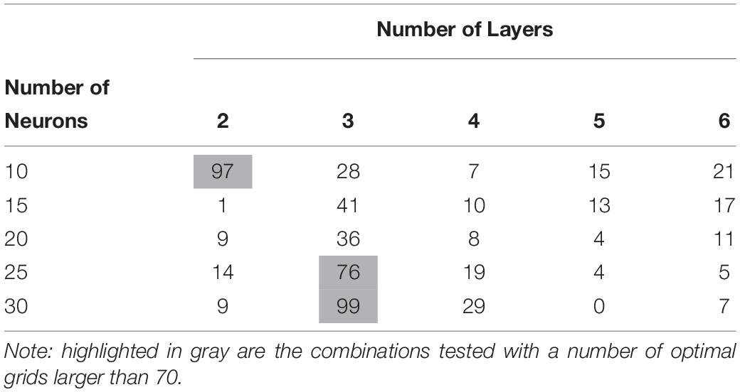
Table 1. Number of grids in each combination (number layers and neurons) which outperform all the others.

Grid Resolution

The grid resolution comparison aims to verify if a finer grid improves the prediction performances. Two grid sizes are tested, namely one with 50 × 50 (each grid has 1400 pixels) and another with 100 × 100 (each grid as 350 pixels) grids (Figure 5). The former has 2500 ANN networks that need to be trained, while the latter has 10000. Since the 50 × 50 performed better (see Table 2) and is computationally more efficient, the former is selected for this study.

FIGURE 5

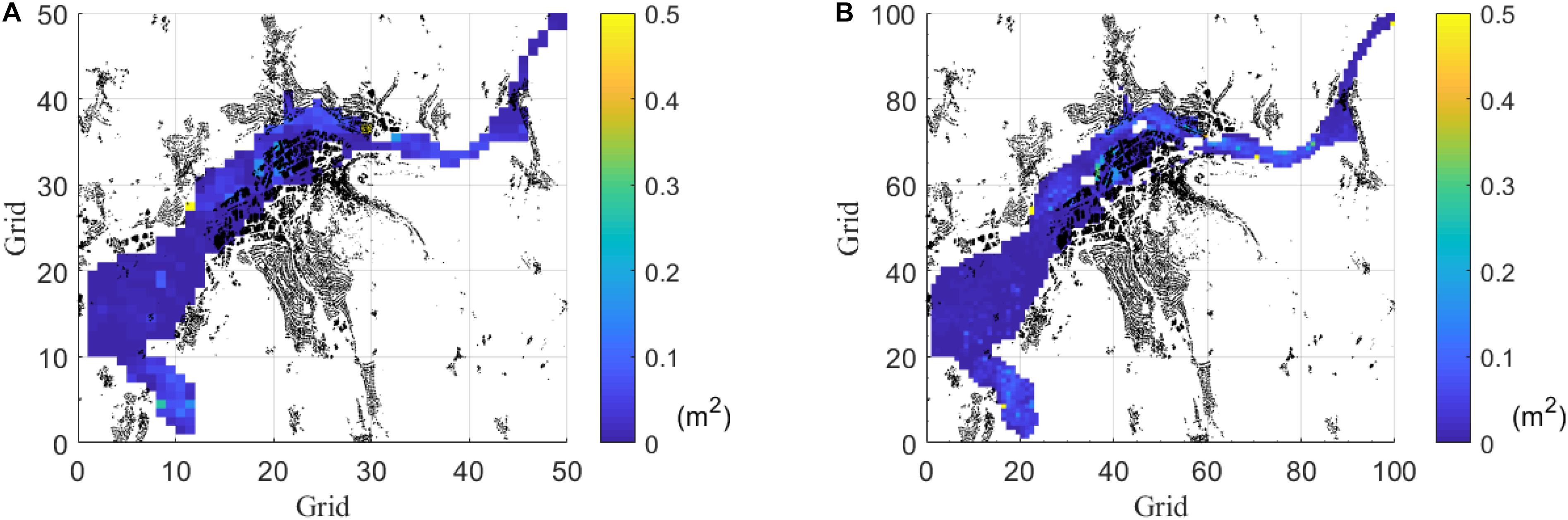
Figure 5. Comparison of average MSE by two grid-size (numbers of ANNs) in the testing dataset (Event 121 to Event #180). Black elements are houses. (A) Average (among events) MSE in 50 × 50 grids by RP. (B) Average (among events) MSE in 100 × 100 grids by RP.

TABLE 2

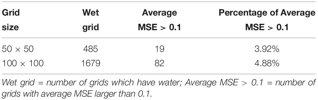
Table 2. The impact of grid size on the ANN training.

Fuzzy C-Means (FCM) Clustering

Here different results from clustering different sets of parameters obtained from the hydrographs are evaluated using the index L(c) (Tilson et al., 1988). Larger numbers indicate that the selected parameters are more suitable. Figure 6A shows the relationship between the index L(c) and the clustering number. The spreads of the 90% confidence intervals of the clusters are listed in Table 3. According to Table 3, the clustering by four parameters (P, V, V24, T) produces the minimum spread, which is the best clustering parameter combination for our studies. Figure 7 also shows that the 90% confidence interval of the four clusters by conventional FCM according to the parameter combination of (P, V, V24, T) is the best choice. Besides the conventional FCM, FCM is also quantified based on principal component analysis (PCA-FCM). It is observed that by choosing seven components for clustering we can represent more than 97% of the original data (Figure 6B). The clustering results by PCA-FCM are shown in Figure 8. The comparison in Table 3 shows that PCA-FCM generates smaller integrals of the bandwidth area (i.e., the 90% confidence interval shown in Figure 8) than those of the conventional FCM. The integral of the bandwidth area is a measure of the spread of the discharge curves in each cluster. An efficient clustering strategy will have a small spread. As such the clusters generated by PCA-FCM are applied in this study. Table 4 summarizes the sign of the differences among the training results from 100 clustered events to those from original unclustered 120 events and a random unclustered 100 events.

FIGURE 6

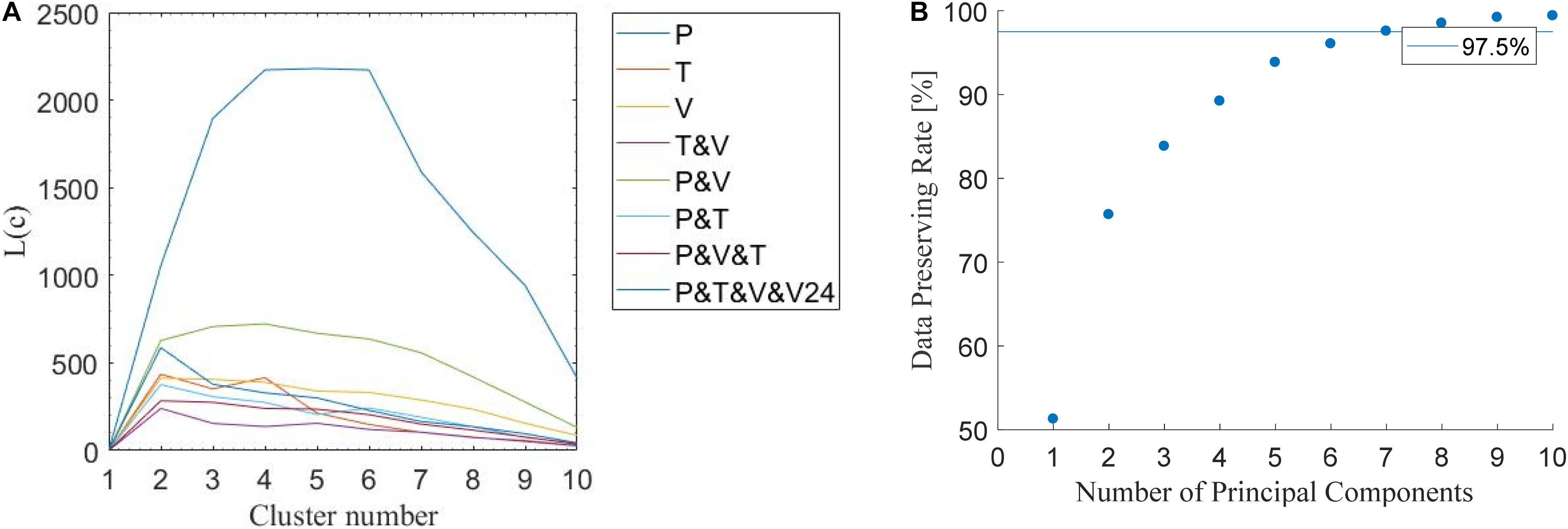
Figure 6. Determine cluster numbers and numbers of principal components. (A) Conventional FCM criteria and their corresponding L(c) values: P (peak discharge value), T (peak time), V (total volume), and V24 (volume in the first 24 h). (B) Data preserving rate in relation to the numbers of principal components. A minimum data-preserving rate of 97.5% was selected as a good representation of the training database.

TABLE 3

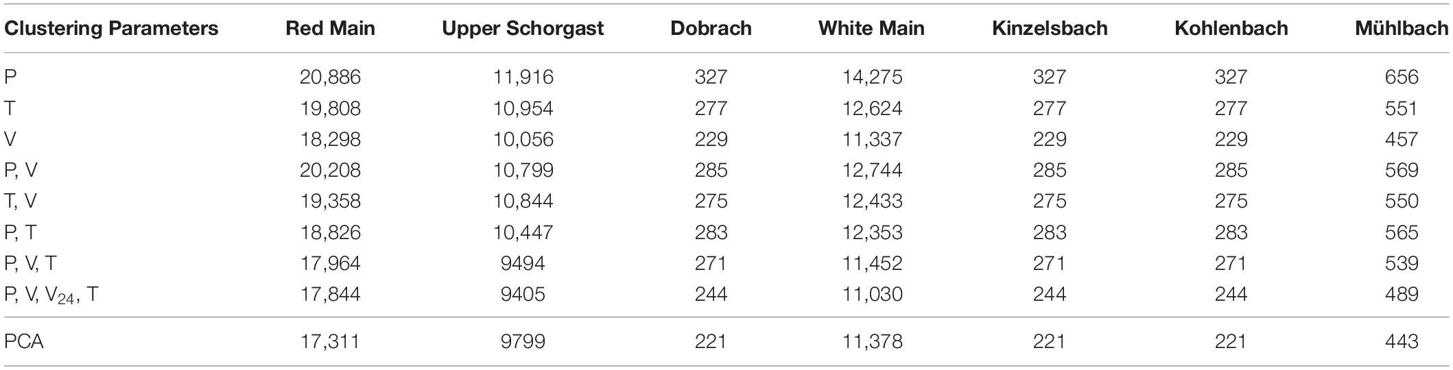
Table 3. Integral of the bandwidth (90% confidence interval shown in Figure 9) by conventional FCM and PCA-FCM assuming a cluster number equal to 4.

FIGURE 7

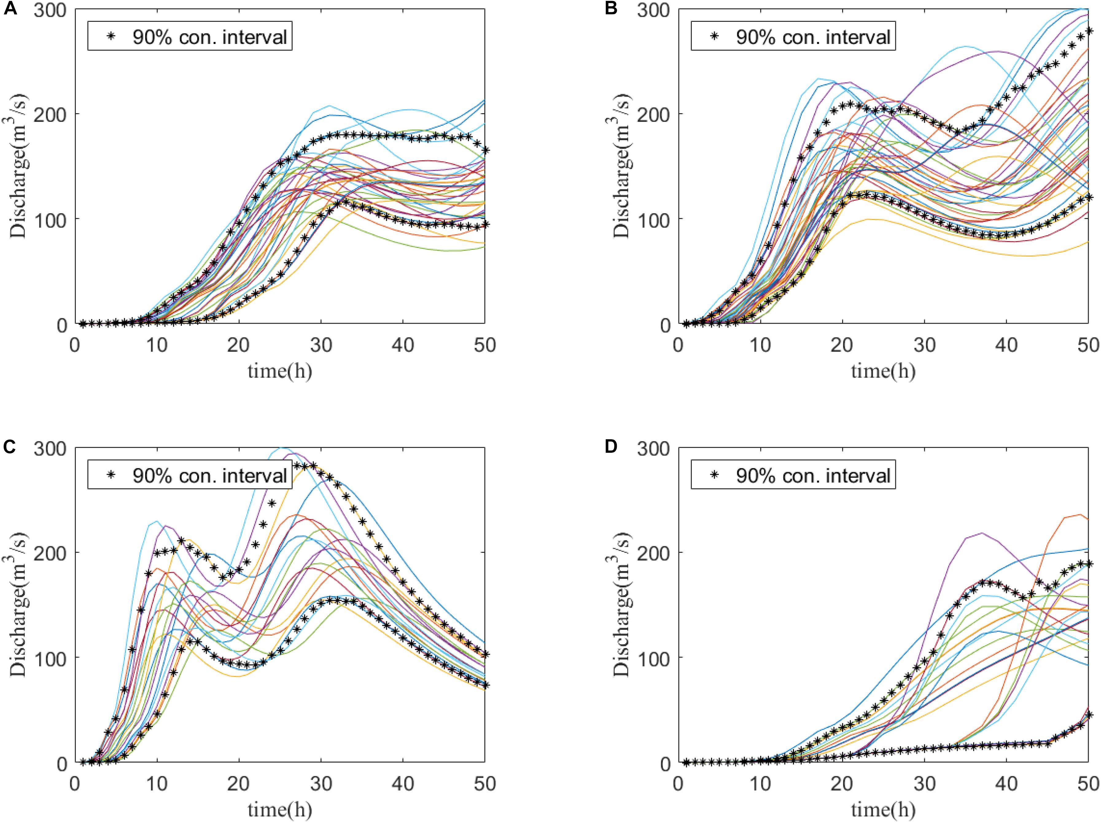
Figure 7. Clustering of all the discharge curves in the training dataset of Stream Red Main (biggest inflow) grouped into four clusters by conventional FCM. Each curve represents a single event. (A–D) The curves are clustered into the above four clusters. The clustering is based on the combination of P (peak discharge value), T (peak time), V (total volume), and V24 (volume in the first 24 h). Asterisks represent the 90% confidence intervals of the four clusters (A–D).

FIGURE 8

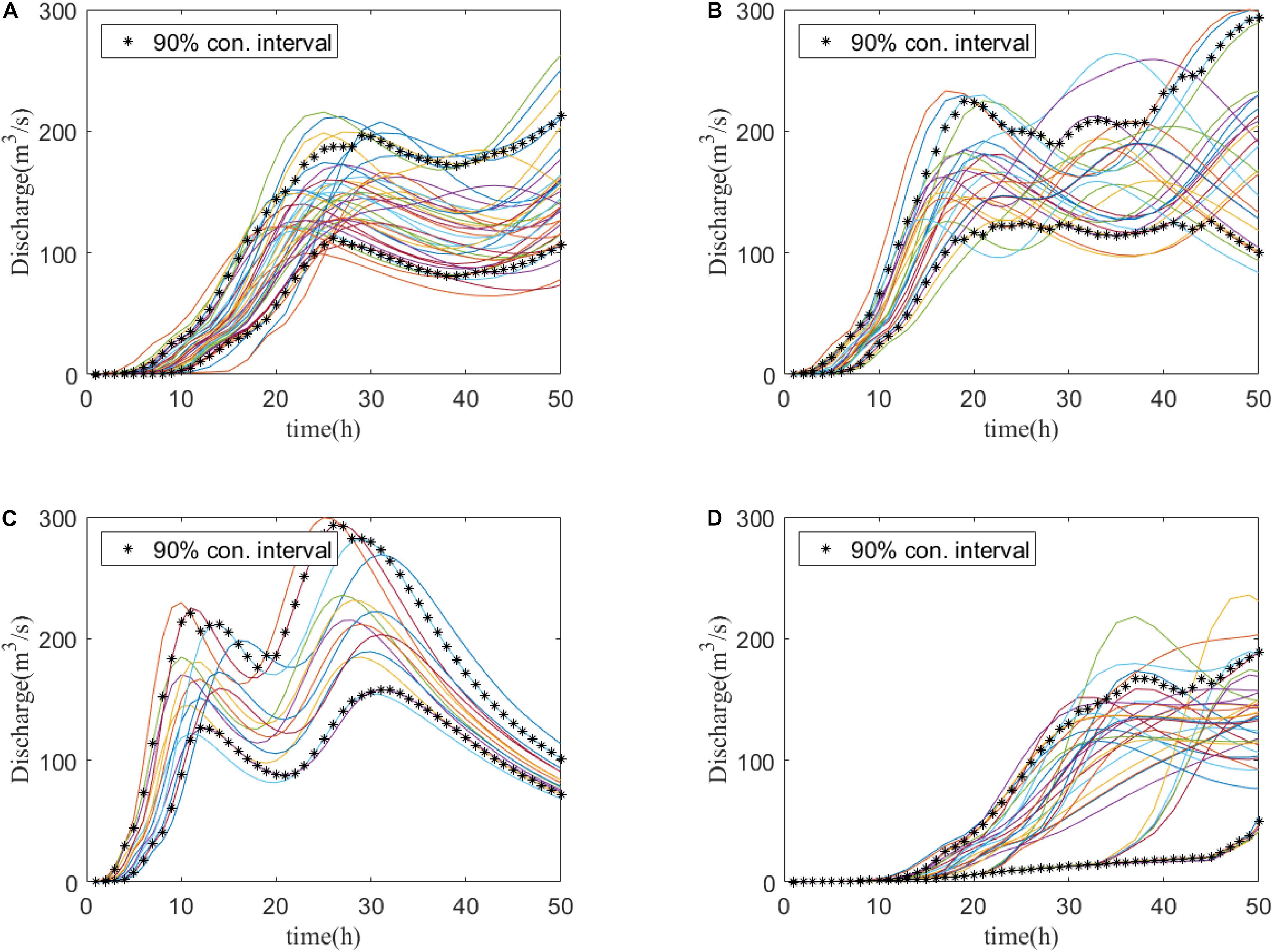
Figure 8. Clustering of all the discharge curves in training dataset of Stream Red Main (biggest inflow) into four clusters by PCA-FCM. Each curve represents a single event. (A–D) The curves are clustered into the above four clusters. Asterisks represent the 90% confidence intervals of the four clusters (A–D).

TABLE 4

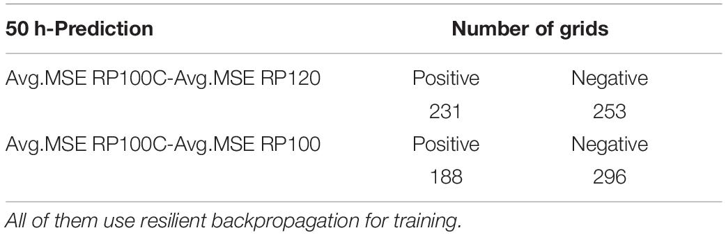
Table 4. Sign of MSE difference between PCA-FCM clustered 100 events, original 120 events, and the randomly clustered 100 events.

Prediction of Maximum Flood Inundation for Synthetic Events

For the sake of representation of results, Figure 9 shows one example of the comparison of the flood inundation maps of one single event, Event 180. It is visually possible to infer that the flood inundation maps and water depths from the ANN and the ones from the HEC-RAS database are very similar. To study the overall performance across all 60 events in the testing set, the average and standard deviation of MSE of every testing event in the whole area is evaluated. In Figure 3A, most of the area is displayed blue, showing that the MSE is close to 0.1 m². Overall, only 1.21% (seven out of 580) of total grids have their MSE over 0.2 m².

FIGURE 9

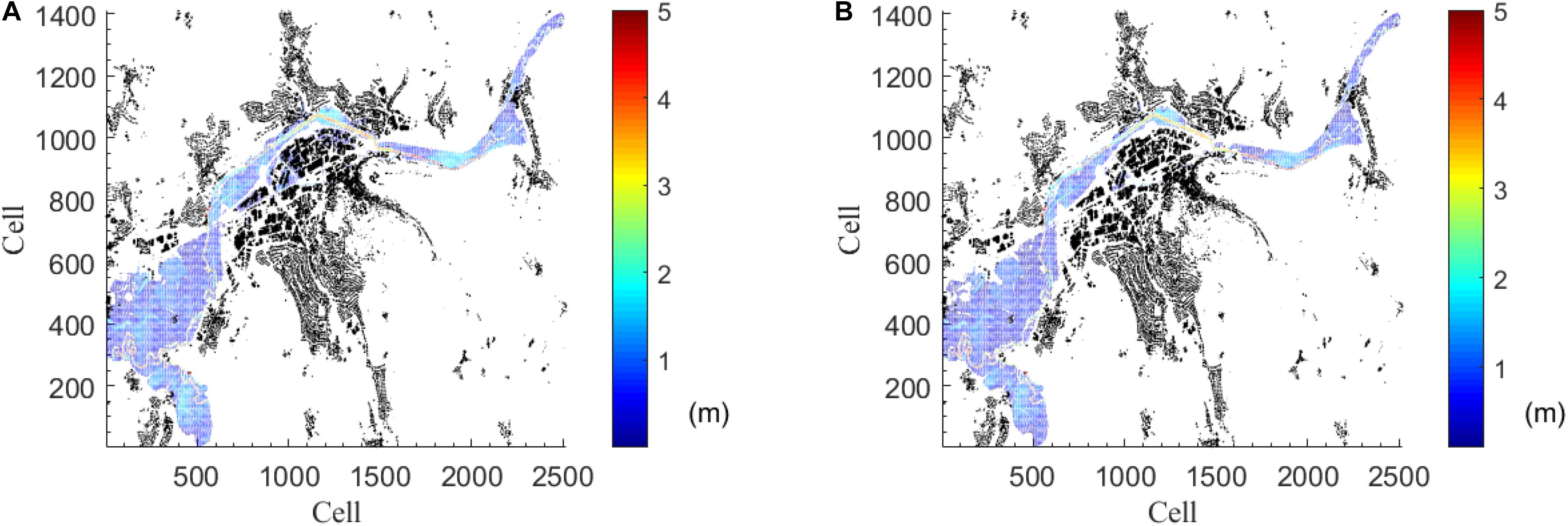
Figure 9. Example of flood inundation prediction in testing dataset (Event #180). Black parts are houses. (A) Inundation prediction from ANN model. (B) Inundation prediction from the database.

Prediction of Maximum Flood Inundation for Historical Events

The historical discharges from the historical events are taken from Bavarian Hydrological Services (Bhola et al., 2018). From the historical events, two representative events are selected to validate the ANN. The February 2005 is an example of an advective precipitation with lower peaks and longer duration, with an intensity of 2–3 mm/h. The May 2013 is an example of a convective precipitation with higher peaks and shorter duration, with an intensity of 5–60 mm/h.

Figures 10, 11 show the MSE obtained for the prediction of the historical event in February2005 and May 2013. In Figure 10, the large MSE occurs mainly in the ponding area to the southwest. Figure 11 shows larger MSE in the southwest than that in February 2005.

FIGURE 10

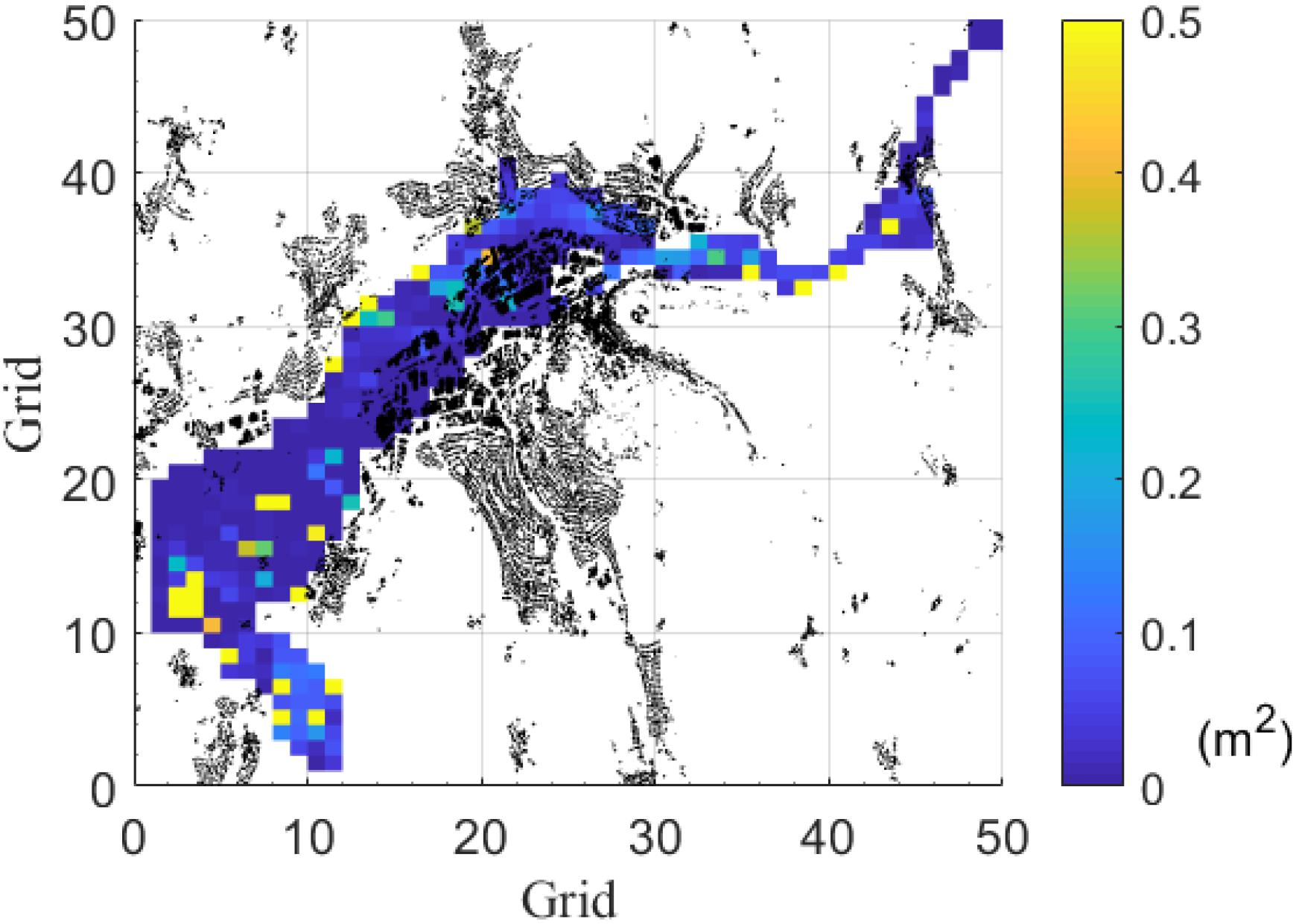
Figure 10. Average MSE difference between the ANN and the hydrodynamic model of the historical event in February 2005. Black elements are houses. Comparison of average MSE to observed inundation depth (historical event in February 2005). Each grid is an ANN.

FIGURE 11

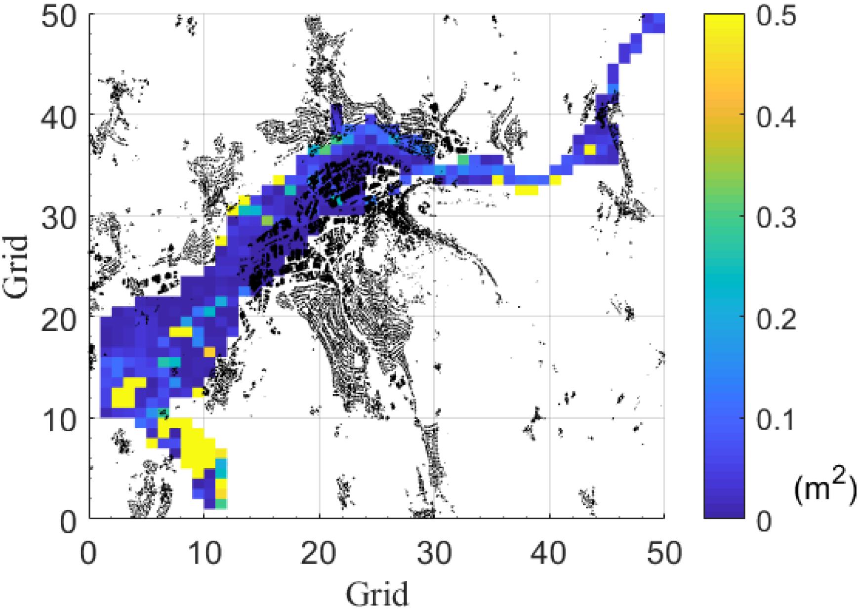
Figure 11. Average MSE difference between the ANN and the hydrodynamic model of the historical event in May 2013. Black parts are houses. Each grid is an ANN.

Discussion

Training Algorithm

In this section, the two training algorithms, resilient backpropagation and conjugate gradient are discussed. Figures 3, 4 support that both algorithms do not show overfitting. Indeed, similar MSE over the training dataset and the testing dataset are observed. However, we still observe a few grids, whose MSE has higher values, suggesting that increasing the size of the training datasets could further improve the performance. Figure 4 shows that the resilient backpropagation has a lower standard deviation of the MSE for the testing dataset compared to that of the conjugate gradient. As such resilient backpropagation is selected for as training algorithm. This is in line with other researchers which also described resilient backpropagation as efficient with forward-feed neural networks (Bustami et al., 2007; Chibueze and Nonyelum, 2009).

References

Abbot, J., and Marohasy, J. (2015). Improving monthly rainfall forecasts using artificial neural networks and single-month optimisation:a case study of the Brisbane catchment, Queensland, Australia. Water Resour. Manag. VIII 1, 3–13. doi: 10.2495/wrm150011
Berkhahn, S., Fuchs, L., and Neuweiler, I. (2019). An ensemble neural network model for real-time prediction of urban floods. J. Hydrol. 575, 743–754. doi: 10.1016/j.jhydrol.2019.05.066
Bermúdez, M., Cea, L., and Puertas, J. (2019). A rapid flood inundation model for hazard mapping based on least squares support vector machine regression. J. Flood Risk Manag. 12, 1–14. doi: 10.1111/jfr3.12522
Berz, G. (2001). Flood disasters: lessons from the past-worries for the future. Water Manag. 148, 57–58. doi: 10.1680/wama.148.1.57.40366
Bhola, P. K., Leandro, J., and Disse, M. (2018). Framework for offline flood inundation forecasts for two-dimensional hydrodynamic models. Geosci 8:346. doi: 10.3390/geosciences8090346
Bhola, P. K., Nair, B. B., Leandro, J., Rao, S. N., and Disse, M. (2019). Flood inundation forecasts using validation data generated with the assistance of computer vision. J. Hydroinformatics 21, 240–256. doi: 10.2166/hydro.2018.044
Bustami, R., Bessaih, N., Bong, C., and Suhaili, S. (2007). Artificial neural network for precipitation and water level predictions of bedup river. IAENG Int. J. Comput. Sci. 34, 228–233.
Chang, L. C., Amin, M. Z. M., Yang, S. N., and Chang, F. J. (2018). Building ANN-based regional multi-step-ahead flood inundation forecast models. Water (Switzerland) 10, 1–18. doi: 10.3390/W10091283
Chang, M. J., Chang, H. K., Chen, Y. C., Lin, G. F., Chen, P. A., Lai, J. S., et al. (2018). A support vector machine forecasting model for typhoon flood inundation mapping and early flood warning systems. Water (Switzerland) 10:734. doi: 10.3390/w10121734
Chibueze, T., and Nonyelum, F. (2009). Feed-forward neural networks for precipitation and river level prediction. Adv. Nat. Appl. Sci 3, 350–356.
Chu, H., Wu, W., Wang, Q. J., Nathan, R., and Wei, J. (2020). An ANN-based emulation modelling framework for flood inundation modelling: application, challenges and future directions. Environ. Model. Softw. 124:104587. doi: 10.1016/j.envsoft.2019.104587
Coulibaly, P., Anctil, F., and Bobée, B. (2000). Daily reservoir inflow forecasting using artificial neural networks with stopped training approach. J. Hydrol. 230, 244–257. doi: 10.1016/S0022-1694(00)00214-6
Dawson, C. W., and Wilby, R. L. (2001). Hydrological modelling using artificial neural networks. Prog. Phys. Geogr. 25, 80–108. doi: 10.1177/030913330102500104
Dineva, A., Várkonyi-Kóczy, A. R., and Tar, J. K. (2014). “Fuzzy expert system for automatic wavelet shrinkage procedure selection for noise suppression,” in Proceedings of the 2014 18th International Conference on Intelligent Engineering Systems, Tihany, 163–168. doi: 10.1109/INES.2014.6909361
Disse, M., Konnerth, I., Bhola, P. K., and Leandro, J. (2018). “Unsicherheitsabschätzung für die berechnung von dynamischen überschwemmungskarten – fallstudie kulmbach,” in Vorsorgender und Nachsorgender Hochwasserschutz: Ausgewählte Beiträge aus der Fachzeitschrift WasserWirtschaft Band 2, ed. S. Heimerl (Wiesbaden: Springer Fachmedien Wiesbaden), 350–357. doi: 10.1007/978-3-658-21839-3_50
Elsafi, S. H. (2014). Artificial neural networks (anns) for flood forecasting at dongola station in the river nile, sudan. Alexandria Eng. J. 53, 655–662. doi: 10.1016/j.aej.2014.06.010
Gizaw, M. S., and Gan, T. Y. (2016). Regional flood frequency analysis using support vector regression under historical and future climate. J. Hydrol. 538, 387–398. doi: 10.1016/j.jhydrol.2016.04.041
Hankin, B., Waller, S., Astle, G., and Kellagher, R. (2008). Mapping space for water: screening for urban flash flooding. J. Flood Risk Manag. 1, 13–22. doi: 10.1111/j.1753-318x.2008.00003.x
Henonin, J., Russo, B., Mark, O., and Gourbesville, P. (2013). Real-time urban flood forecasting and modelling–A state of the art. J. Hydroinformatics 15, 717–736. doi: 10.2166/hydro.2013.132
Humphrey, G. B., Gibbs, M. S., Dandy, G. C., and Maier, H. R. (2016). A hybrid approach to monthly streamflow forecasting: Integrating hydrological model outputs into a Bayesian artificial neural network. J. Hydrol. 540, 623–640. doi: 10.1016/j.jhydrol.2016.06.026
Kalyanapu, A. J., Shankar, S., Pardyjak, E. R., Judi, D. R., and Burian, S. J. (2011). Assessment of GPU computational enhancement to a 2D flood model. Environ. Model. Softw. 26, 1009–1016. doi: 10.1016/j.envsoft.2011.02.014
Kasiviswanathan, K. S., He, J., Sudheer, K. P., and Tay, J. H. (2016). Potential application of wavelet neural network ensemble to forecast streamflow for flood management. J. Hydrol. 536, 161–173. doi: 10.1016/j.jhydrol.2016.02.044
Kron, W. (2005). Flood risk = hazard values vulnerability. Water Int. 30, 58–68. doi: 10.1080/02508060508691837
Ludwig, K., and Bremicker, M. (eds). (2006). The Water Balance Model LARSIM: Design, Content and Applications. Germany: Institut für Hydrologie Universität Freiburg.
Mark, O., Weesakul, S., Apirumanekul, C., Aroonnet, S. B., and Djordjeviæ, S. (2004). Potential and limitations of 1D modelling of urban flooding. J. Hydrol. 299, 284–299. doi: 10.1016/j.jhydrol.2004.08.014
Marquardt, D. W. (1963). An algorithm for least-squares estimation of nonlinear parameters. J. Soc. Indust. Appl. Math. 11, 431–441. doi: 10.1017/CBO9781107415324.004
Mekanik, F., Imteaz, M. A., Gato-Trinidad, S., and Elmahdi, A. (2013). Multiple regression and artificial neural network for long-term rainfall forecasting using large scale climate modes. J. Hydrol. 503, 11–21. doi: 10.1016/j.jhydrol.2013.08.035
Mosavi, A., Ozturk, P., and Chau, K. W. (2018). Flood prediction using machine learning models: literature review. Water (Switzerland) 10, 1–40. doi: 10.3390/w10111536
Mukerji, A., Chatterjee, C., and Raghuwanshi, N. S. (2009). Flood forecasting using ANN, neuro-fuzzy, and neuro-GA models. J. Hydrol. Eng. 14, 647–652. doi: 10.1061/(asce)he.1943-5584.0000040
Nawi, N., Ransing, R., and Ransing, M. (2007). An improved conjugate gradient based learning algorithm for back propagation neural networks. Int. J. Comput. Intell. 4, 46–55.
Saini, L. M. (2008). Peak load forecasting using Bayesian regularization, Resilient and adaptive backpropagation learning based artificial neural networks. Electr. Power Syst. Res. 78, 1302–1310. doi: 10.1016/j.epsr.2007.11.003
Sit, M., and Demir, I. (2019). Decentralized flood forecasting using deep neural networks. arXiv. [Preprint]. arXiv:1902.02308.
Taghi, S. M., Yurekli, K., and Pal, M. (2012). Performance evaluation of artificial neural network approaches in forecasting reservoir inflow. Appl. Math. Model. 36, 2649–2657. doi: 10.1016/j.apm.2011.09.048
Taherei, G. P., Darvishi, H. H., Mosavi, A., Bin Wan, K., Yusof, K., Alizamir, M., et al. (2018). Sugarcane growth prediction based on meteorological parameters using extreme learning machine and artificial neural network. Eng. Appl. Comput. Fluid Mech. 12, 738–749. doi: 10.1080/19942060.2018.1526119
Thirumalaiah, D. (1998). River stage forecasting using artificial neural networks. J. Hydrol. Eng. 3, 26–32. doi: 10.1061/(asce)1084-0699(1998)3:1(26)
Tilson, L. V., Excell, P. S., and Green, R. J. (1988). A generalisation of the Fuzzy c-Means clustering algorithm. Remote Sensing 3, 1783–1784. doi: 10.1109/igarss.1988.569600
Tiwari, M. K., and Chatterjee, C. (2010). Development of an accurate and reliable hourly flood forecasting model using wavelet-bootstrap-ANN (WBANN) hybrid approach. J. Hydrol. 394, 458–470. doi: 10.1016/j.jhydrol.2010.10.001
Vogel, R. M., Yaindl, C., and Walter, M. (2011). Nonstationarity: flood magnification and recurrence reduction factors in the unitunited states. J. Am. Water Resour. Assoc. 47, 464–474. doi: 10.1111/j.1752-1688.2011.00541.x
Xu, S., and Chen, L. (2008). A novel approach for determining the optimal number of hidden layer neurons for FNN’s and its application in data mining. Conf. Inf. Technol. Appl. ICITA 2008, 683–686.
Yu, P. S., Chen, S. T., and Chang, I. F. (2006). Support vector regression for real-time flood stage forecasting. J. Hydrol. 328, 704–716. doi: 10.1016/j.jhydrol.2006.01.021
Keywords: hazard, maximum flood inundation extent, artificial neural network, resilient backpropagation, urban flood forecast
Citation: Lin Q, Leandro J, Wu W, Bhola P and Disse M (2020) Prediction of Maximum Flood Inundation Extents With Resilient Backpropagation Neural Network: Case Study of Kulmbach. Front. Earth Sci. 8:332. doi: 10.3389/feart.2020.00332
Received: 07 March 2020; Accepted: 17 July 2020;
Published: 05 August 2020.
Edited by:
Mingfu Guan, The University of Hong Kong, Hong KongReviewed by:
Huan-Feng Duan, Hong Kong Polytechnic University, Hong KongJiahong Liu, China Institute of Water Resources and Hydropower Research, China
Guangtao Fu, University of Exeter, United Kingdom
Copyright © 2020 Lin, Leandro, Wu, Bhola and Disse. This is an open-access article distributed under the terms of the Creative Commons Attribution License (CC BY). The use, distribution or reproduction in other forums is permitted, provided the original author(s) and the copyright owner(s) are credited and that the original publication in this journal is cited, in accordance with accepted academic practice. No use, distribution or reproduction is permitted which does not comply with these terms.
*Correspondence: Qing Lin, tsching.lin@tum.de