Prediction of Large Whale Distributions: A Comparison of Presence–Absence and Presence-Only Modeling Techniques

Introduction

Assessing the risk of anthropogenic activities on protected marine species requires quantitative and accurate representations of species distributions. Cetacean species distribution models have been used to predict the probability of cetacean presence, relative abundance or density throughout an area of interest and to gain insight into the ecological processes affecting these patterns (e.g., Redfern et al., 2006; Gregr et al., 2013). By fitting models of presence or abundance to relevant environmental variables, and then projecting them into geographic space, dynamic responses to environmental variability can be predicted (Becker et al., 2014, 2018). Predictions from these models can also be used to develop and evaluate management and conservation strategies (e.g., Redfern et al., 2013; McClellan et al., 2014).

Ideally, the data used in cetacean-habitat models would come from surveys designed to estimate cetacean abundance and distribution. Transect lines on this type of survey are positioned to ensure equal sampling probabilities throughout the study area or strata, and data include both sightings and effort. Conducting this type of survey is costly and such surveys have covered only a small fraction of the global oceanic habitat (Kaschner et al., 2012); most cetacean data are either from opportunistic sightings or non-systematic surveys of local areas. Consequently, using presence-only modeling techniques, which do not need observed absence or observer effort data, may expand our ability to conduct spatially explicit risk assessments for cetaceans.

The use of generalized additive models (GAMs) is common in species distribution modeling because it allows the data to identify non-linearities in species–habitat relationships rather than imposing parametric fits through polynomial terms in a linear regression (Chambers and Hastie, 1991). GAMs can predict presence/absence, the encounter rate of sightings, or the density of individuals when the data include observed zeros (absences). Maxent is a presence-only modeling technique that has been extensively applied and tested for terrestrial species (Phillips et al., 2006; Elith et al., 2011). Like the more commonly used technique of generalized additive modeling, it can fit complex relationships to environmental variables. The primary concern when using Maxent, as when using any presence-only modeling technique, is the spatial biases often exhibited in data that are not collected systematically (Dennis and Thomas, 2000; Guillera-Arroita et al., 2015). While incomplete sampling of species habitat can also occur in systematic surveys, biases in presence-only data collected without a systematic sampling design are much more pervasive. Presence-only data tend to be collected opportunistically in areas of known occurrence or areas that are easy to survey and they often encompass only a small portion of a species or population range. Measurements of effort are often missing from these data sets, making an assessment of spatial bias impossible.

Model comparison studies have shown that Maxent models using presence-only data are competitive with other presence-only and presence–absence methods for predicting species distributions, although most of this work has been in terrestrial systems (Elith et al., 2006; Shabani et al., 2016). We explored the performance of Maxent models using cetacean data from the eastern tropical Pacific. This is a large, well-surveyed area, with >300,000 km of systematically collected cetacean line-transect data and thousands of additional cetacean sightings collected opportunistically. NOAA Fisheries research vessel surveys have resulted in this region having the most cetacean line-transect survey effort in the world (Kaschner et al., 2012). Species distribution models have been successfully built for multiple species using the systematically collected survey data (Forney et al., 2012). Following a similar approach, we used the systematically collected data to develop GAMs for humpback (Megaptera novaeangliae), blue (Balaenoptera musculus), Bryde’s (Balaenoptera edeni), and sperm whales (Physeter macrocephalus). These species were selected because they represent a range of habitat selectivity from the narrow coastal distributions of humpback whales and regional centers of blue whale distributions to the broad distributions of Bryde’s and sperm whales.

In this study, we compare GAM and Maxent models, and we assess the performance of Maxent models that are based on data with varying levels of spatial bias. First, we compare GAM and Maxent models built with the same systematic survey data that include both presences and observed absences from the transect coverage, rather than the typical randomly selected background points or pseudo-absences for the Maxent models. The background data thus have the same potential spatial bias as the occurrence data (Phillips et al., 2009); this bias correction is not possible for strictly presence-only observations of occurrence. Second, we demonstrate spatial biases in presence-only Maxent model predictions arising from two sources: (1) the use of pseudo-absences randomly selected from climatological background data rather than the use of observed absences, and (2) spatial bias in observed presences from either opportunistic sampling or stratified systematic sampling with uneven coverage among strata. These analyses shed light on mechanisms of bias in Maxent models, using an extensive and unique marine survey data set.

Materials and Methods

Data Sources

The eastern tropical Pacific study area spans approximately 20 million km² of the Pacific Ocean and contains a diversity of habitat types and 30 species of cetaceans as residents (∼35% of currently recognized species; Ballance et al., 2006). We used cetacean and ecosystem assessment survey data collected by the National Marine Fisheries Service’s Southwest Fisheries Science Center (SWFSC) from August through November in 1986–1990, 1998–2000, 2003, and 2006. On all surveys, line-transect methods were used to collect marine mammal data during daylight hours (Kinzey et al., 2009) for a total of 302,381 km of search effort (Figure 1). These data are systematic, with rigorous recording of effort and sightings so that both presence and absence can be quantified. These systematic surveys were stratified to improve abundance estimates for endangered dolphin stocks (Gerrodette and Forcada, 2005); the intensity of yearly survey effort was increased by a factor ranging from 1.24 to 3.38 (mean 2.34) within a core area (Figure 1). We also used whale sightings collected opportunistically, without associated effort or environmental data, during July–November 1980–2010. These data are available in SIBIMAP¹, a regional database that provides compiled and standardized cetacean data from a variety of sources in the eastern Pacific Ocean. We excluded SWFSC systematic sightings that are included in the SIBIMAP opportunistic records.

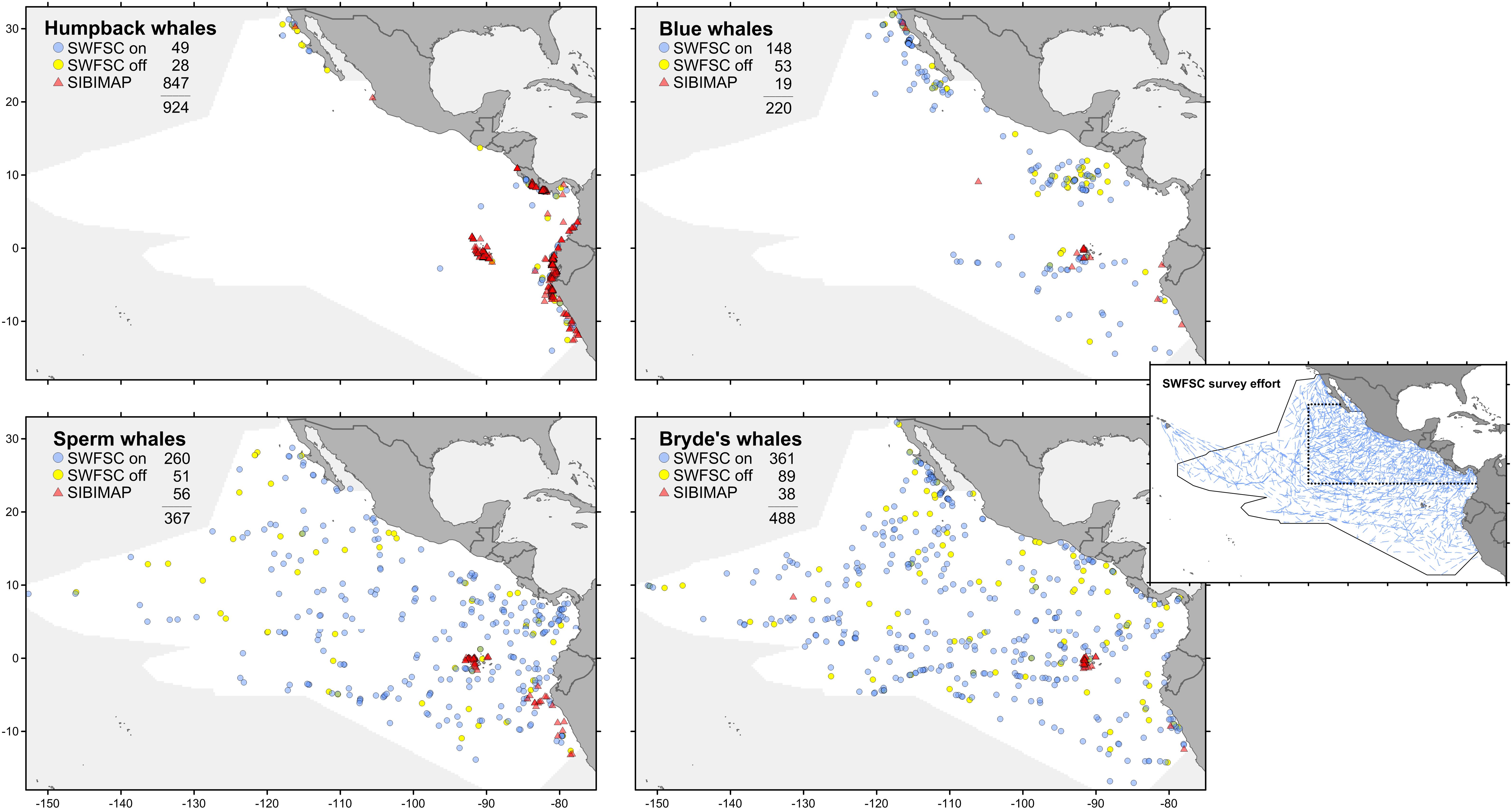
FIGURE 1. Sighting locations for four whale species from systematic surveys (see text for explanation of on-effort and off-effort) and opportunistic records (presence-only). All sightings are July–November. Stratified survey on-effort tracklines (inset): dotted line is the core survey area, which has greater coverage than the outer stratum; solid line is the survey study area.

Five environmental variables were used as predictors: surface temperature, surface salinity, thermocline depth, stratification index, and distance to shelf edge. These variables represent surface water mass identity, physical processes such as mixing and upwelling, and bathymetric features that influence prey availability. For each of these, the same variable or a related variable, e.g., mixed layer depth rather than thermocline depth, has been found to be important as a predictor variable in the eastern tropical Pacific or other regions (Forney et al., 2012; Becker et al., 2017).

An ocean reanalysis combines oceanographic observations with a general ocean model to produce estimates of variables describing the changing state of the ocean in time and space; the observations correct biases in the model, while the model fills in gaps between the assimilated observations (Balmaseda et al., 2015). We used ocean reanalysis data to estimate the four dynamic environmental variables: sea surface temperature and salinity, thermocline depth, and stratification index (Figure 2). Data values for sightings or systematic effort segments were spline-interpolated from year–month composites of six ocean reanalysis data sets as described in Fiedler et al. (2017). The thermocline was considered to be the depth interval that included the upper decile (the greatest 10%) of 1 m temperature gradients in a 0–300 m temperature profile. Thermocline depth is the weighted mean of the depths of this set, with each depth weighted by the value of the 1 m temperature gradient at that depth. Stratification index is the standard deviation of temperature in the near-surface layer, 0–300 m (Fiedler, 2010). A fifth environmental variable, distance to the edge of the continental shelf, was derived from the geomorphic features map (GSFM) of the global ocean (Harris et al., 2014). Correlations among these variables are in Table 1.

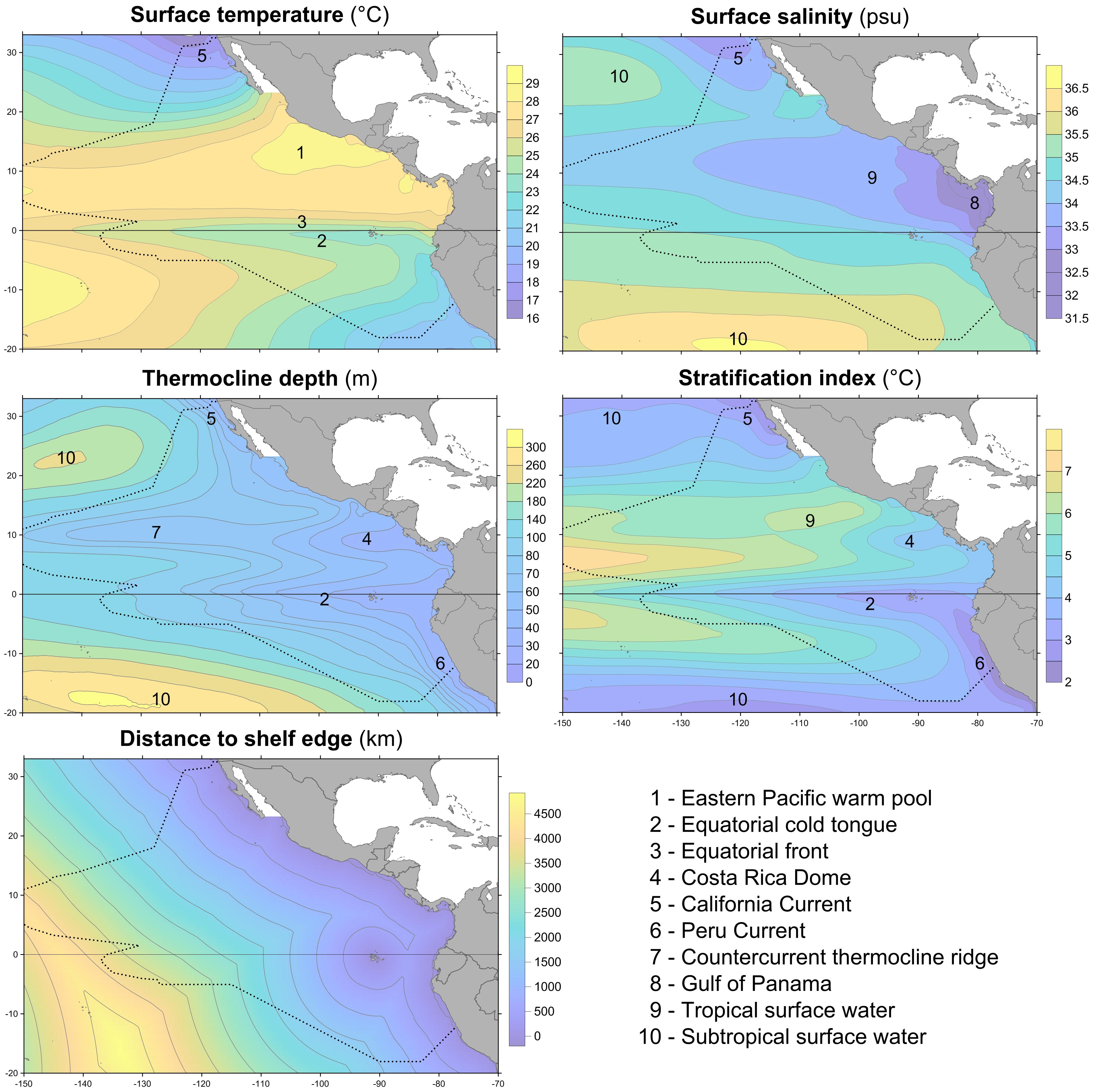
FIGURE 2. Climatologies of predictor variables (1980–2015) and important environmental features in the eastern tropical Pacific. Dotted line is the survey and model study area.

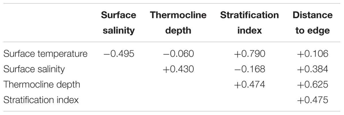
TABLE 1. Correlation matrix for predictor variables in SWFSC survey segments (n = 33,229).

Species distribution models were built for each of the four large whale species: humpback, blue, sperm, and Bryde’s whales. Sightings from systematic surveys and opportunistic records are plotted in Figure 1. The systematic sightings were divided into two categories: on-effort sightings are those made while observers were on effort, but excluding sightings not used for abundance estimation (>5.5 km perpendicular distance from the trackline or made by the independent observer); off-effort sightings are all other sightings made by any observer not engaged in active searching, such as on a chase to identify an on-effort sighting. The survey trackline segment data used for GAM contain only on-effort sightings. Prevalence (fraction of 1° squares in the study area occupied by at least one sighting) increases as follows: humpback whale 0.036, blue whale 0.057, sperm whale 0.120, Bryde’s whale 0.159. For comparison, the prevalence of SWFSC survey trackline segments is 0.661. The sampling bias of the opportunistic records for all species is readily apparent in Figure 1; nearly all of these sightings are in limited near-coastal areas.

In addition to sampling bias, there are two other sources of error that can influence species distribution models: detection bias and occupancy bias (Yackulic et al., 2013). We assume that both the systematic and opportunistic sightings data are subject to the same detection bias. Systematic survey effort is suspended at sea states greater than Beaufort 5 and under low visibility conditions. Presumably, opportunistic sighting effort would be similarly constrained. Occupancy bias affects any prediction of the distribution of rare species; only a small fraction of the area predicted as suitable for presence will actually be occupied. We assume that this bias will be equivalent for Maxent and GAM model predictions. Although we ignore potential occupancy and detection biases to focus on sampling bias for this comparative study, these biases may need to be addressed in other applications.

Variable values for each sighting or effort segment were extracted from the ocean reanalysis data corresponding to the year and month, and 0.25° grid square, of the observation. Thus, we did not use climatological data for the models. Model resolution was 0.25° latitude/longitude. This resolution was selected to allow effective alignment of the ocean reanalysis data grids.

Model Comparisons

We performed four sets of model comparisons, with each of the four whale species, to (1) compare Maxent and GAM modeling using the same presence–absence data, and (2–4) explore changes in Maxent model predictions that arise from spatial biases in the distribution of presences and the selection of pseudo-absences:

(1) Maxent and GAM with observed absences. To compare Maxent to GAM models using the same presence and absence data, we built “observed-absence” Maxent models with systematic survey on-effort sightings and background data points selected from survey effort segments that had no sightings of the modeled species.

(2) Maxent with observed and pseudo-absences. Maxent conventionally uses presence-only data and pseudo-absences. To assess the effect of using pseudo-absences for presence-only modeling, we compared the “observed-absence” Maxent models to “presence-only” (pseudo-absence) Maxent models built by the usual method that randomly selects pseudo-absences from background cells that do not contain observed presences.

(3) Maxent spatial bias of opportunistic samples. To assess the effects of the spatial bias in opportunistic samples on Maxent predictions, we built presence-only Maxent models with opportunistic records alone and combined with systematic survey sightings. These model predictions were compared to the presence-only Maxent models built with the systematic survey sightings.

(4) Maxent spatial bias of stratified systematic samples. To assess the effects of the spatial bias in stratified, non-uniform systematic survey data on Maxent predictions, we built presence-only Maxent models with systematic survey sightings that were subsampled to correct for the increased effort in the core area. These model predictions were compared to the “presence-only” Maxent models built with all of the systematic sightings.

Modeling

We applied GAMs to the systematically collected on-effort data to predict presence from the environmental variables. Survey transects were divided into continuous-effort segments of approximately 10 km as described by Becker et al. (2010) and Forney et al. (2012). Almost all of these segments were observed absences (effort but no sightings). We converted the segment data to presence–absence by assigning a value of 1 to the segments with 1 or more sightings. We fit Binomial GAMs with a logit link using the R (version 3.4.0; R Core Team, 2017) package mgcv (version 1.8-4; Wood, 2011). The distance traveled on effort in each segment was added as a covariate in the models to account for variations in segment length. We allowed a maximum of three degrees of freedom for each spline to limit over-fitting (Becker et al., 2014) and thus facilitate comparison between GAM and Maxent models.

Maxent was applied to the systematic survey sightings data and to the opportunistic records to predict probability of presence from the environmental variables (Phillips et al., 2017). Maxent modeling was performed using the Maximum Entropy Species Distribution Modeling software, v. 3.4.1², run using the R package “dismo,” v. 1.1-4³. A regularization multiplier of 2 was used to limit over-fitting. Too much flexibility in model fitting, either by excessive degrees of freedom in GAM or minimal regularization in Maxent, can make it hard to differentiate noise from real species-response signals in a data set (Merow et al., 2013). Sightings, with corresponding environmental variable values, were input to Maxent in SWD (samples-with-data) format files. Duplicate presence records, in 0.25° background cells (n = 29,371 cells), were not removed. Whales are motile and the marine environment is dynamic; sightings that are coincident in space but separated in time will be associated with different environmental conditions. To simplify model comparison, neither Maxent product features nor GAM interaction terms were used. Maxent threshold features were also not used (Phillips et al., 2017). The number of randomly selected background points was set at 1,000 to be comparable to the numbers of observed presences (29–865 sightings). Fifty replicate model predictions were generated with randomly selected background points and then averaged. Finally, the default option “Add samples to background” was retained. We found that Maxent did not perform well when presence samples had environmental variable values outside the range of background values that are taken from the ocean reanalysis grids.

Model Assessment

Species distribution models are commonly assessed by AUC, but its utility has been questioned for several reasons (Lobo et al., 2008; Araújo and Peterson, 2012; Golicher et al., 2012; Jiménez-Valverde, 2012). The main issues are that AUC (1) does not reflect the goodness-of-fit of the model predictions or the spatial distribution of model errors, and (2) is not theoretically valid for evaluations of presence-only models built by using background data as pseudo-absences. To assess goodness-of-fit (issue 1), we also report point biserial correlation (COR) between observed presence/absence (1 or 0) and model predictions in the corresponding model cells (Elith et al., 2006). Spatial distributions of model errors are illustrated by maps of differences between compared model predictions. Difference maps were calculated after standardization of the log-transformed predictions, because of the different scalings of the model predictions. We tested the effect of the violation of AUC theory caused by using background pseudo-absences (issue 2) by comparing evaluations of Maxent models built with observed absences and with pseudo-absences.

Performance metrics for all models were calculated with a set of both on- and off-effort systematic sightings, subsampled within the core survey area as described above, and with duplicate sightings in the same 0.25° cell removed. Although these samples are not independent of the presences used to build the models based on systematic on-effort sightings, we consider these sightings to be the most complete and unbiased sample of the true distribution of the four whale species in the study area. All Maxent and GAM model predictions were assessed with 1,000 bootstrap replications of 1,000 randomly selected cells or segments as absences. AUC and COR were calculated using “evaluate” in the R package “dismo,” v. 1.1-4 (see footnote 3). Since the only source of variation in performance metric values for a model was the 1,000 bootstrap replications, significant differences between AUC or COR values were tested conservatively by non-overlap of mean ± SD intervals.

The relative importance or contribution of predictor variables to a model prediction was estimated as in Thuiller et al. (2009) to facilitate comparison between models. For a given Maxent model or GAM, each of the five variables was randomly permuted before being used to calculate a prediction surface. The correlation of the original prediction with the prediction using a permuted variable is related to the importance of the permuted variable: permuting an unimportant variable will change the prediction only slightly and result in a high correlation, while permuting an important variable will result in more change in the prediction and a lower correlation. The scores of variable importance are equal to 1 minus the correlation, rescaled to sum to one across all predictor variables.

Results

Maxent and GAM With Observed Absences

The two modeling methods produce very similar predictions from the same set of systematic presence/absence data (Figure 3). Pearson’s correlations between the GAM and Maxent model prediction cell values are: humpback whales +0.813, blue whales +0.900, sperm whales +0.831, and Bryde’s whales +0.888. The overall shapes of the prediction surfaces are visually similar, although there are minor discrepancies as shown in the difference maps. The performance metrics for the Maxent and GAM predictions are significantly different only for the more prevalent sperm and Bryde’s whales (Table 2).

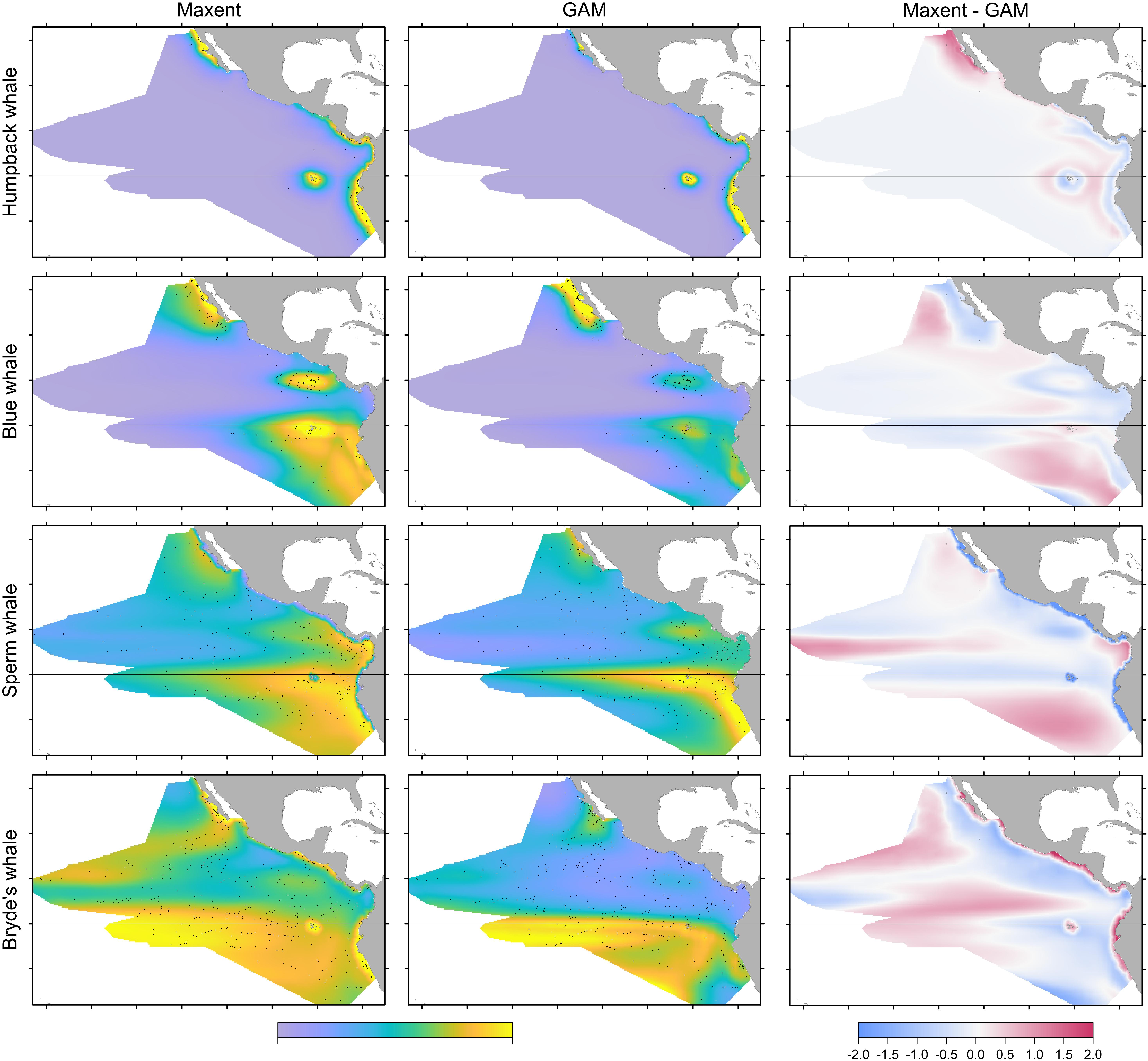
FIGURE 3. Comparison of predictions for Maxent and GAM models built with stratified survey presences and absences. In the first two columns, the prediction values range between 0 and 1, but the central tendencies are different for Maxent and GAM. The sightings included in the maps are both on-effort and off-effort (). For the difference maps (right column), the prediction values were log-transformed and standardized prior to differencing (see text).

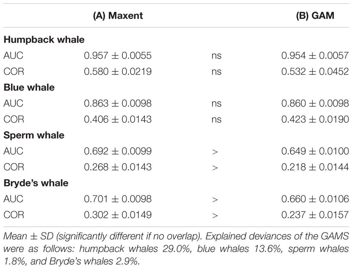
TABLE 2. Performance metrics for (A) Maxent and (B) GAM models, both built with observed presences and absences from systematic survey effort segments.

Humpback whale predicted presence is high along the coasts of Baja California and from Central America to the south, and around the Galapagos. The difference map shows that Maxent tends to emphasize the Baja California coastal high (red). Blue and red bands aligned with the edges of prediction highs indicate differences in the amplitude and extent of the highs, in this case off Central and South America and the Galapagos. Distance to shelf edge was an important predictor in both models, but was dominant for Maxent (Table 3).

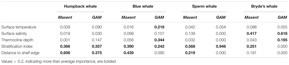
TABLE 3. Relative importance of variables in Maxent models and GAMs built with systematic survey segment presences and absences.

Blue whale predicted presence is high in the California Current along Baja California, at the Costa Rica Dome, near the equator centered at the Galapagos, and off the coast of Peru. Although the same highs are predicted by both models, the difference map shows differences in amplitudes and spatial extents throughout the study area, except in the far west.

Sperm and Bryde’s whales had lower correlations between Maxent and GAM predictions, but the GAMs had very low explained deviances for these more prevalent species. Sperm whale predicted presence in both models is moderately high off Baja California, and in the eastern equatorial Pacific (8°S–12°N) with highest values at the Costa Rica Dome, along the equator, in the Gulf of Panama, and along the Peru coast. These highs are attributable to the predominant influence of stratification index on the model predictions (Table 3). The difference map shows that the GAM predictions are higher at the Costa Rica Dome and along the equator, while the Maxent predictions are higher in the Gulf of Panama. Maxent used distance to shelf edge to predict lower probability of presence on the continental shelf.

Bryde’s whale predicted presence is high along the equator and to the south, along the coast of southern Baja California and extending to the southwest, and at the Costa Rica Dome. Both models predict low presence in the eastern Pacific warm pool off southern Mexico. The GAM emphasizes the Costa Rica Dome high, while Maxent emphasizes the presence of these whales in near-coastal areas. Salinity is the most important predictor in both models.

Maxent With Observed and Pseudo-Absences

Building Maxent models using background pseudo-absences with climatological predictor variable values resulted in different predictions, compared to the Maxent models built with observed absences that were shown in Figure 3. The difference maps show a similar pattern for all species, although the intensity of the pattern increases markedly with prevalence (Figure 4). Performance metrics also changed, depending on prevalence (compare columns B and C in Table 4). For the less prevalent species (humpback and blue whales), AUC and COR increased when models were built and evaluated with pseudo-absences, but decreased for Bryde’s whale models, with no change for sperm whales. Table 4 also shows that for Maxent models built with pseudo-absences or with observed absences, the performance metrics tend to be higher when the same type of absences are used in calculating AUC and COR (column B compared to A, and column C compared to D). However, these differences were not significant for humpback whales and significance increases were observed only for the more prevalent whales.

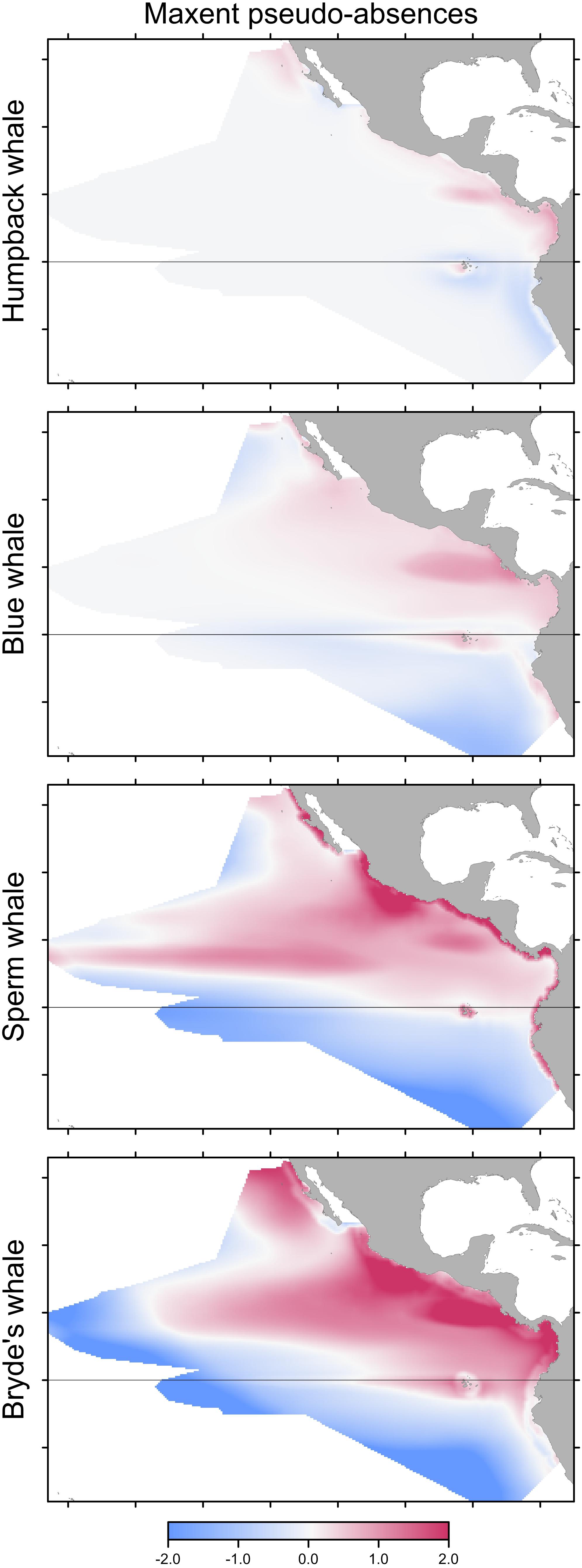
FIGURE 4. Differences between predictions of Maxent models built with pseudo-absences and with observed absences. Differencing as in Figure 3: red indicates that the pseudo-absence model prediction is greater than the observed absence model prediction.

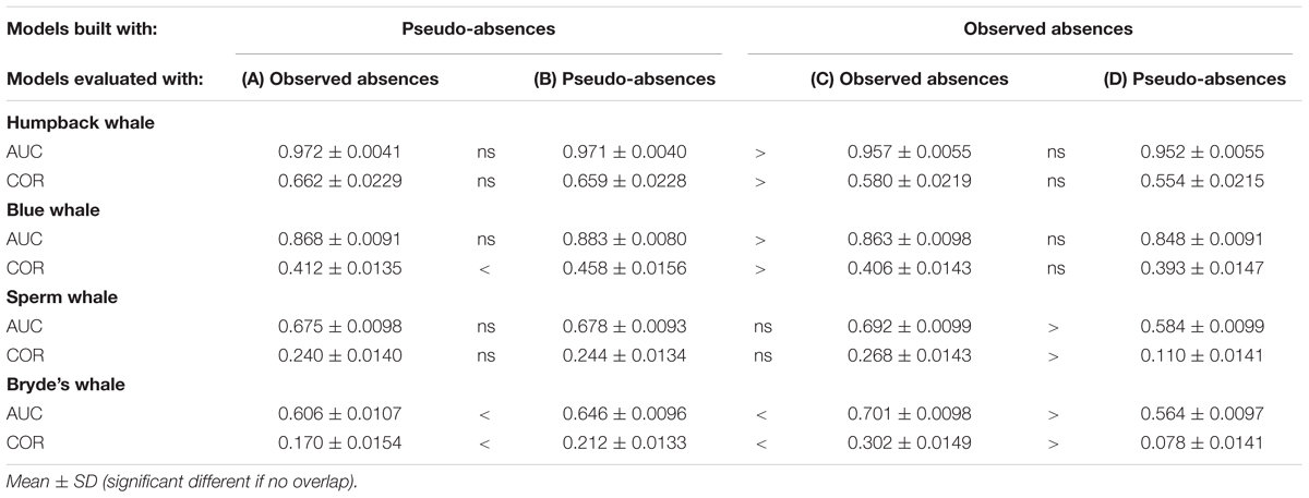
TABLE 4. Performance metrics of Maxent models built with systematic survey sightings, using observed absences and pseudo-absences for model building and/or for model evaluation.

Maxent Spatial Bias of Opportunistic Samples

Predicted distributions from Maxent models built with opportunistic records differed from those of models built with systematic survey sightings, as shown by the difference maps in the left column of Figure 5. Differences increased with prevalence, reflecting the increasing discordance of the spatial distributions of the opportunistic and systematic sightings shown in Figure 1. The Pearson correlations between the Maxent model prediction cell values based on the two data sets are: humpback whales +0.931, blue whales +0.744, sperm whales +0.352, and Bryde’s whales +0.270. For blue, sperm and Bryde’s whales, the predicted probabilities of presence are either reduced or elevated where there were no opportunistic sightings, while the prediction bias is strongly positive where the opportunistic sightings are located, around the Galapagos and along the coast of Peru. The effect of this bias is small for humpback whales, because the numerous opportunistic records were all on or near the coast and sightings from the systematic surveys also occurred along the coast, although they tended to be more offshore.

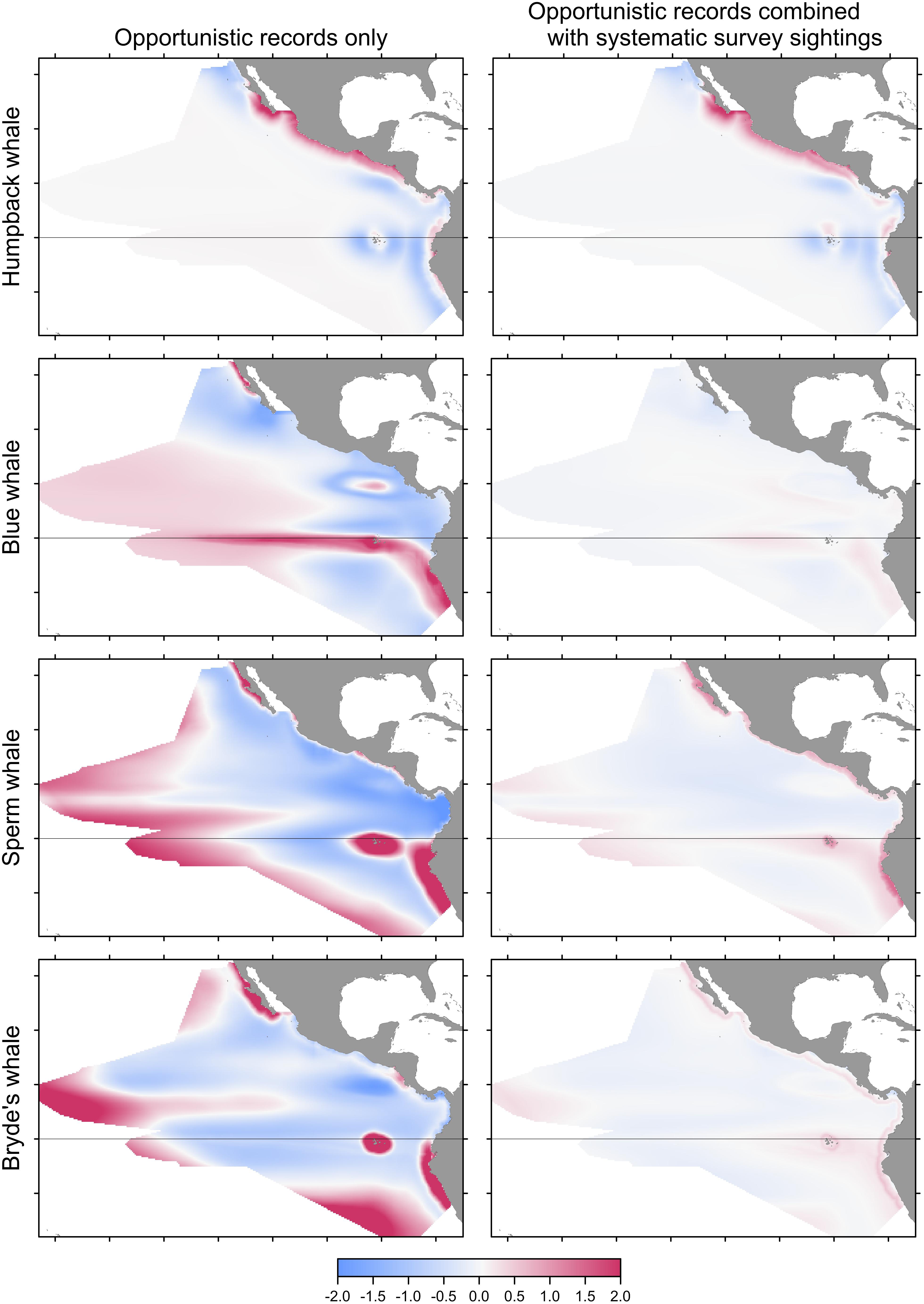
FIGURE 5. Bias or change in predictions of Maxent models built with pseudo-absences if opportunistic records are used alone (left) or combined with the systematic sightings (right). Differencing as in Figure 3: red indicates that the opportunistic records result in a higher predicted probability of presence.

For all species, the performance metrics decreased for Maxent models built with opportunistic records, although the differences were statistically significant only for sperm and Bryde’s whales (Table 5, columns A and B). When the opportunistic records are combined with the systematic survey sightings, the spatial biases are much less pronounced, as shown by the difference maps in the right column of Figure 6.

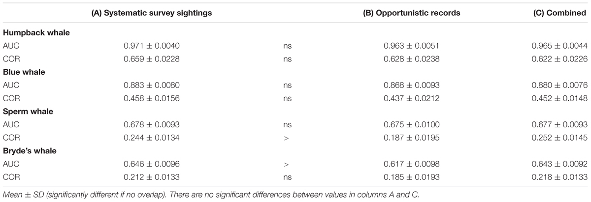
TABLE 5. Performance metrics of Maxent models built with (A) systematic survey sightings, (B) opportunistic records, and (C) a combination of opportunistic records and systematic survey sightings.

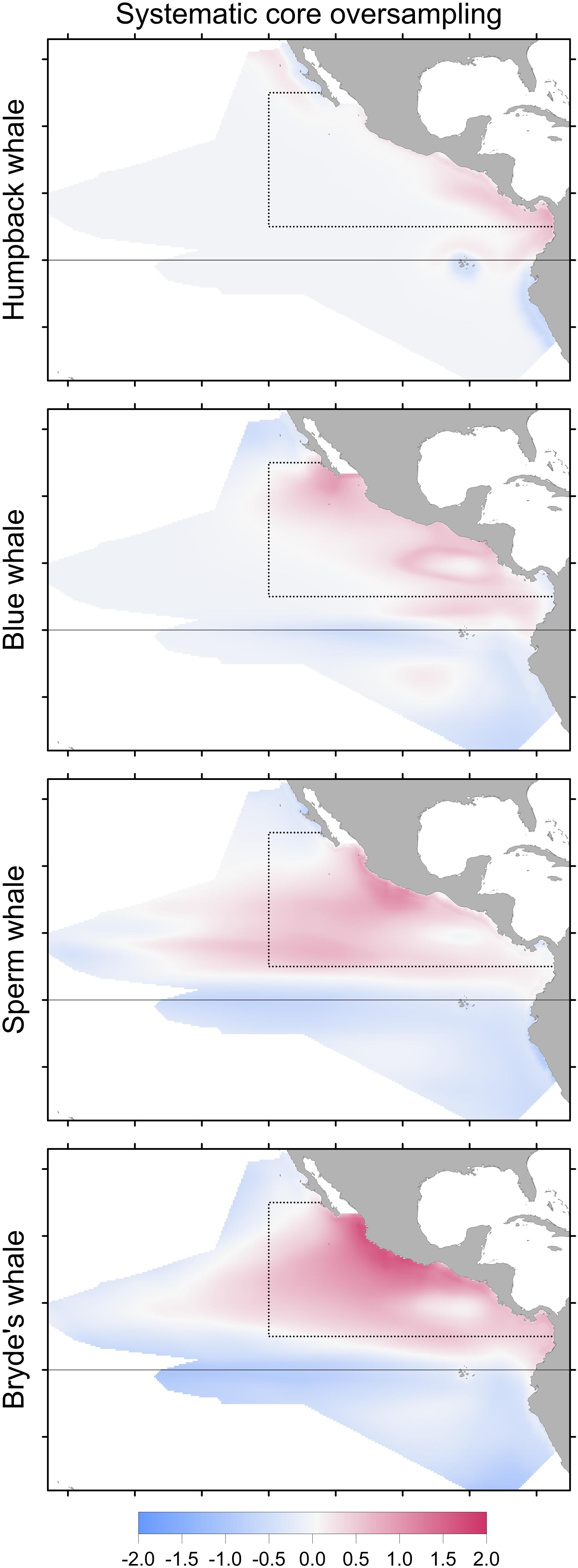
FIGURE 6. Change in Maxent predictions if stratified survey bias is corrected by subsampling the systematic sightings in the core area (dotted line), compared to the model built with systematic sightings without correcting for stratified oversampling in the core area. Differencing as in Figure 3: red indicates that no correction results in a higher predicted probability of presence.

Maxent Spatial Bias of Stratified Systematic Samples

Stratified systematic sampling is not uniform; the resulting sampling bias affects Maxent model predictions. When oversampling in the core area stratum is corrected, prediction levels are reduced in the core area for all species in the difference maps (Figure 6). However, the model performance metrics do not change significantly (Table 6).

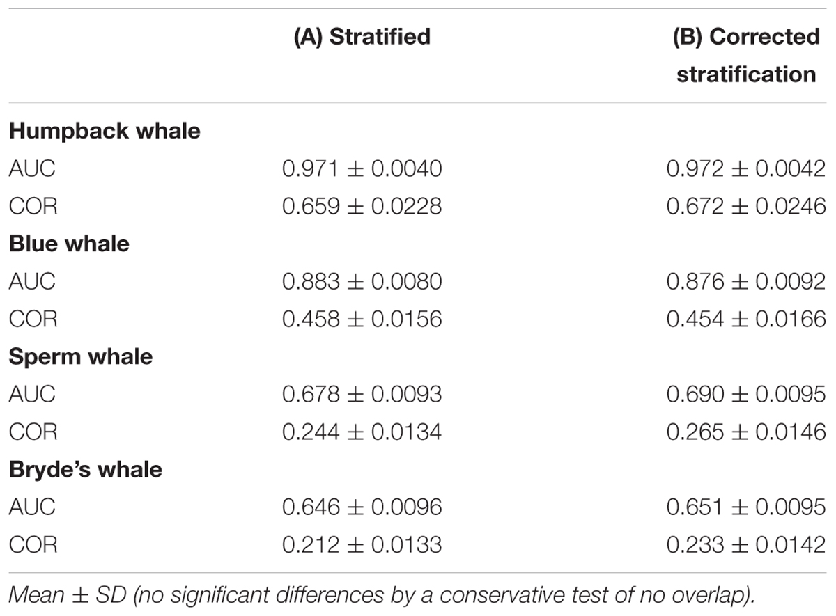
TABLE 6. Performance metrics of Maxent models built with (A) systematic survey sightings and (B) systematic survey sightings corrected for stratified oversampling in the core area.

Discussion

Two fundamentally different methods of species distribution modeling, GAM and Maxent, were used to generate model predictions for four species of large whales in the eastern tropical Pacific Ocean. One of the primary reasons for Maxent’s popularity and widespread application in recent years is its ability to make use of presence-only data. These data are less expensive to collect and therefore offer larger sample sizes than systematic data, as discussed by Elith and Leathwick (2009). Maxent presence-only predictions have been shown to be generally similar to predictions from presence–absence models for terrestrial data sets (Elith et al., 2006), and more recently for marine species (Sundblad et al., 2013). In general, our GAMs and Maxent models showed some similarities and some differences in geographical space (Figure 3). We found that Maxent can produce models similar to GAM presence–absence models only if background data points are selected from observed absences (see the section “Maxent and GAM With Observed Absences”). Tobeña et al. (2016) used Maxent to model cetacean distributions from fisheries observer program data; they treated sightings as presence-only data, but used trackline data to select pseudo-absences to correct for sampling bias (Phillips et al., 2009). We showed that this practice corrects bias caused by random pseudo-absences, but it is not possible with a strictly presence-only data set.

Maxent Prediction Biases

Although our results suggest that Maxent can produce species distribution models that are similar to GAMs (comparison 1), they also show that the use of random pseudo-absences alters Maxent predicted distributions (comparison 2). When systematic presence-only data were modeled with pseudo-absences in Maxent, the spatial pattern of predictions was considerably altered compared to Maxent models built with observed presence and absence data (Figure 4). Our performance metrics, AUC and COR, were also influenced by whether observed or pseudo-absences were used for model evaluation. A modeler should be aware of the influence of pseudo-absences on presence-only Maxent modeling even before the effects of sampling bias are considered (comparisons 3 and 4).

Many authors have found that AUC does not adequately measure the accuracy of a model prediction relative to observed presences. There are many other indices of model performance or accuracy that might be more appropriate for certain purposes (Hirzel et al., 2006). We show that spatial maps of differences between models can show important differences that are not apparent in comparisons of either AUC or COR performance metrics. Comparison of presence-only models based on metrics such as AUC and COR should consider the effects of how the absences are selected for calculating the metrics used for evaluation. Maxent AUC values are lower for more prevalent, widely distributed species (Phillips et al., 2006), as in our results. Lobo et al. (2008) show how AUC is affected by the distributions of both absences and presences within the range over which the model extends. Relying on AUC by default, may give misleading results when assessing or comparing models of species distributions.

The sampling bias of presence-only data, like our opportunistic cetacean sightings data, can result in misleading model predictions (Syfert et al., 2013). Maxent models built only with opportunistic records resulted in greatly altered prediction levels (probability of presence), with both positive and negative errors (Figure 5). Because the models are formulated in niche space, the biases introduced by opportunistic sampling extend throughout the study area when the model is projected in geographic space. When we tried using a combined data set of systematic survey sightings plus opportunistic records, the spatial biases in Maxent model predictions were reduced, but still apparent. Predictions tended to be less biased for humpback whales, even though there were many more opportunistic sightings than systematic sightings, because the opportunistic sightings occurred in the near-coastal preferred habitat of this species. For rare, data-limited marine species such as large whales, it is tempting to use opportunistically collected sightings data when the provision of management advice is hindered by small sample sizes. However, even if opportunistic data are added to a systematic data set, to fill in gaps in time and/or space, sampling bias must be considered if the study area is not adequately covered by the sampling effort.

Maxent offers two options to account for spatial bias in presence-only samples (Phillips et al., 2009; Merow et al., 2013). The first is to input a “bias grid” which is then used to correct for the specified sampling bias. The bias grid gives a priori relative sampling probabilities, thus modeling starts with a biased prior rather than a uniform prior for geographical distribution. This option is only available in the Maxent software if the environmental data are input from grids. In this study, a biased prior could not be specified because environmental variable values that were contemporaneous with the sightings were input in the SWD file. Maxent was developed to take advantage of presence-only data from specimens in museum collections and historical records of occurrences of terrestrial plants and animals (Phillips et al., 2006), for which environmental data from climatological background grids can be more reasonably utilized than in the dynamic ocean environment.

The second option to account for spatial sampling bias in Maxent models is to limit the coverage of background cells to the area sampled, i.e., the biased background approach (Merow et al., 2013). This is similar to what we did when we built observed-absence Maxent models by selecting pseudo-absences from survey trackline data. For presence-only modeling in the Maxent software, the background cells with environmental data can be input in the same type of file (SWD) as the sightings and their associated environmental data. We found that when this method of correcting for the coastal spatial bias of opportunistic samples was applied to our more prevalent, and thus more spatially biased, species (blue, sperm and Bryde’s whales), the extrapolation in environmental space required to cover the unsampled study area resulted in poor model predictions (not shown). An alternative is to correct for positive bias in oversampled areas, as we did to correct the uneven sampling in SWFSC stratified systematic survey data. Fourcade et al. (2014) also found that systematic subsampling of spatially biased observed presences was an effective way to correct this bias. However, for severely biased samples such as our SIBIMAP opportunistic records, this procedure reduces sample size and cannot effectively correct for absence of sampling in large parts of the study area.

Do the Models Make Ecological Sense?

Model performance, in the sense of verifying model predictions, can also be assessed subjectively in relation to existing knowledge. Specifically, we can consider whether our model predictions are consistent with what we know about the biology and ecology of the species. The less-prevalent species, humpback whales and blue whales, are seasonal migrators thought to be present in the warm eastern tropical Pacific during the winter months of the hemisphere where they feed in productive high-latitude waters. In general, seasonally migrating whales move to lower latitudes during the winter for breeding and, possibly, for predator avoidance or energetic savings related to calf survival (Corkeron and Connor, 1999; Rasmussen et al., 2007; Stern and Friedlaender, 2018). The humpback whales sighted along the coast of tropical Central and South America and at the Galapagos during the SWFSC systematic surveys were on known calving grounds and were most likely southern-hemisphere whales (Rasmussen et al., 2007; Félix et al., 2011). The whales along Baja California at the northern extreme of the study area, however, were probably northern-hemisphere whales on their summer feeding grounds. Overall, humpback whale predicted presence was higher in shallow coastal habitat, which is relatively cool and productive. Habitat preferences are likely different during migration. However, the Peru coastal waters where predicted presence is also high, are a seasonal migration corridor for humpback whales (Félix and Guzmán, 2014).

The blue whales observed in the eastern tropical Pacific during July–November include North Pacific whales on their feeding grounds off southern Baja California, whales at the Costa Rica Dome that are residents and/or South Pacific whales on their calving grounds and opportunistically feeding, and South Pacific whales to the west and south of the Galapagos that are calving and/or opportunistically feeding (Palacios, 1999; Sears and Perrin, 2018). Blue whale predicted presence was higher in waters with a shallow thermocline, which were also relatively cool and moderately stratified. Surface waters in the eastern tropical Pacific are stratified year-round, so a shallow thermocline indicates upwelling and higher nutrient availability for primary production (Fiedler and Talley, 2006). Blue whales occurring near the Costa Rica Dome, along Baja California, and in the vicinity of the equatorial cold tongue could have been feeding on euphausiid prey (Reilly and Thayer, 1990; Hoyt, 2009). The Maxent model and GAM had mixed success in predicting the presence of blue whales in the southeast Pacific extending from Chile (beyond the study area) to the equator. Connections between blue whales feeding off Chile and near the Galapagos (likely breeding) have recently been established (Buchan et al., 2015; Torres-Florez et al., 2015).

The more prevalent species in our study area, sperm whales and Bryde’s whales, are known to be widely distributed. Sperm whales, the only toothed whale of the four studied here, consume a variety of meso- and bathypelagic squids and fishes. The whales observed in the eastern tropical Pacific were most likely females and young males; adult males feed at higher latitudes in both hemispheres (Whitehead, 2009).

Bryde’s whales are one of the least well known species of large baleen whales and taxonomic uncertainties remain (Kato and Perrin, 2018). This species or species complex is widely distributed in tropical and temperate waters of all the world’s oceans, feeding on schooling pelagic fishes, and may migrate toward the equator in winter and to higher latitudes in summer. Species distribution or niche modeling may be difficult for such an ambiguous taxon, but could also yield insights into niche separation if the different taxonomic groups have distinct environmental preferences.

The model comparisons that we used to illustrate both the biases and the potential utility of Maxent are limited to the species and area for which we had exceptional systematic survey data. The results might be different for other organisms or environments. Even if sampling bias is adequately corrected in applying Maxent, this technique can only estimate patterns of presence or occurrence. For some purposes, the ability of GAMs to predict density or abundances may be essential. For example, estimates of the number of animals impacted by human activities are required by United States federal regulations.

A multitude of possible predictor variables could be used to describe the habitat of the whale species modeled in this study. Some variables might be more ecologically plausible, such as density or availability of prey organisms, but estimates of such variables are very difficult to obtain and are rarely available. Modelers commonly assume that the available oceanographic predictor variables will serve as proxies for prey. The direct use of forage or prey availability as predictors of marine top predator distributions is a recent approach (Stewart et al., 2014; Boyd et al., 2015; Zerbini et al., 2015). Studies of predator–prey relationships on spatial and temporal scales finer than the present study may benefit from concurrent observations of both predator and prey organisms, although Torres et al. (2008) showed that predictions of bottlenose dolphin distributions in a heterogeneous coastal habitat can be made without relying on prey data as explanatory variables. On larger scales, prey data from ocean ecosystem models promises to be useful in future cetacean prediction models (Lambert et al., 2014).

Conclusion

Predictions of species distributions from GAMs are valuable management tools. Both the presence–absence GAMs and Maxent models of large whale distributions presented here are useful in understanding the spatial distribution of these species and predicting distributions from environmental variables with ecologically meaningful relationships. However, spatial biases due to sampling and the selection of pseudo-absences must be taken into account when using Maxent to model presence-only data. Such data will result in biased model predictions when the data do not uniformly cover the entire range of the species in geographic or niche space. This error can compromise risk management and other applications (Guillera-Arroita et al., 2015). Systematic surveys are required to effectively sample wide-ranging species; the cost of ship surveys may be reduced by using alternative survey platforms or methodologies (Scott et al., 2018). For coastal species with ranges that are well covered by opportunistic sightings, Maxent predictions based wholly or partially on such data may be useful. Accurate and ecologically meaningful models that are ideally mechanistic or process-based are needed for scientific understanding and hypothesis-testing and for reliable prediction of future changes (Cumming, 2009; Palacios et al., 2013; Merow et al., 2014). Continuing advances in modeling will yield benefits for both scientific understanding and informed management decisions for endangered large whales.

Data Availability Statement

The SWFSC survey effort and cetacean sightings data were collected by the National Marine Fisheries Service (NMFS), a public agency, and can be accessed freely on OBIS SEAMAP (http://seamap.env.duke.edu/). The SIBIMAP sightings and environmental data can be obtained from the sources cited in the section “Materials and Methods.”

Author Contributions

JR and CS conceived of the work. PF conducted the analysis and led the writing and revision of the manuscript. JR, KF, and DP interpreted the results and contributed to writing. LB led the SWFSC marine mammal data collection efforts. KR, IG-G, LS, MT, and FF contributed SIBIMAP data and writing. All authors have approved the manuscript.

Funding

This project was funded by the National Oceanic and Atmospheric Administration, National Marine Fisheries Service, Southwest Fisheries Science Center.

Conflict of Interest Statement

The authors declare that the research was conducted in the absence of any commercial or financial relationships that could be construed as a potential conflict of interest.

Acknowledgments

We thank the many sea-going scientists who tirelessly collected eastern tropical Pacific cetacean ecosystem survey data, the officers and crew of the NOAA research vessels on which these data were collected, and others who have submitted sightings to SIBIMAP. Elizabeth Becker provided edited SWFSC sightings and effort data. Tim Gerrodette was chief scientist for these surveys through 1998. Tomo Eguchi and the reviewers provided valuable comments.

Footnotes

1. ^http://cpps.dyndns.info/sibimap/cetaceos.html
2. ^https://biodiversityinformatics.amnh.org/open_source/maxent/
3. ^https://CRAN.R-project.org/package=dismo

References

Araújo, M. B., and Peterson, A. T. (2012). Uses and misuses of bioclimatic envelope modeling. Ecology 93, 1527–1539. doi: 10.1890/11-1930.1
Ballance, L. T., Pitman, R. L., and Fiedler, P. C. (2006). Oceanographic influences on seabirds and cetaceans of the eastern tropical Pacific: a review. Prog. Oceanogr. 69, 360–390. doi: 10.1016/j.pocean.2006.03.013
Balmaseda, M. A., Hernandez, F., Storto, A., Palmer, M. D., Alves, O., Shi, L., et al. (2015). The ocean reanalyses intercomparison project (ORA-IP). J. Oper. Oceanogr. 8, s80–s97. doi: 10.1080/1755876X.2015.1022329
Becker, E. A., Forney, K. A., Ferguson, M. C., Foley, D. G., Smith, R. C., Barlow, J., et al. (2010). Comparing California current cetacean-habitat models developed using in situ and remotely sensed sea surface temperature data. Mar. Ecol. Prog. Ser. 413, 163–183. doi: 10.3354/meps08696
Becker, E. A., Forney, K. A., Foley, D. G., Smith, R. C., Moore, T. J., and Barlow, J. (2014). Predicting seasonal density patterns of California cetaceans based on habitat models. Endang. Species Res. 23, 1–22. doi: 10.3354/esr00548
Becker, E. A., Forney, K. A., Redfern, J. V., Barlow, J., Jacox, M., Roberts, J. J., et al. (2018). Predicting cetacean abundance and distribution in a changing climate∗. Divers. Distrib. doi: 10.1111/ddi.12867
Becker, E. A., Forney, K. A., Thayre, B. J., Debich, A. J., Campbell, C. H., Whitaker, K., et al. (2017). Habitat-based density models for three cetacean species off Southern California illustrate pronounced seasonal differences. Front. Mar. Sci. 4:121. doi: 10.3389/fmars.2017.00121
Boyd, C., Castillo, R., Hunt, G. L. Jr., Punt, A. E., VanBlaricom, G. R., Weimerskirch, H., et al. (2015). Predictive modelling of habitat selection by marine predators with respect to the abundance and depth distribution of pelagic prey. J. Animal Ecol. 84, 1575–1588. doi: 10.1111/1365-2656.12409
Buchan, S. J., Stafford, K. M., and Hucke-Gaete, R. (2015). Seasonal occurrence of southeast Pacific blue whale songs in southern Chile and the eastern tropical Pacific. Mar. Mamm. Sci. 31, 440–458. doi: 10.1111/mms.12173
Chambers, J. M., and Hastie, T. J. (1991). Statistical Models in S. Boca Raton, FL: Chapman & Hall/CRC.
Core Team, R. (2017). R: A Language and Environment for Statistical Computing. Vienna: Foundation for Statistical Computing.
Corkeron, P. J., and Connor, R. C. (1999). Why do baleen whales migrate? Mar. Mamm. Sci. 15, 1228–1245. doi: 10.1111/j.1748-7692.1999.tb00887.x
Cumming, G. S. (2009). Current themes and recent advances in modelling species occurrences. F1000 Biol. Rep. 1:94. doi: 10.3410/B1-94
Dennis, R., and Thomas, C. (2000). Bias in butterfly distribution maps: the influence of hot spots and recorder’s home range. J. Insect Conserv. 4, 73–77. doi: 10.1023/A:1009690919835
Elith, J., Graham, C. H., Anderson, R. P., Dudík, M., Ferrier, S., Guisan, A., et al. (2006). Novel methods improve prediction of species’ distributions from occurrence data. Ecography 29, 129–151. doi: 10.1111/j.2006.0906-7590.04596.x
Elith, J., and Leathwick, J. R. (2009). Species distribution models: ecological explanation and prediction across space and time. Annu. Rev. Ecol. Evol. Syst. 40, 677–697. doi: 10.1146/annurev.ecolsys.110308.120159
Elith, J., Phillips, S. J., Hastie, T., Dudík, M., Chee, Y. E., and Yates, C. J. (2011). A statistical explanation of MaxEnt for ecologists. Divers. Distrib. 17, 43–57. doi: 10.1111/j.1472-4642.2010.00725.x
Félix, F., and Guzmán, H. (2014). Satellite tracking and sighting data analyses of southeast Pacific humpback whales (Megaptera novaeangliae): is the migratory route coastal or oceanic? Aquat. Mamm. 40, 329–340. doi: 10.1578/AM.40.4.2014.329
Félix, F., Palacios, D. M., Salazar, S. K., Caballero, S., Haase, B., and Falconí, J. (2011). The 2005 Galápagos humpback whale expedition: a first attempt to assess and characterise the population in the Archipelago. J. Cetacean Res. Manag. 3, 291–299.
Fiedler, P. C. (2010). Comparison of objective descriptions of the thermocline. Limnol. Oceanogr. Methods 8, 313–325. doi: 10.4319/lom.2010.8.313
Fiedler, P. C., Redfern, J. V., and Ballance, L. T. (2017). Oceanography and cetaceans of the Costa Rica Dome region. NOAA Tech. Memo. NMFS SWFSC. 590:34.
Fiedler, P. C., and Talley, L. D. (2006). Hydrography of the eastern tropical Pacific: a review. Prog. Oceanogr. 69, 143–180. doi: 10.1016/j.pocean.2006.03.008
Forney, K. A., Ferguson, M. C., Becker, E. A., Fiedler, P. C., Redfern, J. V., Barlow, J., et al. (2012). Habitat-based spatial models of cetacean density in the eastern Pacific Ocean. Endang. Species Res. 16, 113–133. doi: 10.3354/esr00393
Fourcade, Y., Engler, J. O., Rödder, D., and Secondi, J. (2014). Mapping species distributions with MAXENT using a geographically biased sample of presence data: a performance assessment of methods for correcting sampling bias. PLoS One 9:e97122. doi: 10.1371/journal.pone.0097122
Gerrodette, T., and Forcada, J. (2005). Non-recovery of two spotted and spinner dolphin populations in the eastern tropical Pacific Ocean. Mar. Ecol. Prog. Ser. 291, 1–21. doi: 10.3354/meps291001
Golicher, D., Ford, A., Cayuela, L., and Newton, A. (2012). Pseudo-absences, pseudo-models and pseudo-niches: pitfalls of model selection based on the area under the curve. Int. J. Geogr. Inf. Sci. 26, 2049–2063. doi: 10.1080/13658816.2012.719626
Gregr, E. J., Baumgartner, M. F., Laidre, K. L., and Palacios, D. M. (2013). Marine mammal habitat models come of age: the emergence of ecological and management relevance. Endang. Species Res. 22, 205–212. doi: 10.3354/esr00476
Guillera-Arroita, G., Lahoz-Monfort, J. J., Elith, J., Gordon, A., Kujala, H., and Lentini, P. E. (2015). Is my species distribution model fit for purpose? Matching data and models to applications. Global Ecol. Biogeogr. 24, 276–292. doi: 10.1111/geb.12268
Harris, P. T., Macmillan-Lawler, M., Rupp, J., and Baker, E. K. (2014). Geomorphology of the oceans. Mar. Geol. 352, 4–24. doi: 10.1016/j.margeo.2014.01.011
Hirzel, A. H., Le Laya, G., Helfer, V., Randin, C., and Guisan, A. (2006). Evaluating the ability of habitat suitability models to predict species presences. Ecol. Modell. 199, 142–152. doi: 10.1016/j.ecolmodel.2006.05.017
Hoyt, E. (2009). The Blue Whale, Balaenoptera Musculus: An Endangered Species Thriving on the Costa Rica Dome. Chippenham: Whale and Dolphin Conservation Society.
Jiménez-Valverde, A. (2012). Insights into the area under the receiver operating characteristic curve (AUC) as a discrimination measure in species distribution modelling. Global Ecol. Biogeogr. 21, 498–507. doi: 10.1111/j.1466-8238.2011.00683.x
Kaschner, K., Quick, N. J., Jewell, R., Williams, R., and Harris, C. M. (2012). Global coverage of cetacean line-transect surveys: status quo, data gaps and future challenges. PLoS One 7:e44075. doi: 10.1371/journal.pone.0044075
Kato, H., and Perrin, W. F. (2018). “Bryde’s whale (Balaenoptera edeni),” in Encyclopedia of Marine Mammals, 3rd Edn, eds B. Würsig, J. G. M. Thewissen, and K. M. Kovacs (London: Academic Press), 143–145. doi: 10.1016/B978-0-12-804327-1.00079-0
Kinzey, D., Olson, P., and Gerrodette, T. (2009). Marine Mammal Data Collection Procedures on Research Ship Line-transect Surveys by the Southwest Fisheries Science Center. Silver Spring, MD: NMFS.
Lambert, C., Mannocci, L., Lehodey, P., and Ridoux, V. (2014). Predicting cetacean habitats from their energetic needs and the distribution of their prey in two contrasted tropical regions. PLoS One 9:e105958. doi: 10.1371/journal.pone.0105958
Lobo, J. M., Jiménez-Valverde, A., and Real, R. (2008). AUC: a misleading measure of the performance of predictive distribution models. Global Ecol. Biogeogr. 17, 145–151. doi: 10.1111/j.1466-8238.2007.00358.x
McClellan, C. M., Brereton, T., Dell’Amico, F., Johns, D. G., Cucknell, A.-C., and Patrick, S. C. (2014). Understanding the distribution of marine megafauna in the English Channel region: identifying key habitats for conservation within the busiest seaway on Earth. PLoS One 9:e89720. doi: 10.1371/journal.pone.0089720
Merow, C., Smith, M. J., Edwards, T. C. Jr., Guisan, A., McMahon, S. M., Normand, S., et al. (2014). What do we gain from simplicity versus complexity in species distribution models? Ecography 37, 1267–1281. doi: 10.1111/ecog.00845
Merow, C., Smith, M. J., and Silander, J. A. Jr. (2013). A practical guide to MaxEnt for modeling species’ distributions: what it does, and why inputs and settings matter. Ecography 36, 1058–1069. doi: 10.1111/j.1600-0587.2013.07872.x
Palacios, D. M. (1999). Blue whale (Balaenoptera musculus) occurrence off the Galapagos Islands, 1978-1995. J. Cetacean Res. Manag. 1, 41–51.
Palacios, D. M., Baumgartner, M. F., Laidre, K. L., and Gregr, E. J. (2013). Beyond correlation: integrating environmentally and behaviourally mediated processes in models of marine mammal distributions. Endang. Species Res. 22, 191–203. doi: 10.3354/esr00558
Phillips, S. J., Anderson, R. P., Dudik, M., Schapire, R. E., and Blair, M. E. (2017). Opening the black box: an open-source release of Maxent. Ecography 40, 887–893. doi: 10.1111/ecog.03049
Phillips, S. J., Anderson, R. P., and Schapire, R. E. (2006). Maximum entropy modeling of species geographic distributions. Ecol. Modell. 190, 231–259. doi: 10.1016/j.ecolmodel.2005.03.026
Phillips, S. J., Dudík, M., Elith, J., Graham, C. H., Lehmann, A., Leathwick, J. R., et al. (2009). Sample selection bias and presence-only distribution models: implications for background and pseudo-absence data. Ecol. Appl. 19, 181–197. doi: 10.1890/07-2153.1
Rasmussen, K., Palacios, D. M., Calambokidis, J., Saborio, M. T., dalla Rosa, L., and Secchi, E. R. (2007). Southern Hemisphere humpback whales wintering off Central America: insights from water temperature into the longest mammalian migration. Biol. Lett. 3, 302–305. doi: 10.1098/rsbl.2007.0067
Redfern, J. V., Ferguson, M. C., Becker, E. A., Hyrenbach, K. D., Good, C., Barlow, J., et al. (2006). Techniques for cetacean-habitat modeling. Mar. Ecol. Prog. Ser. 310, 271–295. doi: 10.3354/meps310271
Redfern, J. V., McKenna, M. F., Moore, T. J., Calambokidis, J., DeAngelis, M. L., Becker, E. A., et al. (2013). Assessing the risk of ships striking large whales in marine spatial planning. Conserv. Biol. 27, 292–302. doi: 10.1111/cobi.12029
Reilly, S. B., and Thayer, V. G. (1990). Blue whale (Balaenoptera musculus) distribution in the eastern tropical Pacific. Mar. Mamm. Sci. 6, 265–277. doi: 10.1111/j.1748-7692.1990.tb00357.x
Scott, M. D., Lennert-Cody, C. E., Gerrodette, T., Skaug, H. J., Minte-Vera, C. V., Hofmeister, J., et al. (2018). Data Available for Assessing Dolphin Population Status in the Eastern Tropical Pacific Ocean. https://www.iattc.org/Meetings/Meetings2016/DEL-01/PDFs/_English/DEL-01_Data-Available-for-Assessing-Dolphin-Population-Status-in-the-Eastern-Tropical-Pacific-Ocean.pdf
Sears, R., and Perrin, W. F. (2018). “Blue whale (Balaenoptera musculus),” in Encyclopedia of Marine Mammals, 3rd Edn, eds B. Würsig, J. G. M. Thewissen, and K. M. Kovacs (London: Academic Press), 110–114.
Shabani, F., Kumar, L., and Ahmadi, M. (2016). A comparison of absolute performance of different correlative and mechanistic species distribution models in an independent area. Ecol. Evol. 6, 5973–5986. doi: 10.1002/ece3.2332
Stern, S. J., and Friedlaender, A. S. (2018). “Migration and movement,” in Encyclopedia of Marine Mammals, 3rd Edn, eds B. Würsig, J. G. M. Thewissen, and K. M. Kovacs (London: Academic Press), 602–606. doi: 10.1016/B978-0-12-804327-1.00173-4
Stewart, J. S., Hazen, E. L., Bograd, S. J., Byrnes, J. E. K., Foley, D. G., Gilly, W. F., et al. (2014). Combined climate- and prey-mediated range expansion of Humboldt squid (Dosidicus gigas), a large marine predator in the California Current System. Glob. Change Biol. 20, 1832–1843. doi: 10.1111/gcb.12502
Sundblad, G., Bergström, U., Sandström, A., and Eklöv, P. (2013). Nursery habitat availability limits adult stock sizes of predatory coastal fish. ICES J. Mar. Sci. 71, 672–680. doi: 10.1093/icesjms/fst056
Syfert, M. M., Smith, M. J., and Coomes, D. A. (2013). The effects of sampling bias and model complexity on the predictive performance of MaxEnt species distribution models. PLoS One 8:e55158. doi: 10.1371/journal.pone.0055158
Thuiller, W., Lafourcade, B., Engler, R., and Araújo, M. B. (2009). BIOMOD - a platform for ensemble forecasting of species distributions. Ecography 32, 369–373. doi: 10.1111/j.1600-0587.2008.05742.x
Tobeña, M., Prieto, R., Machete, M., and Silva, M. (2016). Modeling the potential distribution and richness of cetaceans in the Azores from fisheries observer program data. Front. Mar. Sci. 3:202. doi: 10.3389/fmars.2016.00202
Torres, L. G., Read, A. J., and Halpin, P. (2008). Fine-scale habitat modeling of a top marine predator: do prey data improve predictive capacity? Ecol. Appl. 18, 1702–1717. doi: 10.1890/07-1455.1
Torres-Florez, J. P., Olson, P. A., Bedriñana-Romano, L., Rosenbaum, H., Ruiz, J., LeDuc, R., et al. (2015). First documented migratory destination for eastern South Pacific blue whales. Mar. Mamm. Sci. 31, 1580–1586. doi: 10.1111/mms.12239
Whitehead, H. (2009). “Sperm whale (Physeter macrocephalus),” in Encyclopedia of Marine Mammals, 3rd Edn, eds B. Würsig, J. G. M. Thewissen, and K. M. Kovacs (London: Academic Press), 919–925.
Wood, S. N. (2011). Fast stable restricted maximum likelihood and marginal likelihood estimation of semiparametric generalized linear models. J. R. Statist. Soc. Ser. B 73, 3–36. doi: 10.1111/j.1467-9868.2010.00749.x
Yackulic, C. B., Chandler, R., Zipkin, E. F., Royle, J. A., Nichols, J. D., Campbell Grant, E. H., et al. (2013). Presence-only modelling using MAXENT: when can we trust the inferences? Methods Ecol. Evol. 4, 236–243. doi: 10.1111/2041-210x.12004
Zerbini, A. N., Friday, N., Palacios, D. M., Waite, J. M., Ressler, P. H., Rone, B. K., et al. (2015). Baleen whale abundance and distribution in relation to environmental variables and prey density in the Eastern Bering Sea. Deep Sea Res. Part II Top. Stud. Oceanogr. 134, 312–330. doi: 10.1016/j.dsr2.2015.11.002
Keywords: species distribution model, maximum entropy, generalized additive model, whale, eastern tropical Pacific
Citation: Fiedler PC, Redfern JV, Forney KA, Palacios DM, Sheredy C, Rasmussen K, García-Godos I, Santillán L, Tetley MJ, Félix F and Ballance LT (2018) Prediction of Large Whale Distributions: A Comparison of Presence–Absence and Presence-Only Modeling Techniques. Front. Mar. Sci. 5:419. doi: 10.3389/fmars.2018.00419
Received: 08 June 2018; Accepted: 19 October 2018;
Published: 12 November 2018.
Edited by:
Jeremy Kiszka, Florida International University, United StatesReviewed by:
Matthieu Authier, Université de la Rochelle, FranceLuke Einoder, Northern Territory Government, Australia
Copyright © 2018 Fiedler, Redfern, Forney, Palacios, Sheredy, Rasmussen, García-Godos, Santillán, Tetley, Félix and Ballance. This is an open-access article distributed under the terms of the Creative Commons Attribution License (CC BY). The use, distribution or reproduction in other forums is permitted, provided the original author(s) and the copyright owner(s) are credited and that the original publication in this journal is cited, in accordance with accepted academic practice. No use, distribution or reproduction is permitted which does not comply with these terms.
*Correspondence: Paul C. Fiedler, paul.fiedler@noaa.gov
†Present address: Corey Sheredy, Amec Foster Wheeler, San Diego, CA, United States