Trends in Effort and Yield of Trawl Fisheries: A Case Study From the Mediterranean Sea

Introduction

The Mediterranean Sea represents one of the most important arenas worldwide for the scientific and management challenge of establishing a sustainable approach to fisheries. The rapid worsening of resources conditions (more than 90% of the stock assessed out of safe biological limits – Colloca et al., 2017), and the progressive decline of landings of fish, crustaceans and cephalopods observed in the last 5–10 years in EU countries (Carpi et al., 2017; Colloca et al., 2017; Vielmini et al., 2017), determined public concern and social issues. In this framework, the main set of rules for managing European fishing fleets is represented by the Common Fisheries Policy (CFP), which is aimed at restoring and maintaining populations of harvested species above levels that can produce the maximum sustainable yield (MSY). When applied to fisheries, the concept of sustainability essentially refers to the searching for an equilibrium between the fisheries yield and the productivity of the ecosystems, which changes with time and is strongly influenced by several factors (including human activities such as – but not only – fisheries itself). Actually, it is largely acknowledged that fisheries yield is essentially regulated by the competing effects of two forces: the primary production (PP) on the “bottom–up” side, and the fisheries on the “top–down” side (Chassot et al., 2007; Conti and Scardi, 2010; Conti et al., 2012). The key role of the PP has been repeatedly demonstrated and validated across several large marine ecosystems distributed worldwide(Chassot et al., 2007; Friedrichs et al., 2009; Blanchard et al., 2012; Macias et al., 2018). Conversely, fishing pressure shapes the structure of marine populations and communities, and then affects the responses of these systems to environmental changes (Planque et al., 2010; Amoroso et al., 2018). Thus, the sustainability of fishing activities in a given marine ecosystem depends upon the balance of these forces, which is also influenced by ecosystem’s state, diversity and integrity (Hunter and Price, 1992; Cury et al., 2005). According to this rationale, the scientific community developed and supported the adoption of an Ecosystem Approach to Fisheries (EAF – Cowan, 1996; Sinclair and Valdimarsson, 2003), that is dealing with ecosystems instead of individual stocks (which is instead the target of conventional approaches) and would take into account the effects of environmental variability and pollution. Basically, the EAF attempts to apply the whole ecological knowledge to fisheries instead of adopting a narrowed and reductionist vision.

However, given that the EAF is a more complex and likely more costly exercise than the conventional approach (Cury et al., 2005) and that it is not clear if it might have greater practical success than single-species management has had, most of the conventional approaches applied by the management authorities are structurally simple and ignore the ecological complexity of the ecosystems. Another relevant aspect that restricts the list of approaches operatively suitable for fisheries management is the set of available data and information. From a technical point of view, the application of the CFP is driven by the array of observations, analyses, diagnoses and advices provided by different scientific bodies and networks of researchers, almost all of which working within (or directly feed by) the Data Collection Framework (DCF). DCF is the bulk of monitoring activities, including collection of fishery-dependent data (through monitoring of catches/landings) and effort and fishery-independent data (through scientific surveys), returning the official basis for management actions in EU seas. However, while the CFP represents a modern approach in terms of inspiring principles and vision, the structure of the DCF is still anchored to some classical (and perhaps outdated) approaches, such as:

• The large spatial scale at which data are collected, delivered and stored, that is the one of the Geographical Sub Areas (GSA). The GSAs are portions of the Mediterranean Sea historically defined on the basis of jurisdictional and management convenience, rather than biological inference (Smedbol and Stephenson, 2001). This “spatially frozen” and very rigid approach masks the complex patterns of fleet behavior (Russo et al., 2016a) and the different aspects of species biology, including the real spatial structure of stocks. For these reasons, the assessment of the status of several species of commercial interest may need to be based on data collected at a higher spatial resolution than the GSA (STECF, 2014);

• The lack of large scale programs devoted to monitor the primary and secondary productivity of the sea. At present, the rationale of the DCF is based on the implicit assumption that the status of the stocks is almost completely determined by fisheries, and most of the modeling approaches currently used simply ignore the effect of changes in productivity of the ecosystems driven by environmental factors, comprising some human-dependent drivers such as nutrient inlets. Although the EU Union recently developed an articulated and wide monitoring program on marine ecosystems (Marine Strategy Framework Directive – MSFD hereafter), the integration of fisheries and conservation policy is still far from being effective;

• While the spatial dimension of fisheries became progressively recognized and several research programs were aimed to characterize the spatial distribution of stock and the dynamics of fisheries (e.g., the MAREA projects STOCKMED)¹ on scale larger than the current GSAs, DCF still works by assigning the landings of the national fleets to the respective GSA of vessels membership without considering the spatial origin of catches. This implies that, for instance, the total landings of the Italian trawlers nominally belonging to the GSA16, according to the official EU Community Fleet Register (CFR), are completely attributed to the part of the Mediterranean Sea comprised within the GSA16. This rough association between fisheries yield and marine space is determined by the fact that the fishing activity is assessed, for each fleet segment, in terms of fishing time (days at sea), irrespectively of where the effort was deployed.

• Although the last decade saws the rise of tracking devices such as the Vessel Monitoring System (VMS) and the Automatic Identification System (AIS) as powerful sources of information on the fleets activity, the application of these tools within the DCF is limited to some indicators of fishing pressure and, in general, the spatial distribution of fishing effort is not used to quantify the complex flows of resources from sea to land and reconcile the fisheries yield to the spatial pattern of exploitation.

In this paper, we pursue the following aims:

(1) To reconstruct the Nominal Fishing Effort (NFE – McCluskey and Lewison, 2008) deployed by the Italian trawlers with LOA ≥ 15 m (as this is the portion of fleet equipped by VMS and/or AIS) in the Mediterranean GSAs, for each year of the period 2006–2016, and to compare the reconstructed effort with the official DCF one;

(2) To define the real area of activity of the Italian trawlers, in order to associate and reconcile the landings of the different fleets of the Italian GSAs to the spatial origin of catches;

(3) To use the real area of fishing activity as the basis for the computation of primary productivity rate and gross primary production and, successively, the comparison of trawling effort, landings and primary production;

(4) To model the effects of three predictors (Primary production/productivity, Nominal Effort and time) on a series of response variables including official landings for each GSA-specific fleet, Landings-per-unit-effort (LPUE), and the overexploitation rate (i.e., the ratio between the current Fishing mortality F_curr and its reference point F_MSY) for some key demersal species.

Given that we focused our analyses on trawling, we restricted the analysis of the landings to the demersal resources (fishes, crustaceans and molluscs) which represent the dominant component of trawl catches, whereas the pelagic species were not considered.

Materials and Methods

Fishing Capacity and Fishing Effort

One of the first aim of this paper is to valorize the information provided by VMS and AIS data about the activity of the trawlers in the last 10 years, in order to consolidate the basis for the estimation of the area of activity of the Italian trawlers registered in the seven GSAs around the peninsula. However, both VMS and AIS are not compulsory for all EU vessels: both these tracking devices progressively expanded their fleet coverage during the last decade. More in details, the VMS is compulsory for EU vessels above 15 m since 2005 (for in Italy the first vessels were equipped on 2006), and for EU vessels above 12 m from January 2012. The AIS is compulsory all vessels above 15 m (from June 2013). Thus, to define a common baseline for the last 10 years, this study focuses on the portion of the Italian fishing fleet with LOA ≥ 15 m and operating with the bottom otter trawl (fleet OTB_over15 hereafter). According to the National Fleet Report of Italy (2016), the Italian fishing fleet consists of 12.295 vessels, for a total 984,267 Kw (Kw is a standard, albeit debated in terms of reliability, measure of the fishing capacity (Reid et al., 2011). Demersal trawlers (fishing vessels operating with the bottom otter trawl – OTB) represent 18.6% of the total number of fishing vessels and 47.1% of the total fishing capacity. OTB_over15 accounts for 1352 fishing vessels (11.0% of the whole Italian fleet, 51.4% of the total OTB units), with a total fishing capacity of 398,474.6 Kw (40.5% of the fishing capacity of the whole Italian fleet, 72.9% of the fishing capacity of the whole Italian OTB fleet) and can be considered as the dominant component of the Italian fleet in terms of impacts on benthic compartment and on demersal communities. However, OTB_over15 fleet is progressively decreasing during the last years in terms of size (i.e., the number of fishing vessels), and the first step of the analysis was devoted to the assessment of the coverage of VMS and AIS with respect to the official OTB_over15 fleet.

Vessel Monitoring System data for the Italian trawlers (years 2006–2016) were provided by the Italian Ministry of Agricultural, Food and Forestry Policies, within the scientific activities related to the Italian National Program for the Data Collection in the Fisheries Sector – INPDCF hereafter). In parallel, AIS data and related coverage statistics for the period 2012–2016 were obtained by ASTRA PAGING LTD², a private provider.

VMS and AIS datasets were inspected to assess their coverage with respect to the OTB_over15 fleet as described by the CFR, an essential tool to implement and monitor the CFP. The comparison between VMS, AIS, and CFR was performed, at the yearly scale, splitting the fleet by GSA and length segment (according to the LOA strata defined within the DCF: 15–18 m, 18–24 m, 24–40 m, and over 40 m). The results of this preliminary assessment are shown in Figure 1. It is evident that the coverage of VMS and AIS largely differs throughout the inspected period. In general, VMS reached the full coverage of the official OTB_over15 fleet 2 or 3 years after its introduction. The exceptions to this pattern are related to the fleets of GSA09, GSA11 and GSA17 for the length segment 24–40 m, where the full coverage was approached in the year 2010. In contrast, the AIS appeared later (2012) and reached the full coverage in the year 2016 since, for the length segment 24–40 m, the OTB_over15 fleet of six over the seven GSAs was not fully represented. Noticeably, the VMS detected a number of fishing vessels larger than the official one in GSA17 for the segment 15–18, whereas more often the official value (CFR) represents the upper limit.

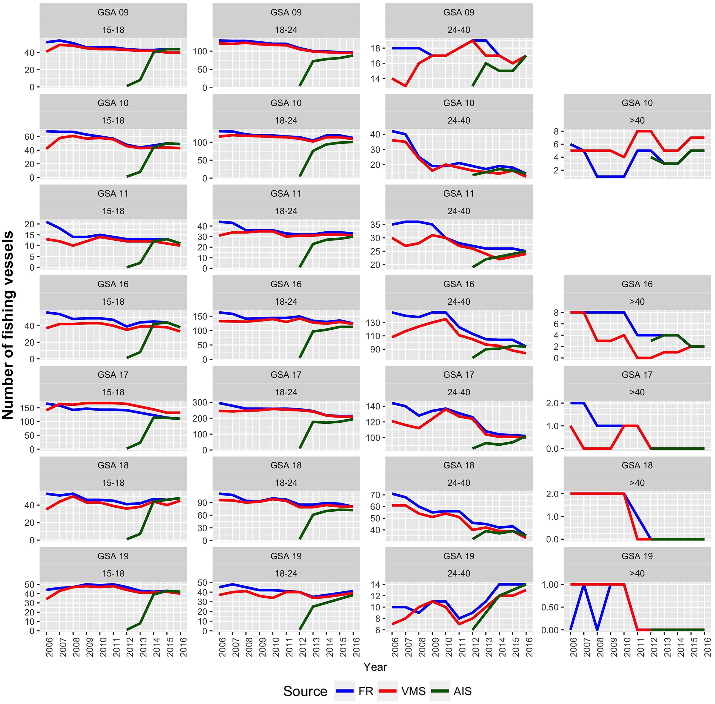
Figure 1. Coverage of VMS and AIS, by year/GSA and length segment, with respect to the official data downloaded from the Community Fishing Fleet Register (http://ec.europa.eu/fisheries/fleet/index.cfm).

Since the temporal coverage of fishing activity provided by the AIS are significantly lower that the correspondent value for the VMS (Russo et al., 2016b), a set of 195 fishing vessels equipped with both VMS and AIS were used to evaluate their agreement and representativeness in documenting fishing activity at a daily scale.

For each of these vessels and for each day of the year 2016, we classified VMS and AIS as “enabled” or “disabled” if at least one ping was present in the respective dataset. The aggregated results of this comparison are represented in Figure 2A.

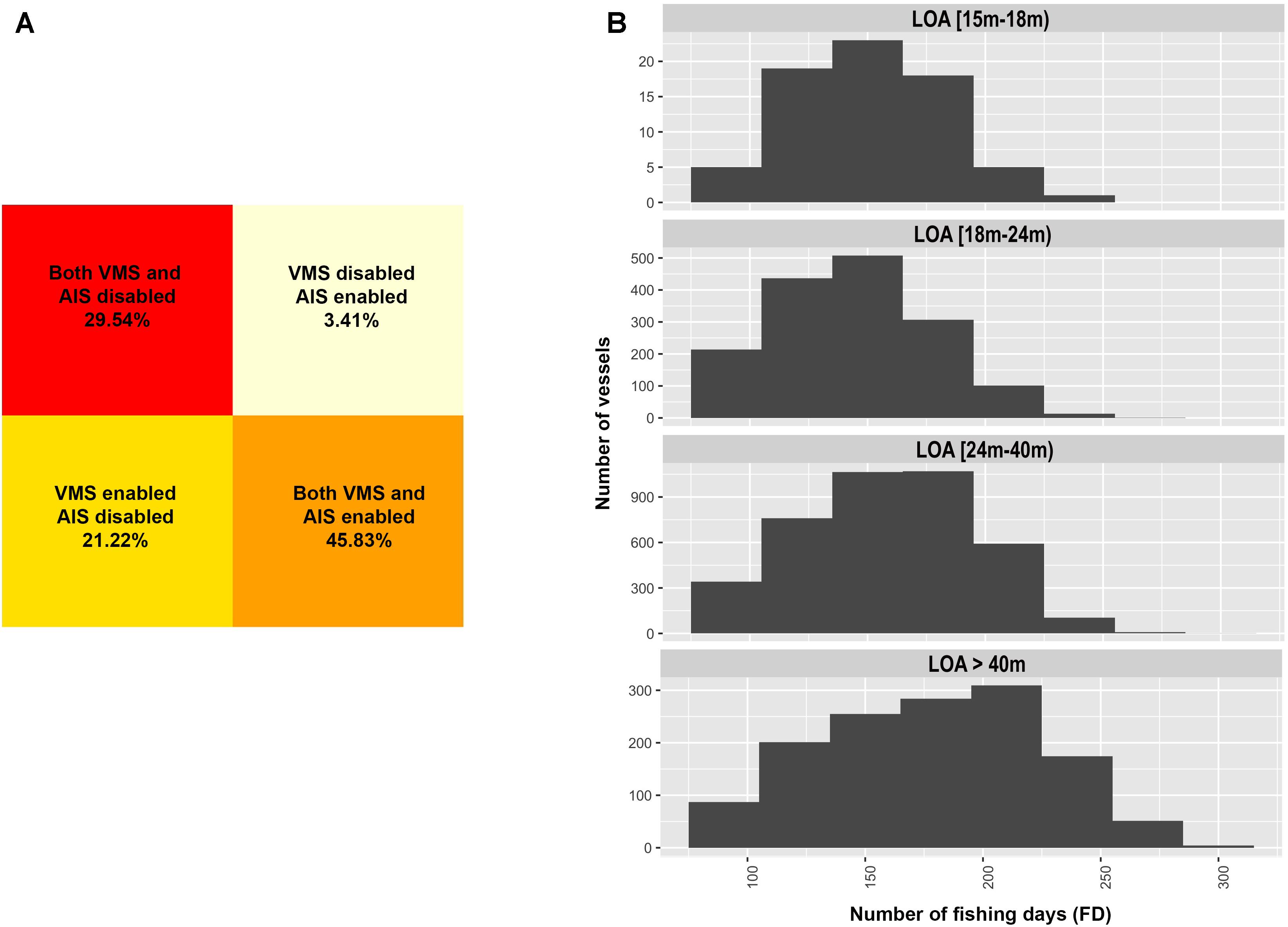
Figure 2. (A) Agreement between VMS and AIS in tracking the daily activity of 195 fishing vessels equipped with both systems, during the year 2016; (B) Histograms (by length classes) of the total number of fishing days by year for the OTB_over15 fleet equipped with VMS.

This comparison returned the evidence that, while in the 75.37% of cases the two tracking devices agree each other, there is a 21.22% of cases in which the VMS reports activity for the vessel whereas the AIS does not. Conversely, only in the 3.41% of cases the AIS reports activity for the vessel whereas the VMS does not. In other words, while the coverage of AIS data in terms of OTB_over15 fleet is now quite satisfactory, this device still does not guarantee an adequate assessment of vessels activity. Considering all these aspects (fleet coverage, assessment of fishing activity, temporal coverage for the inspected period), we limited the successive analyses to the period 2009–2016, using the VMS data as the source of information about Italian OTB_over15 fleet fishing activity. However, the analysis of fishing days by length class also indicated that the larger is the vessels, the higher is the number of fishing days (Figure 2B). Accordingly, the length class was considered in the successive assessment of fleet activity.

Within DCF, the fishing effort is quantified as Nominal Effort (NE), that is the cumulate sum of the Kw × Days at Sea of the fishing vessels belonging to the fleet. According to the INPDCF, the NE is assessed through questionnaires-based survey, performed on a subset of Italian harbors, of the fishing activity (i.e., the number of Days at Sea) of the different fleet segments. Here, an independent estimation of the fishing activity was obtained by computing, using VMS data, the mean annual number of fishing days (FD) of the OTB_over15 fleet by GSA and fleet segment.

In summary, raw VMS data for the years 2006–2016 were cleaned (by removing duplicates and erroneous pings), sorted by time and partitioned into fishing trips using the pings located near a harbor using the software platform VMSbase (Russo et al., 2011a,b, 2014a). After these steps, VMS pings were interpolated to increase the temporal and spatial representativeness of the activity and fishing set positions (i.e., trawling hauls) were identified using a combined deep/speed filter. This procedure returned, for each trawler, the pings classified as “fishing” for each calendar day of the period inspected. The total fishing days for each year/vessel was computed as the number of calendar days in which fishing pings were present.

The mean values of FD by length classes and GSA or combination of GSAs, estimated on the subset of vessels equipped with VMS, were expanded to the whole OTB_over15 fleet (as defined in the CFR) to estimate the total yearly NE by GSA and length according to the following equation:

where NE_y,g is the total Nominal Effort in year y and GSA g, nVess_l,y,g is the number of vessels in the official fleet of the GSA g during the year y, meanPW_l,y,g is the mean engine power of the vessels in the length class l of official fleet of the GSA g during the year y, and meanFD_l,y,g is the mean number of fishing days estimated from the VMS data for the same fleet.

These independent estimates of NE were compared to the official DCF ones and aggregated at the scale of GSA to investigate their relationship with landings and fishing mortality for some key stocks.

Furthermore, the NE was computed, for each year, with respect to the standard 3 × 3 km square grid used within the DCF-Module V (Ecological indicators of fishing pressure), according to the following equation:

where NE_y,c is the total Nominal Effort in year y and cell c, N is the total number of vessels operating in the cell c, PW_n is the engine power of the vessel n and FD_n,y is the number of fishing days estimated from the VMS data for the vessel n. FD_n,y was estimated using the procedure of the R package fecR (Scott et al., 2017). It is important to stress that this spatial estimation of the Nominal Effort was aimed only to describe the spatial distribution of fishing effort of the Italian OTB_over15 fleet and, in particular, to define the area of activity of the trawlers distributed in the Italian harbors. Hence, for this purpose, only the observed fishing activity (by VMS data) was considered. The mean NE value for each cell of this grid, computed across the years 2009–2016, is shown in Figure 3.

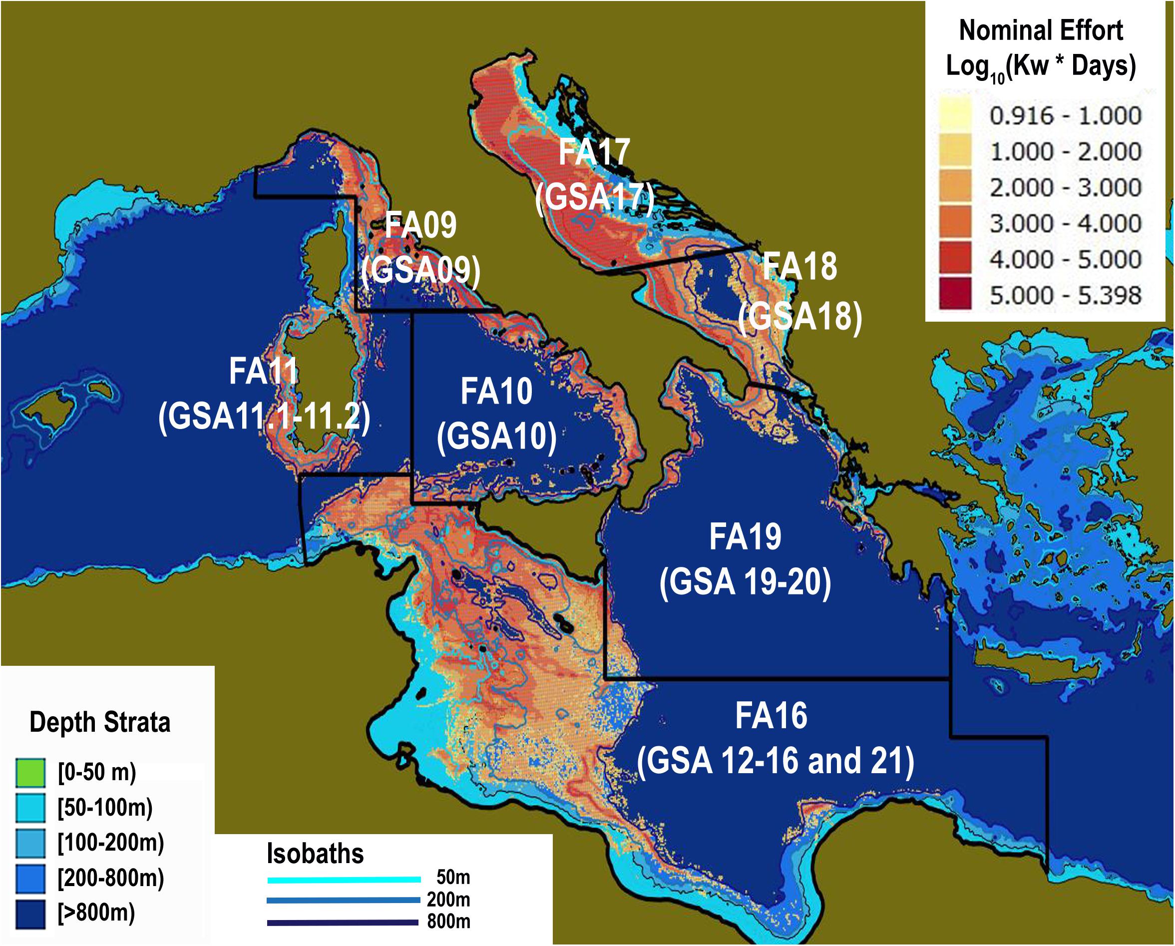
Figure 3. Mean annual distribution of the trawling nominal effort by the OTB₁₅ fleet during the period 2009–2016. The grid used to assess the Nominal Effort is the standard 3 × 3 km square used within the EU DCF. The logarithmic scale was used to better represent the pattern, while the main depth strata are reported.

According to the official harbor of registration of each vessel, we divided the Italian OTB_over15 fleet by GSA, and we assumed that the OTB_over15 fleet registered into each Italian GSA exploits a Fishing Area (FA) identified as the cells of the corresponding GSA (or set of GSAs, such as the case of the Strait of Sicily) with positive values of NE during the inspected period. For instance, in the case of the Strait of Sicily, we assumed that the FA16 area corresponds to the cells of the GSA12- 16 and 21 in which positive values of Nominal Effort were computed. A small group of vessels operating in the Levantine Sea has been excluded from the analyses. The main characteristics of the FAs are reported in Table 1. They represent, for each GSA-specific OTB_over15 fleet, the combined portion of shelf and slope exploited by trawl fishing and were used in the successive analysis to estimate both the values of Fisheries Yield and of Primary Production by GSA and year.

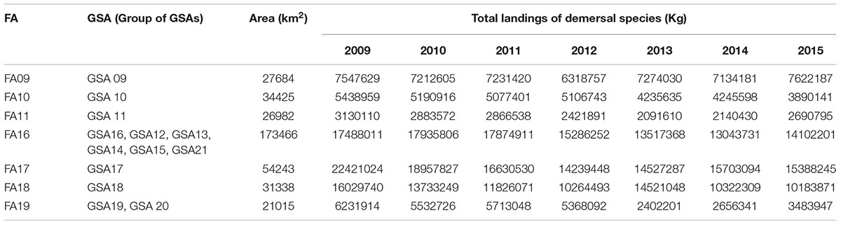
Table 1. Data for total landings of demersal species (source: Italian National Program of Data Collection in the Fisheries Sector) and estimated surface of the corresponding Fishing Area for each official GSA-specific fleets of Italian trawlers.

Primary Productivity and Production: Vertically Generalized Production Model (VGPM)

The primary productivity estimates returned by the Vertically Generalized Production Model (VGPM – Behrenfeld and Falkowski, 1997) available online at the Ocean Productivity Website³ were used to estimate the total Primary Production (PP) for each GSA or group of GSAs and year. The VGPM assumes that the Daily C fixed primary production (PP_eu, measured in mg C m^-2) integrated from the surface to the Euphotic depth (Z_eu) is a function of five parameters: (i) Maximum C fixation rate within a water column [P^B_opt, measured in mg C (mg CHL)^-1 h^-1]; (ii) sea surface Photosynthetically Active Radiance (PAR, measured in mol quanta m^-1); (iii) surface chlorophyll-a concentration Chlorophyll-a at P^B_opt (C measured in mg Chl m^-3); (iv) Euphotic depth (Z_eu, measured in m); and (v) Day length or photoperiod (D_irr, measured in hours).

The VGPM is widely used in the literature to estimate PP using environmental parameters retrieved from satellite data. The estimates of primary productivity provided as monthly XYZ files from MODIS R2014 Data were spatially attributed to the FA. Then, a mean value of productivity was computed for each FA/year and multiplied by the corresponding FA to obtain a value for each year and FA.

Landings of Demersal Species and Single Stocks Data

The total landings by year and GSA-specific fleet of trawlers for all the demersal stocks were obtained by the INPDCF, for the years 2009–2015. Italian landings data are collected through a statistical sampling scheme based on the distribution of the trawling fleet by GSA. Therefore, these landings are routinely assigned to the GSA of the harbor in which each vessel lands the catches, irrespectively of the original marine area of fishing activity. This fact implies that, in some cases (such as for the Sicilian trawling fleet landing in GSA 16), the area within which the fleets deploy their effort is larger than the GSA of official membership. According to the previous assumptions and steps of the analysis, we assumed that the official landings data for each GSA came from the respective FA (Table 1).

Species-specific landings data were further scrutinized to identify the main stocks in terms of contribution to the total landing by year and FA. Additionally, the estimated current Fishing mortality (F) and the related reference point (F_MSY) for the main (in terms of total annual landings) stocks of FA were collected from the literature (Cardinale et al., 2017), updated to the period 2009–2016 using both STECF⁴ and GFCM SAC reports⁵, and used to compute the rate F/F_MSY. This rate is a standard index to assess the overexploitation of a given stock. Given that not all stocks were evaluated by an analytical stock assessment, and the values of the ratio F/F_MSY are always not available for all the Italian GSAs, we restricted the following analyses to five stocks among the most important ones in terms of landings and for which a good coverage by year/FA was guaranteed. Namely: Aristeus antennatus (ARS hereafter) in FA 9, 10, 11, and 19; Parapaenaus longirostris (DPS hereafter) in FA 9, 10, 16, 18, and 19; Merluccius merluccius (HKE hereafter) in all FAs; Mullus barbatus (MUT) in all FAs except FA 11; and Nephrops norvegicus (NEP hereafter) in FA 9, 10, 16, 17, and 18.

Statistical Analyses of Trends: Generalized Additive Models

Generalized Additive Models (GAMs - Hastie and Tsibarani, 1990) were used to model the trends for and the relationships among:

• Total landings for demersal species (L_TOT) by FA;

• Landing per unit effort (LPUE) for the OTB_over15 fleet (as ratio between L_TOT and NE) by FA;

• The Overexploitation Ratio (F/F_MSY) by FA for the five stocks listed above.

GAMs are non-parametric regression techniques that allow for the modeling of relationships between variables without specifying any particular form for the underlying regression function. The use of smooth functions as regressors gives GAMs greater flexibility over parametric (including linear) types of models.

The predictors used for each independent variable are summarized in Table 2.

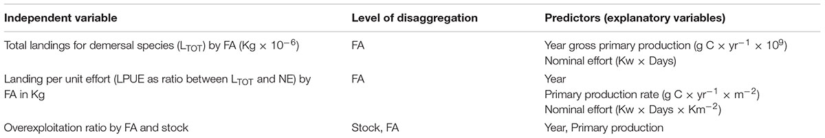
Table 2. List of predictors (regressors) used for the GAMs.

Given that multicollinearity among explanatory variables may increase the probability of Type I errors, predictors was tested using the Variance Inflation Factor (VIF) provided by the function vifcor of the R package “usdm” (Naimi, 2017).

This function vifcor iteratively finds pairs of variables which have the maximum linear correlation and, if this correlation is greater than a fixed threshold, excludes the one of them which has greater VIF. However, no predictors were excluded using this procedure, and then all the GAM regressions were performed using the full set of explanatory variables.

Starting from the full model (that included all explanatory variables), the most parsimonious model was selected on the basis of the lowest Akaike Information Criterion (AIC). Model goodness of fit was compared using the deviance and coefficient of determination (adjusted R²). All modeling was carried out using the “gam” library (Hastie, 2018), which implements cubic regression splines function to model the smoothness of predictors. Residuals for each model were graphically inspected to detect eventual departures from the model assumptions or other anomalies in the data (Cleveland, 1993). Final models were evaluated by comparing predictions and observations in a graphical way.

Data Sources and Model: Assumptions and Limitations

Two partially-overlapped temporal periods were examined in this study, given that not all the different data sources were available for the years 2009–2016. In particular:

• Effort data (VMS/AIS) were analyzed for the years 2006–2016, but the Nominal Effort was estimated only for the years 2009–2016, since the fleet coverage of VMS/AIS data for the years 2006–2008 was considered inadequate;

• Overexploitation rate and landings for the different stocks were analyzed for the years 2009–2015;

• The reconstruction of the Primary Production and the integrated modelling approach (i.e., GAM) was thus limited to the period 2009–2015.

It is worth noting that the modeling approach applied is characterized by some critical assumptions, which could be further addressed in future investigations. First of all, we analyzed the landings data for aggregated demersal resources without considering their internal structure in terms of proportion of the different species and related age classes. This implies that the trophic level of the demersal community exploited by the trawlers is assumed as virtually constant. Given that the trophic level is a key parameter influencing the cascade effect of the primary production on the trophic chain (Conti and Scardi, 2010; Conti et al., 2012; Fortibuoni et al., 2017), it is possible that important changes in the structure of catches and of the populations at sea are not captured by the GAMs.

Another potential limitation of this study is that the primary production estimated by remote sensing data could be biased near the coasts and do not provide any information about structure of the phytoplankton in terms of species and size classes. The first aspect is largely debated within the scientific community, but innovative and powerful approaches are continuously disseminated and could lead to more precise estimates in the future (Mattei et al., 2018). The latter aspect could have a relevant effect on the energetic transfer within the marine ecosystem.

An Ecosystem-based management should be “an interdisciplinary approach that balances ecological, social and governance principles at appropriate temporal and spatial scales in a distinct geographical area to achieve sustainable resource use […]” (Long et al., 2017). When applied to fisheries management, this means that the models used to provide advices and forecast the potential effects of management measures must move from the single-species approach used in stock assessment to more complex approaches in which species interactions, environmental drivers and human consequences are considered (Collie et al., 2014). While the transition from single-species toward ecosystem modeling is already advanced within the scientific community (Collie et al., 2014), we argue that for the EU management approach, from the legal (Commission Regulations and Directives) and technical point of views, the roadmap is still in late. One of the obstacle to this process could be represented by the observations that while the increasing of model complexity often improves model fit, also the outputs uncertainty increases (Collie et al., 2014). Another issue is related to the fact that complex models (e.g., ECOSIM or ATLANTIS) are data demanding and the datasets needed to support them are often available only at a small scale or for short temporal series. Multispecies and ecosystem models are valuable tools for providing insights into key system dynamics but they are not useful as tools for holistic management since they do not provide robust tactical advices (Benson and Stephenson, 2018). A realistic target could be the progressive orientation toward models of intermediate complexity such as ISIS_FISH (Mahévas and Pelletier, 2004; Pelletier et al., 2009), SMART (Russo et al., 2014b), DISPLACE (Bastardie et al., 2014), MICE (Punt et al., 2014) explicitly devised to work with data collected within the DCF (Lehuta et al., 2016). These models, which could be scored as “intermediate” in terms of complexity, often correspond to the “sweet spot” at which uncertainty in outputs (including policy indicators) is at a minimum (Collie et al., 2014). The present study would contribute to this debate by demonstrating that the combined usage of state-of-the-art approaches for monitoring of fishing activities and satellite-based information about primary production could effectively improve our ability to analyze the response of the productivity and exploitation state of fished stock under the pressure of natural and anthropic drivers.

Results

Fishing Activity and Fishing Effort

The temporal trends of mean fishing activity by FA and trawler length class (Figure 4) suggest that, in most cases, an increase of the mean number of fishing days by year occurred during the last years. This increase is statistically significant (if fitted using a simple linear model with intercept) in nine over 21 cases: the two largest length classes in the North Tyrrhenian Sea and in the Strait of Sicily, the smallest length class in the Ionian Sea, the largest vessels in Sardinia, and all the length classes in the North Adriatic Sea. In general, the number of additional fishing days by year is near to four, but it reaches 9–10 for the largest vessels in the North Tyrrhenian Sea, in Sardinia, and in the Strait of Sicily. Although not significant, apparent increasing trends could be observed in the other cases, with the exception of Sardinia. The reconstructed trends of NE, obtained by aggregating the fleet segments by FA, is illustrated in Figure 5 and compared with the independent DCF estimates. In five over seven FAs the trends are very similar, whereas they consistently differ for FA17 and 18. In these two FAs, both located in the Adriatic Sea, the VMS-based effort is larger than the DCF one. For the FA17 (North Adriatic), the VMS-based NE is almost always (i.e., with the exception of the year 2011) 1.4 times the DCF one. For FA18 (South Adriatic), the two series progressively diverge with time, the VMS-based being in mean 1.6 times the DCF one. However, in all the FA, it is possible to notice an increasing trend of NE in the last 2–3 years of the series (2015–2016). This is particularly apparent for the FAs 16 and 18, where the trends were previously decreasing.

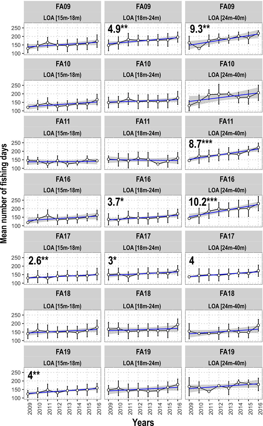
Figure 4. Trends of the mean l number of fishing days by year, FA and length class, as obtained by the analysis of VMS data. The significant coefficients, as number of additional fishing days by year, are reported and marked by ^∗p < 0.05 or ^∗∗p < 0.005.

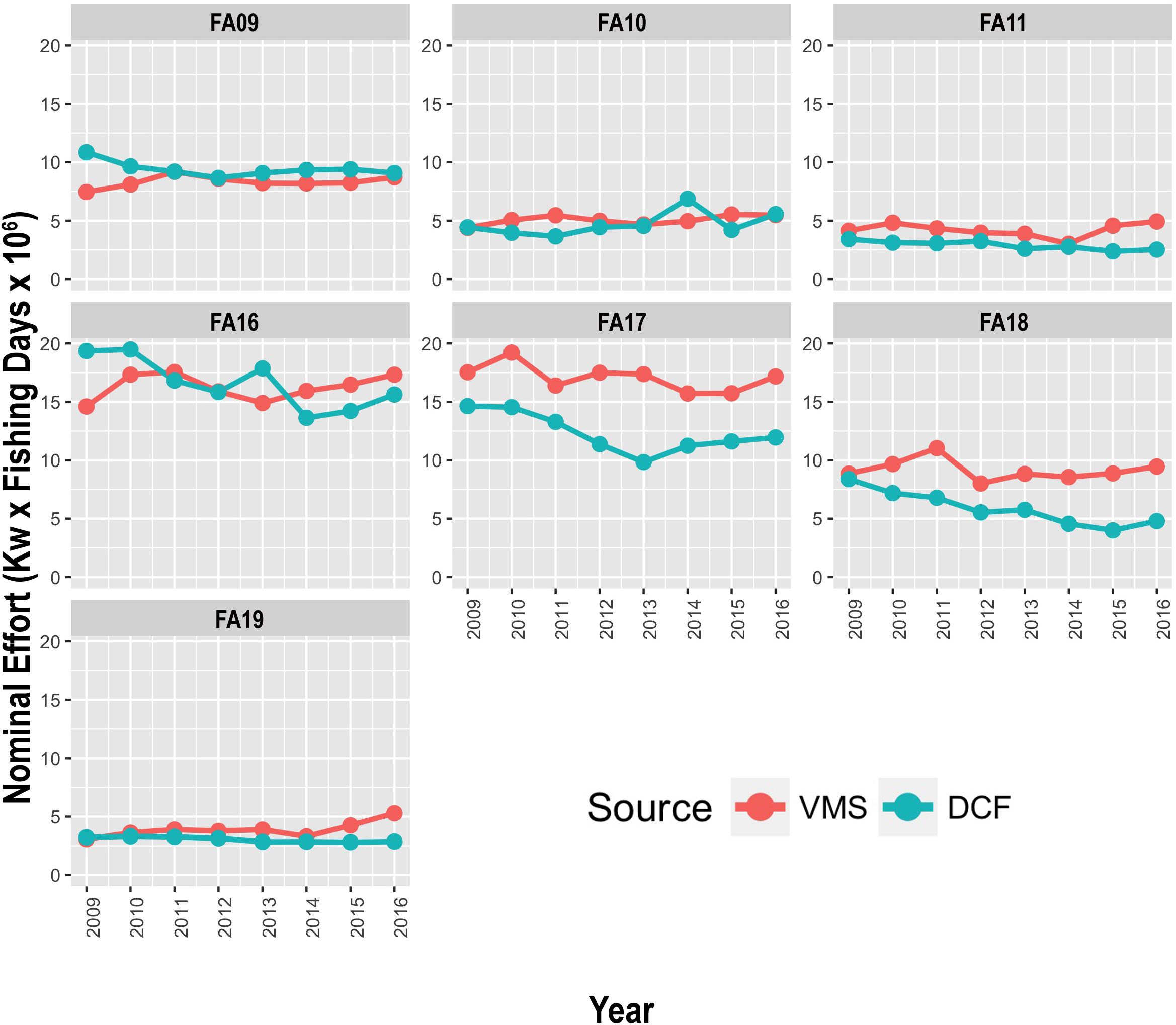
Figure 5. Comparison of DCF trends for the Nominal Effort (NE in Kw × Days of fishing × 106) with the one obtained using the VMS data.

Primary Production

The trends for PP rate by FA returned by the VGPM approach are represented in Figure 6. In most cases, a minimum could be identified for the year 2012, whereas two relative maxima occurred for the year 2010 and 2013, the latter being often the absolute maximum of the series. The rest of the trends is fluctuating between these extremes, with larger fluctuations detectable in FA17 and a more stable pattern for FA16. In general, the highest values correspond to FA17, while the lowest occur in FA16 and FA19.

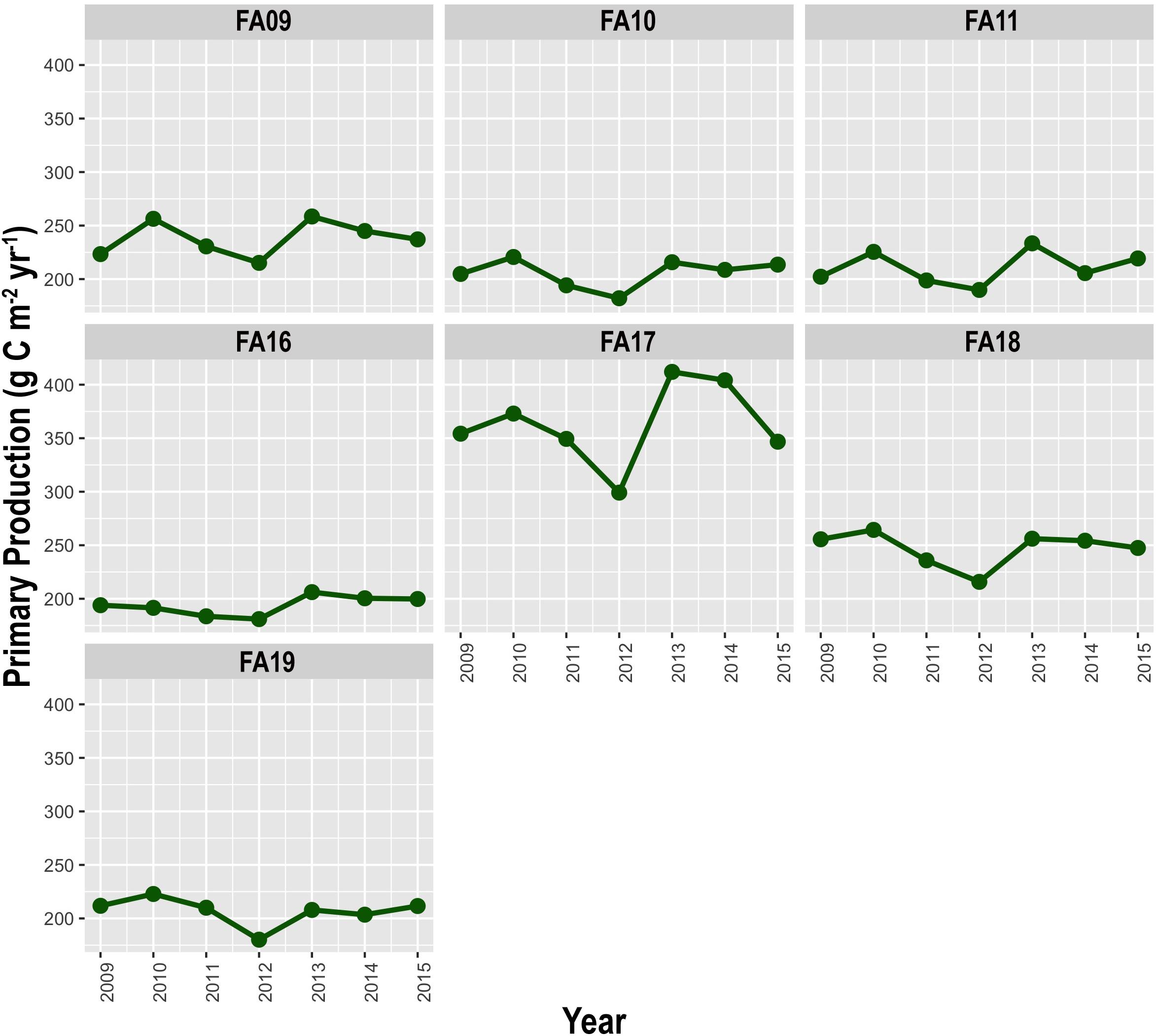
Figure 6. Trends for Primary Production rate (PP in g C m^-2 yr^-1) by FA, as reconstructed using the VGPM approach (data available online at the Ocean Productivity Website http://orca.science.oregonstate.edu/2160.by.4320.monthly.hdf.vgpm.m.chl.m.sst.php).

Relationship Between Fishing Effort, Primary Productivity and Fisheries Productivity

When the mean annual spatial indexes of NE, PP and fisheries yield for the demersal species (i.e., the landings) are compared between FAs (Figure 7), it is possible to recognize three statistically significant monotonic correlations (Spearman’s rho values in Figure 7). The largest variability characterizes the index of fisheries yield, which depends both by PP (Figure 7A) and even more by NE (Figure 7B). In all the cases, the FA16 (Strait of Sicily) is associated with the lowest values of all the variables, thus representing the bottom-left extreme of the pattern: low primary productivity, low fishing effort and low fisheries productivity. The opposite situation is represented by the Adriatic Sea (FA17 and FA18). The variability around the mean values (standard error bars of Figure 7) indicates that the fisheries yield is the more unstable variable, whereas PP and NE slightly changed during the years inspected. Globally considered, Fisheries Yield, Primary Production and Nominal Effort allow distinguishing between two blocks of FAs (Figure 7D): the first one (comprising the FAs 9, 17, and 18) characterized by values of FY larger than 2.5 Kg ha^-1 yr^-1, and the second one (FAs 10, 11, 16, and 19) characterized by values of FY below 2.5 Kg ha^-1 yr^-1.

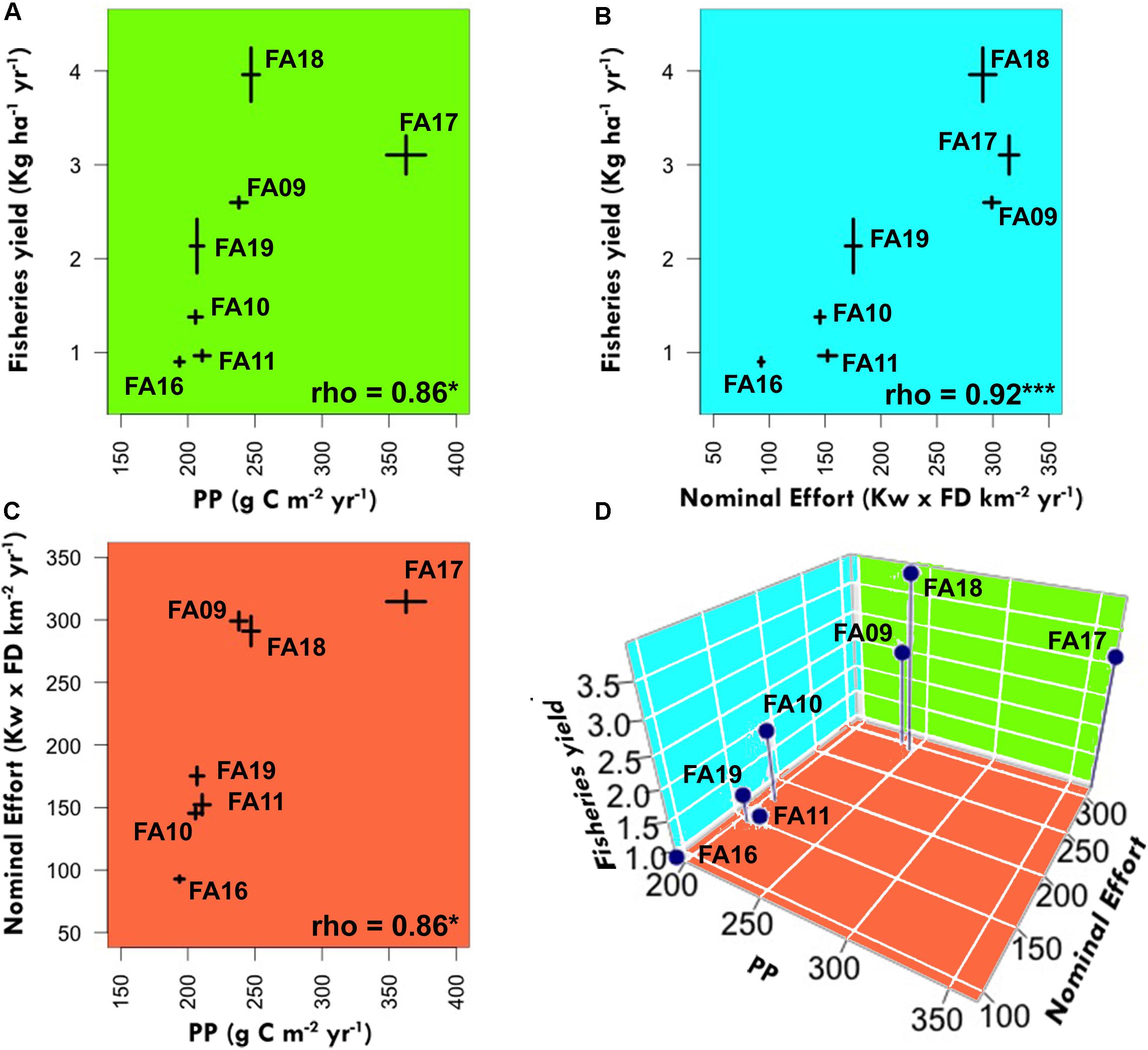
Figure 7. Relationships between: (A) primary productivity (PP) and fisheries yield for demersal species; (B) nominal effort and fisheries yield; (C) primary productivity (PP) and nominal effort; (D) all the three factors together. Variability in PP (horizontal bars) and fisheries yield (vertical bars) are shown, for each FA in the parts (A–C) of the plot, as standard error around the mean values.

Generalized Additive Models

Fisheries Yield

The analysis of the temporal trends of Landings (Figure 8 and Table 3) returned, in most of the cases, decreasing patterns which are well captured by GAMs. More in detail, a falling phase is always detectable in the period 2009–2012. During these 4 years, landings lost around 20% of their values in all the FAs. The second phase (years 2013–2015) is characterized by a progressive recovery in some FAs (namely FA 9, 11, and 19), a substantial stability (FA 16, 17, and 18), or a further decrease (FA10). The GAMs captured well all the decreasing trends and the stable phases, whereas they diverge from the DCF trends when the second phase is characterized by a recovery.

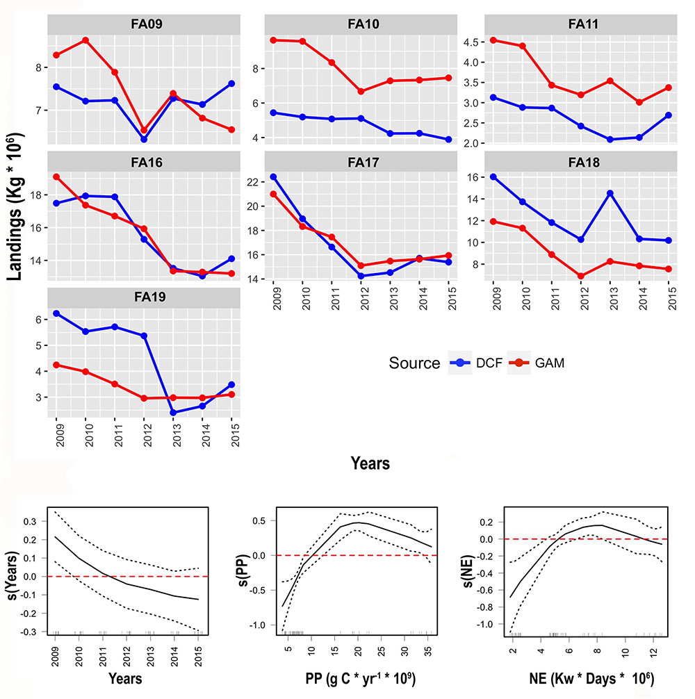
Figure 8. (A) Comparisons between actual trends (source: DCF, blue lines and dots) and GAM-based models of Fisheries Yield, during the period 2009–2015. The effects of the different predictors (if significant), independent of the other predictors, are represented as response variable shape. The degree of smoothing is indicated in the y-axis label. (B) Confidence intervals (95%) around the response curve are represented by dashed lines.

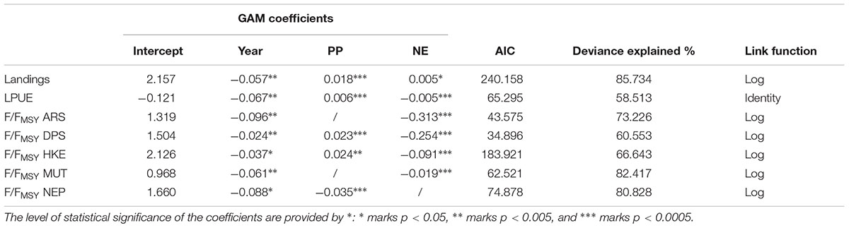
Table 3. Summary of GAM results for the F/F_MSY of the five selected species.

ANOVA for Non-parametric Effects of the predictors included in the GAM model of FY indicates that all the predictors have a significant effect on the dependent variable (Figure 8B). A negative and slightly curvilinear relationship is found for the predictor year, with the highest values of landings associated with the first years of the time series. The shape of the PP effect recalls an asymptotic function. Landings increase monotonically with increasing PP until it reaches a value of around 15+ 10⁹ gC yr^-1 but, above this value, landings remain stable or slightly decrease. The shape of the smoother for NE is similar: landings growth until NE reaches a value of ∼ 6^∗10⁶ Kw^∗Days and. The percentage of deviance captured by the GAM is highly satisfactory (above 85% of the total).

Landing per Unit Effort

The analysis of the temporal trends of LPUE (Figure 9 and Table 3) returned a series of outputs very similar to the ones described for Landings. Also in this case, the trends are characterized by a substantial decrease along the temporal period considered and all the predictors are statistically significant.

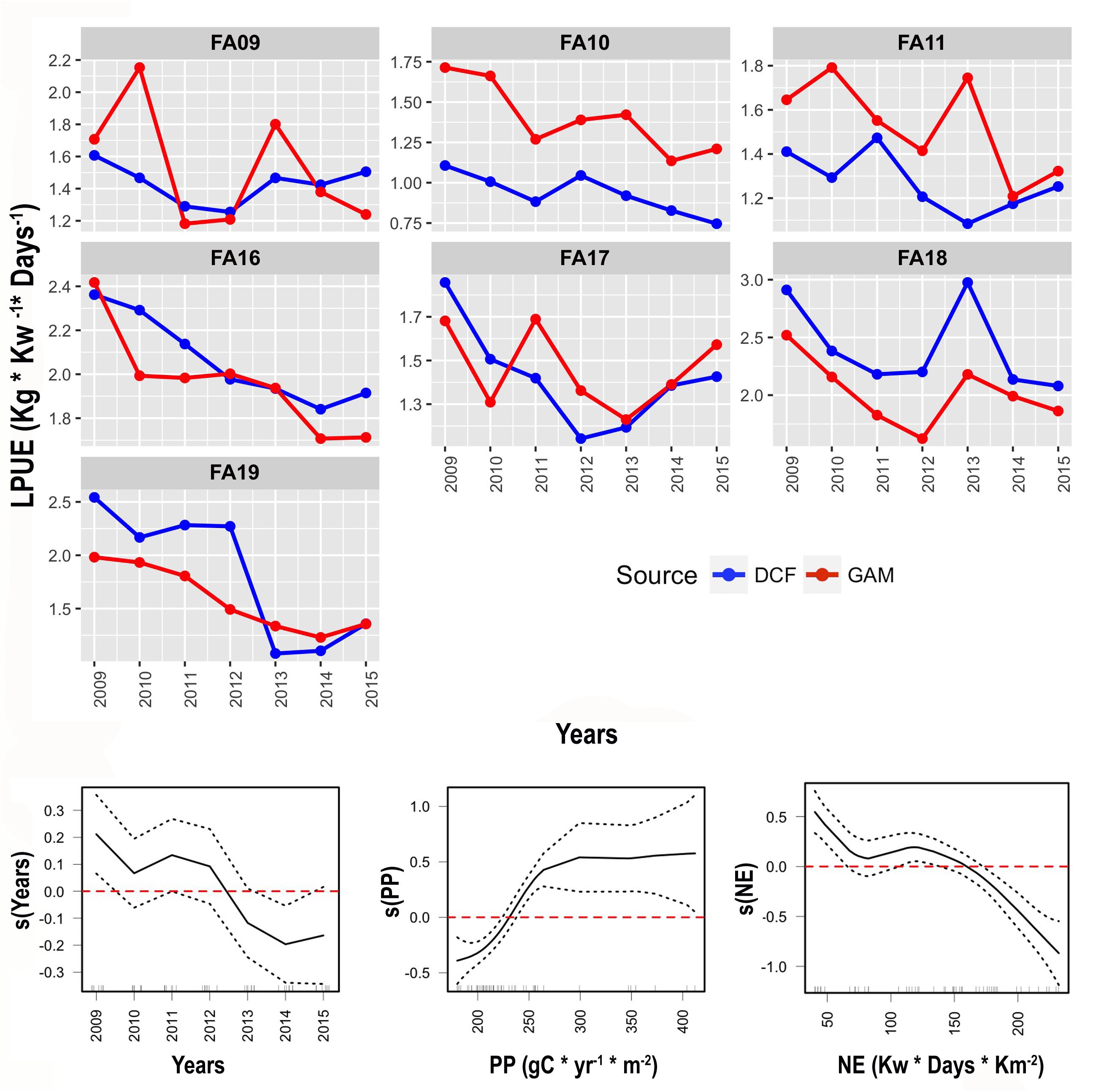
Figure 9. (A) Comparisons between actual trends (source: DCF, blue lines and dots) and GAM-based models of LPUE, during the period 2009–2015. (B) The effects of the different predictors (if significant), independent of the other predictors, are represented as response variable shape. The degree of smoothing is indicated in the y-axis label. Confidence intervals (95%) around the response curve are represented by dashed lines.

Also in this case, two distinct phases seem occurring. However, the declining phase (years 2009–2012) is followed by an increasing phase in FA17 and, to a lesser extent, in FA 9, 11, and 19. The other FAs are characterized by further decrease (FA16) or a substantial stability (FA18). The smoothers of the different predictors are partially coherent with the GAM applied on Landings with the exception of NE, which is negatively related to the LPUE when the NE is low. The shape of the NE effect shows also an abrupt decrease above 150 Kw Days Km^-2. The predictor Year has a fluctuating effect, but the global pattern is inversely linked to LPUE. LPUE shows an asymptotic relationship with PP, with the plateau reached for values of PP above 300 gC yr^-1 m^-2. The percentage of deviance captured by the GAM is satisfactory (above 58% of the total) but suggests that some additional predictors should be integrated into the model.

Relative Overexploitation Rate (F/F_MSY)

The GAM trends for the overexploitation rate (F/FMSY – Figure 10 and Table 3) well captured the observed ones in most cases: ARS in FA11 and 19; DPS in FA16 and 19; HKE in FA11, 17, and 19; MUT in FA17 and 19; NEP in FA16 and FA18. In the other cases, some discrepancies between GAM and DCF trends are detectable. However, the worst results in terms of GAM fitting occurred for the two of the FAs (9 and 10) belonging to the Tyrrhenian Sea. The percentage of deviance explained by the specific GAMs ranges from 60% (DPS) to 82% (MUT). The best models for DPS and HKE contain all the predictors, whereas PP were not present in the models for ARS and MUT and NE was not present in the best model for NEP. The trends are globally decreasing during the inspected period, with some exceptions in the last 2–3 years.

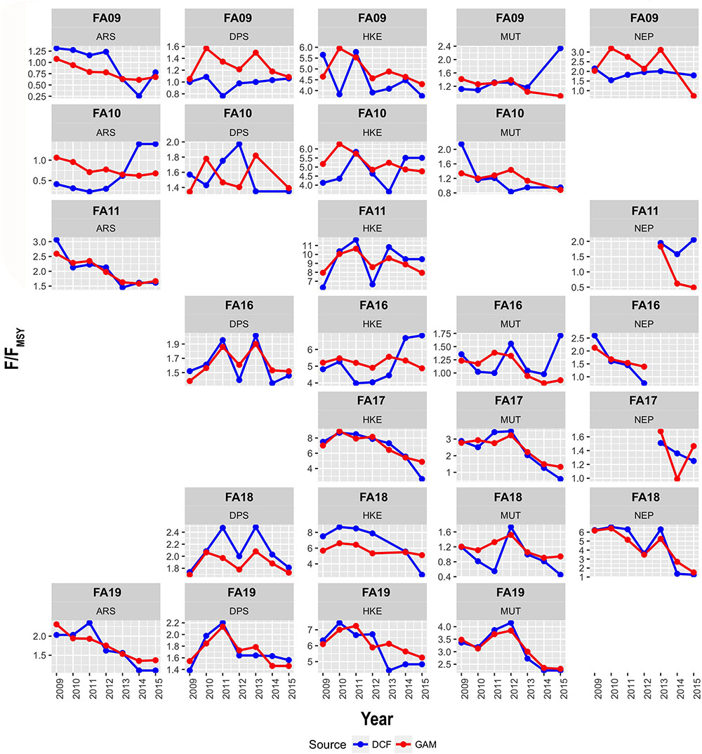
Figure 10. Comparisons between actual trends (source: DCF, blue lines and dots) and GAM-based models (red lines and dots) of the ratio F/FMSY, during the period 2009-2015.

The shapes of the effects of the different predictors Year and PP on F/FMSY (Figure 11) closely recall the ones described for the LPUE, whereas the effect of NE on F/FMSY is somewhat counterintuitive. In fact, F/FMSY for DPS, HKE and MUT reaches the minimum values for intermediate levels of effort.

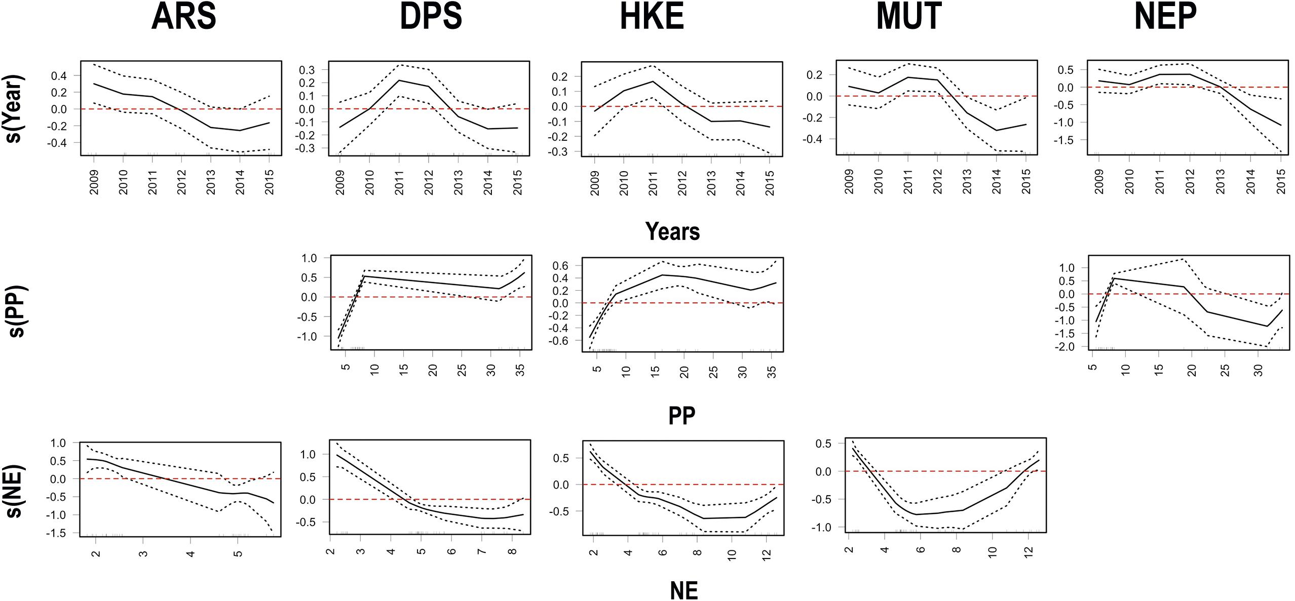
Figure 11. Effects of the different predictors (if significant), independent of the other predictors, are represented as response variable shape for each species. The degree of smoothing is indicated in the y-axis label. Confidence intervals (95%) around the response curve are represented by dashed lines.

Discussion

Following a logical sequence, the results of this paper suggest that:

(1) The real area of activity of the trawlers nominally belonging to the seven Italian FAs is, in some cases, much wider than the membership FA (Figure 3). In particular, Italian trawlers landing into the south of the Sicily exploit a huge area, extended from the coasts of the Tunisia to the Libya, covering almost all the fishing grounds of the Strait of Sicily;

(2) The trends of the fishing activity as number of fishing days (Figure 4) obtained using VMS data always show an increasing tendency which is, in some cases, statistically significant. This means that, while the fishing capacity was substantially reduced, the remaining fleet partially counterbalanced this reduction by increasing its activity. As a result, the Nominal Effort obtained using VMS and AIS shows, in most FAs, a substantial stability over the inspected period (Figure 5). This stability is the result of two opposite tendencies: a first decrease in the period 2009–2013, reasonably determined by the reduction of the fleet size, followed by a recover in the period 2014–2016 at least partially determined by the increase of fishing activity per vessel. It is important to notice that the trends of Nominal Effort are largely coherent with the official DCF ones, with the exception of the Adriatic FAs where a reduction is reported by the DCF effort.

(3) The spatial index for Primary Productivity estimated for the real areas of activity of the FA-specific trawling fleet shows fluctuating trends (Figure 6) with relevant differences between years. These fluctuations are coherent between the FAs and evidence that the years 2010 and 2013 were characterized by two relative maxima, whereas the year 2012 was the absolute minimum during the inspected period;

(4) The comparison between index of fisheries yield (limited to the landings of demersal species), both PP and NE per unit of surface (Figure 7) by FA or group of FAs evidences a monotonic and statistically significant effect of these factors on the amount of demersal resources landed in the different Italian Seas. Moreover, it allows recognizing that the Adriatic Sea is the most productive area, which is a somewhat expected result, but also that the Strait of Sicily is the less productive area since its fleets operates on a wide portion of the central Mediterranean (Figure 3). The wide area over which the fishing effort of the Sicilian trawlers (FA16) is distributed is also characterized by low level of primary productivity;

(5) The modeling exercise of fisheries landings and fisheries productivities (LPUE) for demersal species (Figures 8, 9) evidences that the three predictors used (year, trawling effort and primary production) allow capturing a large portion of the variability and return, in most of the cases, well suited models. In almost all of the cases the predictor year is characterized by an inverse relationship with the response variable. Accordingly, both landings and LPUE decrease with time in all the FAs;

(6) The relationship between gross primary production and landings of demersal species has an asymptotic shape (Figure 8). However, almost all the observations are located in the steeped part of the curve, with the exception of the data for the FA17 (Figure 12). This means that, in 6 over 7 FAs, the changes of the primary production are likely to determine important consequences for the amount of landings;

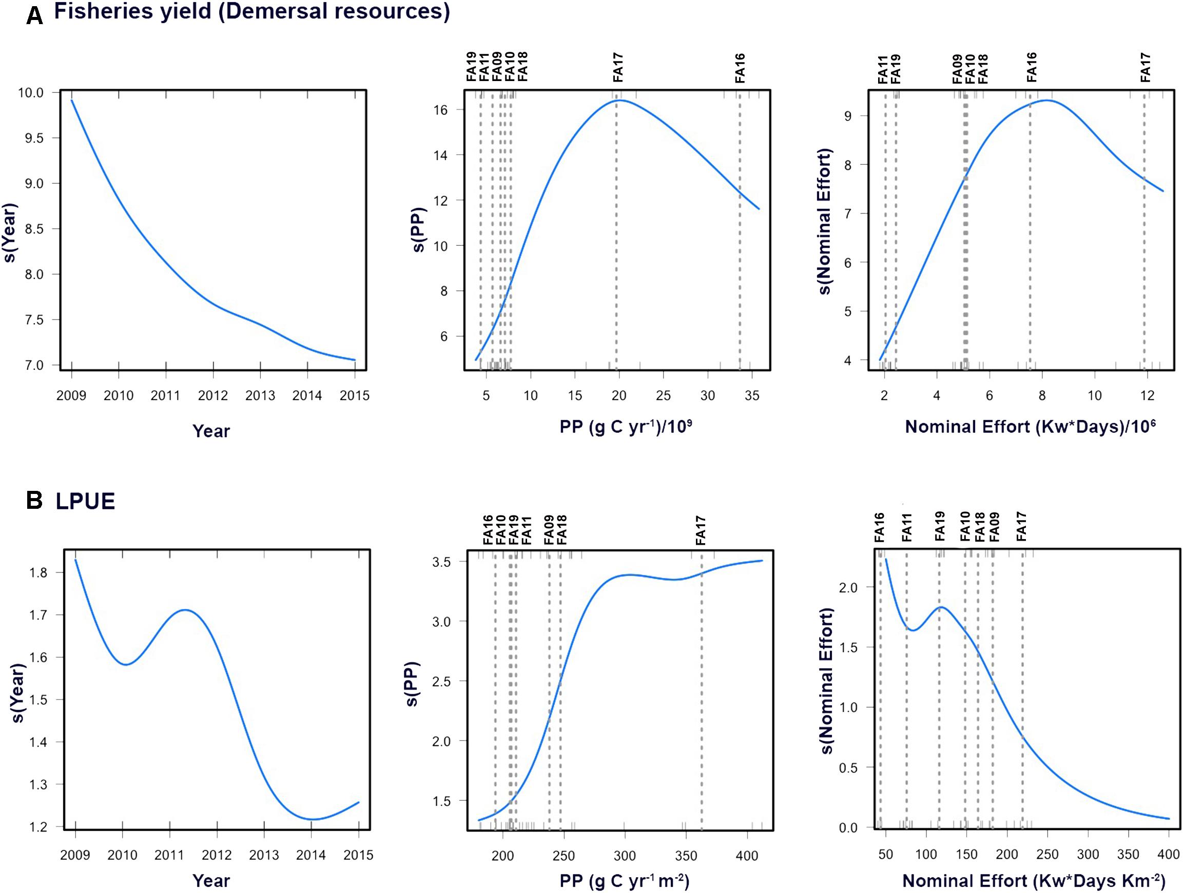
Figure 12. Summary of the effect of year, PP and NE on (A) Fisheries yield and (B) LPUE across the seven FA examined.

(7) The fishing effort, quantified as Nominal Effort, is associated to an asymptotic effect on landings and a substantially inverse effect on LPUE. Both these results are coherent with the literature on relationships between yield and fishing effort (Hilborn and Walters, 1987) and could be interpreted by considering the different realities represented by the Italian FAs: the Adriatic Sea is the portion of Mediterranean Sea with the highest concentration of trawlers. This fact, together with the presence of a large shelf area, allows reaching the highest values of absolute NE and NE per unit of surface. As evidenced in Figure 12, the NE in FA17 is located in the plateau region of the effect on landings, meaning that a reduction of the trawling effort is likely to determine a positive effect on both landings and LPUE. In the other FAs, an increase of the fishing effort should determine a potential increase of landings accompanied by a reduction of the LPUE;

(8) The GAMs well captured the trends of the ratio F/F_MSY and report that, in most of the cases, this ratio is moving toward more acceptable values. However, the last 2 years (2015–2016) of the period analyzed often show a reverse of this tendency. This happens always for the ARS and for DPS and MUT in FA16 and FA19. This increase of the overexploitation ratio (ratio F/F_MSY) in the most recent years could be due was to the recent increase of the fishing effort, at least in some FAs (Figure 5);

(9) The responses of the stock to the predictors are more variable (Figure 11). The ratio F/F_MSY is associated, for 4 over 5 stocks, to two phases of decrease in the extremes of the temporal period separated by a phase of increase in the years 2010–2012. DPS, HKE and NEP are significantly influenced by the primary productivity by an asymptotic-like relationship, and all the stocks with the exception of NEP show an inverse relationship between the ratio F/F_MSY and the NE, suggesting that the exploitation of these stocks could be more efficient with lower levels of trawling effort.

From a methodological point of view, this paper attempts to introduce some potentially important innovation. For the first time VMS data were explicitly used to obtain an independent estimate of the fishing effort. Although the obtained estimates substantially agree with the official ones, they seem more sensitive in capturing some actual trends, such as the rising of the fishing activity (and then of the fishing effort) occurred in the last 2 years (2015–2016 – Figure 5).

The core of this paper is actually devoted to the application of a relatively simple modeling approach in which two drivers (fishing effort and primary productivity) are used as proxies of the contrasting forces working, in combination with the time, on demersal resources and influencing the corresponding landings. Recently presented an analysis of all available stock assessments and effort data for the most important commercial species and fleets in the Mediterranean Sea since 2003 was presented (Cardinale et al., 2017). Using a GAM-based modeling approach, these authors showed that: (1) Fishing mortality (F) is larger or much larger than F_MSY for all species and it has remained stable during the last decade for almost all species; (2) there is no apparent relationship between nominal effort and fishing mortality for all species. According to these authors the predictor time is devised to capture the “inertial” component present in the trend of each response variable, that is the cumulative effects of the exploitation pattern exerted in the past years on the demersal communities of the FAs. However, while Cardinale et al. (2017) used the FA as a factor in their GAM approach (with has no intercept), here we fitted a model in which the differences between FAs are related only to the intercept of the relationship, whereas the effects of the predictors are the same for all the FAs. In this way, the models presented in this study are more general and allow comparing the status of the different FAs (Figure 12). Given that the usage of the FA as a factor technically means that the number of fitted GAM models corresponds to the number of FAs, some inconsistencies between our results and those of Cardinale et al. (2017) (e.g., about the effect of fishing effort) could be explained by the lower statistical power of the GAM models with lower number of observations. Moreover, the work of Cardinale et al. (2017) could be framed within the classical approaches used by EU management bodies since the status of the stocks is analyzed using only time and fishing effort as predictors.

The current status of fisheries and ecosystems in the Mediterranean Sea is a worrisome picture in which the overfishing acts together with the ongoing climate forcing and additional phenomena such as the rapid expansion of non- indigenous species (Colloca et al., 2017). This study would like to represent a step beyond in this direction, since it incorporates the role of the primary production, which is a function of both environmental changes (e.g., sea water temperature, hydrodynamic regime) and factors heavily influenced by human activities (e.g., nutrients inlets). The key role of PP is confirmed by some results: the landings for the year 2012, which corresponds to the minimum value of PP in the inspected period, are the lowest values in 4 of the 7 FAs. This correspondence is particularly clear for the FA17 and FA18, that is the Adriatic Sea.

Conclusion

In terms of assessment and of management advices, the results of this study could be summarized as follows:

(1) The general depletion of demersal resources is confirmed along all the temporal series analyzed (Figure 12A – Year) and, while a partial recovery of LPUE (Figure 12B – Year) was observed in the year 2011–2012 (probably linked to the reduction of fishing capacity), a progressive decrease of landing and of LPUE was observed during the last years (2013–2015). This inversion was probably determined by the increase of the fishing activity which eroded the positive effect of the reduction of the fishing capacity producing a new increase of the fishing effort;

(2) In all the seven FAs investigated, the LPUE are inversely related to the level of NE observed (Figure 12B – NE). This means that a reduction of the effort is expected to determine a higher economic efficiency of the trawlers;

(3) Apart from the case of North Adriatic Sea (FA17), in the other FAs the landings of demersal species are constrained by their level of primary productivity as (Figure 12B – PP);

(4) Although the Strait of Sicily and adjacent seas are characterized by a low productivity (Figure 12B – PP), the wide area exploited by trawlers supports an important gross primary production (Figure 12A – PP). However, for the same reason, the Italian trawlers landing into the Sicilian harbors cannot efficiently exploit the fishing grounds very far from the Sicilian coasts. This allows understanding why the FA16 scores higher in Figure 12A – PP and lower in Figure 12B – PP,

(5) The current Mediterranean National Management Plans⁶ are still based on one stock/species and one GSA, not fully explaining the real situation and trends. The General Fisheries Commission for the Mediterranean⁷, on the other hand, is implementing sub-regional and regional plans for shared species covering different GSAs. The results presented in this paper clearly support the GFCM approach, also offering an alternative to move toward more appropriate temporal and spatial scale for management.

Data Availability

The datasets for this study will not be made publicly available because some of the original raw data (i.e. VMS) are protected by confidentiality. All the metadata are available under request.

Author Contributions

TR, SC, and MS conceived the ideas and designed the methodology. TR, PC, LD, MS, LL, GG, FF, and PD collected the data. TR, PC, LD, PDA, GG, SF, and AP analyzed the data. TR wrote the manuscript. All authors contributed critically to the drafts and gave final approval for publication.

Funding

This work has been supported by the Italian Ministry of Agricultural, Alimentary and Forestry Politics with the Research Project “Basi scientifiche e strumenti a supporto dei Piani di Gestione della pesca nell’ambito della Politica Comune della Pesca e delle politiche ambientali ed economiche.”

Conflict of Interest Statement

PC was employed by Maja Società Cooperativa a.r.l., while LL was employed by Società Cooperativa MABLY.

The remaining authors declare that the research was conducted in the absence of any commercial or financial relationships that could be construed as a potential conflict of interest.

Acknowledgments

We acknowledge Massimiliano Cardinale (Marine Research Institute, Swedish University of Agricultural Sciences) and Giuseppe Scarcella (Institute of Marine Sciences of the Italian National Research Council) for the fertile discussions about the modeling approach and for sharing some input data.

Footnotes

1. ^https://ec.europa.eu/fisheries/documentation/studies/stockmed_en
2. ^http://www.astrapaging.com/
3. ^https://modis.gsfc.nasa.gov/sci_team/pubs/abstract_new.php
4. ^https://stecf.jrc.ec.europa.eu/reports/medbs
5. ^http://www.fao.org/gfcm/reports/statutory-meetings/en/
6. ^https://ec.europa.eu/fisheries/cfp/fishing_rules/multi_annual_plans_en
7. ^https://ec.europa.eu/fisheries/press/42nd-annual-session-general-fisheries-commission-mediterranean-milestones-mediterranean-and_en

References

Amoroso, R. O., Pitcher, C. R., Rijnsdorp, A. D., McConnaughey, R. A., Parma, A. M., Suuronen, P., et al. (2018). Bottom trawl-fishing footprints on the world’s continental shelves. Proc. Natl. Acad. Sci. U.S.A. 115, E10275–E10282. doi: 10.1073/pnas.1802379115
Bastardie, F., Rasmus Nielsen, J., and Miethe, T. (2014). DISPLACE: a dynamic, individual-based model for spatial fishing planning and effort displacement — integrating underlying fish population models. Can. J. Fish. Aquat. Sci. 71, 366–386. doi: 10.1139/cjfas-2013-0126
Behrenfeld, M. J., and Falkowski, P. G. (1997). Photosynthetic rates derived from satellite-based chlorophyll concentration. Limnol. Oceanogr. 42, 1–20. doi: 10.4319/lo.1997.42.1.0001
Benson, A. J., and Stephenson, R. L. (2018). Options for integrating ecological, economic, and social objectives in evaluation and management of fisheries. Fish Fish. 19, 40–56. doi: 10.1111/faf.12235
Blanchard, J. L., Jennings, S., Holmes, R., Harle, J., Merino, G., Allen, J. I., et al. (2012). Potential consequences of climate change for primary production and fish production in large marine ecosystems. Philos. Trans. R. Soc. B Biol. Sci. 367, 2979–2989. doi: 10.1098/rstb.2012.0231
Cardinale, M., Osio, G. C., and Scarcella, G. (2017). Mediterranean Sea: a failure of the european fisheries management system. Front. Mar. Sci. 4:72. doi: 10.3389/fmars.2017.00072
Carpi, P., Scarcella, G., and Cardinale, M. (2017). The saga of the management of fisheries in the adriatic sea: history, flaws, difficulties, and successes toward the application of the common fisheries policy in the mediterranean. Front. Mar. Sci. 4:423. doi: 10.3389/fmars.2017.00423
Chassot, E., Mélin, F., Le Pape, O., and Gascuel, D. (2007). Bottom-up control regulates fisheries production at the scale of eco-regions in European seas. Mar. Ecol. Prog. Ser. 343, 45–55. doi: 10.3354/meps06919
Collie, J. S., Botsford, L. W., Hastings, A., Kaplan, I. C., Largier, J. L., Livingston, P. A., et al. (2014). Ecosystem models for fisheries management: finding the sweet spot. Fish Fish. 17, 101–125. doi: 10.1111/faf.12093
Colloca, F., Scarcella, G., and Libralato, S. (2017). Recent trends and impacts of fisheries exploitation on mediterranean stocks and ecosystems. Front. Mar. Sci. 4:244. doi: 10.3389/fmars.2017.00244
Conti, L., Grenouillet, G., Lek, S., and Scardi, M. (2012). Long-term changes and recurrent patterns in fisheries landings from large marine ecosystems (1950–2004) author links open overlay panel. Fish. Res. 11, 1–12. doi: 10.1016/j.fishres.2011.12.002
Conti, L., and Scardi, M. (2010). Fisheries yield and primary productivity in large marine ecosystems. Mar. Ecol. Prog. Ser. 410, 233–244. doi: 10.3354/meps08630
Cowan, J. Jr. (1996). Size-dependent vulnerability of marine fish larvae to predation: an individual-based numerical experiment. ICES J. Mar. Sci. 53, 23–37. doi: 10.1006/jmsc.1996.0003
Cury, P., Mullon, C., Garcia, S., and Shannon, L. (2005). Viability theory for an ecosystem approach to fisheries. ICES J. Mar. Sci. 62, 577–584. doi: 10.1016/j.icesjms.2004.10.007
Fortibuoni, T., Giovanardi, O., Pranovi, F., Raicevich, S., Solidoro, C., and Libralato, S. (2017). Analysis of long-term changes in a mediterranean marine ecosystem based on fishery landings. Front. Mar. Sci. 4:33. doi: 10.3389/fmars.2017.00033
Friedrichs, M. A. M., Carr, M. E., Barber, R. T., Scardi, M., Antoine, D., Armstrong, R. A., et al. (2009). Assessing the uncertainties of model estimates of primary productivity in the tropical Pacific Ocean. J. Mar. Syst. 76, 113–133. doi: 10.1016/j.jmarsys.2008.05.010
Hastie, T. (2018). Package “gam”: Generalized Additive Models. Available at: https://cran.r-project.org/web/packages/gam/index.html
Hilborn, R., and Walters, C. J. (1987). A general model for simulation of stock and fleet dynamics in spatially heterogeneous fisheries. Can. J. Fish. Aquat. Sci. 44, 1366–1369. doi: 10.1139/f87-163
Hunter, M. D., and Price, P. W. (1992). Playing chutes and ladders: heterogeneity and the relative roles of bottom-up and top- down forces in natural communities. Ecology 73, 724–732.
Lehuta, S., Girardin, R., Mahévas, S., Travers-Trolet, M., and Vermard, Y. (2016). Reconciling complex system models and fisheries advice: practical examples and leads. Aquat. Living Resour. 29:208. doi: 10.1051/alr/2016022
Long, R. D., Charles, A., and Stephenson, R. L. (2017). Key principles of ecosystem-based management: the fishermen’s perspective. Fish Fish. 18, 244–253. doi: 10.1111/faf.12175
Macias, D., Garcia-Gorriz, E., and Stips, A. (2018). Major fertilization sources and mechanisms for mediterranean sea coastal ecosystems. Limnol. Oceanogr. 63, 897–914. doi: 10.1002/lno.10677
Mahévas, S., and Pelletier, D. (2004). ISIS-Fish, a generic and spatially explicit simulation tool for evaluating the impact of management measures on fisheries dynamics. Ecol. Model. 171, 65–84. doi: 10.1016/j.ecolmodel.2003.04.001
Mattei, F., Franceschini, S., and Scardi, M. (2018). A depth-resolved artificial neural network model of marine phytoplankton primary production. Ecol. Model. 382, 51–62. doi: 10.1016/j.ecolmodel.2018.05.003
McCluskey, S. M., and Lewison, R. L. (2008). Quantifying fishing effort: a synthesis of current methods and their applications: quantifying fishing effort: methods review. Fish Fish. 9, 188–200. doi: 10.1111/j.1467-2979.2008.00283.x
Naimi, B. (2017). Package ‘usdm’: Uncertainty Analysis for Species Distribution Models. Available at: https://cran.r-project.org/web/packages/usdm/index.html
Pelletier, D., Mahevas, S., Drouineau, H., Vermard, Y., Thebaud, O., Guyader, O., et al. (2009). Evaluation of the bioeconomic sustainability of multi-species multi-fleet fisheries under a wide range of policy options using ISIS-Fish. Ecol. Model. 220, 1013–1033. doi: 10.1016/j.ecolmodel.2009.01.007
Planque, B., Fromentin, J.-M., Cury, P., Drinkwater, K. F., Jennings, S., Perry, R. I., et al. (2010). How does fishing alter marine populations and ecosystems sensitivity to climate? J. Mar. Syst. 79, 403–417. doi: 10.1016/j.jmarsys.2008.12.018
Punt, A. E., Hurtado-Ferro, F., and Whitten, A. R. (2014). Model selection for selectivity in fisheries stock assessments. Fish. Res. 158, 124–134. doi: 10.1016/j.fishres.2013.06.003
Reid, D. G., Graham, N., Rihan, D. J., Kelly, E., Gatt, I. R., Griffin, F., et al. (2011). Do big boats tow big nets? ICES J. Mar. Sci. 68, 1663–1669. doi: 10.1093/icesjms/fsr130
Russo, T., Carpentieri, P., Fiorentino, F., Arneri, E., Scardi, M., Cioffi, A., et al. (2016a). Modeling landings profiles of fishing vessels: an application of self-organizing maps to VMS and logbook data. Fish. Res. 181, 34–47. doi: 10.1016/j.fishres.2016.04.005
Russo, T., D’Andrea, L., Parisi, A., Martinelli, M., Belardinelli, A., Boccoli, F., et al. (2016b). Assessing the fishing footprint using data integrated from different tracking devices: issues and opportunities. Ecol. Indic. 69, 818–827. doi: 10.1016/j.ecolind.2016.04.043
Russo, T., D’Andrea, L., Parisi, A., and Cataudella, S. (2014a). VMSbase: an R-package for VMS and logbook data management and analysis in fisheries ecology. PLoS One 9:e100195. doi: 10.1371/journal.pone.0100195
Russo, T., Parisi, A., Garofalo, G., Gristina, M., Cataudella, S., and Fiorentino, F. (2014b). SMART: a spatially explicit bio-economic model for assessing and managing demersal fisheries, with an application to italian trawlers in the strait of sicily. PLoS One 9:e86222. doi: 10.1371/journal.pone.0086222
Russo, T., Parisi, A., and Cataudella, S. (2011a). New insights in interpolating fishing tracks from VMS data for different métiers. Fish. Res. 108, 184–194. doi: 10.1016/j.fishres.2010.12.020
Russo, T., Parisi, A., Prorgi, M., Boccoli, F., Cignini, I., Tordoni, M., et al. (2011b). When behaviour reveals activity: assigning fishing effort to métiers based on VMS data using artificial neural networks. Fish. Res. 111, 53–64. doi: 10.1016/j.fishres.2011.06.011
Scott, F., Prista, N., and Reilly, T. (2017). FecR: A Package For Calculating Fishing Effort. Available at: https://rdrr.io/cran/fecR/f/inst/doc/calculating_fishing_effort.pdf
Sinclair, M., and Valdimarsson, G. (2003). Responsible Fisheries in the Marine Ecosystem. Rome: Organisation of the United Nations. doi: 10.1079/9780851996332.0000
Smedbol, R., and Stephenson, R. (2001). The importance of managing within-species diversity in cod and herring fisheries of the north-western Atlantic. J. Fish Biol. 59, 109–128. doi: 10.1111/j.1095-8649.2001.tb01382.x
STECF (2014). 41th Plenary Meeting Report of the Scientific, Technical and Economic Committee for Fisheries (PLEN-12-03) Plenary Meeting 5-9 November 2012, Brussels. Luxembourg: Publications Office.
Keywords: fisheries, spatial management, effort, VMS, primary production, mortality, sustainability, stocks
Citation: Russo T, Carpentieri P, D’Andrea L, De Angelis P, Fiorentino F, Franceschini S, Garofalo G, Labanchi L, Parisi A, Scardi M and Cataudella S (2019) Trends in Effort and Yield of Trawl Fisheries: A Case Study From the Mediterranean Sea. Front. Mar. Sci. 6:153. doi: 10.3389/fmars.2019.00153
Received: 22 December 2018; Accepted: 11 March 2019;
Published: 02 April 2019.
Edited by:
Mercedes González-Wangüemert, Centro de Ciências do Mar (CCMAR), PortugalReviewed by:
M. Cristina Mangano, Bangor University, United KingdomFabio Pranovi, Università Ca’ Foscari, Italy
Copyright © 2019 Russo, Carpentieri, D’Andrea, De Angelis, Fiorentino, Franceschini, Garofalo, Labanchi, Parisi, Scardi and Cataudella. This is an open-access article distributed under the terms of the Creative Commons Attribution License (CC BY). The use, distribution or reproduction in other forums is permitted, provided the original author(s) and the copyright owner(s) are credited and that the original publication in this journal is cited, in accordance with accepted academic practice. No use, distribution or reproduction is permitted which does not comply with these terms.
*Correspondence: Tommaso Russo, Tommaso.Russo@Uniroma2.it