Predicting Fishing Footprint of Trawlers From Environmental and Fleet Data: An Application of Artificial Neural Networks

Introduction

The modern fishery sciences are largely based on spatial data that show the activity of fishing vessels (McCluskey and Lewison, 2008; Amoroso et al., 2018). The appraisal of tracking devices, such as the Vessel Monitoring System (VMS) and the Automatic Identification System (AIS), have opened a new era for the investigation of fishing behavior and have supported the development of a new generation of bio-economic and ecological models of the interactions between fleets and resources (Bastardie et al., 2014; Russo et al., 2014b; Girardin et al., 2017). Until now, hundreds of scientific research articles have been published regarding the spatial and temporal dynamics of fishing vessels that are equipped with one of (or both) these tracking devices, but of course, the frontier of this revolution is represented by the portion of the fleets covered by the VMS and/or AIS. The issue of “hidden” (without VMS or AIS) vessels is common in many jurisdictions worldwide, while VMS/AIS usage is still undeveloped in some marine regions (see http://www.fao.org/fishery/topic/18072/en for details by country and by regional fisheries management organization). In the European Union (EU), both the VMS and AIS are compulsory only for some fleet segments, depending upon vessel size (i.e., the length-over-all – LOA). The VMS became compulsory for EU vessels longer than 15 m as of 2005, and for EU vessels longer than 12 m as of January 2012. The AIS is compulsory for all vessels longer than 15 m (from June 2013). Thus, given that EU fleets are largely composed of vessels below 12 m in LOA, and although both the VMS and AIS have progressively expanded their fleet coverage during the last decade (Russo et al., 2016b), some of the EU fleets are not covered by (at least) one of these tracking devices. The relevance of this partial coverage varies according to the structure of the fleets by country. With respect to the EU members bordering the Mediterranean Sea, Figure 1 shows the number of trawlers (fishing vessels performing bottom otter trawling that have the most impact on fisheries worldwide) with and without the VMS, by country and by length class. According to the European Data Collection Framework¹ (DCF), fishing vessels are grouped and monitored in the following length classes² : [6–12 m), [12–15 m), [15–24 m), and [24–40 m).

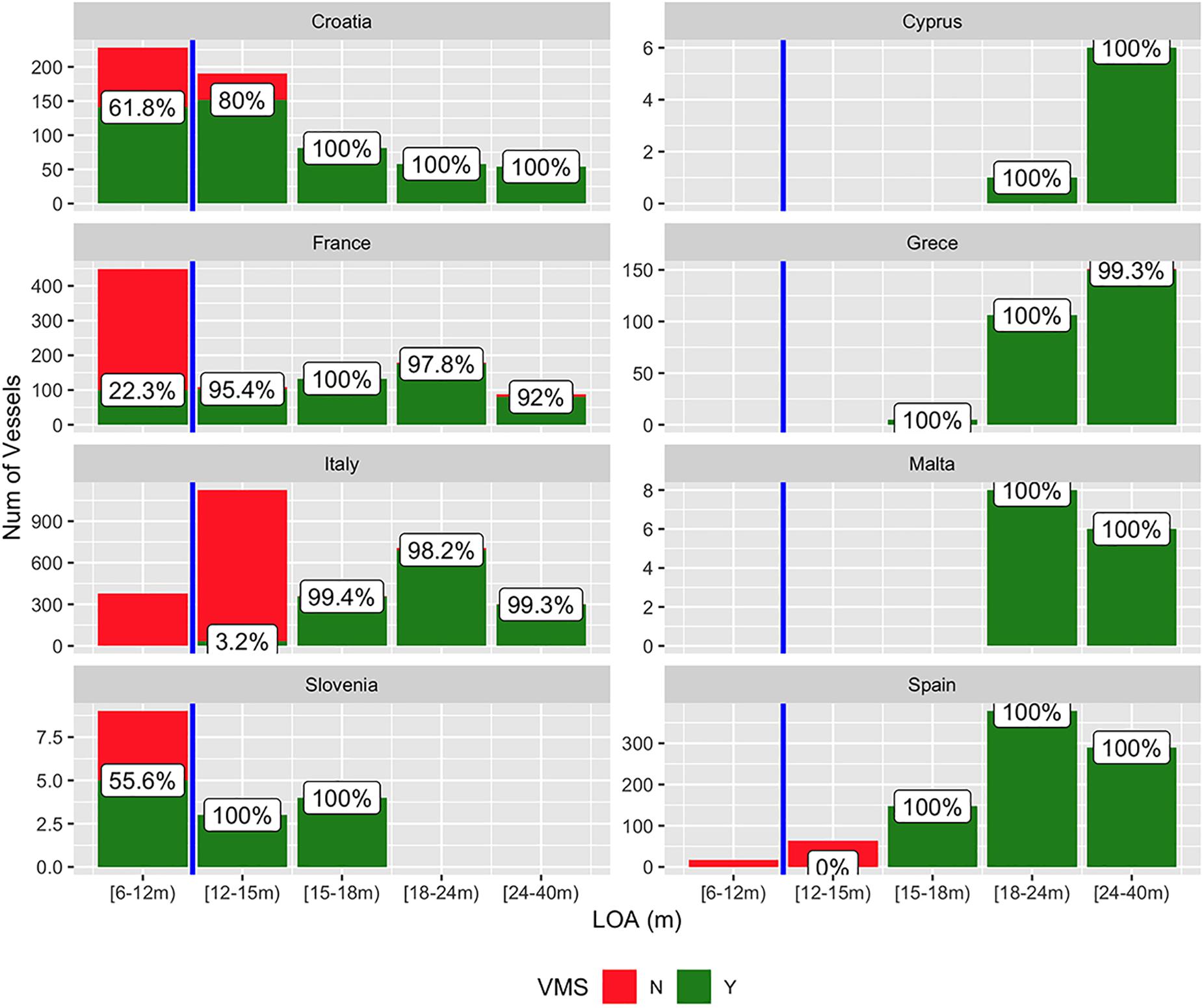
Figure 1. Frequencies of the number of trawlers by country and length class equipped with the VMS (green) and without VMS (red). The percentage values represent, for each length class, the coverage of the VMS. The vertical blue line represents the legal threshold for mandatory usage of the VMS in the EU countries, although the European Council Regulation (EC) No 1224/2009 allows the member states to exempt fishing vessels in the length class [12–15 m) if they: (a) operate exclusively within the territorial seas of the flag member state; and (b) never spend more than 24 h at sea from the time of departure to the return to port). Source: official EU Community Fleet Register (http://ec.europa.eu/fisheries/fleet/index.cfm).

Noticeably, the vessels with LOAs over 15 m are almost completely covered for all countries. In contrast, the coverage of the VMS for the length class [12–15 m) of the Italian, Spanish and Croatian fleets, three of the largest EU fleets operating in the Mediterranean Sea, is far from being complete: 80% of 190 trawlers for Croatia, 3.2% of the 1,125 trawlers for Italy, and none of the 63 trawlers for Spain. As a consequence, the footprints (“an area subject to human activity,” in this case trawl fishing – ASOC, 2011) of these trawlers cannot be directly quantified. The lack of a VMS onboard trawlers longer than 12 m is justified by European Council (EC) Regulation No 1224/2009, that allows member states to exempt fishing vessels with LOAs between 12 and 15 m if they: (a) operate exclusively within the territorial seas of the flag member state; and (b) never spend more than 24 h at sea from the time of departure to the return to port.

According to the Community Fishing Fleet Register³ (CFR), the subset of Italian trawlers that falls into this category and takes advantage of this exemption is mainly composed (53%) of vessels operating in the Adriatic Sea, the portion of the Mediterranean Sea that corresponds to the Geographic Sub Areas (GSA) 17 and 18 (see Figure 2A) as defined by the General Fisheries Commission for the Mediterranean. In fact, the large shelf of this semi-enclosed basin effectively supports a fleet largely composed of small trawlers, in contrast with other Mediterranean areas (e.g., the Strait of Sicily) in which trawlers are generally larger and operate farther from the harbors. Hence, the available estimates of the fishing footprints of trawlers in the Adriatic Sea are biased due to the lack of data related to the relevant fleet portions. Moreover, some of the VMS-based ecological indicators of fishing pressure used within DCF, as well as spatial analyses carried out within the new Fisheries Dependent Information⁴, do not consider these portions of the EU fleets and their fishing activities. Logbooks also represent a source of spatial data for fishing activity, but they are often characterized by different issues, including lack of accuracy and reliability of declared catches and the positions of fishing activities (Sampson, 2011; Russo et al., 2016b). In addition, the information logbooks convey is often aggregated at a daily scale.

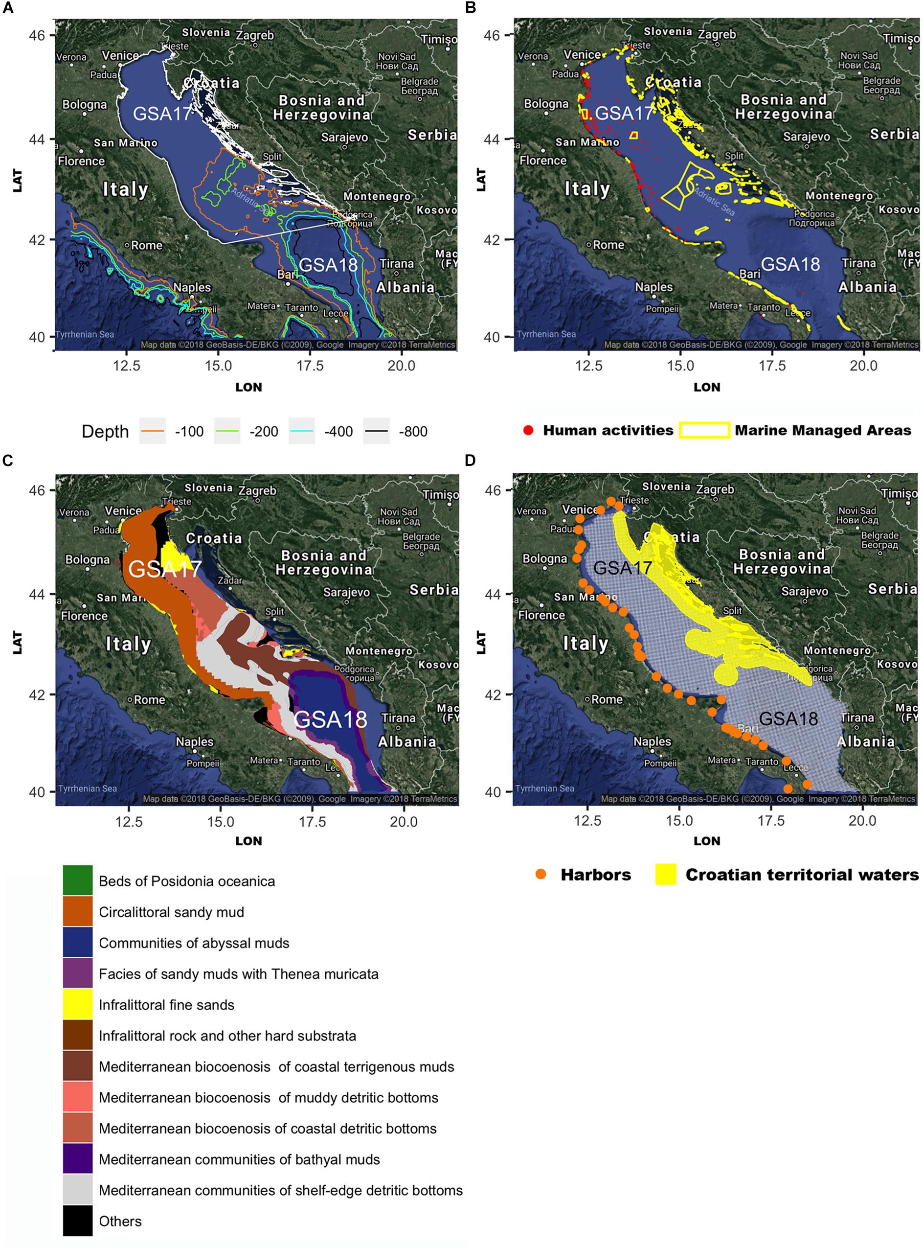
Figure 2. (A) Study area: the Adriatic Sea with the two FAO Geographical Sub Areas (GSAs) (white lines) and the main isobaths are shown; (B) human activities (in red) and marine managed areas (in yellow); (C) main bottom substrates obtained from the European Marine Observation Data Network (EMODnet) Seabed Habitats project (http://www.emodnet-seabedhabitats.eu/); and (D) the 3 × 3 km square grid (in gray) used within the DCF for the computations of the fishing pressure indicators; the Croatian territorial waters are excluded from the analysis. The figures were created using the R package ggmap (Kahle and Wickham, 2013) importing images from Google maps.

Currently, few quantitative approaches have been proposed to estimate the fishing footprints of vessels not equipped with remote tracking devices. Among these approaches, the application of multi-criteria decision analysis proposed by Kavadas et al. (2015) to estimate the potential fishing footprints of small scale fisheries represents one of the most promising approaches. Other approaches are based on: (1) the combined analysis of the number of boats and the local coastal human populations (Johnson et al., 2017); (2) the use of fishermen’s knowledge through geographical information systems (Léopold et al., 2014); (3) the cross-analysis of logbook data and vessel characteristics (Natale et al., 2015); and (4) the combination of participatory mapping with socioeconomic evaluations (Thiault et al., 2017).

However, these approaches are designed for passive fishing gear (trammel nets, gill nets, bottom or surface longlines, boat seiners and traps) and are completely independent from VMS or AIS data. The latter point is an advantage but is also a limitation, since (1) data from tracking devices provide a source of information for the relationships between vessel characteristics (LOAs, engine power, harbors of departure/landing) and spatial allocations of fishing efforts, and (2) their availability for subsets of the fleets could be used as a basis for inferring the behavior of the whole fleet. Here, we present and apply a method that combines static information of sea characteristics (e.g., depths and distances from the coast) and fleet structure/distribution by harbors (i.e., spatial allocations of fishing capacity) to predict the spatial distributions of fishing efforts at a yearly scale. The method learns from available georeferenced data for vessels with the VMS and allows extrapolation to the whole official fleet. The aim of the model is therefore to provide estimates of fishing footprints for entire fleets, even if only subsets of them are directly monitored by VMS or AIS. Here, the method is applied to the fleet of Italian trawlers that operate in the Adriatic Sea, and its estimates are evaluated through comparisons with independent logbook datasets.

The method is based on artificial neural networks (ANN), a group of modeling techniques that imitate the functioning of the human brain to analyze large and complex datasets characterized by non-linear relationships among variables, internal redundancy and noise (Lek and Guégan, 1999). We designed a cascaded multilayer perceptron network (CMPN hereafter – Watts and Worner, 2008) that is a sequence of two multilayer perceptron networks (MPN) in which the output from one MPN becomes the input to another MPN (Franceschini et al., 2018). MPN represents the simplest and most widely used ANN architecture (Lek and Guégan, 1999; Scardi, 2001; Haykin and Haykin, 2009; Quetglas et al., 2011). The applications of MPN in the framework of fisheries science include, among others, the modeling of time series (Schulz and Matthies, 2014), the forecasting of resource abundances (Yáñez et al., 2010), the identification of fishing set positions from VMS data (Joo et al., 2011), coastal engineering (Deo, 2010), the identification of fishing gear (Russo et al., 2011b) and the modeling of landing profiles (Russo et al., 2016a).

Materials and Methods

Study Area and Input Variables for the MPNs

The study area consists of the two neighboring areas, namely, GSA17 (Northern Adriatic Sea) and GSA18 (Southern Adriatic Sea), covering a total of approximately 121,668 km². The Northern Adriatic area is characterized by depths shallower than 100 m, except for the complex of the Pomo Pit, where depths achieve a maximum of over 200 m (Figure 2A). Several anthropic activities other than fisheries (e.g., aquaculture, and hydrocarbon extraction platforms) are present along the Italian coast (Figure 2B), while marine protected areas (MPA) are mainly represented by a large polygon around the Pomo Pit complex and by several smaller areas along the coasts (Figure 2B). The seabed mainly consists of the continental shelf, with circalittoral sandy muds and communities of shelf-edge detritic bottoms (Figure 2C). The following areas were excluded from the analysis: (1) the Croatian territorial waters (Figure 2D), within which Italian trawlers do not operate; and (2) the portions of the shelf with depths <50 m and distances <3 nautical miles within which trawling activities are forbidden. The rest of the Adriatic Sea was divided in 16,072 cells, each with a size of 3 × 3 km. This grid is the same as that used within the DCF for computation of the ecological indicators of fishing pressures 5, 6, and 7 (Russo et al., 2011a; Lambert et al., 2012). A series of variables (Table 1) was computed for each cell of this grid, using the different layers of information described in Figure 2. These variables represent the input for the MPNs architecture described in the following subsection.

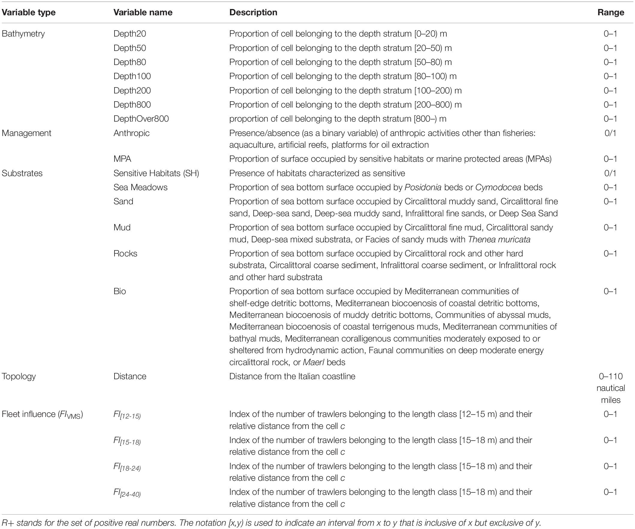
Table 1. List of input variables used for training of CMPN.

• The proportion of each cell belonging to the standard DCF depth strata (e.g., [0–20) m, [20–50) m, [50–80) m, [80–100) m, [100–200) m, [200–800) m, and over 800 m).

• The proportions of the surface with respect to the five different substrate typologies: mud; sand; rocks; and sensitive habitats such as sea meadows, maerl and coralligenous biocenosis.

• The presence/absence (as a binary variable) of anthropic activities other than fishing. In this study, some “direct” human activities were considered (e.g., aquaculture, artificial reefs, and platforms for oil extraction), whereas indirect activities (e.g., pollution) were not considered.

• The proportion of the surface area occupied by MPAs.

The Fleet of Trawlers and Its Datasets

The official fleet of Italian trawlers operating in the Adriatic Sea consists of 2,207 vessels (Table 2). Vessels belonging to the length class [12–15 m), i.e., the subset not mandatorily equipped with the VMS/AIS, represents 74.17% of the total. Fleet segments corresponding to the length classes [15–18 m), [18–24 m), and [24–40 m) were comprised almost entirely of vessels equipped with VMS. The VMS data were made available by the Italian Ministry of Agricultural, Food and Forestry Policies within scientific activities related to the Italian National Program for Data Collection in the Fisheries Sector. The VMS data consist of pings sent at regular frequencies from vessels, regardless of their status (i.e., fishing, steaming, or other). Standard procedures exist to organize, clean, interpolate and classify the VMS data (Russo et al., 2011a,b, 2014a, 2016b). In brief, VMS data can be used to compute the amounts and locations of trawling efforts, definitively allowing reconstruction of the fishing activity for each vessel at a given temporal or spatial scale.

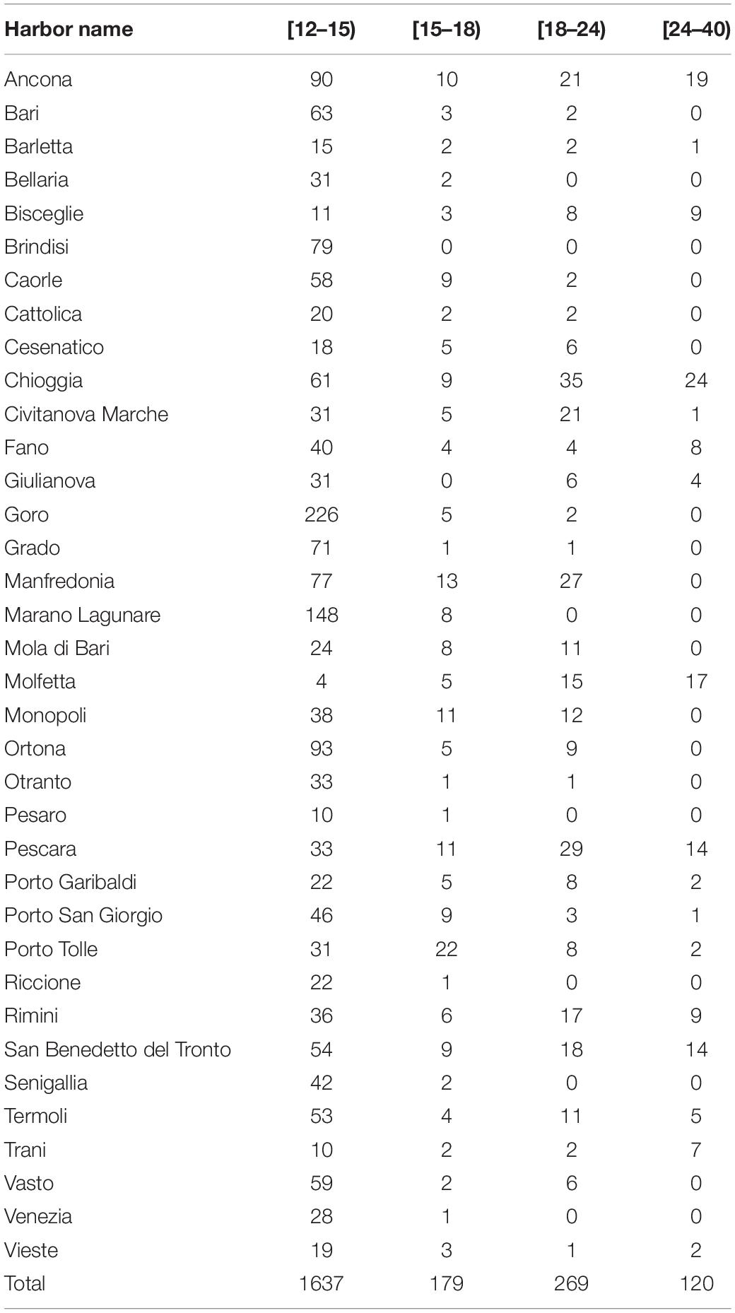
Table 2. Number of trawlers for each Italian harbor along the Adriatic coast and for each length class according to the DCF.

In addition, a set of logbook data covering the activity of 39 Adriatic trawlers belonging to the length class [12–15 m) for the whole year of 2017 was provided. Each record in this logbook dataset contains data arranged by vessel and by fishing day and shows the amount of effort (in hours) and the mean geographical locations (centroids) of fishing activities. It is worth noting that none of these 39 vessels was equipped with the VMS. This lack of a VMS implies that these trawlers represent a completely independent dataset that does not overlap with the trawlers previously described.

Fishing Effort

The yearly fishing footprint was estimated from the VMS data for the years 2012–2016 in terms of the grid defined above for each fleet segment, using the procedure described in Russo et al. (2011a, b, 2014a, 2016b). The fishing effort was quantified as hours of fishing for each fleet segment, regardless of the engine power of the fishing vessels or the gear widths (which are generally related to the vessel size – Reid et al., 2011).

The corresponding means across years 2012–2016 are shown in Figure 3. These mean patterns were then used as input for the model (see the next sections). A preliminary analysis of the Pearson correlations between these patterns (Figure 4) enabled the detection of positive interactions, e.g., between the fleet segments [15–18 m) and [18–24 m), and of negative interactions (repulsion), e.g., between segments [15–18 m) and [24–40 m).

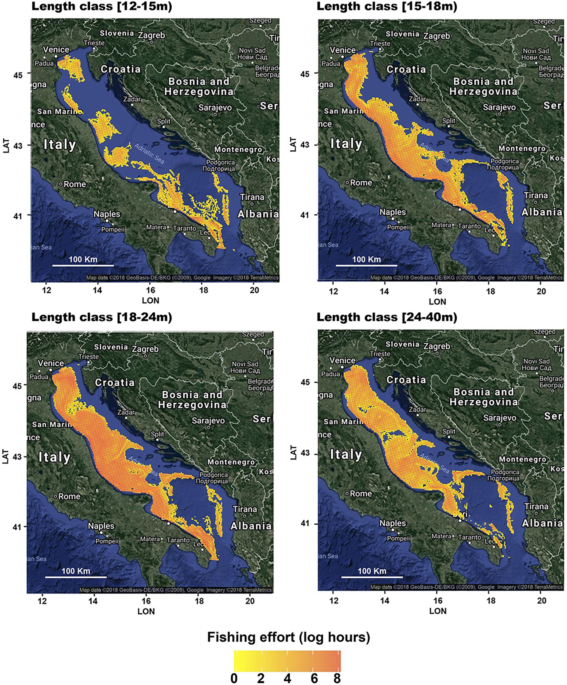
Figure 3. Fishing footprints as the total yearly fishing effort (the means of the years from 2012 to 2016), estimated using the VMS data, for the four length classes that group the Italian trawlers operating in the Adriatic Sea. The effort in the logs of fishing hours was computed with respect to the 3 × 3 km square grid used within the EU DCF for the computation of the ecological indicators of fishing pressure. The effort scale is the same for the four subfigures to provide comparability. The figures were created using the R package ggmap (Kahle and Wickham, 2013) importing images from Google maps.

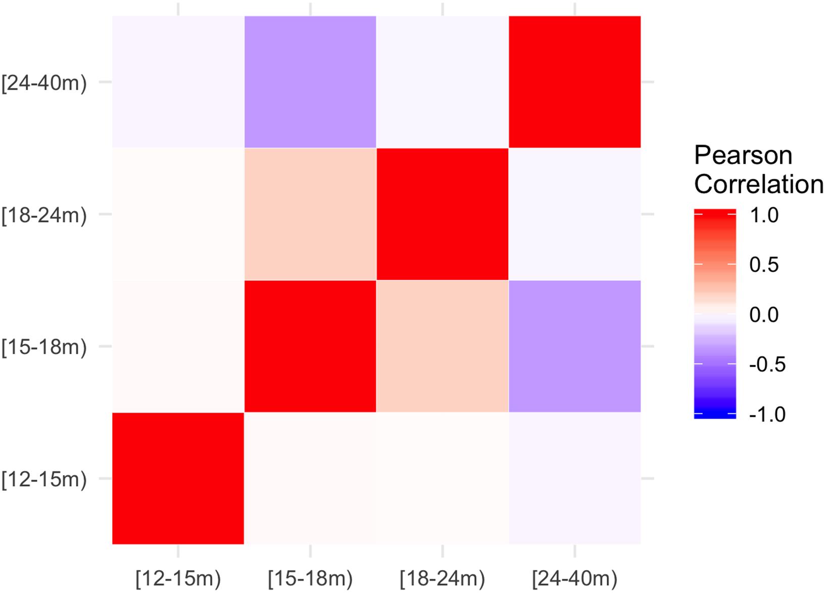
Figure 4. Visualization of the Pearson Correlation between the fishing efforts observed for the different length classes, as estimated by the VMS data. Correlation values are represented with a color scale ranging from blue (negative) to red (positive) values. The fleet segments are named according to the ranges of length-over-all of the vessels. The notation [x,y) is used to indicate an interval from x to y that is inclusive of x but exclusive of y.

After model training, a second block of estimates was produced. In particular, the model described in the next sections was used to predict the fishing footprints for the year 2017 for each fleet segment, considering the official size of each segment.

In addition, the yearly aggregated fishing footprint for the year 2017 for the 39 vessels in the logbook dataset was predicted. At the same time, the corresponding fishing footprint for these vessels was computed using the logbook data. That is, the daily amount of trawling effort was assigned to the grid cells using the information of the centroids of fishing activity for each day.

The model predictions and logbook-based assessments were then compared (see section “Model Validation and Sensitivity Analysis”).

Fishing Capacity and Fleet Distributions

It is reasonable that the trawling effort deployed within a given cell is a function of the cell characteristics and of its position with respect to harbors. In other words, the steaming distance to reach a given cell is a critical factor and, in theory, the attractiveness of a given cell is expected to be inversely correlated to its distance from the starting harbor for each vessel. Conversely, trawling effort deployed in a given cell should be positively influenced by the fleet size (i.e., the number of trawlers belonging to different fleet segments) distributed in the nearest harbors. In brief, the trawling efforts are likely to be influenced by the system topology. However, trawlers belonging to different length classes are likely to be characterized by different operating ranges.

To model these relationships, the distances between each Italian harbor on the Adriatic coast hosting trawlers (Table 2) and the centers of each cell c were computed and combined with the trawler distributions by harbor and length class to obtain the “fleet influence” (FI_c,l) index, defined as:

where c is a generic cell, l is a standard DCF length class for LOAs (12–15 m), (15–18 m), (18–24 m), and (24–40 m), d_c,h is the distance between cell c and harbor h, and N_h,l is the number of trawlers hosted in harbor h and belonging to length class l.

The largest values of the FI index occur for cells near harbors hosting the largest fleets of trawlers. Conversely, the lowest values (corresponding to no influence on the fleets) occur for cells at a distance from harbors inversely correlated to the size of the hosted fleets.

Three separate sets, each composed of four vectors (one for each length class), were computed for FI. The first set (FI_CFR) was computed considering the official (i.e., total) number of trawlers by harbor/length class (Table 2) according to the CFR. The resulting patterns are represented in Figure 5. The second set (FI_VMS) was computed considering only the trawlers equipped with the VMS (i.e., those for which the fishing footprints could be directly estimated). The third set (FI_LB) was computed considering only the 39 trawlers in the logbook dataset.

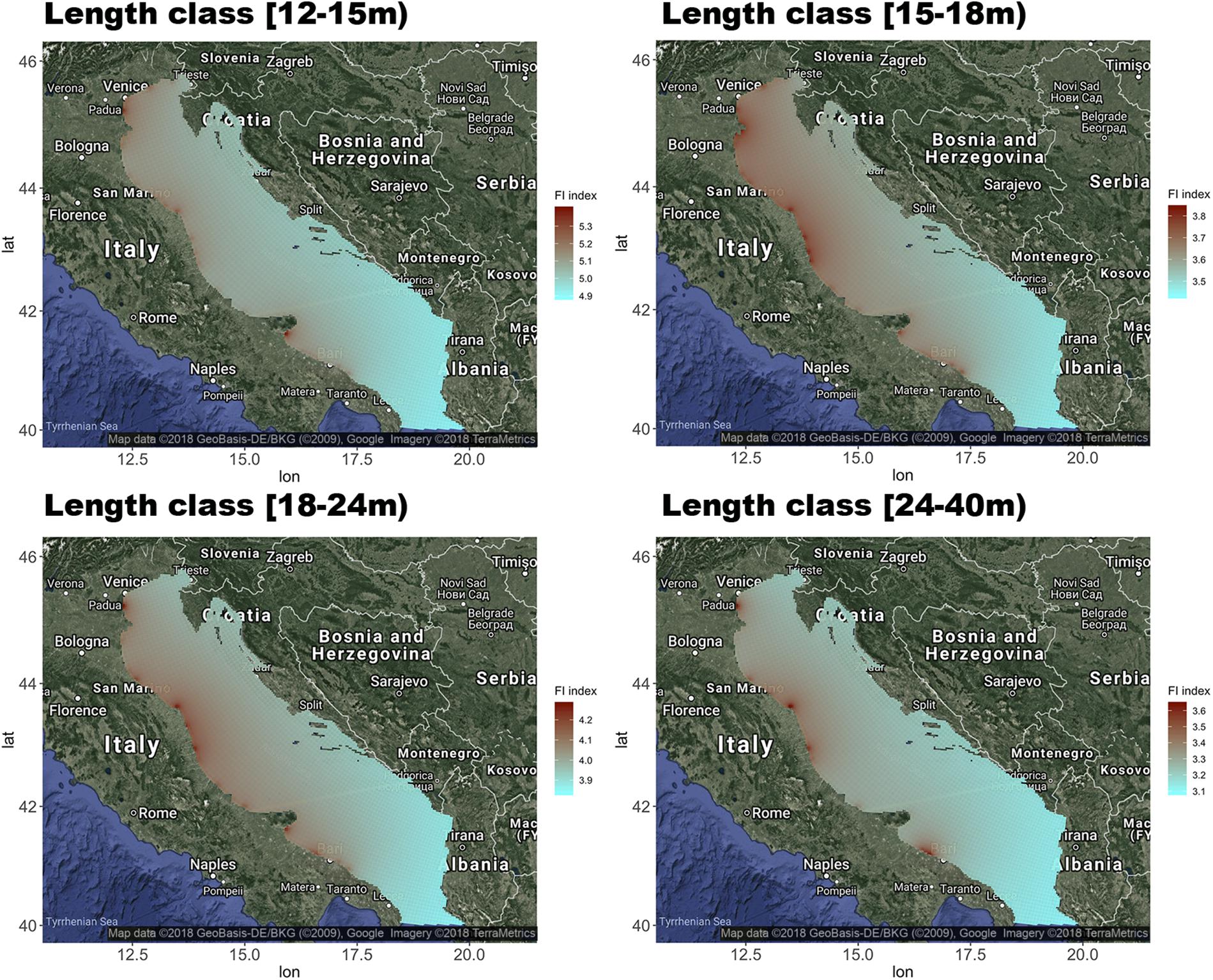
Figure 5. Spatial patterns of the FI index, by length class, computed considering the official (i.e., total) number of Italian trawlers by harbor/length class (Table 2). The FI index is defined as a function of the size of the fleet segment (i.e., the number of trawlers) and the distance from the center of each cell to the harbor. The figures were created using the R package ggmap (Kahle and Wickham, 2013) importing images from Google maps.

Rationale of the Model and Structure of the Cascaded Multilayer Perceptron Network

The model presented in this study aims to predict the yearly fishing efforts (FE_c,l), as hours of fishing, for each fleet segment l and for each cell c in a set of C cells, starting with the VMS data for a subset of these vessels. We can assume that the effort spent by each fleet segment in a given cell depends on a set of covariates related to the cell. Moreover, it is reasonable to assume that it also depends on the effort spent by all other fleet segments. For example, vessels of similar lengths will have similar behaviors, while an extensive effort by large vessels will discourage smaller vessels. This assumption is corroborated by the correlations shown in Figure 4. Hence, instead of estimating a model for each segment, we employ a joint model for the efforts of all segments.

If we used the whole dataset, we could estimate the joint model using a MPN. For this setup, we cannot estimate the model in a single step. Instead, we impute the missing data in the first step, and then estimate the whole model during the second step.

To accomplish this task, a CMPN was defined to predict the values of FE_c,l. The CMPN presented in this study (Figure 6) consists of two MPNs. Each MPN belongs to the ANN family of “feed-forward” neural networks, which is the oldest and simplest ANN type (Quetglas et al., 2011). This ANN family is composed of three strata of “neurons,” and the information conveyed by the training data flows only in the forward direction, from left (input stratum) to right (output stratum), passing through “hidden” neurons (intermediate stratum). Each neuron of the input stratum is connected to all neurons of the hidden stratum, and each neuron of the hidden stratum is connected to all neurons of the output stratum. No connections are present between neurons of the same stratum. The number of neurons in the input stratum corresponds to the number of independent variables or descriptors employed to predict the dependent variables, which correspond to the neurons in the output stratum. The intermediate (hidden) stratum, the core of the MPN, contains a variable number of neurons, since the size of this layer is a parameter to be tuned when optimizing the MPN structure. Each neuron in this stratum computes, through a first “activation” function, a weighted sum of values in the input layer. Then, the neuron swaps this intermediate value to output neurons through a second activation function. In this study, a sigmoid function (the most common choice in this field – Lek and Guégan, 1999; Haykin and Haykin, 2009) was used in both cases.

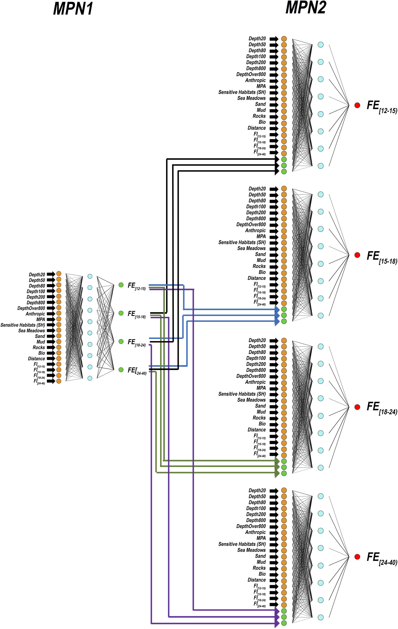
Figure 6. Structure of the cascaded multilayer perceptron network used in this study. The names of the input variables are shown on the left side. The MPN in the first layer has four output neurons, one for each FE_c,l of a given l length class. The MPNs in the second layer has one output neuron each, since they processes FE_c,l from MPN in layer one by considering interactions between fleet segments. Different colors of input neurons are used to emphasize the fact that MPNs in the second layer reuse input data for MPN in the layer one (orange) plus their outputs (green). The neurons in the hidden strata are represented in cyan. Final output neurons are in red.

The classic MPN training procedure is based on a dataset for which both the independent and dependent variables are known and consists of adjusting the connection weights among neurons of different strata to minimize the discrepancies between the observed and predicted values (Quetglas et al., 2011). At the end of the optimization process, the connection weights among the neurons of different strata are kept fixed, and a different dataset (not previously used for the training phase) can be used for testing. In this way, new sets of values for the input descriptors are used to feed the trained MPN, and the predicted values of the dependent variables are compared with the observed values to assess the ability of the MPN to model the phenomena of interest. The CMPN architecture applied in this study consists of two MPNs (Figure 6), named MPN1 and MPN2. MPN1 consists of 20 neurons in the input stratum, which correspond to the variables shown in Table 1. The output stratum of MPN1 consists of four neurons, corresponding to the FE_c,l values described above. According to this architecture, the aim of MPN1 is to model the effects of the different groups of independent variables (bathymetry, management, substrates, topology and fleet influence) on the fishing efforts for the four length classes (output variables FE_c,l) but spatial interactions between the output variables are not considered. In other words, MPN1 is not intended to take into account the interactions between the components of the fleet that correspond to the different length classes (Figure 4). This fact is the reason why a second MPN ensemble (MPN2 in Figure 6) was designed. Each MPN2 uses the same set of 20 independent variables that feed MPN1, along with three of the four sets of FE_c,l values returned by MP1, to refine FE_c,l predictions of the fourth. Thus, each MPN2 has a single output neuron. CMPN has been applied in other ecological studies when a correlation exists among output variables (Franceschini et al., 2018).

The above described CMPN was trained and tested as follows:

1. Input variables: A subset of the 8,842 cells of the 3 × 3 km grid was defined after exclusion of the Croatian territorial waters and after exclusion of the cells closer than 3 km to the Italian coastline. The values for the 20 independent variables (Table 1) plus the mean total yearly fishing efforts by length class were estimated for each cell.

2. Output variables: A subset of vessels with VMS was extracted from the CFR and the corresponding values of FE_c,l were computed.

3. Both input and output quantitative variables were normalized in the range [0–1], while the qualitative variables (anthropic activities and sensitive habitats) were expressed as presence/absence binary values (0/1).

4. The training phase of an MPN is typically carried out using two input datasets (the training set and the validation set), since this allows limiting the risk of “overfitting,” but a test dataset is used to assess the performance of the trained MPN. Overfitting occurs when the model fits the observed data too well and is not able to effectively generalize the phenomena of interest, leading to poor predictive performance for the test dataset. The risk of overfitting is particularly high in spatial models (Black, 1995) because neighboring spatial units are likely to be very similar. To minimize the effect of spatial autocorrelation, the set of 8,842 cells and their corresponding input and output variables were first partitioned into 45 blocks, each defined as a group of cells within a square box of 0.75 × 0.58 degrees (Figure 7A). Then, 70% of those blocks were randomly selected for the training set, 15% of the blocks not assigned to the training set were randomly selected for the validation set and, finally, the remaining 15% not attributed to either the training set or to the validation set were used as the test set (see section “Model Validation and Sensitivity Analysis”).

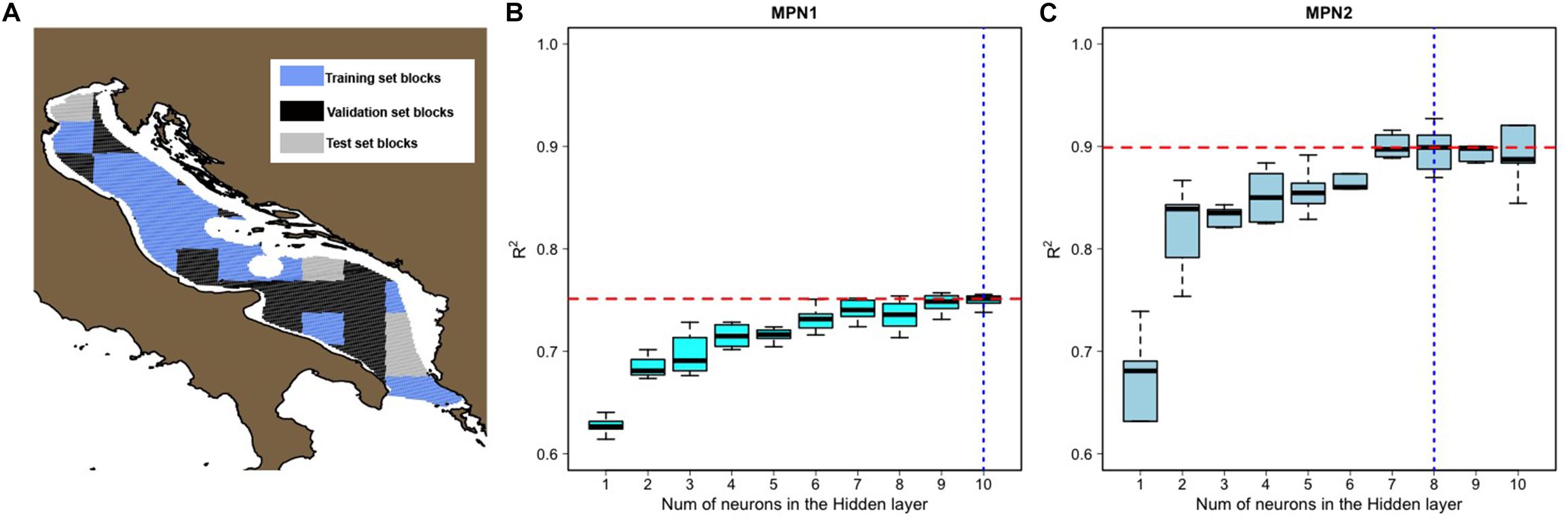
Figure 7. (A) Example of the random definition of blocks for the training, validation and test datasets. Performance (measured as R² values between the predicted and observed values of the fishing effort in the test dataset) of MPN1 (B) and MPN2 (C) with different numbers of neurons in the hidden stratum. The entire training and test procedure, including random partitioning of data in training and test sets, was replicated 10 times for each value of the number of neurons in the hidden stratum. For MPN2, the distributions in the boxplots represent the aggregation of the four MPN2s (one for each length class). The dashed blue lines in (B) and (C) indicate the selected values of the number of neurons in the hidden stratum. The dashed red lines in (B) and (C) provide the corresponding median R² values for MPN1 and MPN2 with the selected values of the number of neurons in the hidden stratum.

5. The training, validation and test datasets were used to optimize the number of neurons in the hidden layer of MPN1. The values between 1 and 10 neurons were explored by repeating dataset extractions (step 4 in this list) 10 times for each value and then by assessing MPN1 performance by comparing the predicted values of FE_c,l for the test dataset with the observed values through the determination coefficient R².

6. After the identification of the optimal number of neurons in the hidden stratum of MPN1, the same procedure was successively applied to optimize the size of the hidden stratum for the MPN2s.

7. At the end of optimization phase for both MPN1 and MPN2, the final structure of the CMPN was defined.

Model Validation and Sensitivity Analysis

The performance of the optimized CMPN was first assessed by means of a cross-validation (CV) procedure. CV is a popular technique for model evaluation. CV is based on random partitioning of available data in different and non-overlapping subsets. The subsets not used for training, commonly called “test” datasets, are submitted to the trained model. Then, model predictions are compared with observed values for the test dataset to assess the goodness of model fit (Kärkkäinen, 2014). In practice, the resampling procedure described in the previous section (step 4) was repeated 100 times, generating 100 training (70% of cells), validation (15% of cells), and test (15% of cells) datasets. Then, after model training, the CMPN predictive performance was measured by comparing the predicted values of FE_c,l for the cells in the test dataset with the observed values using the determination coefficient.

Moreover, the ability of the model to predict the spatial effort patterns of trawlers belonging to the fleet segment [12–15 m) was evaluated using the ancillary logbook dataset (39 trawlers distributed in 11 Adriatic harbors), which provided an independent data source. The agreement between these two patterns was evaluated as follows: (1) the continuous values of fishing efforts by cell were discretized into classes; (2) a confusion matrix (Stehman, 1997) was generated by comparing the two classifications (CMPN-based predictions and logbook-based observations); and (3) this matrix was analyzed by means of the weighted Cohen’s kappa statistics (Cohen, 1968) using the function cohen.kappa in the R package “psych” (Revelle, 2019).

As explained in section “Rationale of the Model and Structure of the Cascaded Multilayer Perceptron Network,” the MPN outputs depend upon both input variables and connection weights in the hidden stratum, so an important issue is the model sensitivity to perturbations in these values. Here, sensitivity means the amount of change in the output values as determined by changes of inputs or weights. This structural characteristic of MPN can be used to evaluate the relative influence of the input variables: if the values of a single input variable are changed (while those for the other input variables are kept the same) it is possible to observe the related effects on the outputs. Therefore, if this procedure is applied, for each input variable, by perturbing the input values at defined levels, the comparisons of the effects on the output values can be used to assess the relative influence (importance) of the input variables (Scardi and Harding, 1999; Franceschini et al., 2018). Hence, to evaluate the contributions of the independent variables to the prediction accuracies, a set of perturbation levels [initial values⁵ ±0.1, ±0.2, ±0.3, ±0.4, and ±0.5] was applied, and the related effects on the output values were measured as the mean square errors (MSE) of the CMPN outputs with respect to the values in the test datasets.

Results

The best performances (R²) of MPN1 and MPN2 were 0.75 and 0.89, respectively. It is worth noting that these values of agreement were obtained for the test datasets, which do not overlap with either the training or validation datasets used during the learning phase. However, both MPN1 and MPN2, with similar numbers of neurons in the hidden layer, returned similar values of R², providing evidence of training stability (Figure 7). A CMPN with 10 neurons in the hidden stratum of MPN1 and 8 neurons in the hidden stratum of MPN2 (CMPN_10–8 hereafter) returned the best results in terms of R² between the predicted and observed values for the test datasets (Figure 8). According to these results, CMPN_10–8, was selected and used for the rest of the analyses.

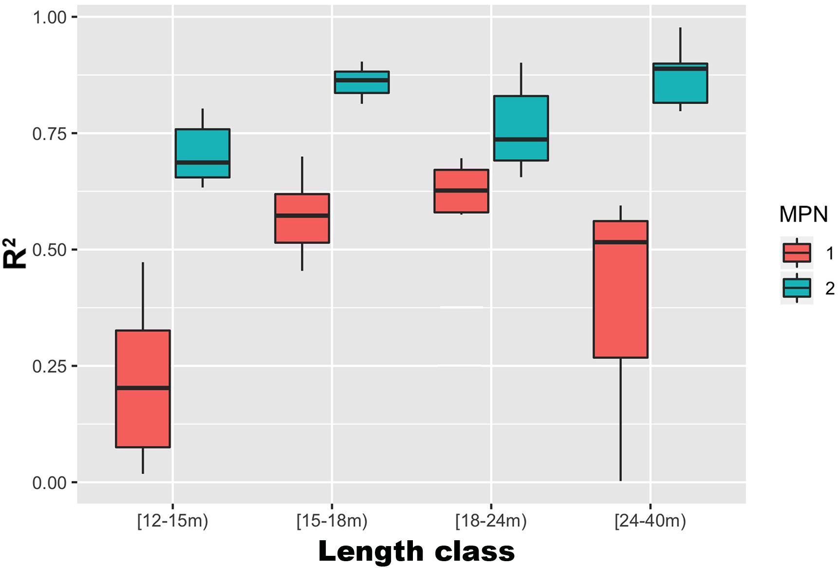
Figure 8. Boxplots of the MPN1 (red) and MPN2 (blue) performances (R² between predicted and observed fishing efforts for the test datasets, using 100 random repetitions) of the CMPN_10–8 (the CMPN with 10 neurons in the hidden stratum of MPN1 and 8 neurons in the hidden stratum of MPN2, which scored as the best architecture). Boxes and whiskers showing the medians (thick lines), 25th and 75th quantiles (lower and upper margin of the boxes) and ranges (vertical lines) of values.

The detailed analysis of CMPN_10–8 performances for the different length classes (Figure 7) indicates that MPN1 performed better for the intermediate length classes. The MPN2s, however, returned high and homogeneous performances for length classes [15–18 m) and [18–24 m), whereas the performance for length classes [12–15 m) and [21–40 m) were lower and much more variable. However, the mean R² for MPN2 was 0.77 ± 0.048 (mean ± standard deviation). R² values ranged from 0 to +1 and measured how well the observed patterns were replicated by the model, based on the proportion of the total variation of observed patterns explained by the model. In this manner, the R² values obtained for CMPN_10–8 indicated that it was able to capture approximately 80% of the variability in the observed data.

CMPN_10–8 was then used to predict the distribution of the fishing effort for the whole fleet, according to the procedure described in sections “Fishing Capacity and Fleet Distributions” and “Rationale of the Model and Structure of the Cascaded Multilayer Perceptron Network,” that is, by replacing FI_VMS with FI_CFR in the input variables of both MPN1 and MPN2s. It is worth noting that, while the values of FI_VMS and FI_CFR were very close for fleet segments [15–18 m), [18–24 m), and [24–40 m), they are substantially different for the fleet segment [12–15 m). This finding was determined by the low percentage of vessels with VMS in the length class [12–15 m) (see Figure 1) and implies that the application of CMPN_10–8 on FI_CFR for this fleet segment corresponds to an expansion of the behavior (in terms of the spatial deployment of fishing effort) of vessels with the VMS to the whole fleet.

The patterns obtained for the different length classes are represented in Figure 9. While the patterns for length classes [15–18 m), [18–24 m), and [24–40 m) were very similar to the observed patterns (Figure 3), those for length class [12–15 m) depicted, as expected, an exploited area that was much wider than the observed area. In terms of fishing grounds, the pattern for length class [12–15 m) was characterized, first, by a high level of effort along the Italian coast, especially in GSA17, with the exception of a large area offshore from Ancona. Some fishing grounds far from the Italian coast were also represented: one fishing ground was in front of Istria’s peninsula (Croatia), one fishing ground was in front of Split (Croatia), and the band-shaped fishing ground was in front of Montenegro’s coasts.

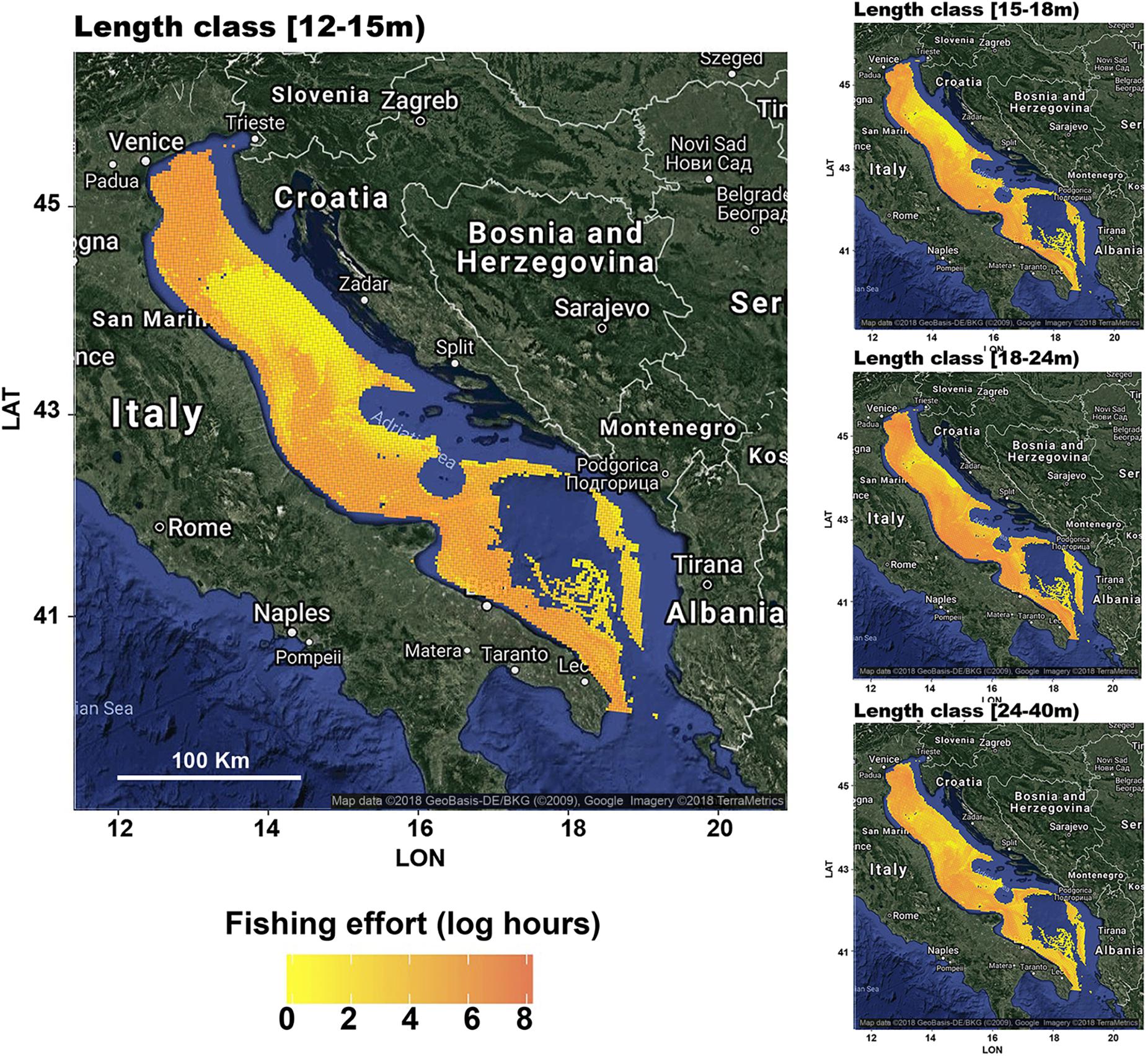
Figure 9. Fishing footprints as the total yearly fishing efforts (means of the years 2012–2016) estimated from CMPN_10–8, for the four different length classes that group the Italian trawlers operating in the Adriatic Sea. Particular emphasis is given to the length class [12–15 m). The effort scale is the same for the four subfigures to provide comparability. The figures were created using the R package ggmap (Kahle and Wickham, 2013) importing images from Google maps.

The comparison of the fishing footprints (as the total fishing effort in the year 2017) predicted by CMPN_10–8, using FI_LB and the corresponding pattern computed from the logbook data is presented in Figure 10. The value of the weighted Cohen’s kappa computed for this pattern was 0.79, which implies substantial agreement (Cohen, 1960). In fact, a visual inspection of these patterns shows strong similarities, especially in the southern part of the Adriatic Sea (GSA18). The main differences between the predicted and observed patterns were detected in GSA17 (Northern portion of the Adriatic Sea). In particular, CMPN_10–8 predicted fishing efforts along the entire Italian coast, whereas the logbook data recorded fishing activity in three fishing grounds: a large area near Venice, a small area near San Marino and another large fishing ground in the southern part of GSA17. In addition, the logbook data revealed fishing activities near Split and near the coast of Albania.

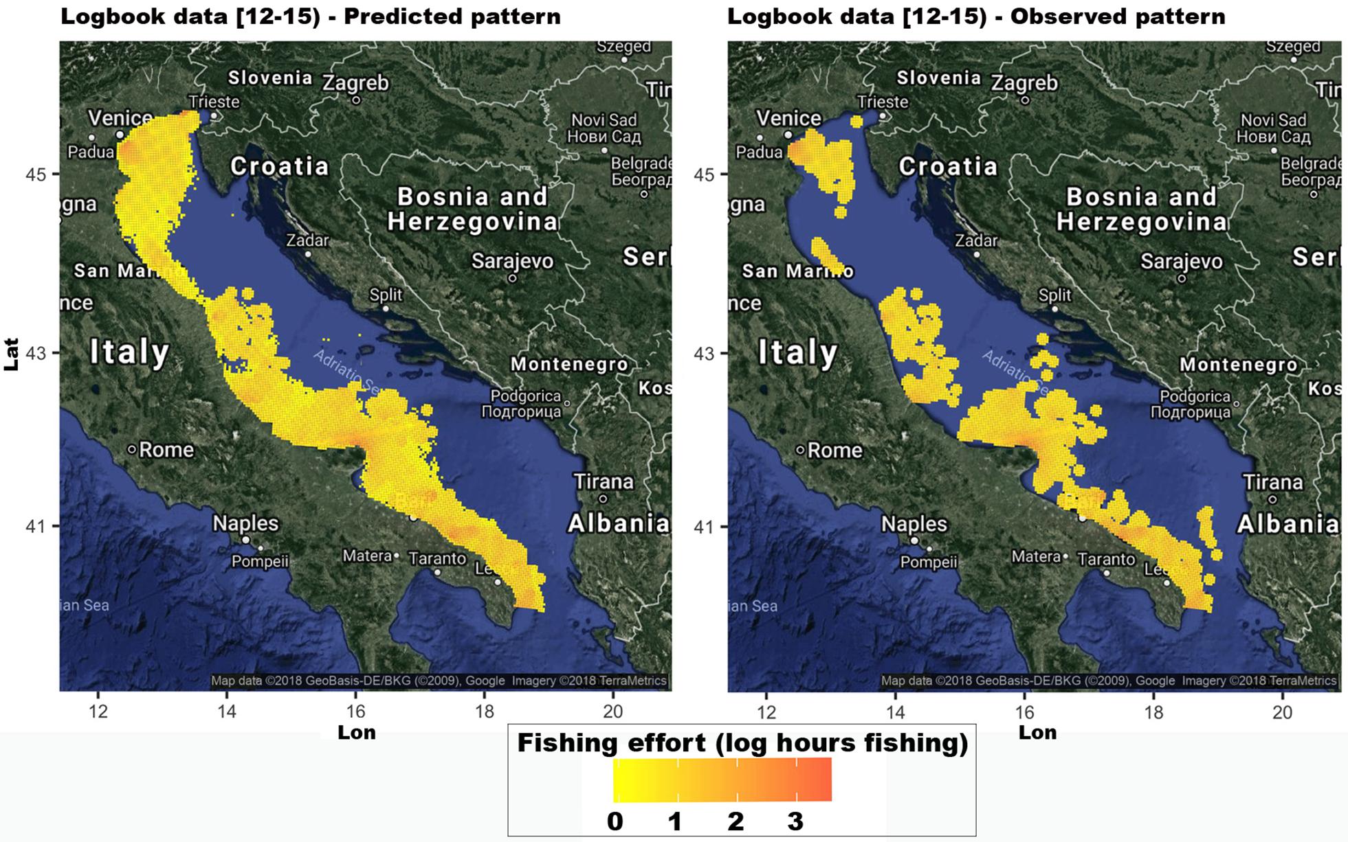
Figure 10. Comparison of the fishing footprint (as the total fishing effort in the year 2017) predicted (left) by the CMPN_10–8, for the 39 vessels in the logbook dataset and the corresponding pattern (right) computed from the logbook data. The figures were created using the R package ggmap (Kahle and Wickham, 2013) importing images from Google maps.

The outputs of the sensitivity analyses (Figure 11) showed that there is a large set of variables that influence the outputs for length class [12–15 m), whereas only a few input variables were relevant for the other three length classes. The effort of the adjacent higher length class is the most important input variable for length classes [12–15 m) and [15–18 m). Conversely, the effort of the length class [15–18 m) is the most important input variable for the length class [12–15 m). The distance from the coast has the main effect on the predicted fishing footprints for length class [24–40 m). With the exception of effort [15–18 m) for length class [12–15 m), the variations in MSE were proportional to the perturbations.

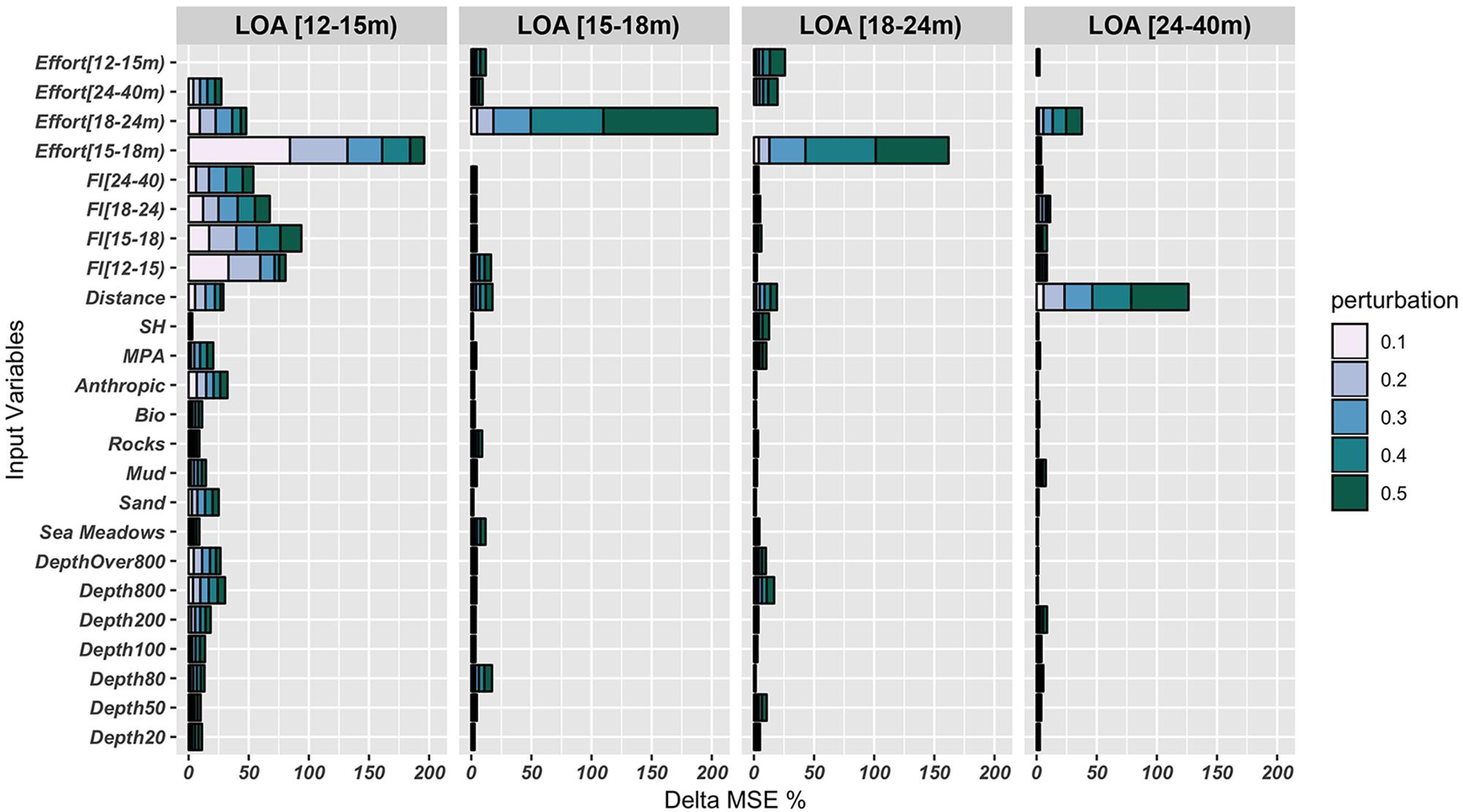
Figure 11. Outputs of the sensitivity analyses based on the perturbation method. This procedure was applied for each input variable, by perturbing the input values at defined levels [initial values ±0.1, ±0.2, ±0.3, ±0.4, and ±0.5], and then exploring the related effects on the output variables in terms of mean square error (MSE) between the predicted and observed values for the test. Bar lengths (x-axis) represent the increase in the mean square error (MSE) of the CMPN_10–8 outputs obtained by perturbing each of the input variables in the test datasets, while keeping all other inputs at their original values, and are presented as stacked bars in which the color scale describes the size of the perturbation.

Among the variables influencing the prediction for length class [12–15 m), those describing fleet structure (FI index) were the most important, followed by the distances from the coast, the presence of anthropic activities in addition to fisheries, MPA, percentages of sea bottom classified as “sand” and depth stratum.

Discussion

Reconstructing fishing efforts in space and time is a prerequisite for fisheries management and a critical step toward an ecosystem approach to fisheries, since it is largely acknowledged that fishing represents one of the most impactful human activities (Collie et al., 2000; Smith, 2000; Kaiser et al., 2002). In the last decade, the progressive application of tracking devices (e.g., the VMS and AIS) has provided managers and scientists with data of high spatial and temporal resolution, which represent, in combination with other data (e.g., satellite estimates of primary production and distribution of stocks by genetic data) the basis for advanced models of resource exploitation (Gerritsen and Lordan, 2011; Bastardie et al., 2014; Russo et al., 2014b). These models ultimately support monitoring and forecasting of fishing-related impacts and allow simulating the effects of management approaches based on regulation of fishing efforts. Moreover, leaving aside issues related to fishing safety and enforcement (e.g., control of access to fisheries-restricted areas), the VMS/AIS-based quantification of the fishing efforts and fishing strategies is a natural consequence of the awareness that the sea and its resources are common goods and those who extract from them should be monitored (Fournier et al., 2018). However, vessels and fleets without a VMS or AIS are practically able to operate in “hidden mode,” and reconstructing their activities and related impacts is challenging. All of these considerations apply to the Mediterranean Sea, one of the most exploited large marine ecosystems worldwide, and in particular to the Adriatic Sea, in which trawling efforts have reached the highest levels on the entire planet even when the contribution of trawlers belonging to fleet segment [12–15 m) is not considered (Amoroso et al., 2018). In summary, the estimation of the fishing footprints of vessels without the VMS or AIS is urgent and strategic.

The results of this study suggest that a CMPN is a suitable tool to pursue this aim. The CMPN_10–8 designed and trained on VMS data for a subset of vessels belonging to length class [12–15 m) returned an estimate of the total annual fishing effort for the whole Italian fleet in this fleet segment. The model outputs were validated in two ways: internally (CV using test data not used for training – see Figure 8) and externally (i.e., through comparison with independent estimations from logbook data – see Figure 10). The latter type of validation, in particular, indicated a substantial agreement between the model output and the patterns depicted by the logbook data. The discrepancies between the model output and the logbook-based patterns can be explained in different ways. First, of course, these discrepancies could be related to model limitations in terms of predictive power. If this is the case, it is worth noting that the model was trained with VMS data for approximately 3% of the whole fleet in the length class [12–15 m) (see Figure 1). Therefore, the model output should be judged while considering that the model predictions were based on a small subset of the target universe. Moreover, it is reasonable to expect that the model performance will improve with the progressive coverage of the VMS (or AIS) for this fleet segment. Second, mismatches between model outputs and logbook-based patterns could be due also to misreporting or gaps in the logbook data. In fact, logbooks are characterized by consistency and accuracy issues (Chang, 2011; Sampson, 2011; Russo et al., 2016a). Beyond these inconsistencies, the model presented in this paper represents one of the first attempts to apply ANN to extrapolate the behavior of entire fleets from subsets of these fleets. Hence, the target of the model is represented by an aggregated (yearly) pattern rather than high-resolution temporal scales (trips or days). This fact is also related to the rationale of the model; we are not modeling the behavior of each vessel (i.e., where and how much it operates). In contrast, we are trying to model (and predict) the effort allocated in a given spatial unit (cell) as a function of its environmental characteristics and its position with respect to the system topology of the structure/distribution of the fleet.

The fishing footprint predicted by the CMPN for length class [12–15 m) looks very similar, in terms of the hotspots of effort and the distribution of fishing grounds, to the observed footprint (from the VMS data) for the other length classes and, in particular, for length class [15–18 m). The Adriatic Sea hosts approximately half of the Italian trawling fleet and is one of the most crowded marine areas of the world (Bastardie et al., 2017; Carpi et al., 2017); fishing vessels are forced to compete for the same fishing grounds. Here, the high productivity of mollusks, shellfish, and finfish of high commercial value causes strong competition for demersal resources (Fortibuoni et al., 2017). Trawl fishing in the Adriatic Sea is extremely productive, since it benefits from the environmental characteristics of a semi-enclosed basin, that is, a flat bottom covered by mud and sand that receives relevant nutrient outflows from the incoming rivers (e.g., mainly the Po river) (Papaconstantinou and Farrugio, 2000). Apart from the areas occupied by infrastructures that prevent fishing activities (e.g., offshore platforms for oil extraction) and the complex of the Pomo Pit, the Adriatic Sea is almost completely suitable for trawling. Consequently, areas of activity for different fleet segments depend mainly upon two factors: the different operating ranges of small/large vessels and the competition for space between the different fleet segments.

The vessel density in the fishing grounds has been inversely correlated with economic performance, so minimizing spatial overlap and competition for the same fishing grounds is considered a common strategy adopted by fishermen (Rijnsdorp, 2000). Coherently, the sensitivity analysis demonstrated that the distance from the coast is the main input variable influencing the fishing effort patterns of the largest fleet segment, which can operate far from the coast and minimize its overlap with the other fleet components. Noticeably, the fishing effort pattern for the smallest fleet segment [12–15 m) depends upon several input variables, most of which are related to substrates and the sea-bottom depth. In the same way, human activities other than fishing are relevant only for the fleet segment [12–15 m) (Figure 11). These results can be explained by considering that the environment is more variable near the coast and that aquaculture sites, artificial reefs, and platforms for oil extraction are located along the coast, with this being the region within which the efforts of this fleet segment are concentrated. In addition, this fleet segment is the largest in terms of size (i.e., total number of fishing vessels) and so the competition for fishing grounds is very strong within this segment. These results are consistent with previous studies addressing the relationships between fishing efforts and distances between ports and fishing grounds for different subsets of fleets (Rijnsdorp, 2000; Bastardie et al., 2014).

The two MPNs composing the CMPN designed in this study are explicitly aimed at considering these two different blocks of drivers that shape the fishing effort patterns: the environmental characteristics and the reciprocal interference of the different fleet segments. MPN1 basically processes the input variables of the environmental block, although the gravimetric influence of the fleet capacity stored in the harbors is also considered. However, given that the output neurons of a MPN are not connected, it cannot take into account the influence of the intersegments (Figure 5), which is instead the target of MPN2.

Future Work

Given that, (1) the aim of this study was to develop and test a method to predict fishing effort allocations for a group of vessels without tracking devices; (2) the method presented was focused on spatial units instead of on individual vessels (i.e., the output of the CMPN is the effort in a generic cell rather than the behavior of a generic vessel); and (3) the set of trawlers with VMS in the length class [12–15 m) was not large enough to support further partitioning by engine power, the different characteristics of vessels belonging to different length classes (namely, their engine power, which significantly affects the effective effort and its related impacts) were not considered. Future developments of this method, perhaps based on larger datasets, could address this issue.

From a practical point of view, the fishing effort pattern estimated for the fleet segment [12–15 m) will be used, in combination with the fishing effort patterns of other fleet segments, to define a model of trawling fisheries in the Adriatic Sea within the research project “MANTIS: Marine protected areas: network(s) for enhancement of sustainable fisheries in EU Mediterranean waters.” The project is aimed at estimating, through simulation approaches integrated into the SMART model (Russo et al., 2014b), the potential effects on the demersal resources under different management scenarios, including the creation of large areas closed to fisheries in the Pomo Pit complex (Bastari et al., 2016; Bastardie et al., 2017; Carpi et al., 2017). Considering the relevant amount of fishing effort and related catches associated with the fleet segment [12–15 m), it seems very important to take into account the interactions of fishing footprints and resource distributions with particular reference to critical life stages and living marine resources (Colloca et al., 2017).

However, this first application of CMPN was devised to estimate the annual pattern of fishing efforts, but future developments could address fine temporal scales (e.g., seasonal). This work could open up important perspectives in terms of the relationships between seasonal patterns of fishing effort and the distribution/life cycle of different demersal resources, which were not considered in this study.

It may also be relevant to address, in more detail, the role of other factors influencing the effort distribution (e.g., pollution, different fuel prices along the coast, fine scale structures of coastal communities, fishing traditions, owners and market requests).

Data Availability Statement

The datasets for this manuscript are not publicly available because VMS data are confidential. Requests to access the datasets should be directed to Tommaso.Russo@Uniroma2.it.

Author Contributions

TR, SF, LD’A, and MS conceived the ideas and designed the methodology. TR and SF collected the data and analyzed the data. TR and AP wrote the manucript. All authors contributed critically to the drafts and gave final approval for publication.

Funding

This work has been supported by the European Commission – Directorate General MARE (Maritime Affairs and Fisheries) through the Research Project “MANTIS: Marine protected areas: network(s) for enhancement of sustainable fisheries in EU Mediterranean waters (MARE/2014/41 – Ref. Ares (2015)5672134 – 08/12/2015)” and by the Ministry of Agricultural, Food, Forestry and Tourism Policies (Mipaaft) within the activities for the National Program of Data collection in the fisheries sector.

Conflict of Interest

The authors declare that the research was conducted in the absence of any commercial or financial relationships that could be construed as a potential conflict of interest.

Acknowledgments

The authors acknowledge the reviewers for their thorough and constructive criticisms, comments and suggestions.

Footnotes

1. ^ https://datacollection.jrc.ec.europa.eu/
2. ^ The notation [x,y) is used to indicate an interval from x to y that is inclusive of x but exclusive of y.
3. ^ http://ec.europa.eu/fisheries/fleet/index.cfm
4. ^ https://datacollection.jrc.ec.europa.eu/dc/fdi
5. ^ It is important to remember that each input variable was normalized to limit it to the interval [0,1].

References

Amoroso, R. O., Pitcher, C. R., Rijnsdorp, A. D., McConnaughey, R. A., Parma, A. M., Suuronen, P., et al. (2018). Bottom trawl fishing footprints on the world’s continental shelves. Proc. Natl. Acad. Sci. U.S.A. 115, E10275–E10282. doi: 10.1073/pnas.1802379115
ASOC (2011). Evolution of Footprint: Spatial and Temporal Dimensions of Human Activities. Available at: https://www.asoc.org/storage/documents/Meetings/ATCM/XXXIV/Evolution_of_Footprint.pdf (accessed October 22, 2019).
Bastardie, F., Angelini, S., Bolognini, L., Fuga, F., Manfredi, C., Martinelli, M., et al. (2017). Spatial planning for fisheries in the northern adriatic: working toward viable and sustainable fishing. Ecosphere 8:e01696. doi: 10.1002/ecs2.1696
Bastardie, F., Rasmus Nielsen, J., and Miethe, T. (2014). DISPLACE: a dynamic, individual-based model for spatial fishing planning and effort displacement — integrating underlying fish population models. Can. J. Fish. Aqua. Sci. 71, 366–386. doi: 10.1139/cjfas-2013-0126
Bastari, A., Micheli, F., Ferretti, F., Pusceddu, A., and Cerrano, C. (2016). Large marine protected areas (LMPAs) in the mediterranean sea: the opportunity of the adriatic sea. Mar. Policy 68, 165–177. doi: 10.1016/j.marpol.2016.03.010
Black, W. R. (1995). Spatial interaction modeling using artificial neural networks. J. Transp. Geogr. 3, 159–166. doi: 10.1016/0966-6923(95)00013-S
Carpi, P., Scarcella, G., and Cardinale, M. (2017). The saga of the management of fisheries in the adriatic sea: history, flaws, difficulties, and successes toward the application of the common fisheries policy in the mediterranean. Front. Mar. Sci. 4:423. doi: 10.3389/fmars.2017.00423
Chang, S.-K. (2011). Application of a vessel monitoring system to advance sustainable fisheries management–benefits received in Taiwan. Mar. Policy 35, 116–121. doi: 10.1016/j.marpol.2010.08.009
Cohen, J. (1960). A coefficient of agreement for nominal scales. Educ. Psychol. Measure. 20, 37–46. doi: 10.1177/001316446002000104
Cohen, J. (1968). Weighted kappa: nominal scale agreement provision for scaled disagreement or partial credit. Psychol. Bull. 70, 213–20.
Collie, J. S., Hall, S. J., Kaiser, M. J., and Poiner, I. R. (2000). A quantitative analysis of §shing impacts on shelf-sea benthos. Ecology 69, 785–798. doi: 10.1046/j.1365-2656.2000.00434.x
Colloca, F., Scarcella, G., and Libralato, S. (2017). Recent trends and impacts of fisheries exploitation on mediterranean stocks and ecosystems. Front. Mar. Sci. 4:244. doi: 10.3389/fmars.2017.00244
Deo, M. C. (2010). Artificial neural networks in coastal and ocean engineering. Indian J. Mar. Sci. 39:8.
Fortibuoni, T., Giovanardi, O., Pranovi, F., Raicevich, S., Solidoro, C., and Libralato, S. (2017). Analysis of long-term changes in a mediterranean marine ecosystem based on fishery landings. Front. Mar. Sci. 4:33. doi: 10.3389/fmars.2017.00033
Fournier, M., Casey Hilliard, R., Rezaee, S., and Pelot, R. (2018). Past, present, and future of the satellite-based automatic identification system: areas of applications (2004–2016). WMU J. Marit. Aff. 17, 311–345. doi: 10.1007/s13437-018-0151-156
Franceschini, S., Gandola, E., Martinoli, M., Tancioni, L., and Scardi, M. (2018). Cascaded neural networks improving fish species prediction accuracy: the role of the biotic information. Sci. Rep. 8:4581. doi: 10.1038/s41598-018-22761-22764
Gerritsen, H., and Lordan, C. (2011). Integrating vessel monitoring systems (VMS) data with daily catch data from logbooks to explore the spatial distribution of catch and effort at high resolution. ICES J. Mar. Sci. 68, 245–252. doi: 10.1093/icesjms/fsq137
Girardin, R., Hamon, K. G., Pinnegar, J., Poos, J. J., Thébaud, O., Tidd, A., et al. (2017). Thirty years of fleet dynamics modelling using discrete-choice models: what have we learned? Fish Fisher. 18, 638–655. doi: 10.1111/faf.12194
Haykin, S. S., and Haykin, S. S. (2009). Neural Networks and Learning Machines, 3rd Edn, New York, NY: Prentice Hall.
Johnson, A. F., Moreno-Báez, M., Giron-Nava, A., Corominas, J., Erisman, B., Ezcurra, E., et al. (2017). A spatial method to calculate small-scale fisheries effort in data poor scenarios. PLoS One 12:e0174064. doi: 10.1371/journal.pone.0174064
Joo, R., Bertrand, S., Chaigneau, A., and Ñiquen, M. (2011). Optimization of an artificial neural network for identifying fishing set positions from VMS data: an example from the Peruvian anchovy purse seine fishery. Ecol. Model. 222, 1048–1059. doi: 10.1016/j.ecolmodel.2010.08.039
Kaiser, M., Collie, J., Hall, S., and Poiner, I. (2002). Modification of marine habitats by trawling activities: prognosis and solutions. Fish. Fisher. 3, 114–136. doi: 10.1046/j.1467-2979.2002.00079.x
Kärkkäinen, T. (2014). “On cross-validation for MLP model evaluation,” in Structural, Syntactic, and Statistical Pattern Recognition, eds P. Fränti, G. Brown, M. Loog, F. Escolano, and M. Pelillo (Berlin: Springer), 291–300. doi: 10.1007/978-3-662-44415-3_30
Kavadas, S., Maina, I., Damalas, D., Dokos, I., Pantazi, M., and Vassilopoulou, V. (2015). Multi-criteria decision analysis as a tool to extract fishing footprints and estimate fishing pressure: application to small scale coastal fisheries and implications for management in the context of the maritime spatial planning directive. Mediterr. Mar. Sci. 16:294. doi: 10.12681/mms.1087
Lambert, G. I., Jennings, S., Hiddink, J. G., Hintzen, N. T., Hinz, H., Kaiser, M. J., et al. (2012). Implications of using alternative methods of vessel monitoring system (VMS) data analysis to describe fishing activities and impacts. ICES J. Mar. Sci. 69, 682–693. doi: 10.1093/icesjms/fss018
Lek, S., and Guégan, J. F. (1999). Artificial neural networks as a tool in ecological modelling, an introduction. Ecol. Model. 120, 65–73. doi: 10.1016/S0304-3800(99)00092-97
Léopold, M., Guillemot, N., Rocklin, D., and Chen, C. (2014). A framework for mapping small-scale coastal fisheries using fishers’ knowledge. ICES J. Mar. Sci. 71, 1781–1792. doi: 10.1093/icesjms/fst204
McCluskey, S. M., and Lewison, R. L. (2008). Quantifying fishing effort: a synthesis of current methods and their applications: quantifying fishing effort: methods review. Fish Fisher. 9, 188–200. doi: 10.1111/j.1467-2979.2008.00283.x
Natale, F., Carvalho, N., and Paulrud, A. (2015). Defining small-scale fisheries in the EU on the basis of their operational range of activity the swedish fleet as a case study. Fisher. Res. 164, 286–292. doi: 10.1016/j.fishres.2014.12.013
Papaconstantinou, C., and Farrugio, H. (2000). Fisheries in the Mediterranean. Mediterr. Mar. Sci. 1:5. doi: 10.12681/mms.2
Quetglas, A., Ordines, F., and Guijarro, B. (2011). “The use of artificial neural networks (ANNs) in aquatic ecology,” in Artificial Neural Networks - Application, ed. C. L. P. Hui (London: InTech)Google Scholar
Reid, D. G., Graham, N., Rihan, D. J., Kelly, E., Gatt, I. R., Griffin, F., et al. (2011). Do big boats tow big nets? ICES J. Mar. Sci. 68, 1663–1669. doi: 10.1093/icesjms/fsr130
Revelle, W. (2019). Package ‘psych’: Procedures for Psychological, Psychometric, and PersonalityResearch. Available at: https://cran.r-project.org/web/packages/psych/psych.pdf (accessed October 22, 2019).
Rijnsdorp, A. (2000). Effects of fishing power and competitive interactions among vessels on the effort allocation on the trip level of the dutch beam trawl fleet. ICES J. Mar. Sci. 57, 927–937. doi: 10.1006/jmsc.2000.0580
Russo, T., Carpentieri, P., Fiorentino, F., Arneri, E., Scardi, M., Cioffi, A., et al. (2016a). Modeling landings profiles of fishing vessels: an application of self-organizing maps to VMS and logbook data. Fisher. Res. 181, 34–47. doi: 10.1016/j.fishres.2016.04.005
Russo, T., D’Andrea, L., Parisi, A., Martinelli, M., Belardinelli, A., Boccoli, F., et al. (2016b). Assessing the fishing footprint using data integrated from different tracking devices: issues and opportunities. Ecol. Indic. 69, 818–827. doi: 10.1016/j.ecolind.2016.04.043
Russo, T., D’Andrea, L., Parisi, A., and Cataudella, S. (2014a). VMSbase: an R-package for VMS and logbook data management and analysis in fisheries ecology. PLoS One 9:e100195. doi: 10.1371/journal.pone.0100195
Russo, T., Parisi, A., Garofalo, G., Gristina, M., Cataudella, S., and Fiorentino, F. (2014b). SMART: a spatially explicit bio-economic model for assessing and managing demersal fisheries, with an application to italian trawlers in the strait of sicily. PLoS One 9:e86222. doi: 10.1371/journal.pone.0086222
Russo, T., Parisi, A., and Cataudella, S. (2011a). New insights in interpolating fishing tracks from VMS data for different métiers. Fisher. Res. 108, 184–194. doi: 10.1016/j.fishres.2010.12.020
Russo, T., Parisi, A., Prorgi, M., Boccoli, F., Cignini, I., Tordoni, M., et al. (2011b). When behaviour reveals activity: assigning fishing effort to métiers based on VMS data using artificial neural networks. Fisher. Res. 111, 53–64. doi: 10.1016/j.fishres.2011.06.011
Sampson, D. (2011). The accuracy of self-reported fisheries data: oregon trawl logbook fishing locations and retained catches. Fisher. Res. 112, 59–76. doi: 10.1016/j.fishres.2011.08.012
Scardi, M. (2001). Advances in neural network modeling of phytoplankton primary production. Ecol. Model. 146, 33–45. doi: 10.1016/S0304-3800(01)00294-290
Scardi, M., and Harding, L. W. (1999). Developing an empirical model of phytoplankton primary production: a neural network case study. Ecol. Model. 120, 213–223. doi: 10.1016/S0304-3800(99)00103-109
Schulz, M., and Matthies, M. (2014). Artificial neural networks for modeling time series of beach litter in the southern north sea. Mar. Environ. Res. 98, 14–20. doi: 10.1016/j.marenvres.2014.03.014
Smith, C. (2000). Impact of otter trawling on an eastern mediterranean commercial trawl fishing ground. ICES J. Mar. Sci. 57, 1340–1351. doi: 10.1006/jmsc.2000.0927
Stehman, S. V. (1997). Selecting and interpreting measures of thematic classification accuracy. Remote Sens. Environ. 62, 77–89. doi: 10.1016/S0034-4257(97)00083-87
Thiault, L., Collin, A., Chlous, F., Gelcich, S., and Claudet, J. (2017). Combining participatory and socioeconomic approaches to map fishing effort in small-scale fisheries. PLoS One 12:e0176862. doi: 10.1371/journal.pone.0176862
Watts, M., and Worner, S. (2008). Comparing ensemble and cascaded neural networks that combine biotic and abiotic variables to predict insect species distribution. Ecol. Inform. 3, 354–366. doi: 10.1016/j.ecoinf.2008.08.003
Yáñez, E., Plaza, F., Gutiérrez-Estrada, J. C., Rodríguez, N., Barbieri, M. A., Pulido-Calvo, I., et al. (2010). Anchovy (Engraulis ringens) and sardine (Sardinops sagax) abundance forecast off northern chile: a multivariate ecosystemic neural network approach. Prog. Oceanogr. 87, 242–250. doi: 10.1016/j.pocean.2010.09.015
Keywords: fishing effort, VMS, fisheries, spatial ecology, sustainability
Citation: Russo T, Franceschini S, D’Andrea L, Scardi M, Parisi A and Cataudella S (2019) Predicting Fishing Footprint of Trawlers From Environmental and Fleet Data: An Application of Artificial Neural Networks. Front. Mar. Sci. 6:670. doi: 10.3389/fmars.2019.00670
Received: 26 March 2019; Accepted: 16 October 2019;
Published: 04 November 2019.
Edited by:
Maria Lourdes D. Palomares, The University of British Columbia, CanadaReviewed by:
Oscar Sosa-Nishizaki, Ensenada Center for Scientific Research and Higher Education (CICESE), MexicoBrett W. Molony, Oceans and Atmosphere, Commonwealth Scientific and Industrial Research Organisation (CSIRO), Australia
Johanna Jacomina Heymans, European Marine Board (EMB), Belgium
Copyright © 2019 Russo, Franceschini, D’Andrea, Scardi, Parisi and Cataudella. This is an open-access article distributed under the terms of the Creative Commons Attribution License (CC BY). The use, distribution or reproduction in other forums is permitted, provided the original author(s) and the copyright owner(s) are credited and that the original publication in this journal is cited, in accordance with accepted academic practice. No use, distribution or reproduction is permitted which does not comply with these terms.
*Correspondence: Tommaso Russo, Tommaso.Russo@Uniroma2.it