High-Sustained Concentrations of Organisms at Very low Oxygen Concentration Indicated by Acoustic Profiles in the Oxygen Deficit Region Off Peru

Introduction

One of the most extreme mesopelagic Oxygen Deficient Layers (hereafter ODLs) is located in the Eastern Tropical South Pacific (ETSP) off Peru, with hypoxic oxygen concentrations extending from <100 to >500 m depth (Fuenzalida et al., 2009; Paulmier and Ruiz-Pino, 2009). We use here the definitions of anoxic concentrations below the nanomolar detection limit (Garcia-Robledo et al., 2017). In particular we define suboxic concentrations as less than 5.0 O₂ μmol kg^–1, and hypoxic concentrations at less than 22 μmol kg^–1, following the definition by Gallo and Levin (2016) discussing the ecophysiology of fishes in low oxygen environments. We are aware of other definitions, for example, Canfield and Thamdrup (2009) who are discussing ranges of oxygen concentrations related to geochemistry. The Oxygen Deficient Layer (ODL) has suboxic oxygen concentrations and severely restricts the habitat extension of aerobic organisms in the surface layer, but despite this restriction, the region has high fish production accounting for 10% of the world’s fisheries (Pennington et al., 2006; Chavez et al., 2008) and vertical export production of organic particles. Most aerobic zooplankton in these regions had to adapt to the ODL presence, restricting the depth of the diurnal vertical migration of most zooplankton (Bertrand et al., 2010), but allowing other zooplankton to seek refuge in the ODL during the day (Bianchi et al., 2013). Within the ODL the restriction of vertical migration and the metabolic limitations of aerobic organotrophs (Kiko and Hauss, 2019) are expected to affect the organic particle flux within and below the ODL (Bretagnon et al., 2018). In most of the oceans, the vertical flux of sinking organic particles leaving the euphotic layer is reduced to less than half at 500 m depth (Laufkötter et al., 2017). Off Peru, the ODL extends to the lower oxycline (lOx) at around 500 m and the low oxygen concentration within the ODL is expected to reduce the biogenic oxidation of organics outside the continental shelf, a pattern observed by various authors for mesopelagic oxygen deficient layers (Martin et al., 1987; Wishner et al., 1990; Dale et al., 2015; Cavan et al., 2017). We are reporting data from locations off the shelf, therefore, the flux of organic particles at the bottom of the ODL, corresponding to a strong gradient of biomass above/below the lower oxycline, is expected to be less attenuated than in mesopelagic waters with higher than suboxic oxygen concentrations.

The ODL off Peru presents vertical O₂ changes or gradients not only at the lower oxycline (lOx) at 400 to 500 m depth, but also within the ODL core at the narrow bands of intermediate oxygen maxima (iO₂). iO₂ have been reported as secondary oxygen maxima within the hypoxic concentration range and seem to be caused by intrusion of intermediate oxygenated waters from the polar and equatorial sides of the ODL (Margolskee et al., 2019). Recently ODL regions have received increased attention because they may serve as models for parts of the future ocean with the expected global deoxygenation and increased regional extension of ODLs (Breitburg et al., 2018). To evaluate the ecological impact of these changes, the response of aerobic marine organisms to oxygen limitation has to be known. In a literature review, Vaquer-Sunyer and Duarte (2011) found that 50 percent of the animals included in their study showed lethal response at about 60 μmol kg^–1. This oxygen concentration is much higher than the ranges of oxygen concentrations we discuss below and that are relevant to organisms adapted to the oceanographic conditions of the ODL. There is no generally accepted physiological model to describe the oxygen limitation of aerobic aquatic organisms, but rules have been suggested based on biophysical concepts (Seibel, 2011; Pauly, 2021). Authors have emphasized that oxygen limitation has to be interpreted together with temperature that controls the oxygen solubility in water and metabolic rates (Brewer and Hofmann, 2014; Deutsch et al., 2015) and the physical transport of dissolved oxygen between water and organismal surfaces (Hofmann et al., 2013). In general, these rules have been discussed for oxygen concentrations above the hypoxic limit. On the other hand, cases have been documented of organisms living under hypoxic and even suboxic oxygen concentrations. Escribano et al. (2009) documented the depth distribution of copepod species in the oxygen deficient layer of the ETSP. Gallo and Levin (2016) reviewed fishes living at suboxic concentrations. Wishner et al. (2020) reported organisms living in suboxic pelagic environments such as in oxygen deficient zones in the Eastern Tropical North Pacific (ETNP). Wishner et al. (2018) reported maxima of critical oxygen partial pressures, which is the oxygen concentration above which sustained metabolic rates are not limited by oxygen, and permit survival in the hypoxic concentration range. In addition, Wishner et al. (2013, 2020) used carefully depth-controlled net hauls to document the accumulation of organotrophic organisms below the ODL. Their net sampling gear provided detailed organismal information at well-defined depths, but cannot currently provide high depth resolution comparable to the O₂ profiles.

We hypothesize that in the ODL system the distribution of organotrophic organisms within oxygen gradients of very low concentration is the result of homeostatic processes, balancing the needs for oxygen to support aerobic respiration and the supply of food in the form of sinking, organic particles. Respiration, vertical and horizontal advection, and vertical turbulent diffusion will constantly change the oxygen concentration in the water, but for simplicity we expect these processes to have much longer time scales of variability than that associated with the positioning of the organisms within the oxygen gradient. Wishner et al. (2013) showed that below the eastern tropical north Pacific (ETNP) oxygen minimum zone a similar pattern of biomass maximum could be found at very low oxygen concentrations. These maxima were located at different depths but at similar low oxygen concentrations, depending on the extension of the ODL which suggested active positioning of the organisms in response to the oxygen concentration. To confirm the hypothesis of active biomass stratification within the oxygen gradient, we report the profiles of the baseline corrected acoustic volume backscatter (below referred to as backscatter) obtained with a lowered Acoustic Doppler Current Profiler. We interpret these backscatter profiles to have been caused by organisms (see “Materials and Methods”). A lowered ADCP (LADCP) can detect backscatter at a constant distance, e.g., 50 m with data representing backscatter in 10 m depth bins. Acoustic data have the general advantage over net sampling that the organisms cannot escape detection because of the distance between instrument and target. For shipboard ADCPs (SADCP) the quantitative interpretation of the backscatter strength at any depth implies a correction to account for the attenuation of the ping and the return backscatter during the transit from the instrument to the investigated depth and back and with increasing distance the signal/noise decreases significantly. The advantage of the LADCP is that this attenuation correction is not necessary because the working distance between the instrument and signal source is constant. The disadvantage of the LADCP is that it has less time resolution than the SADCP because LADCP data are only obtained during casts whereas SADCP data can be registered continuously during the station duration. We are preparing a manuscript related to the diurnal migration based on the SADCP data obtained during the same cruise. The LADCP profiles showed depth profiles closely associated with the oxygen depth gradients within the hypoxic and even suboxic concentration range in the ODL region off Peru. We explore here in particular the organisms causing the backscatter (Acoustic Backscatter Population, ABP), that formed profile gradients within the suboxic layer below the lOx and within the ODL at iO₂.

Materials and Methods

The AMOP (Activity of research dedicated to the Minimum of Oxygen in the Eastern Pacific) cruise on board the Research Vessel L’Atalante took place between January 26 and February 22, 2014 and covered the Pacific coast off Peru with two transects parallel to the coast between 7 and 15 degrees South, and three transects perpendicular to the coast connecting both coast-parallel transects (Figure 1). During the AMOP cruise period, the Peruvian climate index, ICEN (L’Heureux et al., 2017), indicated no ENSO activity in front of Peru¹. In addition, no relevant intraseasonal Kelvin wave activity was present along the Peruvian coast (not shown). Here we only treat data obtained on the shelf edge and further offshore.

Figure 1. In the AMOP cruise map, the stations considered in this work are on the shelf break and off-shore, and indicated with colored circles and numbers. The colors of the numbers correspond to the colors in Figure 3. Isobaths in gray are dotted at 200 m and dashed at 2000 m.

LADCP Data

For our evaluation of the LADCP (300 kHz, Workhorse RDI) data we did not estimate the absolute backscattering values (usually labeled Sv in the literature) from the raw volume backscatter strength. Since our ADCPs had not been calibrated, it would only have been possible to compute it from the formulas in Mullison (2017). However, this author mentions that some constants in the formulas may not be accurate, because these constants vary from one ADCP to another, and that this issue can only be addressed by in-situ calibration. This variability precludes quantitative comparison with other 300 kHz data, which would be the only interest of using Sv in our case. We used the 5th bin of the down-looking LADCP Master beams (AEM5), and because this bin registers volume backscatter at 50 m distance and 20 degrees angle from the vertical, the shallowest data in a cast are at approximately 50 m water depth. To fill the data void from the surface to this depth we also used the 5th bin from the upward looking, Slave LADCP (AES5). One potential problem with combining the data from both Master and Slave bins is that during the down cast the upward looking Slave is taking data after the rosette with the LADCP had passed through the water column it measures. The up-cast data of the Slave would avoid that problem, except that the time delay of around 40 min between the down- and up-cast reaching to 2000 m could lead to significant redistributions of the acoustic backscatter populations. To be able to combine the Master and Slave data we compared the down-looking (Master, AEM5) and up-looking (Slave, AES5) LADCP using only downcast data to derive a correlation that we applied to the top 50 m of profiles (Supplementary Figure 1). Regarding the relation between backscattering efficiency and particle size, the most efficient are reflectors with a size similar to the sound wavelength, which for 300 kHz in seawater is about 3 to 5.10 mm. However, other factors influence backscattering, including internal density, spatial distribution and shape of the reflectors potentially including a range of different particles, see discussion of acoustic target models by Foote and Stanton (2000) or references in the introduction of Postel et al. (2007). We expect that these properties allow for different classes of organisms that act as acoustic targets, which probably include a range of ratios of biomass to acoustic backscatter population (ABP) and organisms representing different ecological niches.

To estimate the backscatter signal related to particles that we define as organisms (ABP) we have to subtract a backscatter baseline (BB), from the acoustic volume backscatter (AVB) signal received by the LADCP as echo strength:

BB was estimated from the lowest AVB values recorded. The data (Supplementary Figures 2, 3) suggested a BB of 90. The ABP is a proxy for the biomass of community whose organisms serve as acoustic reflectors of the size class of approximately 5 mm but could include considerably bigger animals (Foote and Stanton, 2000).

Oxygen Concentration

Oxygen was measured by two Clark-type electrodes (pre-calibrated Seabird SBE43) connected to the CTD and deployed in the Peruvian anoxic marine zone during the AMOP cruise (Garcia-Robledo et al., 2017). During the cruise, the sensor data of both up-cast and down-cast and both sensors 1 and 2 were calibrated regularly by comparison with potentiometric Winkler titration (n = 363, reproducibility of 0.9 ± 0.1%). The electrode data were corrected according to the Winkler data, but only for O₂ concentrations higher than 20 μmol O₂ kg^–1 in order to avoid including any O₂ contaminated Winkler data at less than 20 μmol O₂ kg^–1 (Garcia-Robledo et al., 2021). Below 20 μmol O₂ kg^–1, especially for the deep stations that we investigated, the oxygen data were corrected according to Tiano et al. (2014), leading to an effective lower limit below 0.15 μmol O₂ kg^–1. Intercomparisons between up-casts and down-casts, as well as between sensors 1 and 2, have been performed to ensure consistency between the different datasets.

Results and Discussion

Figures 2A,B include all data discussed in this work and from the stations indicated in Figure 1. The ODL is clearly distinguished in the oxygen and LADCP data in the depth layer between the top oxycline (Figure 2B, A) and the lower oxycline (lOx, Figure 2B, B). Some of the profiles showed an intermediate relative oxygen maximum with concentration slightly higher than the suboxic range (iO₂, Figure 2B, C). The backscatter strength within the ODL is very variable because the data include day and night profiles with the daylight profiles including diurnally migrating organisms. Below the lOx, oxygen concentration shows a continuous increase and ABP displays a maximum very close to lOx followed by a continuous decrease. ABP shows two notable exceptions: D (station 13, depth 1010 m) and E (station 4, depth 1835 m). For these two stations on the shelf break, the ABP data showed an increase about 100 m above the seafloor.

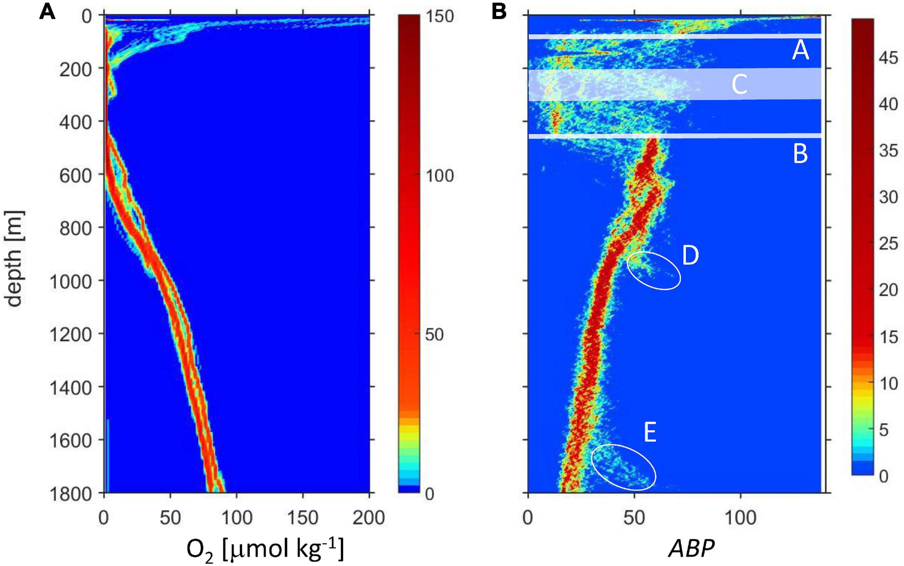
Figure 2. Depth profiles of oxygen (A) and ABP (B). The color indicates the number of data in a bin, for oxygen (4 m × 0.5 μmol kg^–1), for ABP (4 m × 0.7). In (B) are indicated: (A) Approximate depth of the upper oxycline. (B) Depth of the lower oxycline (lOx). (C) The depth of the intermediate oxygen maximum (iO₂) only encountered on some stations; ellipses (D,E): data from two stations on the shelf break.

We focused on the relationship between backscatter strength and oxygen concentration just below the lower oxycline (lOx) indicated in Figure 2 by line and also looked at the intermediate oxygen maximum band (iO₂) band C in Figure 2. Because the depths of iO₂ and lOx vary between stations, each profile had to be analyzed individually. For this, the depth of the lower oxycline (lOx) is defined by the first oxygen minimum recorded when the profiles were traced from the bottom up, around 500 m. This minimum oxygen concentration [O₂] is often not the lowest [O₂] recorded within the ODL.

Three main groups based on the depth profiles below the lower oxycline were identified (Figure 3A). The three color groups can be distinguished by the oxygen concentrations range at 150 m below the lOx, red: 0.7–2.0 μmol O₂ kg^–1; blue: 3–7 μmol O₂ kg^–1; black: 8–14 μmol O₂ kg^–1. The gray profiles in Figure 3A were difficult to classify. The regional distribution of these three groups indicates that the red profiles with the weakest depth gradient originate at the shelf break, blue stations are mainly found in the north and black stations in the south of the cruise region (Figure 1). We assume that the depth gradient below the ODL is determined by the balance of the vertical exchange coefficient of oxygen determined by hydrographic dynamics and the flux of organic particles that is supporting the oxygen consumption by organotrophic organisms.

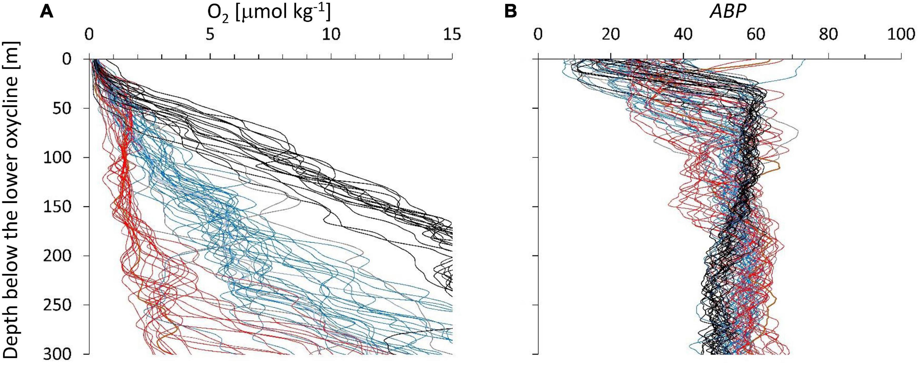
Figure 3. (A) The depth profiles of oxygen below the oxygen deficit layer showed different depth gradients. Depth on the ordinate is water depth minus lOx (around 500 m). (B) ABP vs. depth below lOx defined individually for each depth profile. We color-grouped the profiles according to their depth gradient from the strongest gradients (black) to the weakest gradients (red). Blue gradients are in-between and a few gray profiles were difficult to associate with a group.

The three color groups show an overall increase in ABP with distance below the ODL (Figure 3B) but the pattern is not very clear. The maximum ABP values (ABP_max) are reached at different depth distances below the ODL. The oxygen concentration at the maximum is within the suboxic range, which would classify it as part of the ODL layer according to our definition in the introduction. Near the lOx, the ABP profiles show a minimum value, but these minima are covering different values because the depth of the minimum ABP (ABP_min) did not exactly coincide with the depth we defined for lOx. However, a minimum ABP value was always reached close to lOx. Figure 4 shows the oxygen concentrations where ABP reached a minimum and where it reached a maximum below the lower oxycline. In Figure 4 the oxygen concentrations at ABP_min and ABP_max are again shown in a wider context.

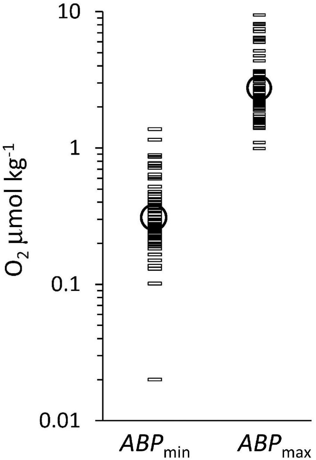
Figure 4. The oxygen concentration at ABP_min and at ABP_max, below lOx. Geometric means of the oxygen concentrations (circles) are at ABP_min: 0.31 μmol kg^–1 and at ABP_max: 2.7 μmol kg^–1. The difference between ABP_min and ABP_max, is significant (p < 0.05).

Here, the focus is on examining the relationship between [O₂] and ABP, looking at their depth profiles. One concern in the interpretation of ABP is the contribution of diurnally migrating populations. The long station 11 with 14 casts (see location in Figure 2) that included an iO₂ allowed evaluation of the effect of diurnal migrators on ABP profiles (Figure 5).

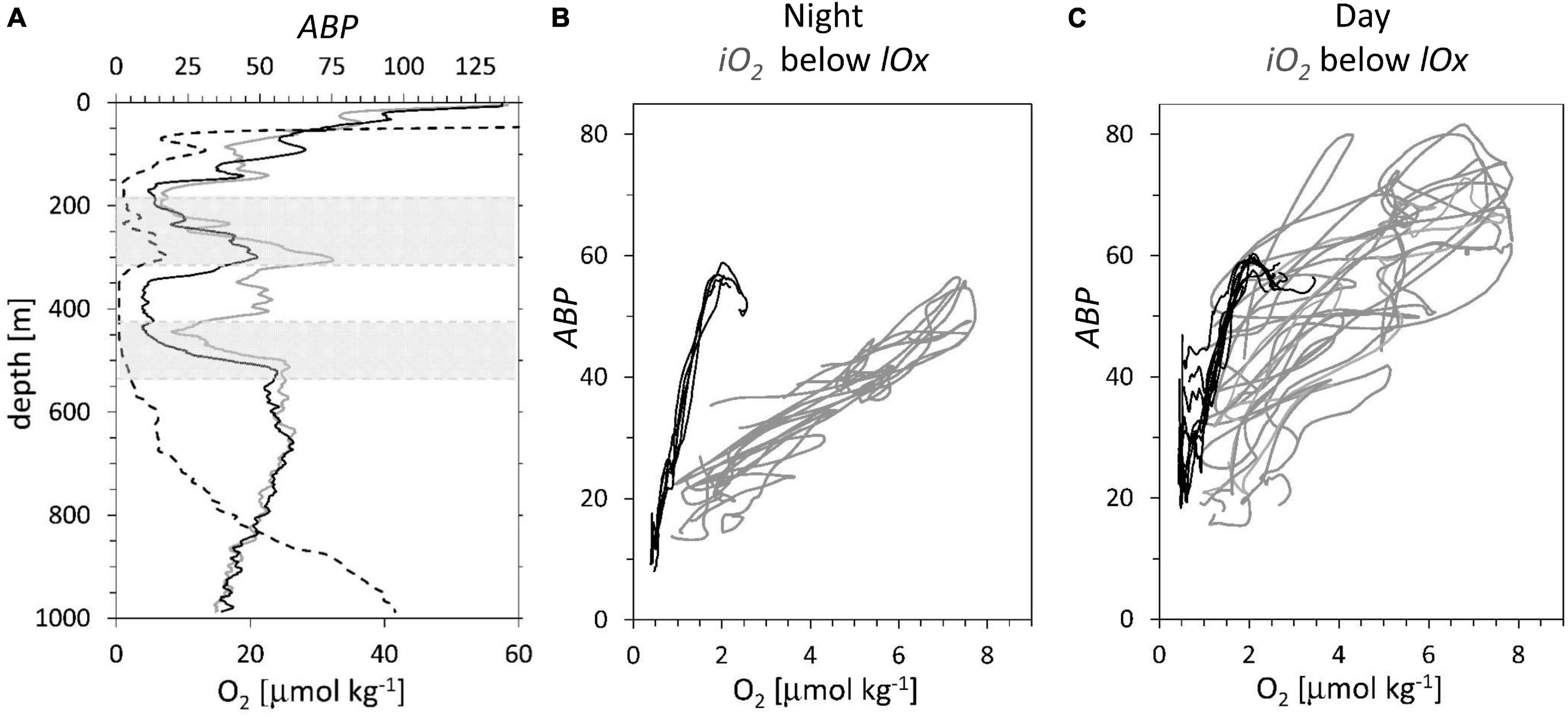
Figure 5. Data station 11, see Figure 1 for location, profiles taken at regular intervals during 53 h. (A) Two representative ABP profiles, at 12:20 solar day time (gray continuous line), at 24:00 (black line). Oxygen concentration (dotted line). Gray areas: depth ranges representing the iO₂ (185 to 315 m depth) and below the lOx (425 to 535 m depth). (B,C) ABP profiles vs. oxygen for the depth range of the iO₂ (gray lines) and below the lOx; (black lines). (B) 5 profiles taken at night, solar time 18:00 – 06:00. (C) 9 day profiles taken at solar time 06:00 – 18:00.

The differences between night (Figure 5B) and day (Figure 5C) profiles are due to diurnal vertical migration. During the night, the relationship between backscatter and [O₂] is linear (Figure 5B). The data below the lOx show a much steeper gradient than the data of the iO₂ with a peak at around 2.0 μmol kg^–1. This peak can be identified by the lower gray area in Figure 5A, representing the first ABP peak below the lOx. The 14 casts yielded an average in situ potential temperatures for the depth range of the iO₂: 12.1° +/−0.1°C and for the region below the lower oxycline: 8.13° +/−0.1°C. In Figure 5C, the day data below lOx show some additional backscatter due to migration at less than 1.0 μmol O₂ kg^–1, but the general pattern is largely maintained. In Figure 5C, the data of the iO₂ show in general higher backscatter values than in Figure 5B due to the presence of additional acoustic targets that migrated there during the day. Because the migrators do not position themselves according to the oxygen concentration, the linear relationship with [O₂] is largely lost. A comparison of black and gray lines in Figure 5C indicates that migrating ABP have little impact on the ABP vs. oxygen profiles below lOx, but in the intermediate oxygen maximum the migrating ABP obscures this relationship. Therefore, this work will focus on the depth region below lOx where a strong increase in ABP with an increase in oxygen concentration is observed.

The volume backscatter strength measured with ADCPs in the ocean is related to density gradients, quantity, shape, nature, and size of particles in the ocean (Foote and Stanton, 2000). Particles in the ocean are composed of organic and inorganic material, of abiotic and biotic, live and dead constituents. The use of ADCPs in all parts of the oceans to measure water movement by monitoring the movement of suspended particles is made possible because there are always suspended particles present. Only part of these particles is made up by organisms that we refer to here as acoustic backscatter population (ABP), for example species of copepods (e.g., Eucalanus inermis), Euphausia mucronata, even possibly of gelatinous organisms, foraminifera and fish larvae (e.g., Antezana, 1978; Ayon et al., 2008; Escribano et al., 2009; Wishner et al., 2013, 2018, 2020). Under conditions that are hostile to organisms, in the ODL or at great depth with low food supply, a minimum percentage of live organisms contributing to the volume backscatter is expected. To estimate the backscatter related to particles that we define as organisms, i.e., ABP, we subtracted a baseline (BB, equation 1), the background that is caused by unspecified live and dead particles. There is no fixed baseline that could be applied to one individual instrument because the baseline is not only defined by the electronic noise of the instrument but also by the acoustic characteristics of the echo particle population in situ and therefore by regional characteristics. Here for simplicity, we defined BB for the LADCP data using the lowest values recorded during the cruise (Supplementary Figures 2, 3), assuming that at all depths and regions the concentrations and acoustic properties of particles that were not organisms were similar. Bianchi et al. (2013) reviewed data from different cruises in different oceans, and they defined the lowest 10 percent of signals in each profile as a baseline to be subtracted from the ADCP profiles. This approach would not work for our data set because the lowest AVB values in a profile were mostly found within the ODL during the night when no migrating organisms increased the AVB signal (Supplementary Figure 2). During the day, the lowest AVB values could include migrating organisms, and therefore we used one single baseline value for all stations (Supplementary Figure 3). The BB value chosen for our data analysis may affect slightly our interpretation.

Figure 2 indicates a maximum ABP value (ABP_max) below the ODL, with a general monotonic decrease of ABP with greater depth. We propose that the organotrophic biomass represented by ABP is being maintained by organic particles sinking out of the ODL. The ABP depth profile below the ODL can be interpreted as resulting from two regimes of the response of organisms to environmental conditions: (1) between lOx and the ABP_max the organisms represented by ABP are oxygen limited, and (2) below ABP_max the organisms represented by ABP are limited by the availability of organic substrate. With depth below the ODL the particle flux is reduced by the consumption above and therefore this reduced particle flux is maintaining a decreasing ABP biomass with depth.

Below we focus our interpretation on two topics, the relation of ABP to the oxygen concentration and the relationship of depth-integrated ABP signals above and below the lower oxycline to show that the depth-integrated ABP below lOx is greater than above.

The Acoustic Backscatter Population vs. Oxygen Concentration

The data in Figure 6 include day and night profiles and all ABP groups show a very steep increase in ABP at very low [O₂] below the lOx. The data of different colors follow approximately the same pattern. The oxygen gradient at a low concentration range is sufficiently stable and spread over sufficient depth range (Figure 3A) to provide a pattern in Figure 6 with a nearly linear increase in ABP below 2 μmol O₂ kg^–1. These conditions are very different from the upper oxycline where the oxygen gradient is much steeper and the depth distribution of oxycline and zooplankton distribution is very variable in time and space (Bertrand et al., 2010). In Figure 6 some individual profiles show an increase in ABP at the lowest oxygen concentrations as observed in Figure 5C. In these cases, migrating backscatter populations are positioned at the lower oxycline during daylight modifying the expected pattern of an initial monotonic increase in backscatter population with an increase in oxygen. To model the ABP distribution with oxygen, we assumed that all ABP profiles in Figure 6 approach a similar maximum value below lOx, and at similar oxygen concentrations (Figure 4, ABP_max). If ABP is proportional to organismal biomass, then it can be assumed that this biomass is maintained by a similar flow of organic substrates that sink out of the ODL. The decrease in ABP below this maximum (Figure 2) should be due to a decreasing substrate flux with depth. In both oxygen gradients, within iO2 or below lOx (Figure 5B), the aerobic organisms will try to be as close as possible to the source of food, but are limited by the lack of oxygen when they approach zero [O₂]. The distribution of the aerobic organisms in the oxygen gradient within iO2 or below lOx will depend on their ability to metabolize organics at low [O₂]. ABP is not a rate, but it might be argued that the ABP concentration present at a certain oxygen concentration is related to the community metabolic rate, the sum of the metabolic rates of the different species at that oxygen concentration. In that case, the ABP vs. oxygen relation would follow a kinetic curve. Because ABP increases in a near linear manner with oxygen concentration (Figures 5B, 6) common asymptotic kinetics like Monod could not be applied to model ABP vs. oxygen concentration. We used the sigmoid Verhulst model (Eq. 2) for an empirical model relating ABP and the oxygen concentration [O₂] below the lOx in Figure 7:

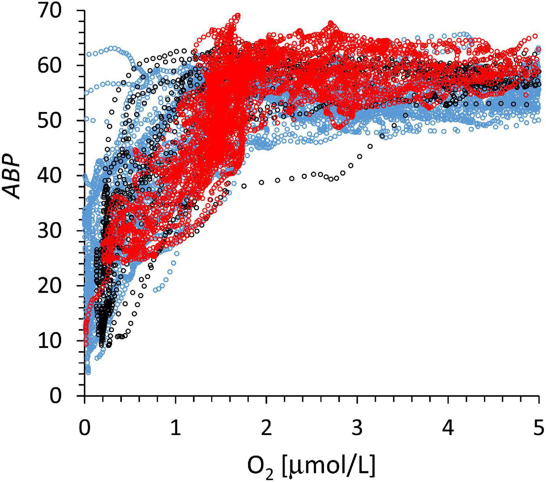
Figure 6. The baseline-corrected, ABP signal vs. oxygen between lOx (approximately 500 m). The depth at which oxygen concentration reaches 5 μmol kg^–1 ranges from 50 and 300 m below the lOx (Figure 3A). The line color code corresponds to that of Figure 3.

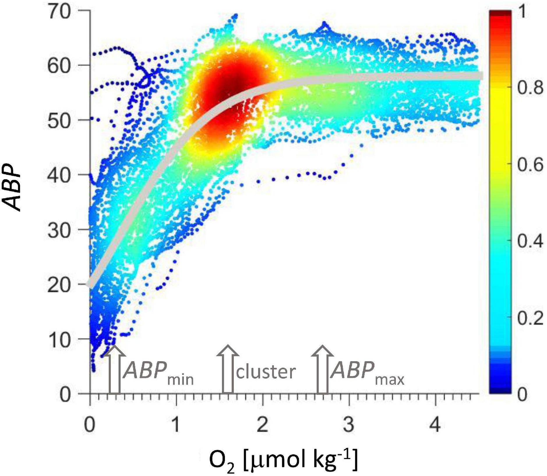
Figure 7. ABP vs. oxygen concentration. Colors indicate data density normalized to maximum data density. The gray line is the Verhulst model calculated according to Eq. 2.

The model was adjusted to the data in Figure 7 by minimizing the squared error (MatLab, routine lsqcurvefit) resulting in K = 58, x₀ = −54, r = 1.884 1/(μmol O₂ kg^–1), with r² = 0.72. Given the monotonous decrease in ABP with depth below ABP_max (Figure 2), the Verhulst model might be easily complemented with a function that describes this ABP decrease with depth if the model is to be expanded below the ABP_max to cover a greater depth range.

In Figure 7 data are color coded according to the normalized data density in a square of 0.17 μmol O₂ kg^–1 and 2.3 ABP, showing a clear maximum cluster at 1.6 μmol O₂ kg^–1 and 55 ABP. This maximum was used to normalize the color scale. This cluster signals the maximum occurrence of backscatter events at a certain oxygen concentration, indicating a condition that represents a sweet spot with sufficient oxygen concentration and sufficient proximity to the lower oxycline to maximize the gain from the organic particle flux leaving the ODL. The oxygen concentration at this cluster could serve as a reference for future net sampling efforts to consistently sample the organotrophic zooplankton maximum below the oxygen deficient layer. The oxygen concentration at the cluster maximum (Figure 7) is lower than at the ABP maximum below the lower oxycline (ABP_max).

An approximately linear increase of ABP is observed below 2 μmol O₂ kg^–1 (Figure 6) and at the latter oxygen concentration the Verhulst model calculates 95% of the maximum ABP value. Wishner et al. (2013) reported a secondary biomass peak maximum sampled with nets at that same low oxygen concentration below the oxygen minimum in the ETNP. The average oxygen concentration at the ABP_max was 2.7 μmol O₂ kg^–1 (Figure 4), this low oxygen concentration qualifies the organisms between lOx and ABP_max as microaerophils. Seibel and Deutsch (2020) suggested that organisms adapt their maximum physiological activity such that it matches their oxygen supply at the typical in situ oxygen partial pressure. They used a critical oxygen partial pressure (P_crit) as the partial pressure below which the organisms would not be able to sustain their basal metabolism at a certain temperature, and another point where partial pressure is sufficient to sustain maximum physiological activity (P_crit–max). The metabolic activity between both critical points is expected to be linearly related to the oxygen partial pressure. Under constant temperature and salinity, the molar concentration of oxygen would be proportional to partial pressure and a linear relation of metabolic activity and oxygen concentration would be expected. In the depth range represented by the data in Figure 7, the temperature and salinity changes are minor. Our data represent a proxy for biomass and not metabolic activity, but there are two similarities to the concept provided by Seibel (2011) and Seibel and Deutsch (2020), one is the near linear increase in biomass distribution with oxygen concentration and the ratio of O_2crit–max to O_2crit. The other similarity is that Seibel and Deutsch (2020) suggested that the lowest, basal physiological activity would be at 15 to 25 percent of the maximum activity and the lowest livable oxygen concentration would be proportionately reduced, suggesting a range of limiting oxygen concentration between four and seven. Their ratio is of similar magnitude as the ratio of oxygen concentrations at ABP_max (0.3 O₂ μmol kg^–1) to ABP_min (2.7 O₂ μmol kg^–1) (Figure 4). It should be emphasized that our data are biomass proxies and are not related to physiological rates, but maybe the in situ biomass distribution is proportional to the community metabolic rate that is supported by the local oxygen concentration. The different oxygen-depth gradients below the lOx (Figure 5) were stable for the duration of station 11 that lasted 53 h (Figure 5). These gradients are determined by regional hydrography in balance with microbial (Tiano et al., 2014; Canfield et al., 2019) and zooplankton aerobic respiration. Because these gradients were stable over a period longer than most organisms of an approximate size of 5 mm would need to position themselves within this gradient between ABP_min and ABP_max, the relation of ABP to oxygen should be determined by physiology.

The interpretation of the relation of oxygen concentration and biomass is complicated by changes in the taxonomic and age group composition of the biomass as observed by Wishner et al. (2018). Within the oxygen gradient between ABP_min and ABP_max the ABP community is probably not only composed of different taxa but also of different age groups with different physiological properties. However, the persistent relation of ABP vs. oxygen concentration (Figure 7) suggests that the ABP communities positioned themselves actively in this gradient of limiting oxygen concentrations. The oxygen concentration at ABP_max might be interpreted as the oxygen concentration where respiration saturates at the given temperature and substrate conditions, and that in the depth range between ABP_min and ABP_max the organisms balance oxygen limitation and access to food.

In Figure 5B both the data from station 11 within the iO₂ and below the lOx show linear slopes between ABP and the oxygen concentration during night-time, but the slope of the latter is four times steeper than the former. In this case, the slope ratio (lOx/iO₂) of four might be due to the community specific metabolic oxygen demand and respiratory efficiency (Deutsch et al., 2015). The temperature difference between 8.1°C (below lOx) and 12.1°C (iO₂) should produce an inverse tendency. Assuming a Q10 of 2, the respiration rate in the iO₂ could be 30% higher than below the lOx. This small change probably would not explain the strong change in the slope, a more likely explanation would be different taxonomic communities in both depth ranges.

The low oxygen concentration observed at the backscatter peak confirms the findings by Wishner et al. (2013, 2018) that “very small oxygen differences matter.” A mechanistic model of the ABP to oxygen relationship is not possible at this moment because the ABP community is probably composed of different species with different physiological properties at different parts of the oxygen gradient. One intriguing question is why a peak (ABP_max) is formed when the flux of organic substrate is sufficient to maintain large populations of ABP at greater depth.

The backscatter maximum below the lower oxycline (ABP_max) is significantly decreasing with a deeper lower oxycline (Figure 8: slope: −0.031, r²: 0.41, n: 72, p < 0.05). This change is relatively small since all pooled ABP_max values have a coefficient of variation of only 0.05 (Figure 8). One possible explanation for the relationship in Figure 8 would be that a deeper, lower oxycline implies more oligotrophic euphotic layer providing less organic particles to the bottom of the ODL. Depth-integrated chlorophyll values (0 to 100 m) showed no relation with ABP_max to confirm this hypothesis. The relationship of integrated chlorophyll to particle export and hence EPmax was probably obscured by horizontal advection and mesoscale activity (e.g., Bretagnon et al., 2018).

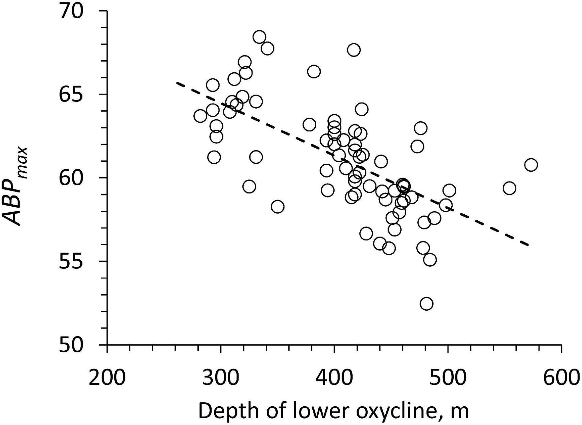
Figure 8. The ABP at the first peak below the lower oxycline (ABP_max) vs. the depth of the lower oxycline for each profile. The line shows the type 1 regression.

Depth-Integrated Acoustic Backscatter Populations

To evaluate the ecological weight of the echo population below the ODL we compared the depth integrals of the echo populations compared below and above the lower oxycline, lOx. The integrals are defined in Equations 3 and 4:

Echo population above the lower oxycline:

Echo population below the bottom oxycline:

Zb is the depth of lOx, ABP_z is the echo population at depth z, IABP_up is the integrated echo population above the lower oxycline and IABP_down from the oxycline to 1000 m below. We used a fixed distance of 1000 m below the lower oxycline to delimit the integral to a depth range that would make integrals with different lOx more comparable. Because the relation of ABP and population biomass is not known and probably variable, particularly at different depths and in different ecological settings, our ratio of depth-integrated ABP can only provide a rough qualitative comparison. However, a fixed depth interval below the lOx should include similar ABP organismal composition facilitating comparison of profiles. The ABP ratio (IABP_down / IABP_up) average is 2.36 (S.D.: 0.71), suggesting that the backscatter population below the oxygen deficit layer is significantly greater than the population above, reaching from lOx to the surface. Because the limit was set at lOx, the ratio is not significantly affected by the migrating population, that is generally staying above the lOx (see black lines at the lowest O₂ concentrations in Figure 5C). Organotrophic biomass standing stock is sustained mainly by the availability of organic carbon; in the case of organisms below the lOx this would be the flux of organic particles sinking out of the ODL. Therefore, the high ABP ratio suggests a high carbon export flux from the euphotic layer, a carbon flux that is largely conserved within the ODL depth range because of limited metabolic activity of organotrophic organisms. We propose that the supply rate of organic particles available for nourishment of the backscatter populations below and above the lower oxycline largely determines the ABP ratio. However, our interpretation does not consider other obvious ecological controls of the ABP biomass such as limitations of population growth by lack of oxygen or the control by predators.

The sum of IABP_down and IABP_up may be interpreted as an indicator of productivity at the surface that is sustaining the depth integrated echo population at the station. A type 2 linear regression of the data in Figure 9 yielded: slope: −1.0024E-4, st.dev. 1.33E-5; y-intercept: 8.15, st.dev. 0.755; n: 72; Pearson correlation coefficient: 0.672, p < 0.05. We found no statistical relationship between depth-integrated chlorophyll (0 to 100 m) and the sum of IABP_down and IABP_up to support a functional relation between both. If IABP_down and IABP_up is related to the trophic state then it is surprising that in more oligotrophic conditions a greater portion of the population resided below the ODL, because under those conditions a lower particle transfer efficiency to deep waters would be expected.

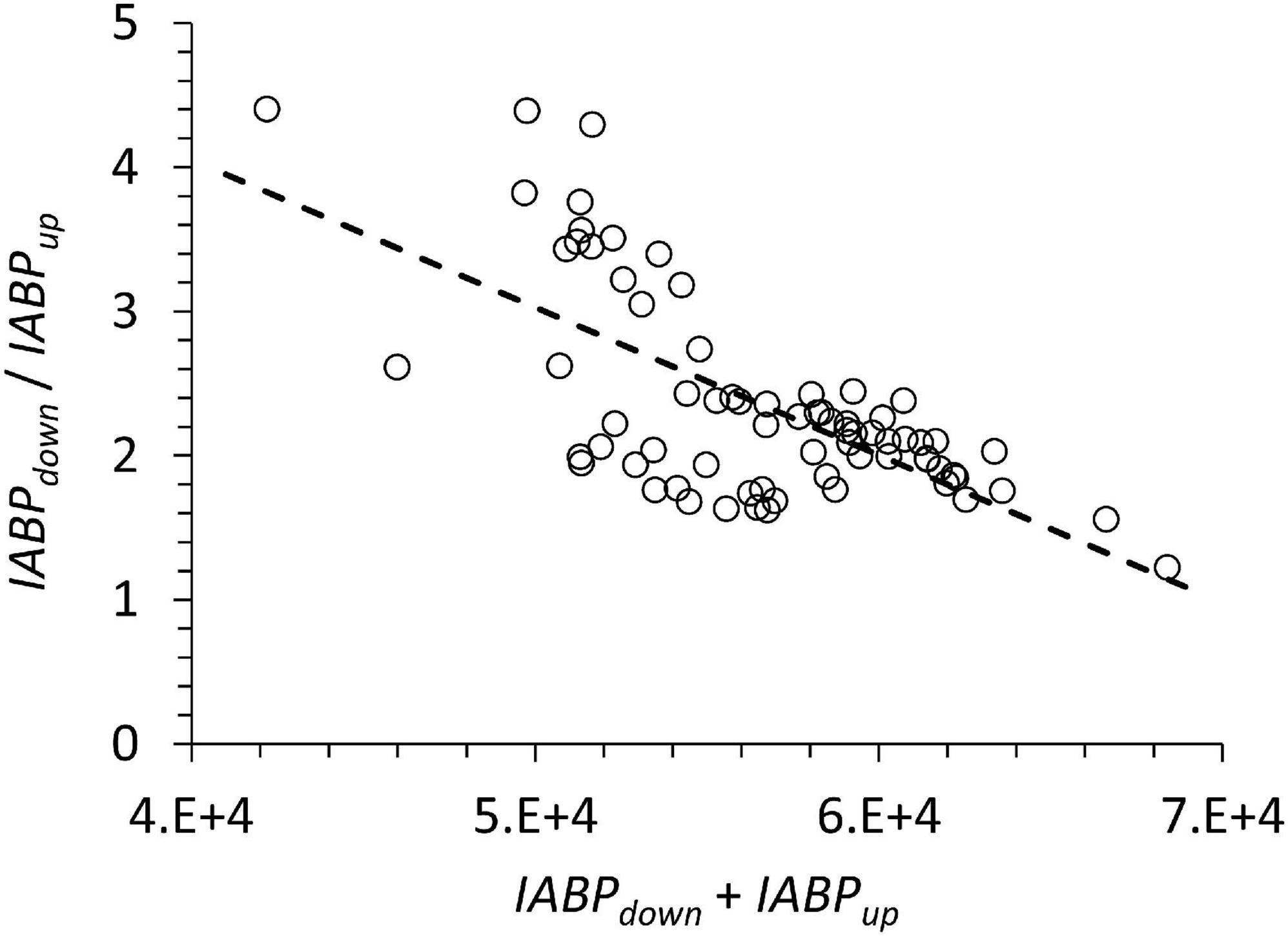
Figure 9. The ratio of IABP_down / IABP_up is behaving inversely to the sum of IABP_down and IABP_up.

Any interpretation of the ratio IABP_down / IABP_up is only valid if the average ratio of biomass to acoustic backscatter is independent of depth, where the populations above and below lO show similar acoustic properties at 300 kHz. One limitation of the volume backscatter at a certain acoustic frequency is that the backscatter is not strictly limited to the particles or organisms with dimensions similar to the acoustic wavelength but can include organisms of different sizes (Foote and Stanton, 2000) that might represent different trophic levels.

For a larger ecological interpretation, for example vertical carbon transport, it would help to include other trophic levels and size classes. Wishner et al. (2013) showed differences in relative biomass size distribution between 0.2 to 5 mm and >5 mm in two different stations in the oxygen minimum region of the ETNP during day and night. One notable pattern was that at the lower oxycline the size classes >5 mm and 2–5 mm dominated, whereas within the oxygen minimum mostly the 1–2 mm biomass class dominated. The 2 to >5 mm size classes are closer to the acoustic wavelength, which suggests that the ABP to biomass ratio was greater below the oxygen minimum. The value of the ratio also depends on the value of the baseline chosen (equation 1). Here we have chosen 90 (Supplementary Figures 2, 3): a lower baseline value would decrease the ratio. In Figure 9 the data of the sum of IABP_down and IABP_up have a coefficient of variation of 0.082 not that much higher than the coefficient of variation of ABP_max (Figure 8), which suggests little difference in the trophic state at the different stations included in this study.

Considering that diurnal vertical migration reached to the bottom of the ODL (Figure 4), we looked at its possible effect on the depth-integrated backscatter populations. We expected little diurnal variation in the ABP_max and the sum of IABP_down and IABP_up values because Figures 8, 9 showed a low coefficient of variation of less than 10% for all the data. We evaluated if the sum of IABP_down and IABP_up was subject to diurnal changes. The diurnal cycles in Figure 10 of the ratio of IABP_down / IABP_up showed a minimum at noon and the sum of IABP_down and IABP_up showed a maximum.

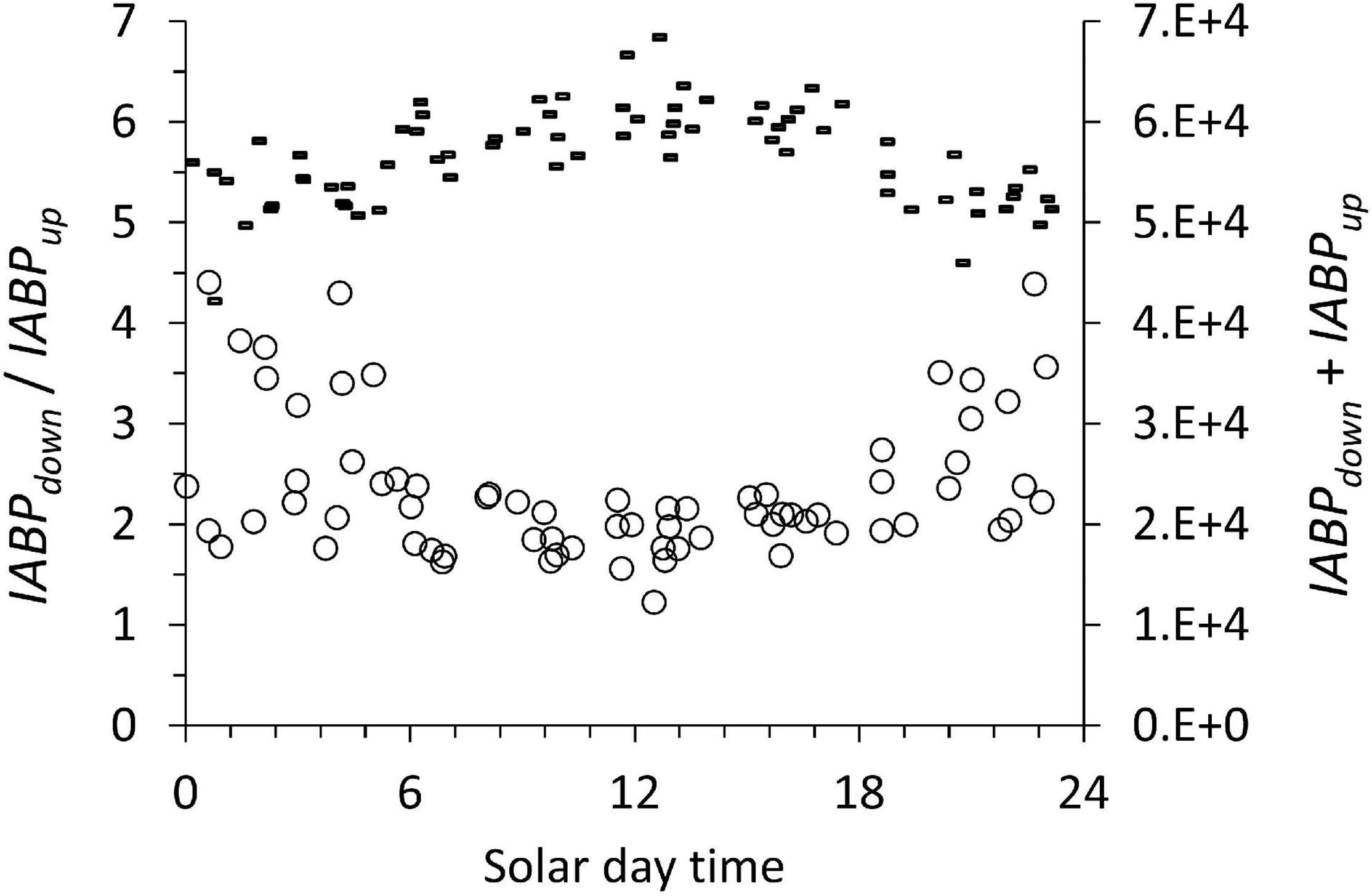
Figure 10. The ratio of IABP_down / IABP_up (circles, left ordinate) and the sum of IABP_down and IABP_up (dashes right ordinate) during the diurnal cycle. The data include all the profiles at all stations considered in this work.

The diurnal pattern (Figure 10) can be traced to the integrated IABP_up of the upper layer that shows a maximum at noon (Figure 11, circles). The depth-integrated echo population below the ODL (IABP_down) did not change significantly during the day with a coefficient of variation of 0.07 (Figure 10, dashes). The relatively low variance of IABP_down is surprising considering that the data from stations on the shelf edge or outside the continental shelf are included here (Figure 2).

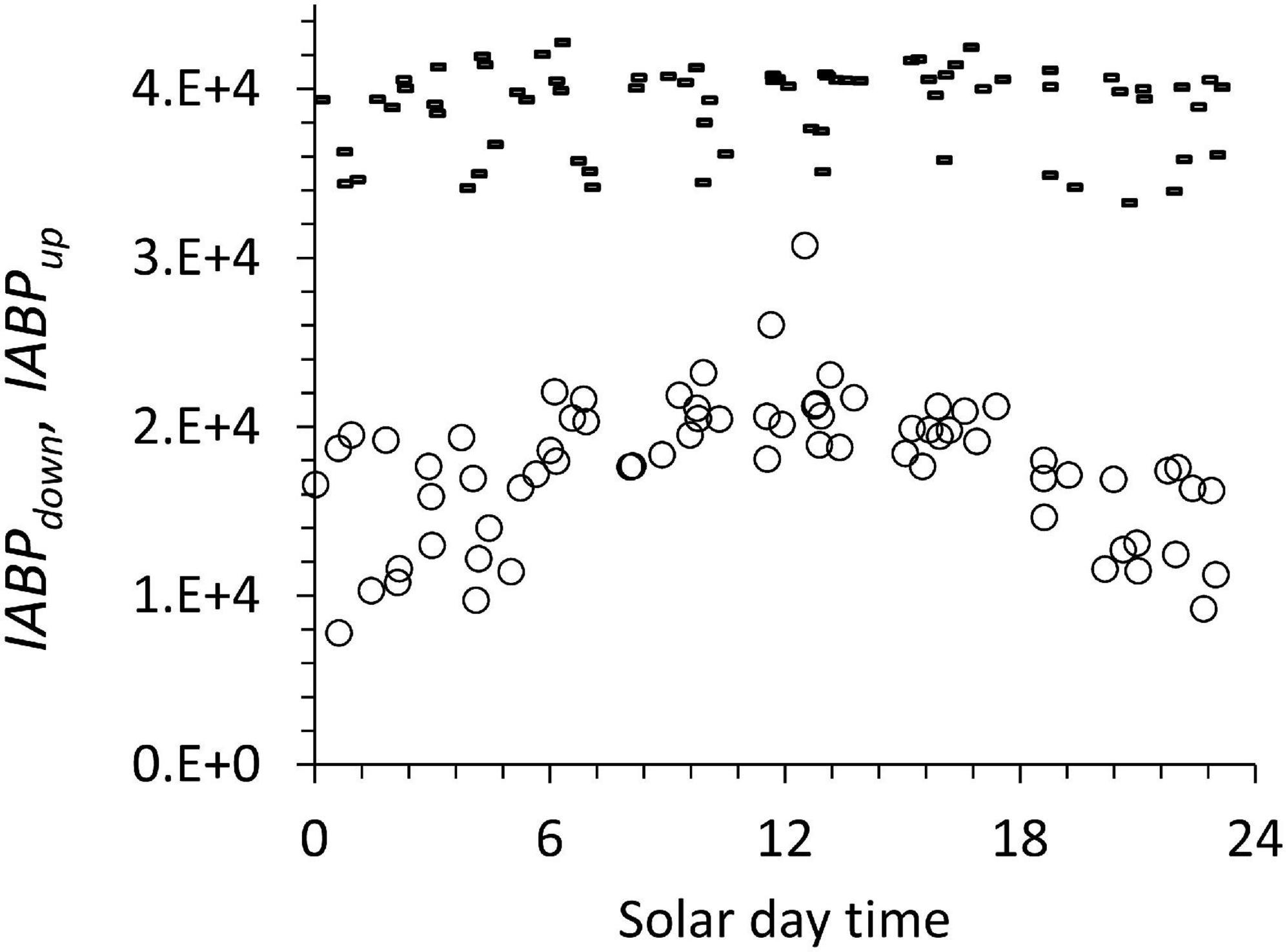
Figure 11. IABP_down (dashes) and IABP_up (circles) during the diurnal cycle. These data include all the profiles from the different stations considered in this work.

One likely source of the diurnal change in IABP_up is that at night a significant portion of the IABP_up population is located in the top 5 m of the water column that the LADCP did not measure. In our data treatment, we extrapolated the value at 6 m depth to the surface (see Supplement). This extrapolation might have underestimated the true echo population during the night that was congregated less than 6 m from the surface. Following this argument, then the noon values of the IABP_down to IABP_up ratio would be the correct data. These noon values still support the conclusion that IABP_down is significantly bigger than IABP_up.

We are aware that the ABP can only be interpreted as organismal biomass of a certain size range, and depends on form, orientation to the sound source, and material acoustic properties. We expect that these properties allow for a significant range of biomass to ABP ratios [see “Introduction” in Postel et al. (2007)]. For a wider ecological interpretation, metabolic rates and the concentrations of higher trophic levels are missing, e.g., the predators of the organisms representing ABP. The steady state standing stock of a population is determined by the balance of the rates of growth and loss, mainly by predation. However, our interpretation that the high ratio of the IABP_down to IABP_up is made possible by the efficient transport through the ODL and high sedimentation of particulate organics produced in the euphotic zone, partly resulting of the low depredation in the ODL, we consider this to be the simplest and most straightforward explanation. The efficient transport of organics through the mesopelagic layer has been documented by several authors. Martin et al. (1987) measured a greater remineralization length coefficient at a station off Peru interpreting this as typical for a region with ODL. Wishner et al. (1990) observed the accumulation of high biomass sedimented on top a seamount within the ETNP oxygen minimum. Cavan et al. (2017) discussed the possible reasons why the transport of organics through the ODL would be less attenuated than in the water columns with higher oxygen concentrations. They concluded for the ETNP oxygen minimum that the vertical particle flux was less reduced with depth because in the ODL the zooplankton presence and activity was decreased, resulting in less coprorhexy, i.e., the fragmentation of organic particle. Keil et al. (2016) also observed less flux attenuation within the ODL in the Arabian Sea, similar to Cavan et al. (2017) they attributed it to changes in zooplankton activity and sinking speed of organics, in addition to microbial activity in the upper part of the ODL. Off Peru but only outside the continental shelf, Dale et al. (2015) also found indications of a reduced attenuation of the organic particle flux through the ODL.

Conclusion

The LADCP volume backscatter profiles showed persistent, non-migrating populations at intermediate oxygen maxima (iO₂) within the oxygen deficient layer (ODL) and below the ODL. In both cases, the acoustic backscatter population (ABP) maintained a linear relation over very few O₂ μmol kg^–1 as expected for microaerophils or hypoxic species in ODL regions. The ABP in the intermediate oxygen maximum iO₂ had lesser affinity to oxygen than ABP below the lOx but both showed population maxima at only a few μmoles kg^–1. We have no information on metabolic rates, but we propose that these two ecological niches, iO₂ and below the lOx, are populated by different hypoxic species adapted to express their maximum metabolic rates at the oxygen concentrations and temperatures found at the respective backscatter population maxima: in the iO₂, at 5.0 μmol kg^–1; and below lOx, at 2.7 O₂ μmol kg^–1. In both niches, the accumulation of the population was made possible by a constant supply of sinking organic particles. Although these organisms reached their maxima at these very low oxygen concentrations, it is unclear if they can reproduce under these conditions. The interpretation of ABP is complicated by the fact that the backscatter signal is related to the size and shape spectrum of the organisms. A closer ecological interpretation would have to consider that the population is probably composed of different organisms and/or different life stages of the same organism. Wishner et al. (2020) used sophisticated net sampling methods to obtain samples within the low oxygen concentration gradient below the ODL, and they showed that the concentration gradient can also be a gradient in taxonomic and life-stages composition.

We estimated the depth-integrated backscatter population above and below the lower oxycline and found over a distance of 1200 km parallel to the coast a constant pattern of greater depth-integrated populations below the bottom of the ODL than above. These results suggest that a considerable proportion of the surface primary production is transported below the ODL in the open ocean, which is made possible because the organic particle flux is little attenuated during sinking through the ODL. Several authors documented the efficient transport of organics through the mesopelagic ODL which implies that more particulate organics settle out of the ODL layer than would be expected at the same depth in an oxygenated water column, supporting our hypothesis that the accumulated acoustic backscatter population is maintained by the particulate organics raining out of the ODL.

Data Availability Statement

The original contributions presented in the study are included in the article/Supplementary Material, further inquiries can be directed to the corresponding author/s.

Author Contributions

GE, BD, JS, JG, KM-V, and OV performed data taking. AP, GE, JO, VG, and HM performed the data processing. HM, GE, VG, and AP wrote and edited the manuscript. All authors contributed to the article and approved the submitted version.

Funding

This work was supported by the AMOP (“Activity of research dedicated to the Minimum of Oxygen in the eastern Pacific”) project, thanks to CNRS-INSU, IRD and SYSCO2/LEGOS team funding. The French funding included the participation of HM in the cruise and in a post-cruise reunion for data analysis, in particular thanks to PICS MESOX (CNRS). JO generously dedicated spare time to the analysis of the LADCP data. BD acknowledges support from ANID (Concurso de Fortalecimiento al Desarrollo Científico de Centros Regionales 2020-R20F0008-CEAZA and grant 1190276).

Conflict of Interest

The authors declare that the research was conducted in the absence of any commercial or financial relationships that could be construed as a potential conflict of interest.

Publisher’s Note

All claims expressed in this article are solely those of the authors and do not necessarily represent those of their affiliated organizations, or those of the publisher, the editors and the reviewers. Any product that may be evaluated in this article, or claim that may be made by its manufacturer, is not guaranteed or endorsed by the publisher.

Acknowledgments

We would like to thank the crew of the French R/V Atalante, and Anne Royer, Emmanuel de Saint Léger and Olivier Depretz De Gesincourt from French Technical Division (INSU/CNRS) for general logistics support. We also like to thank Miriam Soto (IRD-Peru) and Cécile Henry (French Embassy, Peru) for general administrative support.

Supplementary Material

The Supplementary Material for this article can be found online at: https://www.frontiersin.org/articles/10.3389/fmars.2021.723056/full#supplementary-material

Footnotes

1. ^ http://met.igp.gob.pe/datos/icen.txt

References

Antezana, T. (1978). Distribution Of Euphausiids In The Chile-Peru Current With Particular Reference To The Endemic E. Mucronata And The Oxygen Minimum Layer. Ph.D. thesis. La Jolla, CA: Scripps Institution of Oceanography.
Ayon, P., Criales-Hernandez, M. I., Schwamborn, R., and Hirche, H. J. (2008). Zooplankton research off Peru: a review. Prog. Oceanogr. 79, 238–255.
Bertrand, A., Ballo’n, M., and Chaigneau, A. (2010). Acoustic observation of living organisms reveals the upper limit of the oxygen minimum zone. PLoS One 5:e10330. doi: 10.1371/journal.pone.0010330
Bianchi, D., Galbraith, E. D., Carozza, D. A., Mislan, K. A. S., and Stock, C. A. (2013). Intensification of open-ocean oxygen depletion by vertically migrating animals. Nat. Geosci. 6, 545–548. doi: 10.1038/NGEO1837
Breitburg, D., Levin, L. A., Oschlies, A., Grégoire, M., Chavez, F. P., Conley, D. J., et al. (2018). Declining oxygen in the global ocean and coastal waters. Science 359:eaam7240. doi: 10.1126/science.aam7240
Bretagnon, M., Paulmier, A., Garçon, V., Dewitte, B., Illig, S., Leblond, N., et al. (2018). Modulation of the vertical particle transfer efficiency in the Oxygen Minimum Zone off Peru. Biogeoscience 15, 5093–5111. doi: 10.5194/bg-15-5093-2018
Brewer, P. G., and Hofmann, A. F. (2014). A plea for temperature in descriptions of the oceanic oxygen status. Oceanography 27, 160–167. doi: 10.5670/oceanog.2014.19
Canfield, D. E., and Thamdrup, B. (2009). Towards a consistent classification scheme for geochemical environments, or, why we wish the term ‘suboxic’ would go away. Geobiology 7, 385–392.
Canfield, D. E., Kraft, B., Löscher, C. R., Boyle, R. A., Thamdrup, B., and Stewart, F. J. (2019). The regulation of oxygen to low concentrations in marine oxygen-minimum zones. J. Mar. Res. 77, 297–324. doi: 10.1357/002224019828410548
Cavan, E. L., Trimmer, M., Shelley, F., and Sanders, R. (2017). Remineralization of particulate organic carbon in an ocean oxygen minimum zone. Nat. Commun. 8:14847. doi: 10.1038/ncomms14847
Chavez, F. P., Bertrand, A., Guevara-Carraso, R., and Csirke, J. (2008). The northern humboldt current system: brief history, present status and a view towards the future. Prog. Oceanogr. 79, 95–105.
Dale, A. W., Sommer, S., Lomnitz, U., Montes, I., Treude, T., Liebetrau, V., et al. (2015). Organic carbon production, mineralisation and preservation on the Peruvian margin. Biogeosciences 12, 1537–1559.
Deutsch, C., Ferrel, A., Seibel, B., Pörtner, H. O., and Huey, R. B. (2015). Climate change tightens a metabolic constraint on marine habitats. Science 348:1132. doi: 10.1126/science.aaa1605
Escribano, R., Hidalgo, P., and Krautz, C. (2009). Zooplankton associated with the oxygen minimum zone system in the northern upwelling region of Chile during March 2000. Deep Sea Res. II 56, 1083–1094. doi: 10.1016/j.dsr2.2008.09.009
Foote, G., and Stanton, T. K. (2000). “Acoustical methods,” in ICES Zooplankton Methodology Manual, eds H.-R. Skjoldal, J. Lenz, M. Huntley, P. Wiebe, and R. Harris (San Diego, CA: Academic Press), 223–253.
Fuenzalida, R., Schneider, W., Garcés-Vargas, J., Bravo, L., and Lange, C. (2009). Vertical and horizontal extension of the oxygen minimum zone in the eastern South Pacific Ocean. Deep Sea Res. Part II 56, 992–1003. doi: 10.1016/j.dsr2.2008.11.001
Gallo, N. D., and Levin, L. A. (2016). Fish ecology and evolution in the world’s oxygen minimum zones and implications of ocean deoxygenation. Adv. Mar. Biol. 1, 1–81. doi: 10.1016/bs.amb.2016.04.001
Garcia-Robledo, E., Padilla, C. C., Aldunate, M., Stewart, F. J., Ulloa, O., Paulmier, A., et al. (2017). Cryptic oxygen cycling in anoxic marine zones. Proc. Natl. Acad. Sci. U.S.A. 114, 8319–8324. doi: 10.1073/pnas.1619844114
Garcia-Robledo, E., Paulmier, A., Borisov, S., and Revbesch, N. (2021). Sampling in low oxygen aquatic environments: the deviation from anoxic conditions. Limnol. Oceanogr. doi: 10.1002/lom3.10457
Hofmann, A. F., Peltzer, E. T., and Brewer, P. G. (2013). Kinetic bottlenecks to respiratory exchange rates in the deep-sea – part 1: oxygen. Biogeosciences 10, 5049–5060. doi: 10.5194/bg-10-5049-2013
Keil, R. G., Neibauer, J., Biladeau, C., van der Elst, K., and Devol, A. H. A. (2016). Multiproxy approach to understanding the ‘enhanced’ flux of organic matter through the oxygen deficient waters of the Arabian Sea. Biogeosciences 13, 2077–2092.
Kiko, R., and Hauss, H. (2019). On the estimation of zooplankton-mediated active fluxes in Oxygen Minimum Zone regions. Front. Mar. Sci. 6:741. doi: 10.3389/fmars.2019.00741
L’Heureux, M., Takahashi, K., Watkins, A., Barnston, A., Becker, E., Di Liberto, T., et al. (2017). Observing and predicting the 2015–2016 El Niño. Bull. Am. Meteor. Soc. 98, 1363–1382. doi: 10.1175/BAMS-D-16-0009.1
Laufkötter, C., John, J. G., Stock, C. A., and Dunne, J. P. (2017). Temperature and oxygen dependence of the remineralization of organic matter, Global Biogeochem. Cycles 31, 1038–1050. doi: 10.1002/2017GB005643
Margolskee, A., Frenzel, H., Emerson, S., and Deutsch, C. (2019). Ventilation pathways for the North Pacific oxygen deficient zone. Glob. Biogeochem. Cycles 33, 875–890. doi: 10.1029/2018GB006149
Martin, J. H., Knauer, G. A., Karl, D. M., and Broenkow, W. W. (1987). VERTEX: carbon cycling in the northeast Pacific. Deep Sea Res. A Oceanogr. Res. Pap. 34, 267–285.
Mullison, J. (2017). “Backscatter estimation using broadband acoustic doppler current profilers- updated,” in Proceedings of the ASCE Hydraulic Measurements & Experimental Methods Conference, July 9-12, 2017, Durham, NH.
Paulmier, A., and Ruiz-Pino, D. (2009). Oxygen minimum zones (OMZs) in the modern ocean. Prog. Oceanogr. 80, 113–128. doi: 10.1016/j.pocean.2008.08.001
Pauly, D. (2021). The gill-oxygen limitation theory (GOLT) and its critics. Sci. Adv. 7:eabc6050. doi: 10.1126/sciadv.abc6050
Pennington, J. T., Mahoney, K. L., Kuwahara, V. S., Kolber, D. D., Calnies, R., and Chavez, F. P. (2006). Primary production in the eastern tropical Pacific: a review. Prog. Oceanogr. 69, 285–317. doi: 10.1016/j.pocean.2006.03.012
Postel, L., da Silva, A. J., Mohrholz, V., and Lass, H. U. (2007). Zooplankton biomass variability off Angola and Namibia investigated by a lowered ADCP and net sampling. J. Mar. Syst. 68, 143–166. doi: 10.1016/j.jmarsys.2006.11.005
Seibel, B. (2011). Critical oxygen levels and metabolic suppression in oceanic oxygen minimum zones. J. Exp. Biol. 214, 326–336. doi: 10.1242/jeb.049171
Seibel, B., and Deutsch, C. (2020). Oxygen supply capacity in animals evolves to meet maximum demand at the current oxygen partial pressure regardless of size or temperature. J. Exp. Biol. 223:jeb210492. doi: 10.1242/jeb.210492
Tiano, L., Garcia-Robledo, E., Dalsgaard, T., Devol, A. H., Ward, B. B., Ulloa, O., et al. (2014). Oxygen distribution and aerobic respiration in the north and south eastern tropical Pacific oxygen minimum zones. Deep Sea Res. Part I 94, 173–183. doi: 10.1016/j.dsr.2014.10.001
Vaquer-Sunyer, R., and Duarte, C. M. (2011). Temperature effects on oxygen thresholds for hypoxia in marine benthic organisms. Glob. Change Biol. 17, 1788–1797.
Wishner, K. F., Levin, L., Gowing, M., and Mullineaux, L. (1990). Involvement of the oxygen minimum in benthiczonation on a deep seamount. Nature 346, 57–59.
Wishner, K. F., Outram, D. M., Seibel, B. A., Roman, C., Daly, K. L., and Williams, R. L. (2013). Zooplankton in the eastern tropical north Pacific: boundary effects of oxygen minimum zone expansion. Deep Sea Res. 79, 122–140. doi: 10.1016/j.dsr.2013.05.012
Wishner, K. F., Seibel, B. A., Roman, C., Deutsch, C., Outram, D., Shaw, C. T., et al. (2018). Ocean deoxygenation and zooplankton: very small oxygen differences matter. Sci. Adv. 4:eaau5180. doi: 10.1126/sciadv.aau5180
Keywords: microaerobic zooplankton, lowered ADCP, oxygen minimum zone (OMZ), biomass below OMZ, Eastern Tropical South Pacific
Citation: Paulmier A, Eldin G, Ochoa J, Dewitte B, Sudre J, Garçon V, Grelet J, Mosquera-Vásquez K, Vergara O and Maske H (2021) High-Sustained Concentrations of Organisms at Very low Oxygen Concentration Indicated by Acoustic Profiles in the Oxygen Deficit Region Off Peru. Front. Mar. Sci. 8:723056. doi: 10.3389/fmars.2021.723056
Received: 09 June 2021; Accepted: 06 September 2021;
Published: 28 September 2021.
Edited by:
Laura Anne Bristow, University of Southern Denmark, DenmarkReviewed by:
Karen Wishner, The University of Rhode Island, United StatesHelena Hauss, GEOMAR Helmholtz Centre for Ocean Research Kiel, Germany
Copyright © 2021 Paulmier, Eldin, Ochoa, Dewitte, Sudre, Garçon, Grelet, Mosquera-Vásquez, Vergara and Maske. This is an open-access article distributed under the terms of the Creative Commons Attribution License (CC BY). The use, distribution or reproduction in other forums is permitted, provided the original author(s) and the copyright owner(s) are credited and that the original publication in this journal is cited, in accordance with accepted academic practice. No use, distribution or reproduction is permitted which does not comply with these terms.
*Correspondence: Helmut Maske, hmaske@cicese.mx