Deep Machine Learning for Forecasting Daily Potential Evapotranspiration in Arid Regions, Case: Atacama Desert Header

Abstract

Accurately estimating and forecasting evapotranspiration is one of the most important tasks to strengthen water resource management, especially in desert areas such as La Yarada, Tacna, Peru, a region located at the head of the Atacama Desert. In this study, we used temperature, humidity, wind speed, air pressure, and solar radiation from a local weather station to forecast potential evapotranspiration (ETo) using machine learning. The Feedforward Neural Network (Multi-Layered Perceptron) algorithm for prediction was used under two approaches: “direct” and “indirect”. In the first one, the ETo is predicted based on historical records, and the second one predicts the climate variables upon which the ETo calculation depends, for which the Penman-Monteith, Hargreaves-Samani, Ritchie, and Turc equations were used. The results were evaluated using statistical criteria to calculate errors, showing remarkable precision, predicting up to 300 days of ETo. Comparing the performance of the approaches and the machine learning used, the results obtained indicate that, despite the similar performance of the two proposed approaches, the indirect approach provides better ETo forecasting capabilities for longer time intervals than the direct approach, whose values of the corresponding metrics are MAE = 0.033, MSE = 0.002, RMSE = 0.043 and RAE = 0.016.

1. Introduction

Nowadays, great efforts are made to achieve an efficient use of water in economic activities, especially in agriculture; activity that registers the highest water consumption in the world. Accurate prediction of vegetation water consumption is important in the fields of hydrology and irrigation engineering [1]. Evapotranspiration (ET) is one of the most important components of the hydrological cycle and its accurate estimation is very important for the hydrological water balance, design, and management of irrigation systems, crop yield, and water resources planning [2,3,4,5]. Likewise, it plays an essential role in simulating the hydrological effects of climate change [6].

Various methods have been developed over time to estimate potential evapotranspiration (ETo) from weather data. These methods vary in complexity from models that require only basic information, such as the maximum and minimum air temperatures, to complex models that estimate ETo through energy balance models, such as the Penman-Monteith method [7].

To date, there have been attempts to estimate and predict ETo more accurately. Some of them involve numerical and statistical approaches that attempt to accurately simulate the random nature of climate variables [8]. In parallel, artificial intelligence techniques have been developed with the use of tools based on statistical learning theory, such as artificial neural networks [9,10,11,12].

Artificial neural networks (ANNs) are a mathematical approach to the functioning of the brain that can be schematically represented for better understanding [13]. The use of ANNs is widespread, although conventional machine learning (ML) methods, including ANN, principal component analysis (PCA), support vector machines (SVM), and regression analysis, among others, have been successfully used for decades. Recent advances in deep learning have aroused special interest in academia by the intelligent monitoring of various natural and artificial processes [14]. The reason for selecting the Multilayer Perceptron in this research was its ease of implementation. MLP is also known for providing high-quality models while keeping the learning time relatively low compared to more complex methods [15]. Likewise, time series forecasting is becoming one of the most important branches of big data analysis [16]. Hydrology is not unrelated to this and especially ETo forecasting, which is used in crop irrigation scheduling.

The reference evapotranspiration (ETr) is usually computed in advance to obtain the actual evapotranspiration (ETa). For the ETo estimation, artificial intelligence techniques, specifically ML, are suitable methodologies due to their excellent computational efficiency and less dependence on data [17].

In Peru, similar works have been developed [12,18], but in high Andean basins that also use meteorological information; however, other approaches, such as the one addressed by this research, have not been considered. In addition, in the Tacna Region, there are no similar studies.

There are proposals for comparing the calculation of ETr with different methods. For instance, Yang [19] makes a detailed comparison of methods based on temperature and radiation using computational techniques implemented in MATLAB, with significant results. Nowadays, ML is becoming a widely used tool in hydrology [20]. Research proposals using data science are increasing in the calculation of ETr and especially in the validation of the precision of various classical and some recent methods [21]. Specifically, deep learning using neural networks has become a very powerful and interesting alternative for the prediction of climate variables based on temperature [9].

This study aims to test the efficiency of two approaches (direct and indirect) to predict daily ETo in an arid region located in southern Peru, using machine learning with daily climate information from an automatic recording station scheduled to 30 min. The algorithm used corresponds to an MLP (Multi-Layer Perceptron) neural network architecture, to determine the suitability of the proposed forecasting schemes, using the hyperbolic tangent as an activation method that delivers transformed values between −1 and 1. For the forecasting effort, we considered ETo values derived from the equations of Penman-Monteith [7], Hargreaves [22], Ritchie [23], and Turc [24].

The research goal of this study is to devise a predictive model to calculate the evotranspiration of our study zone and compare this with other methods. The model may be well extended to other arid zones. In this direction, this study attempts to answer the following research questions:

RQ1: Can time series data be adequately transformed into data from supervised problems to apply to neural network models?

RQ2: Can an acceptable accuracy of evapotranspiration prediction be obtained using multilayer perceptron?

RQ3: Can a deep learning model perform better than calculation applying the Penman-Monteith, Hargreaves-Simoni, Ritchie, and Turc equations in arid zones?

Our main hypothesis is that using deep learning models we can obtain a high degree of precision in evapotranspiration prediction in the arid zone of Tacna.

2. Theoretical Foundations of Evapotranspiration

Several authors [22,23,24,25] have studied evapotranspiration dynamics; in this sense, the present study uses these definitions and formulations to be able to compare the calculations of evapotranspiration with the prediction based on neural networks. Next, we will make a brief description of the formulations used in this research.

Potential Evapotranspiration

The potential evapotranspiration (ETo) expresses the evaporative power of the atmosphere at a specific place and time and does not consider the characteristics of the crop or soil factors. The factors that affect ETo are climatic variables, such as temperature, radiation, humidity, wind and pressure [17,18,19,20]. It also describes the maximum water losses that can be achieved by evaporation and transpiration from a field covered by a reference crop (for example, turfgrass or alfalfa) without water restrictions [26]. Consequently, ETo is a climatic parameter and can be calculated from meteorological data. Among the various methods used to estimate ETo, the FAO 56 Penman-Monteith method is recommended as the main method to determine ETo; it is physically based and explicitly incorporates both physiological and aerodynamic parameters [7]. Reference evapotranspiration (ETo) modeling is important in reservoir management, regional water resource planning, and the assessment of drinking water supplies [22,23,24]. Other ETo equations are still being used due to historical previous use and data access restrictions (

Table 1. Evapotranspiration equations.

Name	Ref.	Equation
Penman-Monteith equation	[25]	(1)
Hargreaves-Samani equation	[22]	(2)
Ritchie equation	[23]	(3)
Turc equation	[24]	(4)
		(5)

).

Penman-Monteith equation. From the original Penman-Monteith equation (Equation (1)), the aerodynamic equations, surface resistance, and the FAO Penman-Monteith method can be derived to estimate the ETo [25].

$$E{T}_0=\left[\frac{\mathsf{\Delta }}{\mathsf{\Delta }+{\gamma }^{*}}\left(R_n-G\right)\left(\frac{10}{L}\right)+\frac{\gamma }{\mathsf{\Delta }+{\gamma }^{*}}\frac{90}{T+275}{u}_2\left(e_s-e_a\right)\right]$$

(1)

where:

• $E{T}_0$ = reference evapotranspiration (mm/day).
• γ* = modified psychometric constant (mbar/°C).
• $e_s-e_a$ = saturation vapor pressure deficit (mb).
• $e_s$ = saturation vapor pressure (mb).
• $u_2$ = wind speed at 2 m from the surface (m/s).
• L = latent heat of vaporization (cal/g).
• ∆ = slope of the saturation pressure curve.
• γ = psychrometric constant (mbar/°C).
• $R_n$ = net radiation on the crop surface (cal/cm² day).
• T = average temperature (°C).
• G = density of soil heat flux (cal/cm²).

Hargreaves-Samani equation. In the literature review, many equations have been developed to calculate evapotranspiration, but the main limitation of most methods is the availability of data on climate variables (sometimes we have incomplete or inaccurate data) and local calibration [22]. This equation mainly needs the maximum and minimum temperature and is as follows:

$$E{T}_0=0.0023R_s\left(\frac{T_{max}+T_{min}}{2}+17.8\right)\sqrt{T_{max}+T_{min}}$$

(2)

where:

• $E{T}_0$ = reference evapotranspiration.
• $T_{max}$ = maximum temperature °C.
• $T_{min}$ = minimum temperature °C.
• $R_s$ = solar radiation extraterrestrial in (MJ/m² day).

Ritchie equation. This equation is used when the crops are not very mature. The equation is as follows:

$$ET={\alpha }_1\left[3.87\ast {10}^{-3}\ast SR\left(0.6\ast T_{max}+0.4\ast T_{min}+29\right)\right]$$

(3)

where:

• $ET$ = reference evapotranspiration.
• $SR$ = solar radiation (MJ/m² day).
• $T_{max}$ = maximum temperature °C.
• $T_{min}$ = minimum temperature °C.
• ${\alpha }_1$ = is a coefficient that is calculated as follows:

If: 5 °C < $T_{max}$ < 35 °C   → ${\alpha }_1$ = 1.1

If: $T_{max}$ > 35 °C              →      ${\alpha }_1$ = 1.1 + 0.05 [$T_{max}$ − 35]

If: $T_{max}$ < 5 °C                →      ${\alpha }_1$ = 0.01 + exp [0.18 ($T_{max}$ + 20)]

The calculation of ${\alpha }_1$ depends on the maximum air temperature.

Turc equation. Within the classification of methods for the calculation of evapotranspiration based on radiation, we find the proposal made by Turc [24]. The expression of the equation is the following:

$$\mathrm{RH}\ge 50\%\to \mathrm{ET}=0.0133\frac{\mathrm{T}}{\mathrm{T}+15}\left(\mathrm{SR}+50\right)$$

(4)

$$\mathrm{RH}<50\%\to \mathrm{ET}=0.0133\frac{\mathrm{T}}{\mathrm{T}+15}\left(\mathrm{SR}+50\right)\left(1+\frac{50+ \mathrm{RH}}{70}\right)$$

(5)

where:

• ET = reference evapotranspiration.
• RH = is the percentage relative humidity.
• T = average temperature °C.

Machine Learning. We aim to deepen the use of the statistical theory for constructing mathematical models designed to make inferences from sample data (historical), and the role played by computer science in machine learning is important. First, in the training, we need efficient algorithms to solve the optimization problem, as well as to store and process the enormous amount of data that is available; in our case, of climate variables. Second, once the learning process of a model is complete, its representation and algorithmic solution for inference shall also be efficient. In certain applications, the efficiency of the learning or inference algorithm, that is, its spatial and temporal complexity, can be as important as its predictive accuracy. This technique is widely used in the field of hydrology and its applications are very varied for various problems related to water management [25,27].

3. Theoretical Foundations of Artificial Neural Networks

In this section, we will review the main concepts, to understand artificial neural networks as a computational technique to predict evapotranspiration.

3.1. Artificial Neural Networks and Multilayer Perceptron

According to Equation (6) [13], in the Feedforward Architecture, the Topology of the Arrangement of Neurons and their Interconnections Makes the Information Flow in a Unidirectional Way so that it can Never Pass more than Once through a Neuron before Generating the Output Response.

$$\widehat{y}=g\left(w_0+{{\displaystyle \sum }}_{i=1}^m{x}_i{w}_i\right)$$

(6)

where:

• $\widehat{y}$ = exit.
  $g$ = non-linear activation function.
• $w_0$ = bias (weights).
• ${\displaystyle \sum }_{i=1}^m{x}_i{w}_i$ = linear combination of inputs.

3.2. Multi-Layer Perceptron

There are limitations when working with a simple perceptron. With it, we can only discriminate patterns that can be separated by a hyperplane and a line in the case of two input neurons. One way to overcome these limitations is to include hidden layers; thus, obtaining a neural network called multilayer perceptron 2. The Multi-layer Perceptron or MLP is usually trained using an error Back Propagation algorithm or BP. The MLP configuration is integrated with neurons stacked in multiple layers. Each node in each layer is connected to all other nodes in the next layer. There is no connection between the nodes in the same layer. In an MLP, the data moves from input to output through the layers in one direction (forward). Hence, this architecture is also known as a backpropagation network [28].

3.3. Optimization

The optimization method is a gradient descent, which can be seen as a local optimizer in a continuous search space. The purpose of the gradient descent is to find the smallest error made in the cost function. Equation (7) establishes the gradient descent method. It will take a random point and go through it in a loop until it finds the point of least loss, updating the weights on each route [29].

$$W=W-n\frac{{\partial }_j\left(W\right)}{\partial W}$$

(7)

where:

• W = new position for the parameters that are closest to the minimum.
• n = learning ratio

In recent years, different optimization algorithms have been developed to improve neural network models. These algorithms are responsible for reducing losses and providing more accurate results; making improvements to the neural network by optimizing parameters such as weight optimizations, initial weight, learning rate and bias, number of hidden layers, number of nodes in hidden layers, and activation functions [30].

4. Materials and Methods

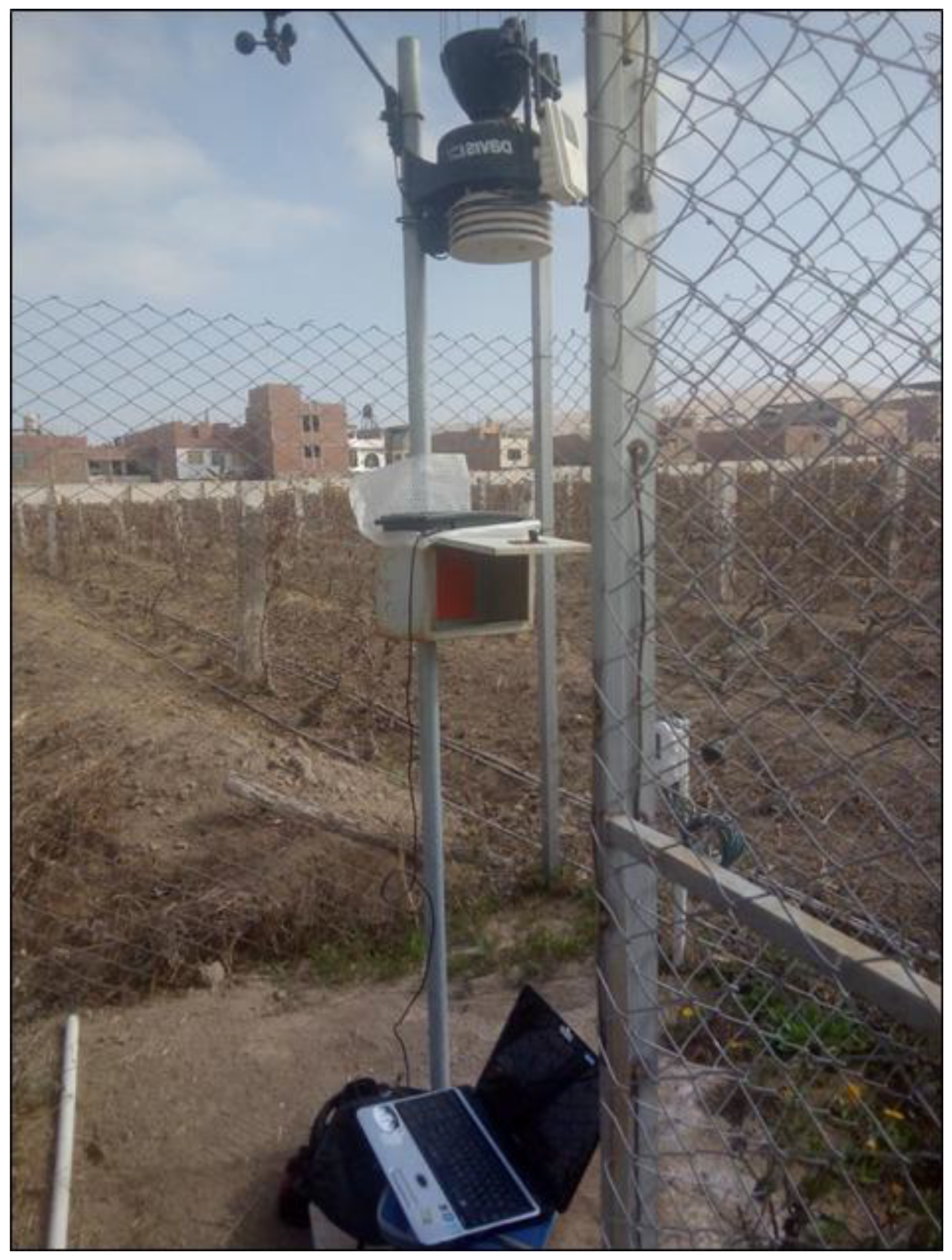
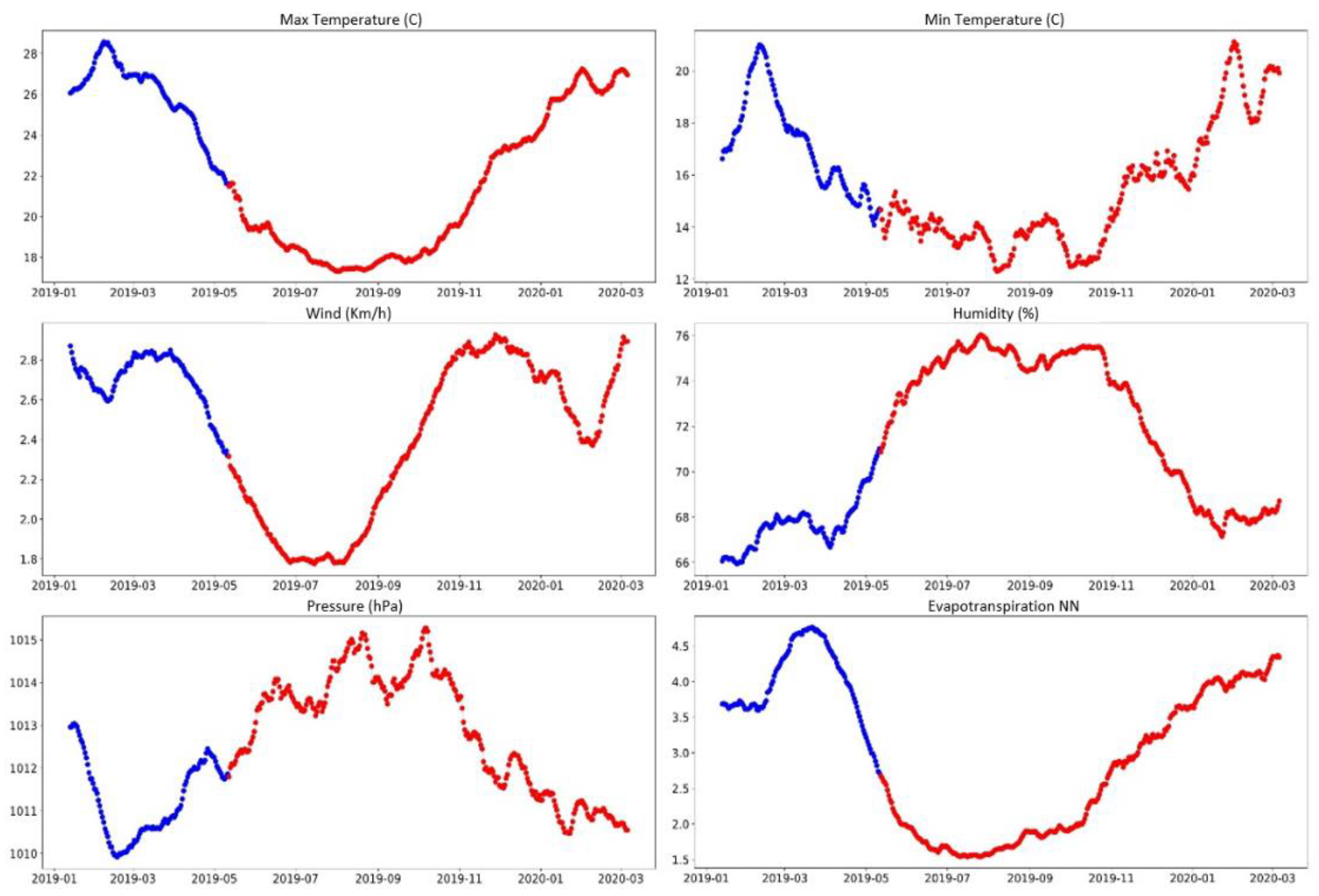
4.1. Data Description

Data were taken from an automatic weather station (Davis Instruments, Vantage Pro2 Plus), located in the La Yarada irrigation area, which we can see in Figure 1. The data correspond to the period from June 2005 to March 2020, that is, around 16 years of recording, with steps of 30 min. These data were taken from daily figures, generating 5294 records, starting from the file obtained from the automatic station and using code in Python programming language, as a pre-treatment task. The climate variables extracted from the station record were: maximum, minimum, and average temperature; relative humidity; wind speed; atmospheric pressure; precipitation; solar radiation; and evapotranspiration.

4.2. KDD (Knowledge Discovery from Data)

This work should be aligned with the computational point of view of the KDD process [31]. In the cleaning phase, we took the original dataset from the automatic weather station in xls format (Microsoft Excel 17.0), with 253,091 records (period from June 2005 to March 2020) of temperature (°C), humidity (%), wind speed (km/h), atmospheric pressure (hPa), precipitation (mm), radiation (W/m²) and evapotranspiration (mm), which were measured and recorded every 30 min. In the selection phase, we transformed the time and date variables and addressed the Null values. In the transformation phase, we performed average aggregation tasks in the case of temperature, humidity, wind speed, atmospheric pressure, radiation, and summation aggregation in the case of precipitation and evapotranspiration; grouping this especially with the date information, to have the data organized at a daily level.

As part of the transformation phase, noise cleaning of the data was carried out using the normalization technique with the mean and standard deviation. In the case of the specific climate variable of wind speed, we had an original defect, apparently caused by some (sensor) instrument calibration problem, since a lag was noted in its representation between the years 2019 and 2020. This was solved by applying data correction techniques based on related settings and interpolations. Furthermore, a moving average technique was used to smooth the data and identify any data out of range. For data exploration, we used machine learning techniques since they are efficient tools for the treatment of large volumes of data [32,33], and especially in hydrology [34,35]. We also had to convert the temporal format (time series) to a working scheme of a supervised problem. For the prediction, we used a framework based on a neural network algorithm (Multi-Layered Perceptron) widely used in hydrological forecasting [34].

4.3. The Data Science and Its Application in Hydrology

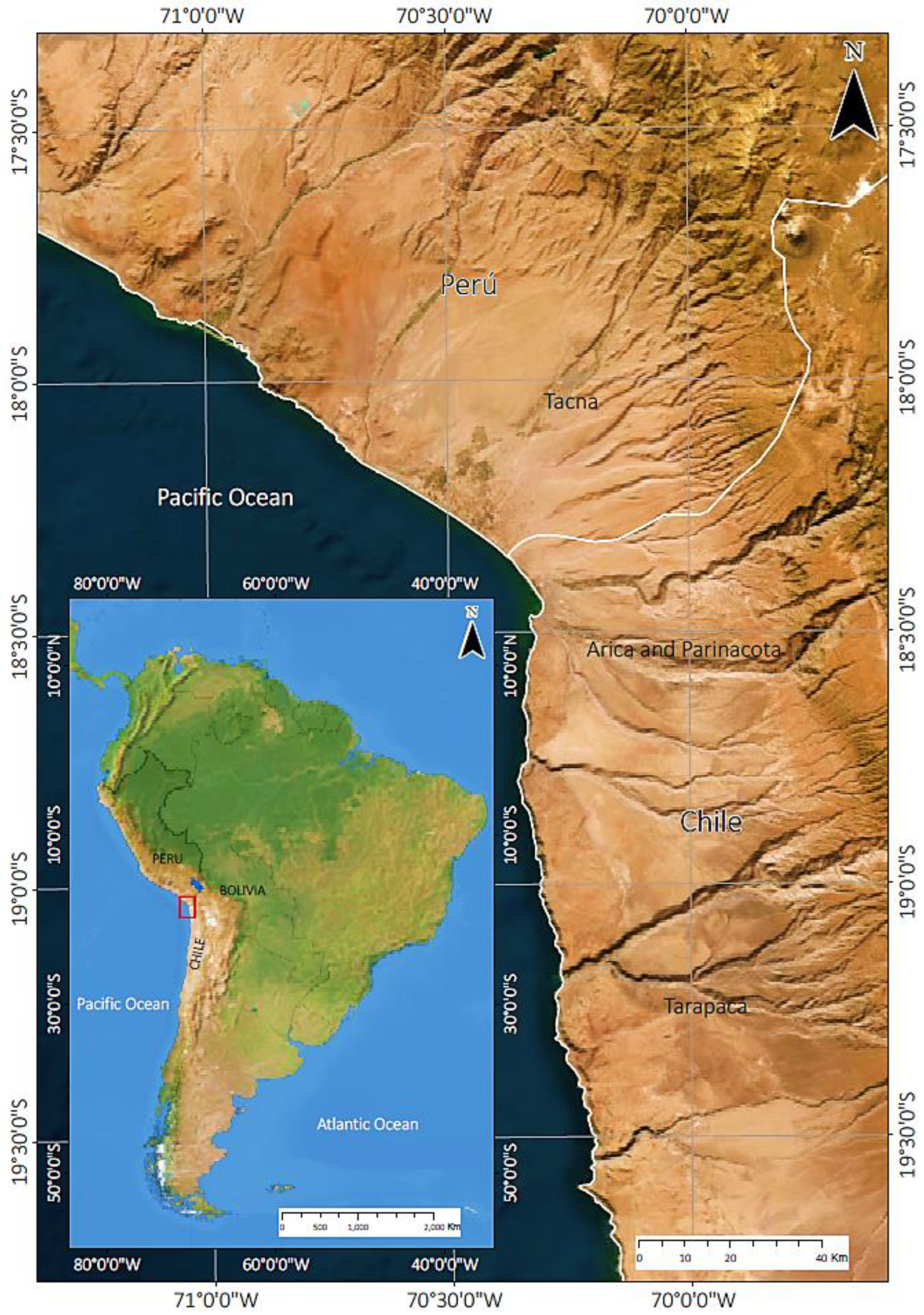
There are many previous works where different machine learning techniques have been used for the treatment, prediction, and analysis of different hydrological variables. In this way, they may inform design strategies for adequate irrigation and, thus, optimize the use of water resources.

4.4. Study Area

The study region is located in the Tacna region (Figure 2), located at the head of the Atacama Desert. It has a hyper-arid climate and is located in the extreme south of Peru and northern Chile [36,37]. In this area, the cultivation of olive trees has been developed mainly due to its low water consumption. The predominant irrigation system is by drip and the water source comes from groundwater, whose aquifer system presents water quality problems due to marine intrusion and a significant reduction in groundwater levels, since the extraction volumes exceed the recharge volume; adding to this are governance and governability problems [38,39,40].

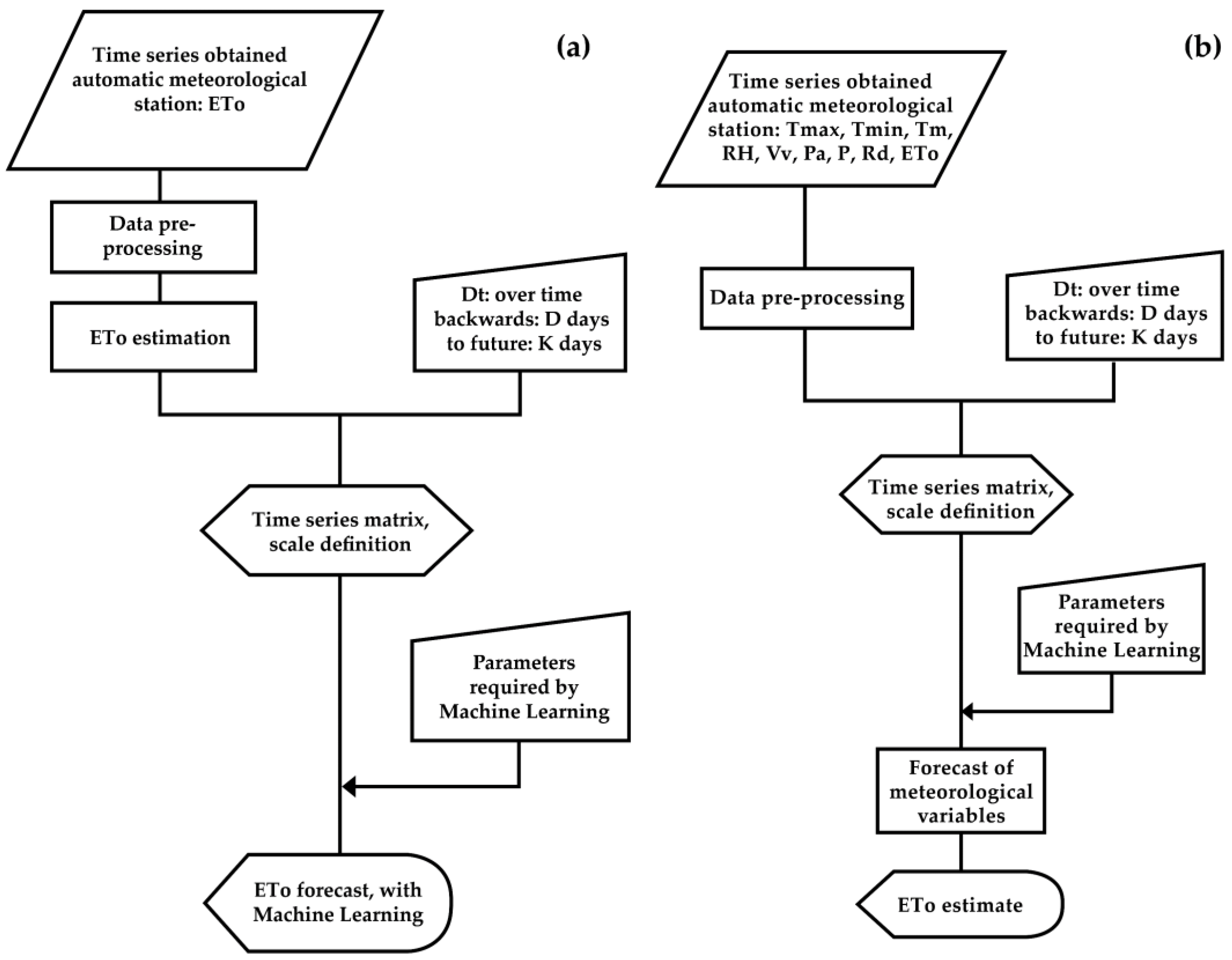
4.5. Used Approaches

Two approaches were considered to forecast the ETo. The first approach (direct approach, Figure 3a) involved obtaining the ETo that the automatic station software calculated using the Penman-Monteith equation and then applying the MLP-based deep learning model described above to directly simulate the ETo time series; obtaining the predicted values of ETo, which were subsequently contrasted and evaluated in their accuracy. The second approach (indirect approach, Figure 3b) involved applying the MLP-based deep learning model to predict each of the variables on which the ETo calculation depends, and then applying the Penman-Monteith, Hargreaves-Samani, Ritchie, and Turc equations for calculating the ETo; being of interest to evaluate its application in arid zones. A notebook was implemented in Python, using “keras” and “tensorflow” high-level libraries, as the execution engine of our deep learning model, both for its training, prediction, visualization, and evaluation.

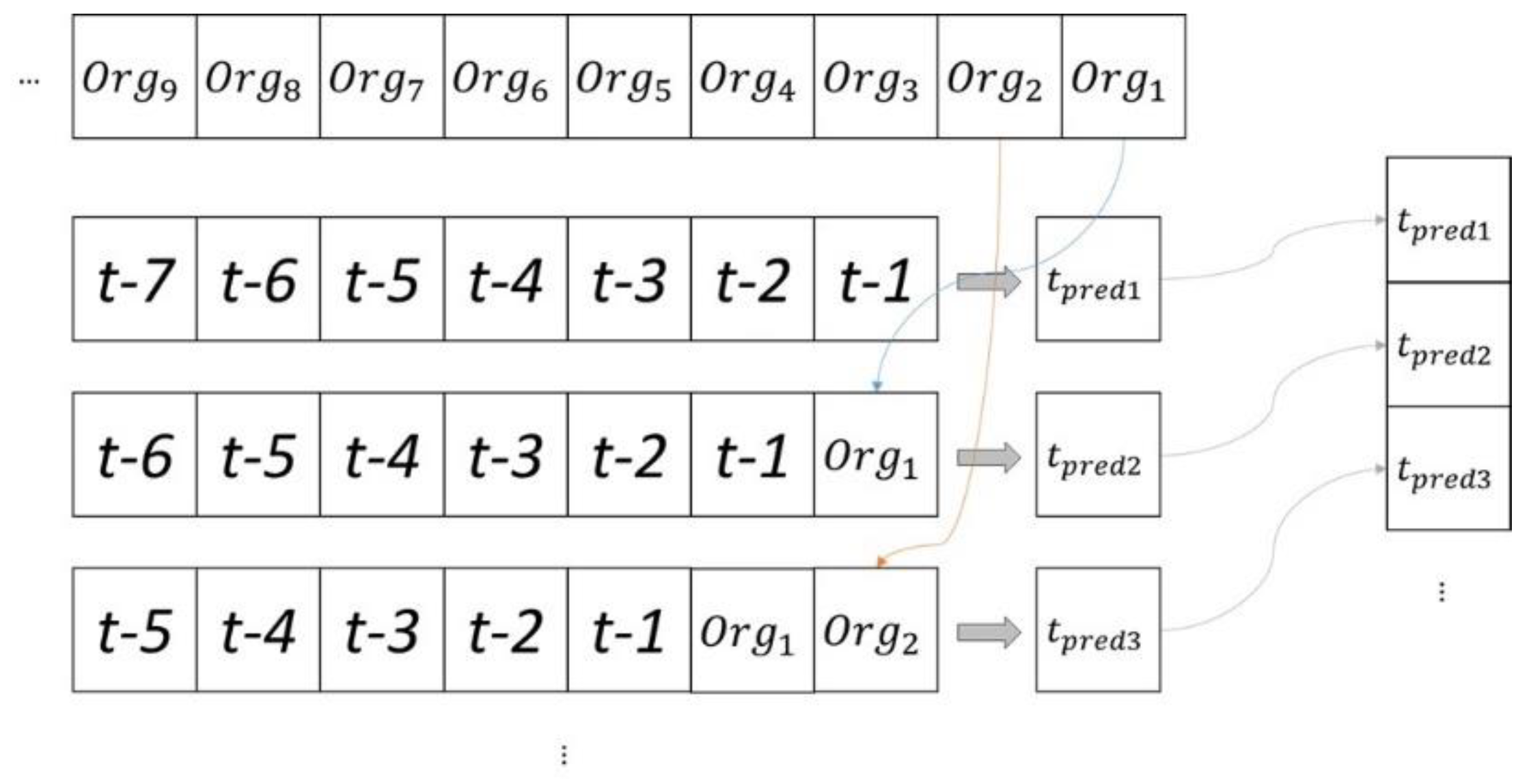
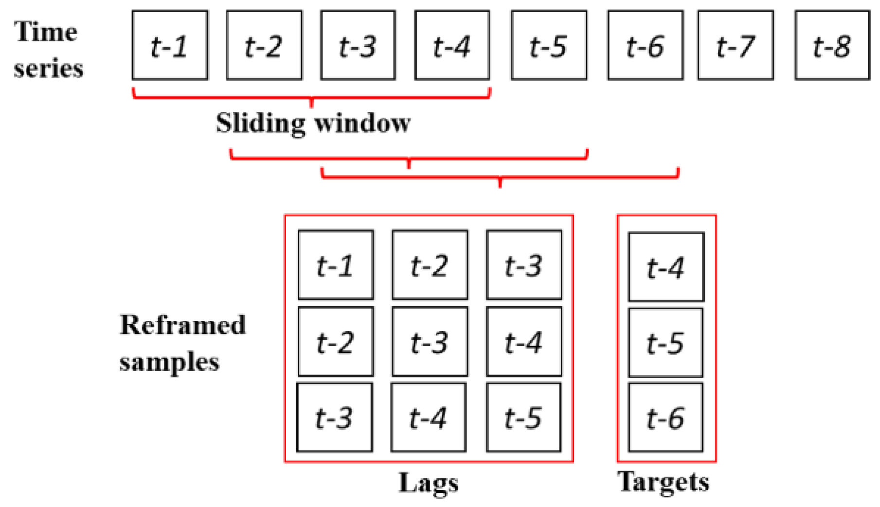
4.6. Method Applied to Avoid Prediction

After all the tests were performed and achieving intermediate results, we noticed that we could only predict one day at a time, since we were not making a “prediction over prediction”, that is, predicting values based on data that were not real but the product of our prediction using MLP. Therefore, we created a technique called the “deception method”, which involved us using the past 7 days to predict the next one, and in the next iteration we replaced the last value t-1 (which was already predicted) with the real value corresponding to the day in question; and thus, day to day, we predicted 300 days, with actual data as the input from our MLP. We called this technique the “phased and replacement model”, according to Figure 4.

4.7. Performance Measures of Predict Models

Mean Square Error (MSE): Sensitive to extreme values of the residual.

$$MSE=\frac{1}{n}{\displaystyle \sum }_{i=1}^n{\left(y_i-{\widehat{y}}_i\right)}^2$$

Root Mean Square Error (RMSE): Expressed in the same units as Loss Given Default.

$$RMSE=\sqrt{MSE}$$

Mean Absolute Error (MAE): Also known as Mean Absolute Deviation (MAD).

$$MAE=\frac{1}{n}{\displaystyle \sum }_{i=1}^n\left|y_i-{\widehat{y}}_i\right|$$

Relative Absolute Error (RAE): Ratio of MAE of the model and MAE of a simple predictor.

$$RAE=\frac{{{\displaystyle \sum }}_{i=1}^n\left|y_i-{\widehat{y}}_i\right|}{{{\displaystyle \sum }}_{i=1}^n\left|y_i-{\overline{y}}_i\right|}$$

Coefficient of determination (R-squared): In an OLS regression model with a constant term, R-squared can be interpreted as the proportion of variation in LGD that is explained by variation in the regressors.

$$R^2=1-\frac{{{\displaystyle \sum }}_{i=1}^n{\left(y_i-{\widehat{y}}_i\right)}^2}{{{\displaystyle \sum }}_{i=1}^n{\left(y_i-{\overline{y}}_i\right)}^2}$$

Adjusted coefficient of determination (adjusted R-squared): Corrected for the number of regressors (k).

$${\overline{R}}^2=1-\left(1-R^2\right)\frac{n-1}{n-k-1}$$

5. Results and Discussion

5.1. Results

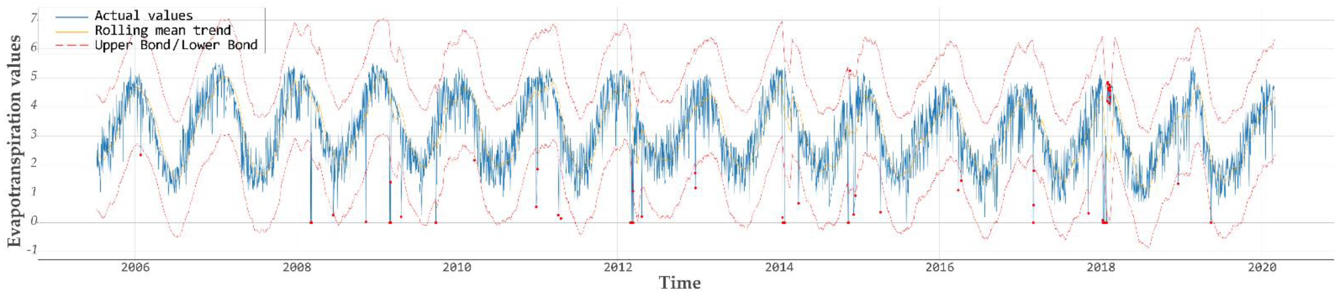
5.1.1. Data Pre-Processing Results

In the data preprocessing phase, the moving average technique was used [35] to soften and display out-of-range values, obtaining very good results as shown in Figure 5. The data and the Python code are hosted in Mendeley Data as “Data Set for climate values of Yarada-Tacna (Peru) 7 June 2005 to 6 March 2020 Period” (it includes the Dataset and Source Code in Python) [41].

Once the data were prepared for treatment as a supervised problem, both strategies suggested in Figure 4 were applied. First, for the direct approach, day-by-day evapotranspiration was predicted according to the historic values of the evapotranspiration obtained from the weather station. To avoid prediction according to the data predicted, this prediction (of one day) was made based on seven historic previous days. As we moved forward, the corresponding value was replaced by the actual data from Day 1 of the new data, obtained from the weather station, and so on, with our proposed phased and replacement model (Figure 5). The data frame that served to predict the next value was updated, according to the model of the previously trained neural network.

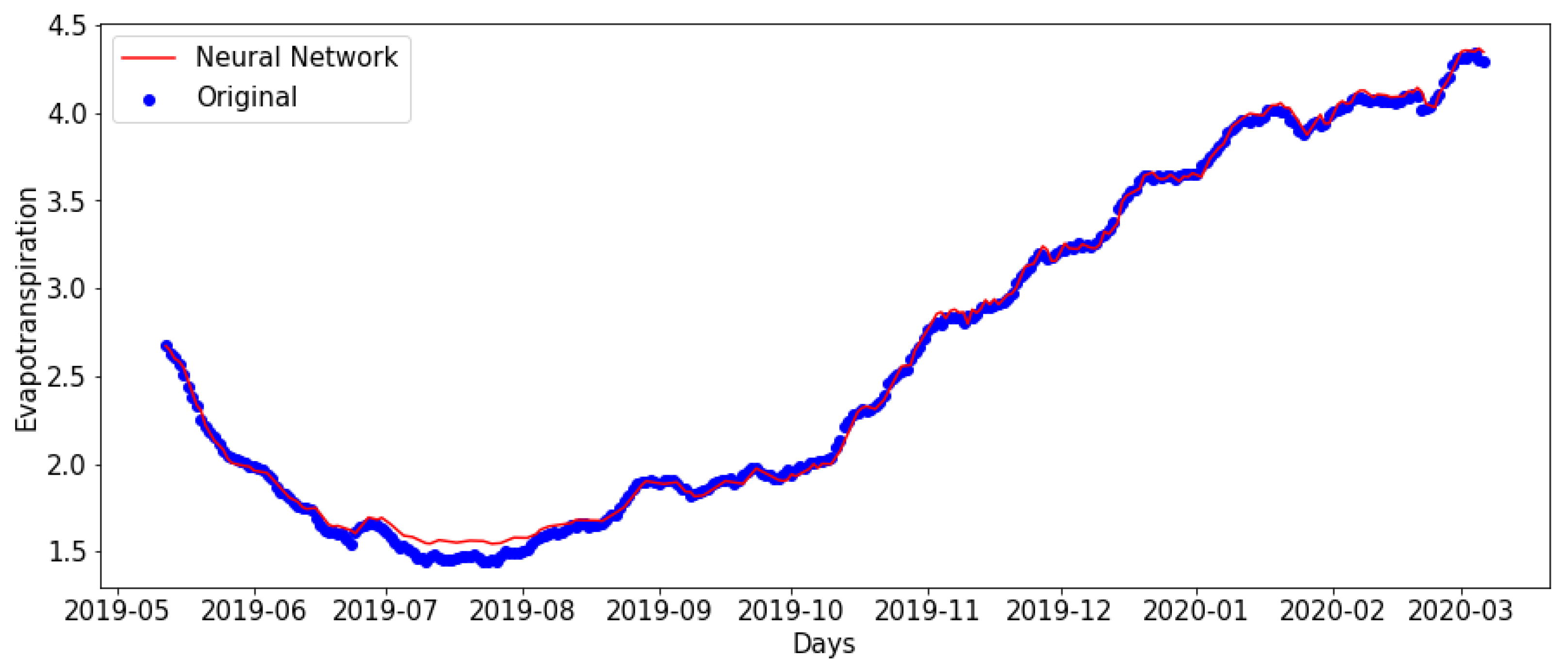
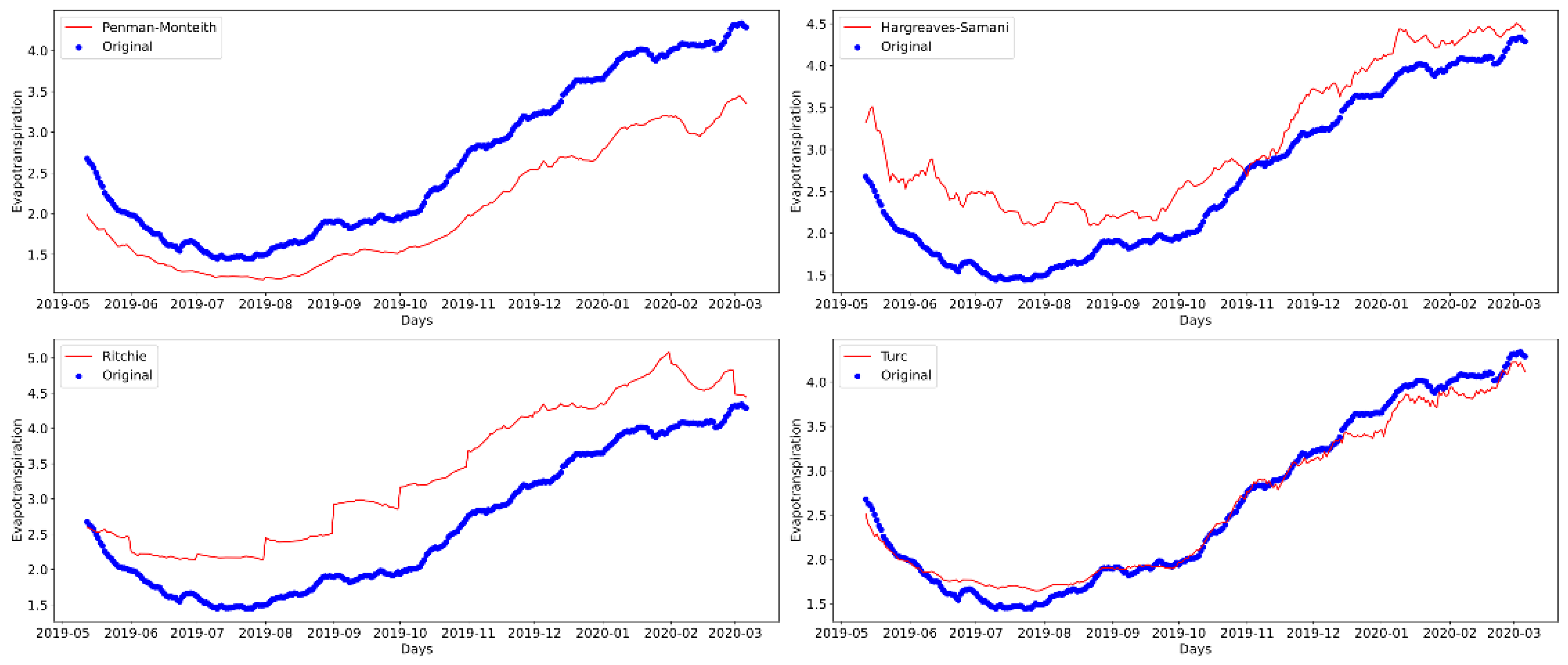
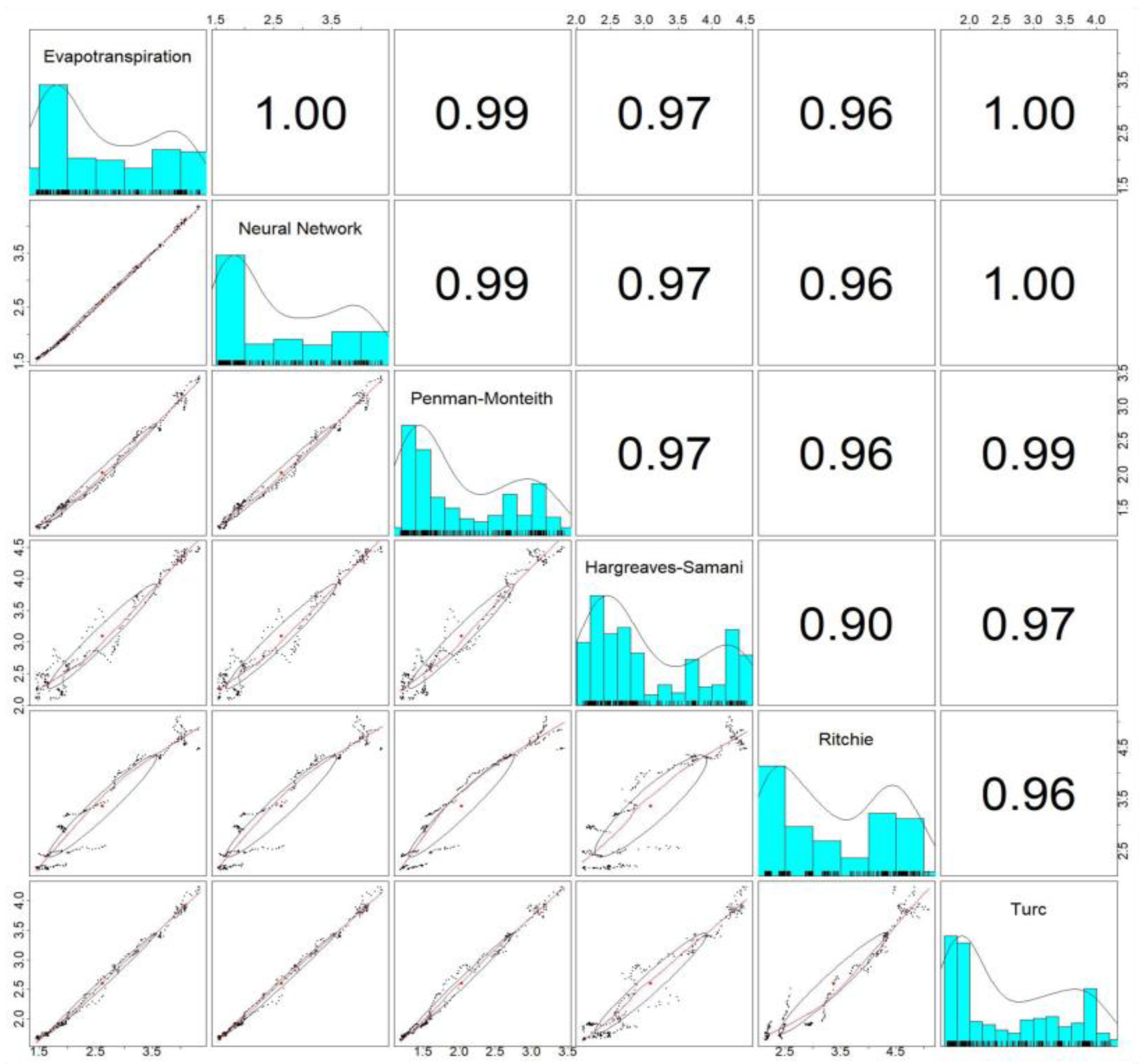
5.1.2. Applied Methods Results

For the indirect approach, we used the daily prediction of other climate variables (temperature, pressure, radiation, wind, humidity) to apply the Penman-Monteith equation as well as the Hargreaves-Samani, Ritchie, and Turc equations. We considered it important to verify the precision of each one of them for the specific data of our study region. This allowed us to predict 300 days, one at a time, and under regular conditions; and allowed us to predict daily data with great precision. Figure 6 shows the prediction using the neural network contrasted with the actual data; observing a good approximation for the direct approach.

Precision indicators of the model based on the neural network for the direct approach are: MAE = 0.03312 (Media Absolute Error); MSE = 0.001875 (Media Square Error); RMSE = 0.043303 (Root of the MSE); and RAE = 0.015553 (Relative Absolute error).

By having close values between the MAE and RMSE, we can infer that there is an error evenly distributed and no significant outliers, which is confirmed as we can visualize the comparative curve of the predicted values with the actual values. In addition, for the methods based on gradients optimization, it is convenient to consider the RMSE to set some parameters in the learning rate, which we did reiteratively.

The MAE is a low value (MAE = 0.033) and represents an element of penalty for large errors; that is, it is less sensitive to atypical errors, which means that there are no large errors.

Then we apply scheme (b), in which we are in charge of predicting the values of the climate variables using our model based on neural networks, and then, based on those predictions, calculate the different equations in the literature (Penman-Monteith, Hargreaves-Samani, Ritchie, and Turc) and compare their errors and correlation coefficients with the actual data.

In the following graphs, we show the prediction of the different climate variables that will serve as the input to apply the different previously mentioned equations for calculating the ETo, and compare their precision. Figure 7 shows the prediction for the temperature variable, minimum and maximum, humidity, wind speed, pressure, and radiation in 300 days, specifically using the MLP neural networks.

With the predicted climate variables, and using our proposal for a phased and exchange model, we calculated a total of 300 values daily (Figure 7). The evapotranspiration was calculated using different equations, established as Penman-Monteith, Hargreaves-Samani, Ritchie, and Turc, and we compared these results to the actual prediction and analyzed its accuracy and performance, as can be seen in Figure 8.

In

Table 2. Metrics results.

Indicator	Neural Network	Penman-Monteith	Hargreaves-Samani	Ritchie	Turc
MAE	0.033	0.586	0.467	0.749	0.104
MSE	0.002	0.411	0.285	0.632	0.016
RMSE	0.043	0.641	0.534	0.795	0.128
RAE	0.016	0.230	0.192	0.285	0.046
R-Squared	0.998	0.550	0.689	0.309	0.982

MAE = Mean absolute error; MSE = Mean square error; RMSE = root of the MSE; and RAE = Relative absolute error.

, we can see the summary of the various indicators of errors and accuracy factors under the indirect approach. In this second approach, climate variables that serve as the basis for calculating the ETo were predicted. The precision indicators show good conditions in their process, with MAE, MSE, RMSE, and RAE values, which guarantee the suitability of the predicted variables.

According to the MAE, being the most robust reference for our purpose as it is less sensitive to atypical values, we established that the best prediction for evapotranspiration is that of Turc, having a MAE of 0.104, as opposed to Hargreaves-Samani with a MAE of 0.467, Ritchie with a MAE of 0.749, and finally, Penman-Monteith with a MAE of 0.586. It should be noted that we do not consider the prediction based on neural networks (MLP) since in the application of scheme (b), we only use the equations to calculate the value of evapotranspiration.

Figure 9 shows a comparative summary of the correlation factors between the methods used.

5.2. Discussion

We found that deep learning using neural network algorithms, such as Multi-Layer Perceptron, may be used for the prediction of time series as in this case, but it is necessary to emphasize that one of the main problems in the classification of time series is given by its structure, generally, when classifying phenomena described by attributes. Their order does not affect the result; however, the time series preserve order or temporality, which does not allow for a change in the position of the data. Thus, algorithms that work with attributes cannot be applied in this type of problem [42]. This was previously solved by adapting the time series to the format of a supervised problem (Figure 10).

Thus the “data frame” or data structure with two dimensions that stores the data of the variables is defined as shown in

Table 3. Transformation of time series to supervised problem format.

t-7	t-6	t-5	t-4	t-3	t-2	t-1	t
−0.32	−0.32	−0.33	0.35	−0.35	−0.36	−0.36	0.35
−0.32	−0.33	−0.35	0.35	−0.36	−0.36	−0.35	0.36
−0.33	−0.35	−0.35	0.36	−0.36	−0.35	−0.36	0.36
−0.35	−0.35	−0.36	0.36	−0.35	−0.36	−0.36	0.36
−0.35	−0.36	−0.36	0.35	−0.36	−0.36	−0.36	0.37

, where “t” represents the predicted value. The values are normalized for the hyperbolic tangent, which is the function of the neural network activation whose input values are between −1 and 1.

The results indicate that the prediction of evapotranspiration values using neural networks has a lower error than the traditional formulations of Penman-Monteith [25], Hargreaves [22], Ritchie [23] and Turc [24].

6. Conclusions

This work demonstrates the feasibility of forecasting the short-term daily ETo, which is required for irrigation water management purposes, based on the Penman-Monteith, Hargreaves-Samani, Ritchie, and Turc equations. Two approaches were tested using the Feedforward neural network algorithm (Multi-Layered Perceptron). The first approach, the direct approach, involves estimating future ETo time series from historical data obtained from the automatic station. The second approach, the indirect approach, considers forecasting the weather data necessary for the ETo equations, maximum temperature, minimum temperature, wind speed, humidity, pressure, and evapotranspiration on a daily level using the aforementioned machine learning and, subsequently, using these predicted values to estimate future ETo values.

The model precision indicators based on neural networks for the direct approach are values that guarantee a good precision in the forecast, MAE = 0.033, MSE = 0.002, RMSE = 0.043, and RAE = 0.016. Regarding the indirect approach, the prediction of the climate variables that were used to calculate the ETo was carried out. The precision indicators show optimal conditions in their process and guarantee the suitability of the predicted variables.

The results indicate that using the approaches proposed in this study makes it possible to forecast up to 300 days of daily ETo in advance within a reasonable range of time. Furthermore, the use of this methodology provides an additional estimate of the expected variability values for each forecast day, which ensures a very good estimate of ETo. The forecast with more than 300 days in advance is affected by the relationship of the value of the time series with the previous ones. Therefore, the accuracy of the predicted ETo decreases over time.

Comparing the performance of the approaches and the machine learning used, the results obtained indicate that, despite the similar performance of the two proposed approaches, the indirect approach provides better ETo forecasting capabilities for longer time intervals than the direct approach. This result is because it only uses weather parameters required for ETo equations to model and predict behavior, while for the direct approach, the machine learning model is required to forecast the combined effect of the climate variables’ trend on the resulting ETo. Therefore, the indirect approximation may be extended to other equations of ETo.

References

1. Wang, H.; Yan, H.; Zeng, W.; Lei, G.; Ao, C.; Zha, Y. A Novel Nonlinear Arps Decline Model with Salp Swarm Algorithm for Predicting Pan Evaporation in the Arid and Semi-Arid Regions of China. J. Hydrol. 2020, 582, 124545. [Google Scholar] [CrossRef]
2. Fan, J.; Yue, W.; Wu, L.; Zhang, F.; Cai, H.; Wang, X.; Lu, X.; Xiang, Y. Evaluation of SVM, ELM and Four Tree-Based Ensemble Models for Predicting Daily Reference Evapotranspiration Using Limited Meteorological Data in Different Climates of China. Agric. For. Meteorol. 2018, 263, 225–241. [Google Scholar] [CrossRef]
3. Goyal, M.K.; Bharti, B.; Pham, Q.N.; Adamowski, J.; Pandey, A. Modeling of Daily Pan Evaporation in Sub Tropical Climates Using ANN, LS-SVR, Fuzzy Logic, and ANFIS. Expert Syst. Appl. 2014, 41, 5267–5276. [Google Scholar] [CrossRef]
4. Guan, Y.; Mohammadi, B.; Pham, Q.; Adarsh, S.; Balkhair, K.S.; Khalil, U.R.; Rahman, U.; Nguyen, T.T.L.; Linh, T.T.; Tri, Q. A Novel Approach for Predicting Daily Pan Evaporation in the Coastal Regions of Iran Using Support Vector Regression Coupled with Krill Herd Algorithm Model. Theor. Appl. Climatol. 2020, 142, 349–367. [Google Scholar] [CrossRef]
5. Manikumari, N.; Vinodhini, G.; Murugappan, A. Modelling of Reference Evapotransipration Using Climatic Parameters for Irrigation Scheduling Using Machine Learning. ISH J. Hydraul. Eng. 2020, 28, 272–281. [Google Scholar]
6. Raza, A.; Shoaib, M.; Khan, A.; Baig, F.; Faiz, M.A.; Khan, M.M. Application of Non-Conventional Soft Computing Approaches for Estimation of Reference Evapotranspiration in Various Climatic Regions. Theor. Appl. Climatol. 2020, 139, 1459–1477. [Google Scholar] [CrossRef]
7. Torres, A.F.; Walker, W.R.; McKee, M. Forecasting Daily Potential Evapotranspiration Using Machine Learning and Limited Climatic Data. Agric. Water Manag. 2011, 98, 553–562. [Google Scholar] [CrossRef]
8. Silva, D.; Meza, F.J.; Varas, E. Estimating Reference Evapotranspiration (ETo) Using Numerical Weather Forecast Data in Central Chile. J. Hydrol. 2010, 382, 64–71. [Google Scholar] [CrossRef]
9. Adamala, S. Temperature Based Generalized Wavelet-Neural Network Models to Estimate Evapotranspiration in India. Inf. Process. Agric. 2018, 5, 149–155. [Google Scholar] [CrossRef]
10. Adeloye, A.J.; Rustum, R.; Kariyama, I.D. Neural Computing Modeling of the Reference Crop Evapotranspiration. Environ. Model. Softw. 2012, 29, 61–73. [Google Scholar] [CrossRef]
11. Antonopoulos, V.Z.; Antonopoulos, A.V. Daily Reference Evapotranspiration Estimates by Artificial Neural Networks Technique and Empirical Equations Using Limited Input Climate Variables. Comput. Electron. Agric. 2017, 132, 86–96. [Google Scholar] [CrossRef]
12. Laqui, W.; Zubieta, R.; Rau, P.; Mejía, A.; Lavado, W.; Ingol, E. Can Artificial Neural Networks Estimate Potential Evapotranspiration in Peruvian Highlands? Model. Earth Syst. Environ. 2019, 5, 1911–1924. [Google Scholar] [CrossRef]
13. David Rumelhart Geoffrey Hinton, R.W. Learning Representations by Back-Propagating Errors. Nature 1986, 323, 533–536. [Google Scholar]
14. Zhang, S.; Zhang, S.; Wang, B.; Habetler, T.G. Deep Learning Algorithms for Bearing Fault Diagnosticsx—A Comprehensive Review. IEEE Access 2020, 8, 29857–29881. [Google Scholar] [CrossRef]
15. Car, Z.; Šegota, S.B.; Anđelić, N.; Lorencin, I.; Mrzljak, V. Modeling the Spread of COVID-19 Infection Using a Multilayer Perceptron. Comput. Math. Methods Med. 2020, 2020, 5714714. [Google Scholar] [CrossRef] [PubMed]
16. Shen, Z.; Zhang, Y.; Lu, J.; Xu, J.; Xiao, G. A Novel Time Series Forecasting Model with Deep Learning. Neurocomputing 2020, 396, 302–313. [Google Scholar] [CrossRef]
17. Kumar, M.; Raghuwanshi, N.S.; Signh, R.; Wallender, W.W.; Pruitt, W.O. Estimating of Evapotranspiration Using Artificial Neural Network. J. Irrig. Drain. Eng. 2002, 128, 224–233. [Google Scholar] [CrossRef]
18. Machaca-Apaza, L.C. Estimación de la Evapotranspiración de Referencia Utilizando Modelos de Redes Neuronales Artificiales En Función de Elementos Climáticos en la Cuenca Del Rio Huancané. Bachelor’s Thesis, Universidad Nacional del Altiplano, Puno, Peru, 2016. [Google Scholar]
19. Yang, Y.; Chen, R.; Han, C.; Liu, Z. Evaluation of 18 Models for Calculating Potential Evapotranspiration in Different Climatic Zones of China. Agric. Water Manag. 2021, 244, 106545. [Google Scholar] [CrossRef]
20. Nearing, G.S.; Kratzert, F.; Sampson, A.K.; Pelissier, C.S.; Klotz, D.; Frame, J.M.; Prieto, C.; Gupta, H.V. What Role Does Hydrological Science Play in the Age of Machine Learning? Water Resour. Res. 2020, 57, e2020WR028091. [Google Scholar] [CrossRef]
21. Kaya, Y.Z.; Zelenakova, M.; Üneş, F.; Demirci, M.; Hlavata, H.; Mesaros, P. Estimation of Daily Evapotranspiration in Košice City (Slovakia) Using Several Soft Computing Techniques. Theor. Appl. Climatol. 2021, 144, 287–298. [Google Scholar] [CrossRef]
22. Hargreaves, G.H.; Samani, Z.A. Reference Crop Evapotranspiration from Temperature. Appl. Eng. Agric. 1985, 1, 96–99. [Google Scholar] [CrossRef]
23. Ritchie, J.T. Model for Predicting Evaporation from a Row Crop with Incomplete Cover. Water Resour. Res. 1972, 8, 1204–1213. [Google Scholar] [CrossRef]
24. Lecarpentier, C. L’évapotranspiration Potentielle et Ses Implications Géographiques (Suite). Ann. Georgr. 1975, 84, 385–414. [Google Scholar] [CrossRef]
25. Valiantzas, J.D. Simplified Forms for the Standardized FAO-56 Penman-Monteith Reference Evapotranspiration Using Limited Weather Data. J. Hydrol. 2013, 505, 13–23. [Google Scholar] [CrossRef]
26. Babakos, K.; Papamichail, D.; Tziachris, P.; Pisinaras, V.; Demertzi, K.; Aschonitis, V. Assessing the Robustness of Pan Evaporation Models for Estimating Reference Crop Evapotranspiration during Recalibration at Local Conditions. Hydrology 2020, 7, 62. [Google Scholar] [CrossRef]
27. Giles-Hansen, K.; Wei, X.; Hou, Y. Dramatic Increase in Water Use Efficiency with Cumulative Forest Disturbance at the Large Forested Watershed Scale. Carbon Balance Manag. 2021, 16, 6. [Google Scholar] [CrossRef] [PubMed]
28. Efron, B.; Hastie, T. Computer Age Statistical Inference; Cambridge Univesity Press: Cambridge, UK, 2016. [Google Scholar]
29. Ruder, S. An Overview of Gradient Descent Optimization Algorithms. arXiv 2016, arXiv:1609.04747. [Google Scholar]
30. Abdolrasol, M.G.M.; Hussain, S.M.S.; Ustun, T.S.; Sarker, M.R.; Hannan, M.A.; Mohamed, R.; Ali, J.A.; Mekhilef, S.; Milad, A. Artificial Neural Networks Based Optimization Techniques: A Review. Electronics 2021, 10, 2689. [Google Scholar] [CrossRef]
31. Fayyad, U.; Piatetsky-Shapiro, G.; Smyth, P. The KDD Process for Extracting Useful Knowledge from Volumes of Data. Commun. ACM 1996, 39, 27–34. [Google Scholar] [CrossRef]
32. Hong, W.C. Rainfall Forecasting by Technological Machine Learning Models. Appl. Math. Comput. 2008, 200, 41–57. [Google Scholar] [CrossRef]
33. Ahmad, S.; Kalra, A.; Stephen, H. Estimating Soil Moisture Using Remote Sensing Data: A Machine Learning Approach. Adv. Water Resour. 2010, 33, 69–80. [Google Scholar] [CrossRef]
34. Feng, L.; Hong, W. On Hydrologic Calculation Using Artificial Neural Networks. Appl. Math. Lett. 2008, 21, 453–458. [Google Scholar] [CrossRef] [Green Version]
35. Bühlmann, P. ELSEVEX Moving-Average Representation of Autoregressive Approximations. Stoch. Process. Appl. 1995, 60, 331–342. [Google Scholar] [CrossRef]
36. Pino, E.; Tacora, P.; Steenken, A.; Alfaro, L.; Valle, A.; Chávarri, E.; Ascencios, D.; Marcacuzco, J.A.M. Efecto de las Características Ambientales y Geológicas Sobre la Calidad del Agua en la Cuenca del Río Caplina, Tacna, Perú. Tecnol. Cienc. Agua 2017, 8, 77–99. [Google Scholar] [CrossRef]
37. Pino-Vargas, E.; Chávarri-Velarde, E.; Ingol-Blanco, E.; Mejía, F.; Cruz, A.; Vera, A. Impacts of Climate Change and Variability on Precipitation and Maximum Flows in Devil’s Creek, Tacna, Peru. Hydrology 2022, 9, 10. [Google Scholar] [CrossRef]
38. Vera, A.; Pino-Vargas, E.; Verma, M.P.; Chucuya, S.; Chávarri, E.; Canales, M.; Torres-Martínez, J.A.; Mora, A.; Mahlknecht, J. Hydrodynamics, Hydrochemistry, and Stable Isotope Geochemistry to Assess Temporal Behavior of Seawater Intrusion in the la Yarada Aquifer in the Vicinity of Atacama Desert, Tacna, Peru. Water 2021, 13, 3161. [Google Scholar] [CrossRef]
39. Chucuya, S.; Vera, A.; Pino-Vargas, E.; Steenken, A.; Mahlknecht, J.; Montalván, I. Hydrogeochemical Characterization and Identification of Factors Influencing Groundwater Quality in Coastal Aquifers, Case: La Yarada, Tacna, Peru. Int. J. Environ. Res. Public Health 2022, 19, 2815. [Google Scholar] [CrossRef] [PubMed]
40. Narvaez-Montoya, C.; Torres-Martínez, J.A.; Pino-Vargas, E.; Cabrera-Olivera, F.; Loge, F.J.; Mahlknecht, J. Predicting Adverse Scenarios for a Transboundary Coastal Aquifer System in the Atacama Desert (Peru/Chile). Sci. Total Environ. 2022, 806, 150386. [Google Scholar] [CrossRef]
41. Pino-Vargas, E.; Taya-Acosta, E.; Torres-Rúa, A. Data Set for Climate Values of Yarada-Tacna(Perú) 7-6-2005 to 6-3-2020 Period, Tacna. 2021. Available online: https://data.mendeley.com/datasets/df46xjw62v/1 (accessed on 30 April 2021).
42. Santos-Camacho, E.A.; Figueroa-Nazuno, J.G.; Eguía, J.C.C. Clasificador No Supervisado Para Series de Tiempo Unsupervised Classifier for Time Series. Res. Comput. Sci. 2015, 105, 21–29. [Google Scholar] [CrossRef]
Figure 1. Weather station Davis Instruments, Vantage Pro2 Plus.
Agriculture 12 01971 g001
Figure 2. Location of the study area.
Agriculture 12 01971 g002
Figure 3. ETo forecasting approaches: (a) Direct approach; (b) Indirect approach; adapted from Torres et al. (2011) [7].
Agriculture 12 01971 g003
Figure 4. Proposal of the phased and replacement model to avoid prediction over prediction.
Agriculture 12 01971 g004
Figure 5. Visualization of out-of-range evapotranspiration values using moving averages.
Agriculture 12 01971 g005
Figure 6. Comparison of the 300-day ETo prediction using a neural network with the actual data (Direct approach).
Agriculture 12 01971 g006
Figure 7. Blue color, original data; red color, predicted data. The figure shows the prediction for 300 days, using neural networks, of Maximum Temperature (°C), Minimum Temperature (°C), Wind Speed (km/hr), Moisture (%), Pressure (hPa), and Evapotranspiration (mm).
Agriculture 12 01971 g007
Figure 8. ETo calculated using the Penman-Monteith, Hargreaves-Samani, Ritchie, and Turc equations for 300 days, using climate variables predicted with neural networks compared with the actual data.
Agriculture 12 01971 g008
Figure 9. Comparison of the ETo as compared to the application of the Penman-Monteith, Hargreaves-Samani, Ritchie, and Turc equations.
Agriculture 12 01971 g009
Figure 10. Transposing data from time format to supervised problem.
Agriculture 12 01971 g010