Article

Seasonal and Diurnal Cycles of Surface Boundary Layer and Energy Balance in the Central Andes of Perú, Mantaro Valley

by
José Luis Flores-Rojas
1,*,†,
Joan Cuxart
2,
Manuel Piñas-Laura
1,
Stephany Callañaupa
1,
Luis Suárez-Salas
1,
Shailendra Kumar
1,
Aldo S. Moya-Alvarez
1 and
Yamina SIlva
1
1
Geophysical Institute of Perú, Lima 15012, Peru
2
Grup de Meteorologia, Departament de Física, Universitat de les Illes Balears, 07122 Palma de Mallorca, Spain
*
Author to whom correspondence should be addressed.
Current address: Calle Badajoz 169 Urb, Mayorazgo IV Etapa, Ate, Lima 15012, Peru.
Atmosphere 2019, 10(12), 779; https://doi.org/10.3390/atmos10120779
Submission received: 13 October 2019 / Revised: 15 November 2019 / Accepted: 21 November 2019 / Published: 5 December 2019
(This article belongs to the Section Biosphere/Hydrosphere/Land–Atmosphere Interactions)

Abstract

:
The present study presents a detailed analysis of the diurnal and monthly cycles the surface boundary layer and of surface energy balance in a sparse natural vegetation canopy on Huancayo observatory (12.04 S, 75.32 W, 3313 m ASL), which is located in the central Andes of Perú (Mantaro Valley) during an entire year (May 2018–April 2019). We used a set of meteorological sensors (temperature, relative humidity, wind) installed in a gradient tower 30 m high, a set of radiative sensors to measure all irradiance components, and a set of tensiometers and heat flux plate to measure soil moisture, soil temperatures and soil heat flux. To estimate turbulent energy fluxes (sensible and latent), two flux–gradient methods: the aerodynamic method and the Bowen-ratio energy-balance method were used. The ground heat flux at surface was estimated using a molecular heat transfer equation. The results show minimum mean monthly temperatures and more stable conditions were observed in June and July before sunrise, while maximum mean monthly temperatures in October and November and more unstable conditions in February and March. From May to August inverted water vapor profiles near the surface were observed (more intense in July) at night hours, which indicate a transfer of water vapor as dewfall on the surface. The patterns of wind direction indicate well-defined mountain–valley circulation from south-east to south-west especially in fall–winter months (April–August). The maximum mean monthly sensible heat fluxes were found in June and September while minimum in February and March. Maximum mean monthly latent heat fluxes were found in February and March while minimum in June and July. The surface albedo and the Bowen ratio indicate semi-arid conditions in wet summer months and extreme arid conditions in dry winter months. The comparisons between sensible heat flux ( Q H ) and latent heat flux ( Q E ), estimated by the two methods show a good agreement (R 2 above 0.8). The comparison between available energy and the sum of Q E and Q H fluxes shows a good level of agreement (R 2 = 0.86) with important imbalance contributions after sunrise and around noon, probably by advection processes generated by heterogeneities on the surface around the Huancayo observatory and intensified by the mountain–valley circulation.

1. Introduction

The lower natural boundary of the atmosphere is the earth’s surface. Transport processes of mass and energy between the atmosphere and the earth’s surface modify the lowest part of the atmosphere, creating the planetary boundary layer (PBL) [1], which plays an important role in many fields, including weather forecasting and climate, mesoscale meteorology, hydrology, agricultural meteorology, and air pollution [2]. In particular, agricultural meteorology and hydrology are concerned with processes such as evaporation, dewfall, frost formation, as well as with dry deposition of natural gases and pollutants to crops. All these processes are associated with the state of the PBL, the energy balance at the surface, and the intensity of turbulence [3].
A surface layer (SL) is the region at the bottom of the PBL where turbulent fluxes and stresses vary by less than 10% of their magnitude. In convective diurnal conditions, the SL can have a height of around 100 m in stable nocturnal conditions of around 10 m [1,3]. The study of this lower layer (SL) is very important to understand the strong interactions between the surface and the atmosphere and to estimate the turbulent transports of momentum, heat, and water vapor with enough accuracy to improve the study at a much larger scale in other parts of the atmosphere [4,5]. Two basic profile methods are used to estimate the surface turbulent energy fluxes: the aerodynamic and the Bowen-ratio energy balance, and both use the similarity principle, which consider the diffusion coefficients for momentum, heat, and water vapor to be equivalent [6,7,8,9].
In the Andean region of South America, energy balance, evapo-transpiration, surface albedo and dew deposition have been studied for the arid and the topographically complex Elqui valley at south of the hyper-arid Atacama Desert (Chile) [10]. For the Elqui valley, the daytime albedo of the natural vegetation was found to be about 0.17 and for the Bowen ratio 11, which correspond to the value in arid areas. Furthermore, the meteorological values were found to be strongly depend on the main features of the surface terrain over which the measurements were taken [11,12]. In fact, turbulent sensible and latent heat fluxes, net irradiance, and ground fluxes strongly depend on the characteristics of the surface, such as soil texture, vegetation cover, and roughness [13,14].
Several recent studies have shown the heterogeneity of the surface terrain at the hectometer scale can facilitate transport of energy, mass, and momentum due to turbulent mixing or advective local transports [15,16]. The lack of energy-balance closure typically found to be in the range of 10% to 35% [17] and mostly related to instrumental uncertainties, lateral contributions induced by heterogeneities of surface terrain, and some missing sources or sinks [18].
In the central Andes of Perú, on the Huancayo observatory, the thirty-three year-old (1973–2006) climatology [19], shows a well-defined seasonal cycle of precipitation with a wet season from September to April (80% from December to March) and a dry season between May and August [20,21,22,23,24]. Further, the minimum temperature (T min ) was found to follow a seasonal pattern ranging from 7 C in December–February to 0 C in June–July. In contrast, the maximum temperature (T max ) presents a low seasonal variability with maximum in February (18.5 C) and October-November (21.0 C). Also the physical controls on frost events in the Huancayo observatory was analyzed using in situ observations and energy flux models [19]. The results show low cloud cover, surface-specific humidity, and soil moisture are key factors that control the day-to-day variability of minimum temperature, which is more pronounced in the dry/cool season. However, lack of information on the components of the energy budget found to be an important source of uncertainty. Moreover, a recent contribution evaluated the sensitivity of the precipitation forecast in the central Andes of Perú of the Weather Research and Forecasting (WRF) model to change the planetary boundary layer (PBL) schemes [25]. The results show the schemes that generated the most rainfall were those of a more unstable boundary layer with weaker wind speeds, at least with easterly winds.
Motivated by these considerations, the present contribution tries to partially cover the lack of information of the seasonal and diurnal cycles of the surface boundary layer and of the energy-balance components in the Huancayo observatory located in central Andes of Perú using a set of sensors to measure temperature, relative humidity, and wind at different heights. Further, a set of irradiance sensors were employed to measure the irradiance components and a set of tensiometers and a heat flux plate to measure soil moisture, soil temperatures, and soil heat flux. To estimate the turbulent energy fluxes (sensible and latent), this study used two flux–gradient methods: the aerodynamic method and the Bowen-ratio energy-balance method. The ground heat flux at the surface was estimated using a molecular heat transfer equation.
Some important applications of these results lie in the local function that land-atmosphere interactions play in the rainfall process [26] and in the development of frost events [19] because the magnitude of the surface energy fluxes, the soil water content, and the effect of surface albedo on the dynamics of the PBL. Moreover, the seasonal and diurnal cycles of the boundary layer and of the energy budget components have been observed to have a critical influence on the climate system; however, these are not conveniently simulated by numerical regional or climate models [27,28]. Consequently, an accurate estimation of the cycles of the SBL and of surface energy fluxes is required to improve forecast predictions and to understand the physical mechanisms of weather and climate modeling.
The paper is organized as follows: Section 2, describes the main climate characteristics of the Mantaro Valley located in the central Andes of Perú as well as the main features of the data and instrumentation used in the present work. The components of the methodology to estimate the turbulent energy fluxes and other important variables that characterize the interaction between the earth’s surface and the atmosphere are detailed in Section 3. The main results and discussions about the seasonal and diurnal cycle behavior the surface boundary layer and of the energy-balance components along the year are presented in Section 4 and Section 5. Finally, Section 6 presents the conclusions of the paper.

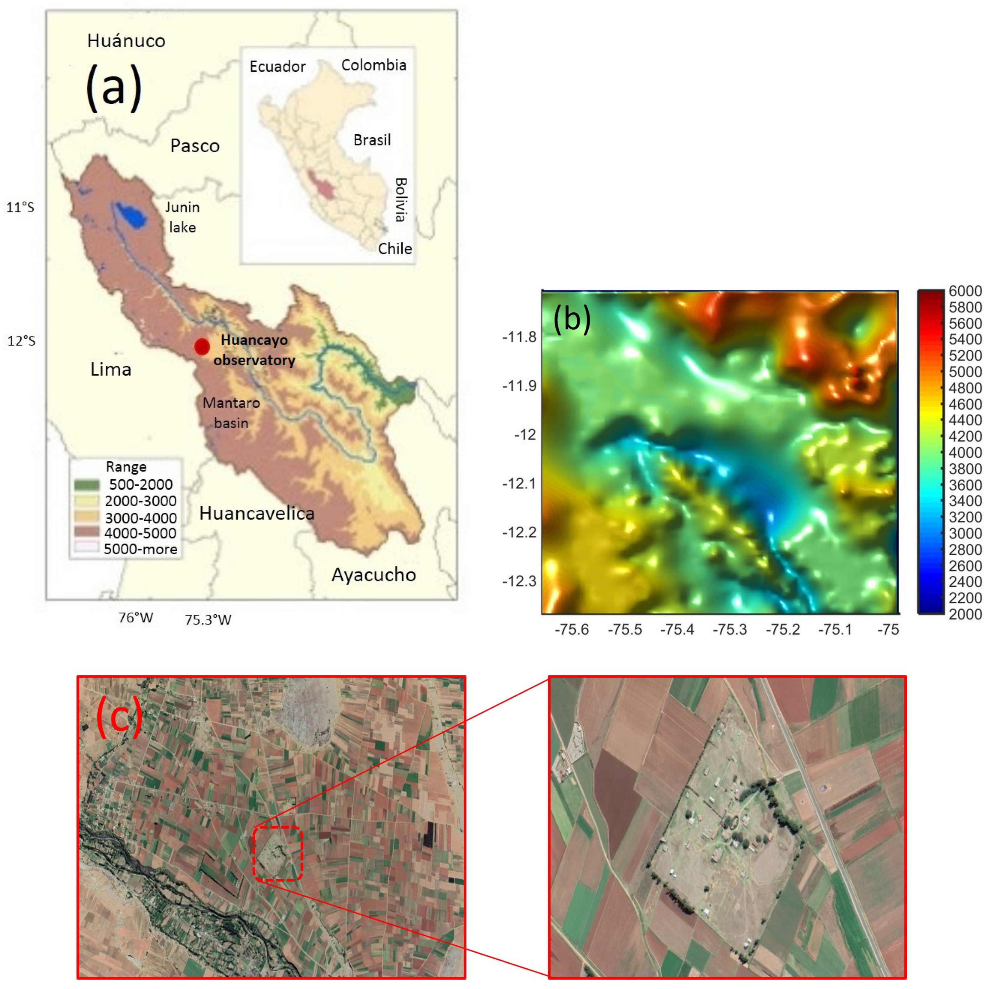
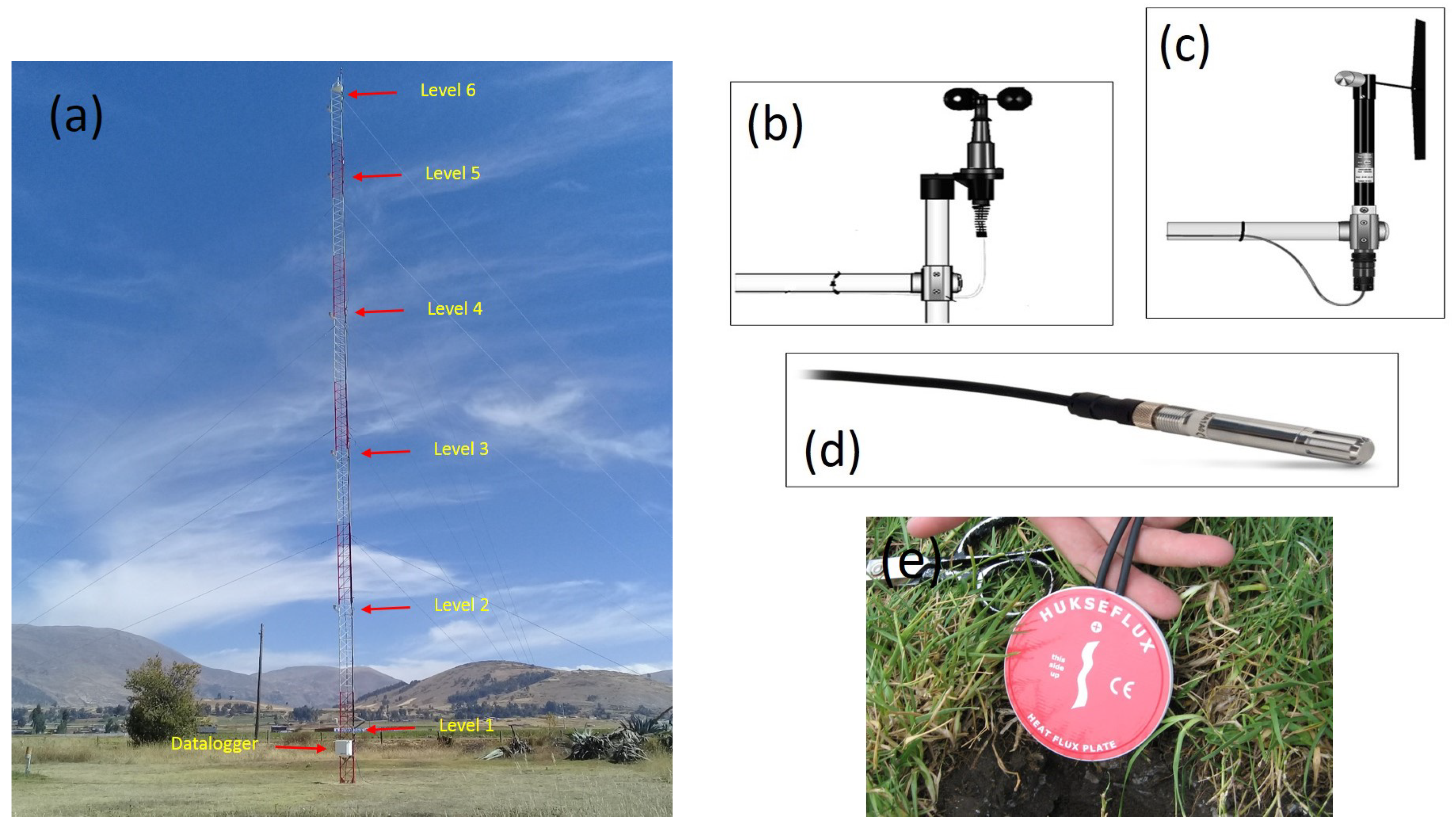
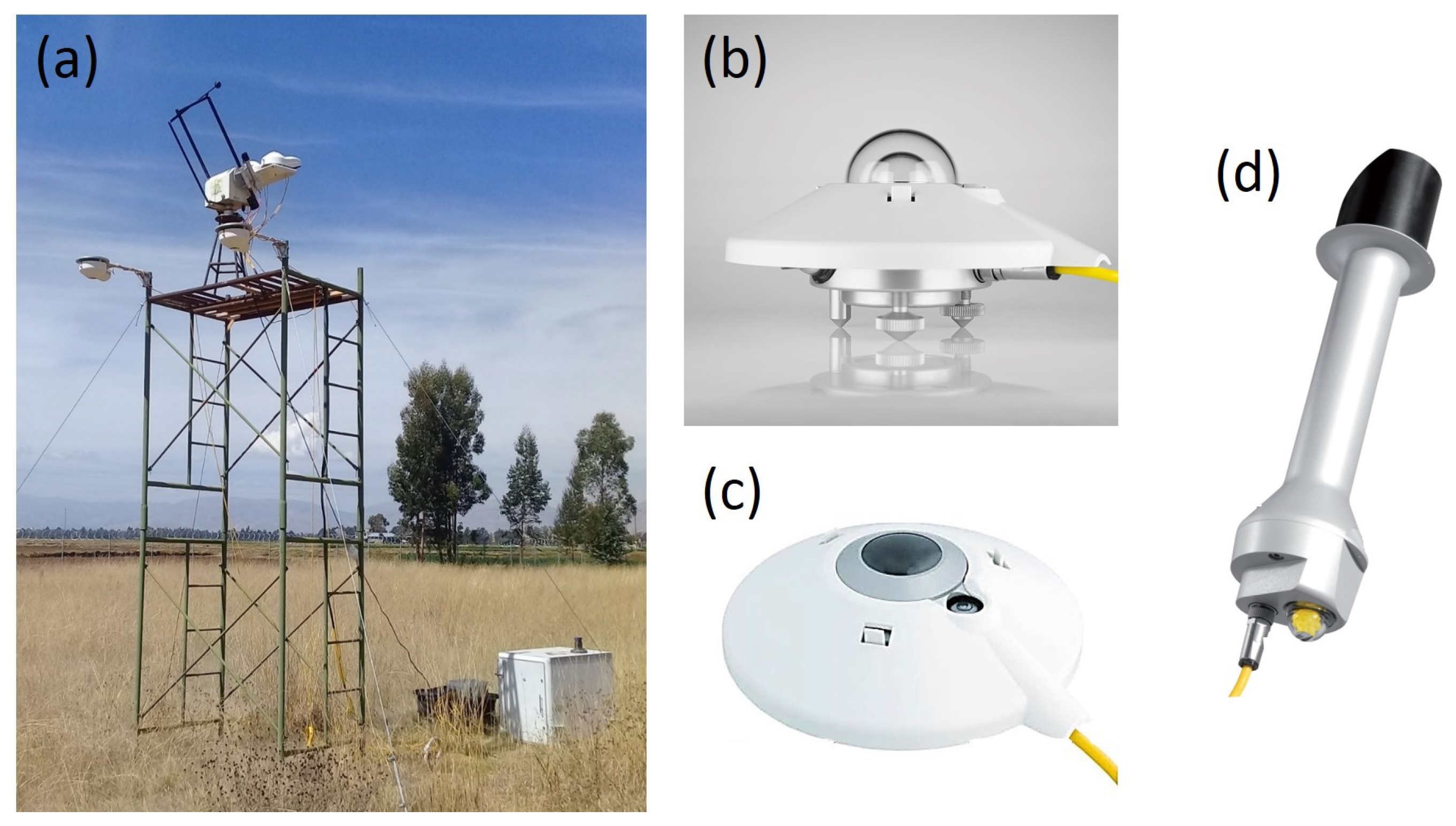
2. Site and Instrumentation

Measurements were made in the Huancayo observatory of the Geophysical Institute of Peru (12.05 S, 75.32 W, 3313 m asl) (Figure 1a) inside the Mantaro basin, which is located in the central Peruvian Andes (10 34 –13 35 S, 73 55 –76 40 W) with an area close to 34,550 km 2 . The altitudes of the Peruvian central Andes range from 500 to 5350 m asl and its average altitude is 3800 m asl (Figure 1b). The Mantaro Valley lies in the NW-SE direction and has a gentle slope of 0.2 . The climate information (1960–2002) measured at 07, 13 and 17 LT shows the Huancayo observatory has a marked seasonal variability in rainfall, with the maximum between January and March and the minimum between June to July. The mean accumulated rainfall during a year is 757.5 mm [29]. It was found that 83% of the annual rainfall takes place between October and April, 48% of which are distributed almost equally between January, February, and March. The maximum precipitation was found to be in February (120 mm) and the minimum in June (10 mm) [30].
The maximum mean temperatures have a less pronounced seasonality, with the highest value observed in November (20.8 C) and lowest in the wet months (February to March, 18.4 C). The minimum mean temperatures have a strong seasonality, ranging from its lowest values in the dry season (June to August), with its lowest in July (0.5 C), to its maximum values in the wet season (January to March) with an average value of 7 C [31]. The lowest values of the minimum mean temperature are associated with cloudless conditions with large outgoing long-wave radiation, mainly during the dry season [19]. The seasonal pattern of the rainfall is due to low cloud cover and specific humidity, with minimum values in June and July at 07 LT, which also coincides with the time of the minimum temperatures (between 06 and 07 LT) in the same months. Moreover, a low cloud cover presents higher values at 19 LT compared to the values at 07 and 13 LT, with maximum peaks of 6 oktas between January and February and minimum peaks below 3 oktas in the dry months for all observations. For specific humidity, diurnal variation is less pronounced with the minimum close to 5 g kg 1 at 07 LT in the dry months and maximums around 8.5 g kg 1 at 13 LT between January to March [19].
The sensors used to measure meteorological variables (temperature, relative humidity, wind speed, and wind direction) were installed in a gradient tower 30 m high (Figure 2a). Also, the measurements of solar irradiance components at the surface obtained by sensors installed in a radiometric tower 5 m high (Figure 3a) were used. The data of the sensors in the gradient tower were carried out regularly since May 2018, save the data of the radiometric tower since August 2017. All the data were recorded at a minute’s resolution. Temperature and relative humidity were measured by the HMP60 probe of Campbell Scientific (Figure 2d). The 03002 Wind Sentry Set of Campbell Scientific measures both wind speed and direction. It consists of a 3-cup anemometer and a wind vane mounted on a small crossarm (Figure 2b,c). Finally, the HFP01 soil heat flux plate (Figure 2e) sends out a voltage signal that is proportional to the heat flux of the surrounding medium (soil). To measure the soil temperature and moisture, Decagon 5TM VWC tensiometers were used. The 5TM delivers temperature, measured by an on-board thermistor, along with accurate volumetric water content. It can also determines determines volumetric water content (VWC) by measuring the dielectric constant of the soil using capacitance/frequency domain technology. All the details of these sensors are shown in Table 1.
The pyranometer CMP10 from Kipp & Zonen installed in the radiation tower (Figure 3b) is designated to measure the hemispherical (global or diffuse) SW irradiance. Three pyranometers CMP10 were installed, two to measure the SW global and diffuse irradiances incident at the surface and one to measure the SW irradiance reflected by the surface. To measure the diffuse irradiance from the sky, the direct solar irradiance is blocked by a small black sphere mounted on an articulated shading assembly in a two-axis automatic sun tracker, Kipp & Zonen 2AP. The sun tracker uses information on location and time to calculate the position of the sun and point at it accurately under all weather conditions (Figure 3a). The pirgeometer CGR4 from Kipp & Zonen installed in the radiation tower (Figure 3b) is designed to measure LW irradiance. The pyrheliometer CHP1 from Kipp & Zonen is designed to measure direct SW irradiance. All the details of radiative sensors are given in Table 2.

3. Methodology

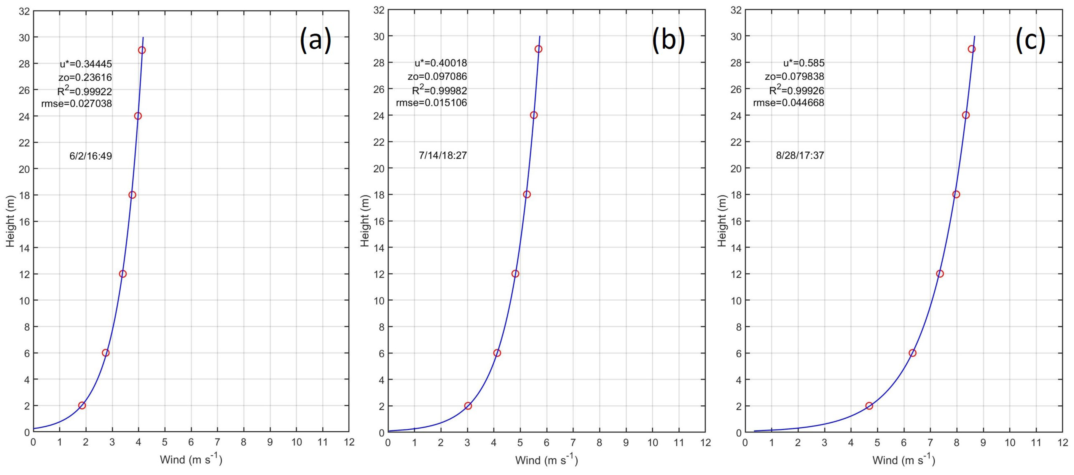
3.1. Roughness and Wind Variation

A logarithmic decay curve accurately describes the actual form of wind variation with height under neutral stability. The logarithmic wind profile equation is given by:
u ¯ z = u k · ln z z
where u ¯ z is the mean wind speed (m s 1 ) at the height z, u the friction velocity (m s 1 ), k is the Von Karman’s constant (∼0.40), and z the roughness length (m), which is a measure of the aerodynamic roughness of the surface and depends of the shape and density distribution of the elements. The surface shearing stress ( τ ) is the forced exerted on the surface by the air being dragged over it. It is function of u as follows:
u = τ ρ
where ρ is the air density. From Equation (2), it is possible to obtain τ , because u can be evaluated from wind profile measurements, using Equation (1). This method is limited to roughness elements with small vertical extension, as the bushes on the ground of the Huancayo observatory. The analysis of wind profiles and momentum flux during the observation period will be presented in Section 4.3.

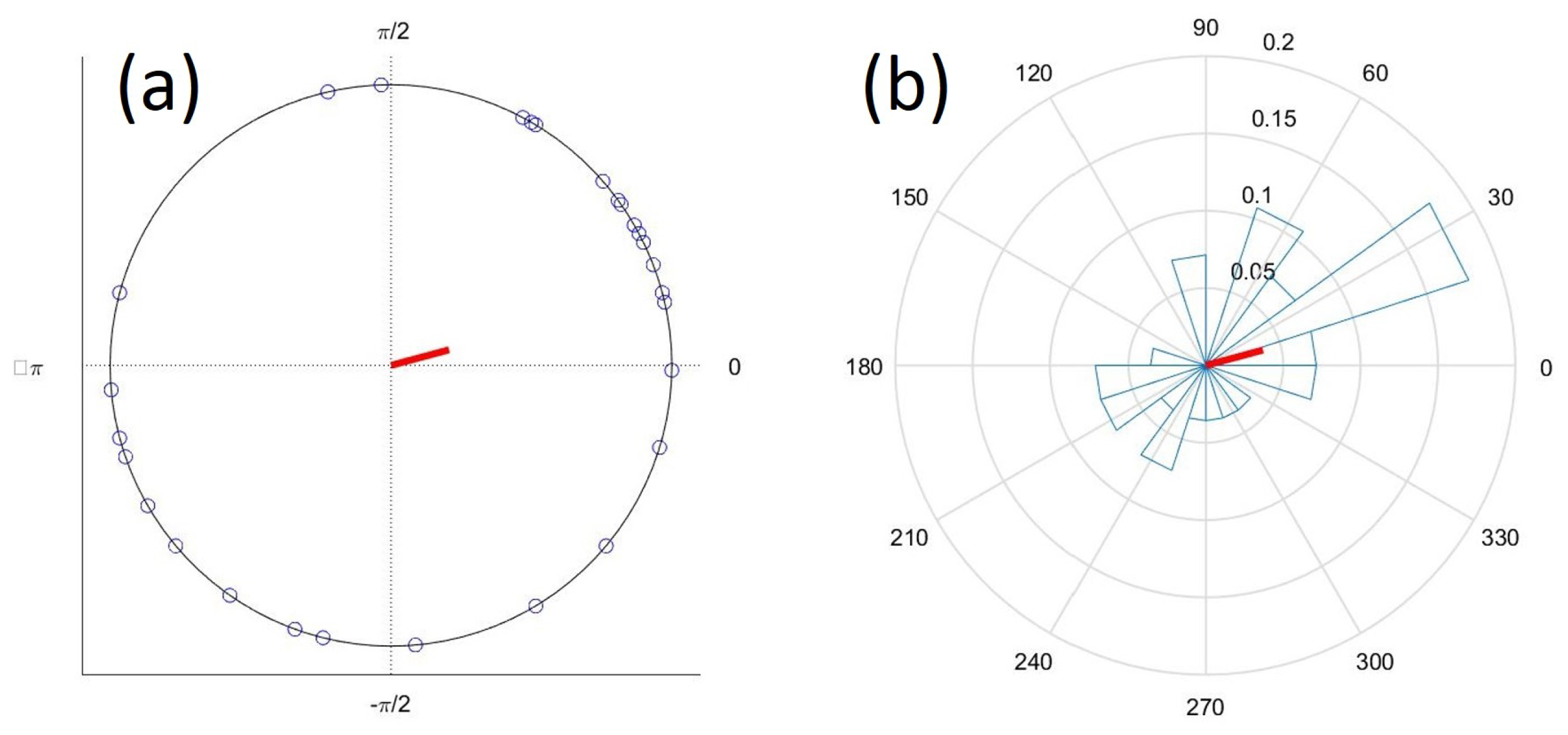
3.2. Wind Direction (Circular Statistics)

Wind direction angles have a circular nature and therefore such data cannot be analyzed with commonly used statistical techniques. To compute the mean and standard deviation of wind direction angles we used circular statistics, which is a set of statistical techniques for the use of data on an angular scale [32,33]. For instance, the mean of a sample of wind direction angles cannot be computed by simple averaging the data points, because angles close to zero and 360 deg have mean close to 180 deg, but this makes no sense and the correct mean value must be close to one of these two angles (0 or 360 deg.). Instead, directions are first transformed to unit vectors in the two-dimensional plane by:
r i = cos ( α i ) sin ( α i )
where r i is the unit vector and α i is the angle of the vector. This transformation is implemented using the Euler’s identity:
exp ( I α i ) = cos ( α i ) + I sin ( α i )
where I is the imaginary unit. After this transformation, the vectors r i are vector averaged by the following equation:
r ¯ = 1 N i r i
where r ¯ is called mean resultant vector, which is transformed using the four-quadrant inverse tangent function to obtain the mean angular direction α ¯ . For the present work we used the algorithms developed in two recent contributions [33,34]. As an example, Figure 4a shows a dataset consisting of 30 samples plotted as points on the unit circle and Figure 4b show angular histograms for the same dataset. The unit circle has limits from 0 to + π (counterclockwise) and from 0 to π (clockwise). In contrast the angular histograms shows the relative frequency of dataset and has limits from 0 to 360 deg (counterclockwise). In order to process the wind direction data, we made a transform of coordinates from cardinal directions to unit circle directions.

3.3. Estimation of Turbulent Energy Fluxes and Surface Albedo

For the present study, we used the flux–gradient methods which estimate the turbulent energy fluxes (sensible and latent) based on average profiles of atmospheric properties and the degree of turbulent activity. We measured air temperature, relative humidity, wind speed and wind direction in six levels of height with sensors located in a gradient tower (Figure 2) described in Section 2. There are two profile methods: the aerodynamic method [8] and the Bowen-ratio energy-balance method [35], which are based on the similarity principle proposed by Monin and Obukhov [6,36]. This holds that the diffusion coefficients and the aerodynamic resistance for momentum, heat, water vapor and carbon dioxide are equivalent. This condition means that a turbulent eddy can carry heat, vapor and momentum with equal efficiency. The Bulk Richardson number (Ri B ) is a non-dimensional stability parameter to characterize atmospheric stability and the state of the turbulence near the surface [7]. The Bulk Richardson number is a ratio that accounts for the effects of buoyancy and mechanical forgings (free to forced convection) and is expressed as:
Ri B = g T ¯ · Δ T ¯ / Δ z ( Δ u ¯ / Δ z ) 2
In this case, we assumed that the change of wind direction in low levels is very low, as can be seen in Section 4.3, and therefore can be ignored. In Equation (6), g is the acceleration due to gravity (m s 2 ), T ¯ (K) is the mean temperature in the layer Δ z (m), Δ T ¯ is the difference of the temperatures in the layer Δ z , Δ u ¯ is the difference of wind speed in the layer Δ z . Ri approaches zero for neutral stability conditions generally associated with early morning and/or evening periods on cloudy days with strong winds. Positive values of Ri indicate stable conditions where temperatures near the surface are cooler than away from the surface associated with early morning, evening night periods and overcast days. Negative values of Ri B indicate strong lapse rate (unstable) conditions where surface heating enhances buoyancy effects. In general, neutral conditions representing a minor fraction of a day with dominant unstable and stable conditions during the diurnal cycle [8]. The neutral form of the aerodynamic equations to estimate the turbulent energy fluxes of momentum ( τ ), sensible ( Q H ) and latent ( Q E ), can be generalized according to stability, as given by Ri B in the following operational equations, as described by Oke [7] and Arya [2]:
Q H = C a k 2 z 2 Δ u ¯ Δ z · Δ T ¯ Δ z · ( Φ M Φ H ) 1 Q E = L v k 2 z 2 Δ u ¯ Δ z · Δ ρ ¯ v Δ z · ( Φ M Φ V ) 1 τ = ρ k 2 z 2 Δ u ¯ ln ( z 2 / z 1 ) 2 · ( Φ M Φ V ) 1
where ρ v is the water vapor density, which was estimated used the relative humidity, the saturation vapor pressure and the air temperature. Moreover, C a is the heat capacity of air, L v is the latent heat of vaporization, k is the Von Karman’s constant (∼0.40), z is the log mean height (=( z 2 z 1 )/(ln( z 2 / z 1 )), Φ M , Φ H and Φ V are dimensionless stability functions for momentum, heat and water vapor, which can be expressed as functions of the Richardson number [2]:
Φ M 1 = ( 1 15 R i ) 1 / 4 for R i < 0 ( 1 5 R i ) for 0 < R i < 0.2 Φ X 1 = ( 1 15 R i ) 1 / 2 for R i < 0 ( 1 5 R i ) for 0 < R i < 0.2
where Φ X is the appropriate stability function for the property being transferred. Using these functions, it is possible to calculate the combined terms used in Equation (7):
( Φ M Φ X ) 1 = ( 1 15 R i ) 3 / 4 for R i < 0 ( Φ M Φ X ) 1 = ( 1 5 R i ) 2 for 0 < R i < 0.2
When the atmosphere is neutral (Ri between ±0.01) thermal effects are minimal and only forced convection is present. For conditions of higher instability, buoyancy effects grow in importance through the mixed regime. For values of Ri larger than −1.0, there is weak horizontal motion and strong convective instability. For positive values of Ri close to +0.25 the flow is laminar and vertical mixing is absent. Moreover, for the Bowen-ratio energy-balance method it is necessary to formulate a surface energy budget (SEB) equation for a surface or volume, applied to the interface between the atmosphere and the elements of the surface can be expressed as:
Q = Q H + Q E + Q G
where the net irradiance ( Q ) is the main source (or sink) of energy during daytime (night-time) and drive the sensible ( Q H ) and latent ( Q E ) turbulent heat fluxes and the energy of conduction to or from the underlying soil ( Q G ). The Bowen-ratio energy-balance method estimates the convective fluxes by computing the available energy ( Q Q G ). This available energy is partitioned between Q H and Q E by considering their ratio, ( β ), given by:
β = Q H Q E = C a Δ T ¯ L v Δ ρ ¯ v
From the surface energy-balance equation (Equation 10), the individual turbulent fluxes are given in terms of β as:
Q H = β ( Q Q G ) ( 1 + β )
Q E = ( Q Q G ) ( 1 + β )
This method has the advantage of not being stability-limited because it only requires similarity between Φ M , Φ H and Φ V . We used only measurements with a difference of the wind velocities between both heights greater than 0.3 m s 1 to ensure that a sufficient turbulent regime exists [37]. Also, Bowen ratio values close to −1 were rejected to eliminate unacceptable results [38]. To replace missing data, we used data from the preceding and succeeding period for interpolation [39]. Several studies applied the Bowen-ratio technique to estimate the turbulent fluxes in different types of regions [40,41,42,43]. However, there are some problems when the gradient of the specific humidity is very small, which generates errors in the estimation of latent heat flux [10].
The most important disadvantage of the Bowen-ratio method is that because of the apparent unclosed energy balance, the residual or imbalance (Imb) is either added to the net radiation or distributed according to the Bowen ratio to the sensible and latent heat flux. This assumption could generate important uncertainties [18,44]. The Imb term is an unavoidable part of the experimentally determined surface energy budget, and it is usually between 10–15% in wide homogeneous conditions (as during the EBEX campaign, [45]) increasing as the terrain becomes more heterogeneous (as for LITFASS-2003 [46]) or topographically complex to 20–35% [15,16]. For both methods (aerodynamic and Bowen ratio), we used differences of wind, temperature and moisture at six levels of height, taking differences between measurements of the sensors located at highest levels (6 m, 12 m, 18 m, 24 m and 29 m) and the lowest level (2 m) of the gradient tower (Figure 2). Also, we used moving averaging periods of 30 min which are considered appropriated [7,47]. The analysis of air temperature, moisture and turbulent and radiative energy fluxes during the observation period will be presented in Section 4.
It is important to note that despite the widely used SEB equation (Equation 10), there are more processes that modify the energy of the volume and are customarily neglected. These terms include transient conditions such as morning or evening transitions ( T T ), advection of heat due to local heterogeneities (A), storage in the elements of the volume (S), biological processes (B) and instrumental errors (O t ) [17,48,49]. These terms can be grouped in the imbalance (Imb) term as follows [18]:
Q Q H Q E Q G = T T A + S + B + O t = Imb
The absorption or release of heat by the air, soil and plant biomass generates the physical storage changes of the volume (S). Changes of sensible heat content (but not of latent heat changes) result in temperature. the rate of CO 2 assimilation by the plants generates changes in biochemical energy storage (B). The analysis of the components of the SEB and the imbalance term during the observation period will be presented in Section 5.5.
Moreover, the surface albedo is another magnitude that characterizes the interaction of solar radiation with the earth’s surface. The study of this variable allows us to establish the relationship between the amount of irradiance reflected by the surface, with respect to the amount of indistinct global irradiance [50]. The surface albedo depends on the surface properties, as well as its conditions such as color, moisture, presence or lack of vegetation, roughness, etc. For tropical regions climatology surface albedo (30 years) was estimated between 0.19 and 0.26 [51] by using a dataset subjected to a quality control following the criteria of the Baseline Surface Radiation Network (BSRN) and with the methodology of the WMO Guide to Climatological practices [52]. The analysis of the surface albedo obtained for the Mantaro valley will be presented in Section 4.5.

3.4. Land Surface Temperature

The irradiance measured ( L m s ) by the LW irradiance sensor (Figure 3c) looking downwards to the surface is the sum of LW irradiance emitted by the surface ( L u p ) plus the LW irradiance product of the reflection of the downward LW coming from the sky ( L d n ) [53]. For an opaque surface with LW emissivity ( ϵ ), L m s is equal to:
L m s = L u p + ( 1 ϵ ) L d n
Considered that L u p = ϵ σ LST 4 , where LST is the land surface temperature and σ is the Stefan- Boltzmann constant ( σ = 5.67 × 10 8 W m 2 K 4 ) and we used a value of 0.97 for ϵ as was recommended in previous studies for organic bare soil [53,54], then LST can be expressed as:
L S T 4 = L m s ( 1 ϵ ) L d n ϵ σ
Taking into account the general formula of error propagation the uncertainty of LST is between 3 and 4 K for an LST close to 300 K. The analysis of land surface temperature is presented in Section 4.5.

3.5. Ground Heat Flux at the Surface

During the day, the ground surface and the canopy is heated by incoming short-wave irradiance. In contrast, at night hours the emission of long-wave up-welling irradiance causes the cooling of the surface, which becomes cooler than the air and the deeper soil layers. The available energy according to the net all-wave radiation ( Q ) is distributed by the turbulent sensible ( Q H ) and latent ( Q E ) heat fluxes and the mainly molecular ground heat flux ( Q G ) which is based mainly on molecular heat transfer and is proportional to the temperature gradient ( T / z ) times the thermal molecular conductivity a G (W m 1 K 1 ). To estimate the ground heat flux at the surface we used the sum of the soil heat flux measured at 8 cm by a soil heat flux plate (Figure 2e) and the heat storage in the layer between the surface and the plate [44]:
Q G ( 0 ) = Q G ( 8 c m ) + z 0 C G ( z ) T ( z ) d z
where C G is the volumetric heat capacity C G (z) = a G / ν T ( ν T is the molecular thermal diffusivity) that can be assumed constant with depth in the case of uniform soil moisture. To implement Equation (17) we used two integrating temperature sensors of the soil layer, which are located at 2 cm and 5 cm between the surface and the heat flux plate (8.0 cm). For the ground heat flux near the surface, it follows that:
Q G ( 0 ) = Q G ( 8 c m ) + C G | Δ z | | T ( t 2 ) T ( t 1 ) | t 2 t 1
In addition, C G of moist soil at different soil levels were calculated by adding the heat capacity of the dry soil to that of the soil water as follows:
C G = C d + θ V ρ W C W
where C d is the heat capacity of dry soil, θ V is the soil water content on a volume basis, ρ W is the density of water (1000 kg m 3 ) and C W is the specific heat of water (4.18 × 10 3 J kg 1 K 1 ). A value of 1.25 × 10 6 J m 3 K 1 for the heat capacity of dry soil is a reasonable value for a clay soil according to the soil characteristics of the Huancayo Observatory [55]. The analysis of soil temperatures, soil moistures and ground heat fluxes during the observation period is presented in Section 4.4 and Section 4.6, respectively.

4. Results

This section presents the results and discussions of the seasonal and diurnal cycles behavior of the surface boundary layer and of the energy-balance components between May 2018 and April 2019. Table 3, Table 4 and Table 5 show the mean monthly values of meteorological (at 2 m and 29 m), radiative and energetic variables, respectively.

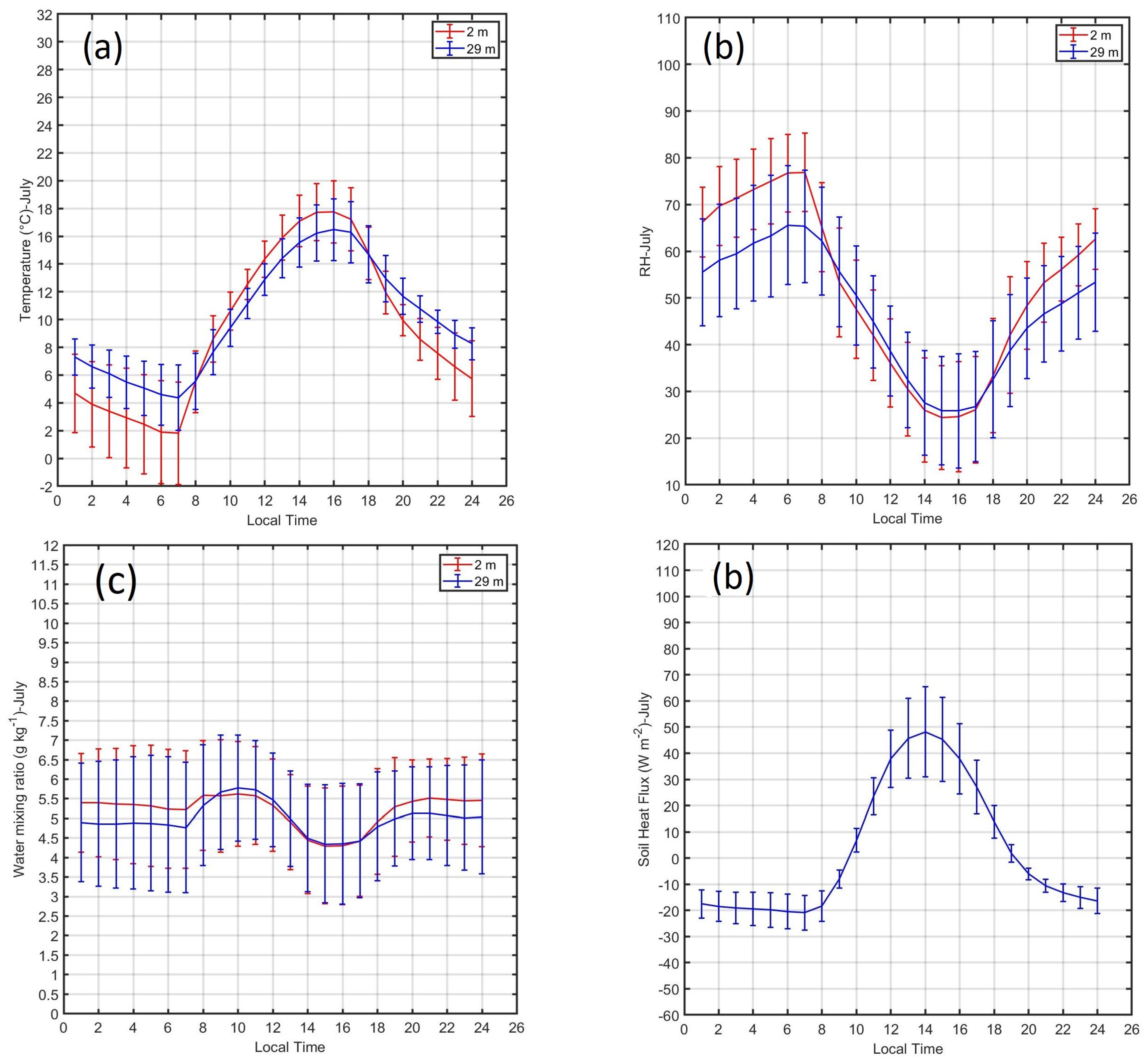
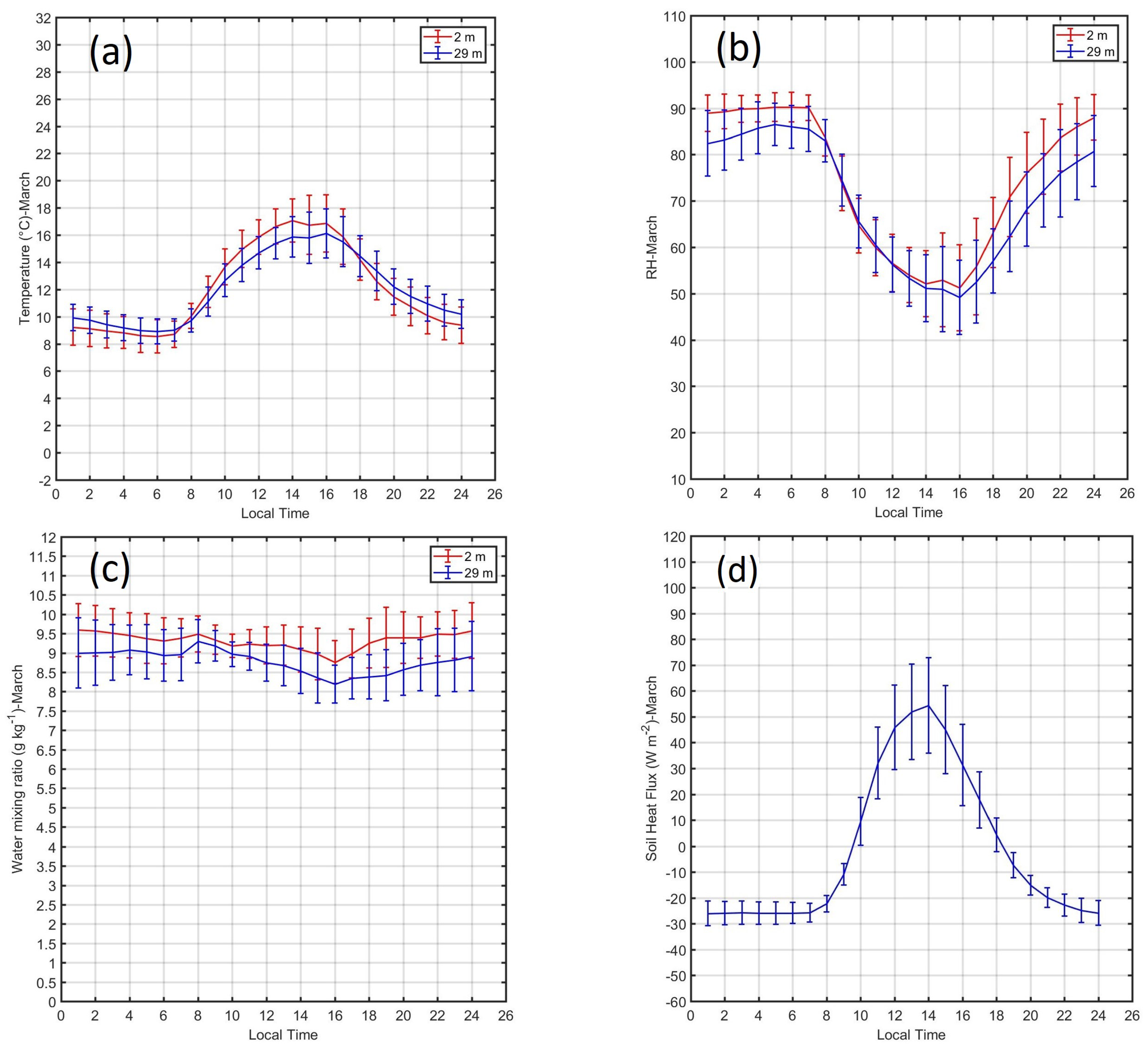
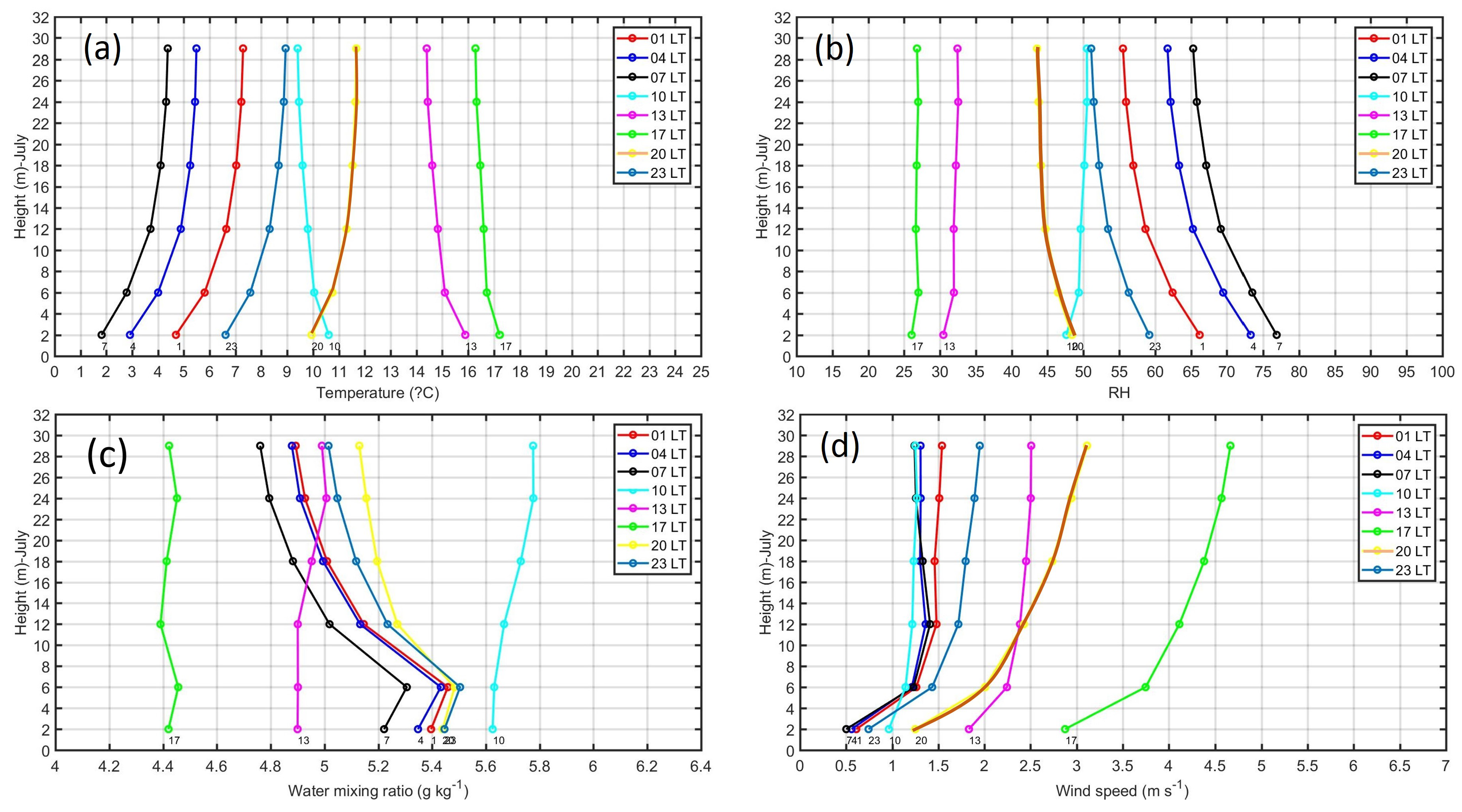
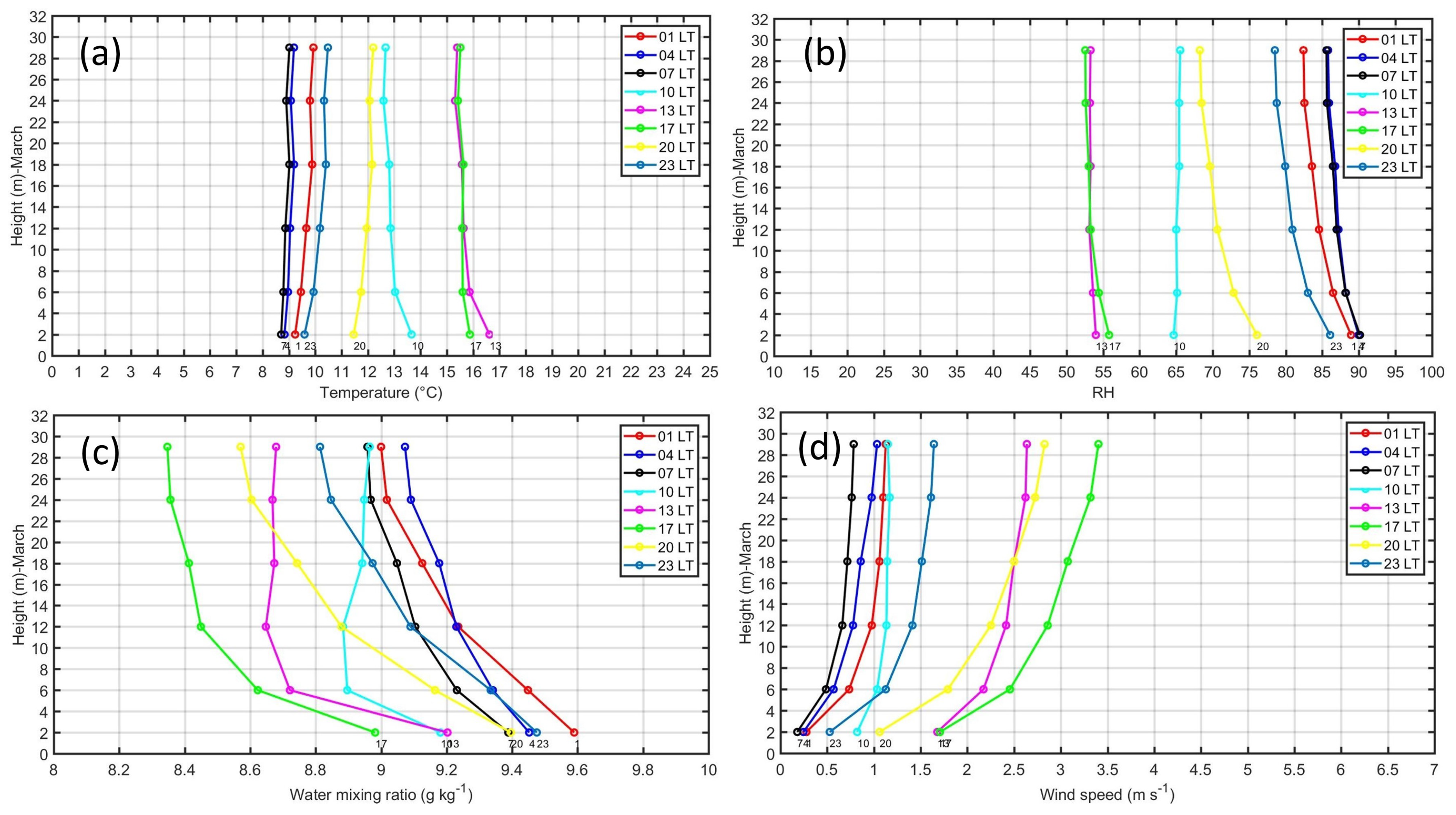
4.1. Air Temperature

The diurnal cycle of the mean monthly air temperatures during July (Figure 5a) and March (Figure 6a) showed the continuous decrease of temperature at night hours until reaching its minimum at 07 LT (Table 3-columns 2 and 3). During these hours, minimum temperature was observed during July at 07 LT (1.81 C at 2 m) and the maximum in March at 07 LT (8.71 C at 2 m). After sunrise the temperature increased between 18 C and 20 C around 16 LT for all months, reflecting the diurnal lag between maximum temperature and maximum solar irradiance (noon). During the night, between 18 LT and 8 LT, the temperatures were lower near the surface (2 m) than at 29 m by about 4 C in July and 0.5 C in March. However, at day hours the opposite occurred with differences close to 2 C for all months.
The diurnal cycle of temperature vertical profiles during July (Figure 7a) and March (Figure 8a) showed that most stable atmospheres were observed at night hours in July with positive lapse rates close to +0.25 C m 1 but in March the atmosphere remained slightly unstable or neutral with lapse rates close to 0 at night hours. At 10, 13 and 17 LT were observed unstable conditions with negative lapse rates between −0.13 and −0.25 C m 1 which was higher than the dry adiabatic lapse rate (−9.8 × 10 3 C m 1 ). After sunset (20 LT), the atmosphere became stable again with positive environmental lapse rates around +0.20 C m 1 .

4.2. Air Moisture

The diurnal cycle of RH during July (Figure 5b) and March (Figure 6b) showed the continuous increase of RH during the night until reaching their maximum values at 07 LT with 76.88% (65.0%) at 2 m (29 m) in July and almost constant values close to 90% (85%) at 2 m (29 m) in March. (Table 3-columns 4 and 5). After sunrise RH decreases up to 25% in July and 50% in March around 16 LT according to the time of maximum temperature. In the late afternoon the RH increased again according to the decrease of temperature (Figure 5a and Figure 6a) and the increase of water vapor (Figure 5c and Figure 6c). At day hours, between 8 LT and 18 LT, the RH was slightly higher at the highest level (29 m) in comparison with the RH near the surface (2 m) by about 2% and at night hours the opposite happens, with higher differences of RH between both levels by about 10%.
The diurnal cycle of vertical profiles for RH during July (Figure 7b) and March (Figure 8b) showed that at night hours, the RH decrease with high according to the inverted vertical profiles of temperature. However, during the day, the RH profiles remain almost constant probably as a consequence of high values of water mixing ratios (Figure 6c) and low stratification of temperatures (Figure 6a) along the day.
The diurnal cycle of the water mixing ratio during July (Figure 5c) and March (Figure 6c) showed a slight decrease during early morning hours close to 5.4 g kg 1 at 2 m in July and remains almost constant with values close to 9.5 g kg 1 in March (Table 3-columns 6 and 7). In July, after sunrise water mixing ratio increased up to 5.5 g kg 1 at 10 LT and by 11 LT decreases slightly until reaching its minimum close to 4.0 g kg 1 at 15 LT and around 17 LT increases again up to values around 5.5 g kg 1 . In March, decreases slightly until reaching its minimum value close to 8.70 g kg 1 at 16 LT. The differences between moisture content between 2 and 29 m is higher in March than in July.
The diurnal cycle of vertical profiles for water mixing ratio during July (Figure 7c showed that at night hours and early morning hours, were observed that the water vapor profiles become inverted near the surface (below 6 m). At day hours, the water vapor remains almost constant with a slightly inversion from 12 m up to 29 m. The vertical profiles of water mixing ratio along the day during March (Figure 8c showed high negative slopes for all hours because of the transfer of moisture from the surface to the atmosphere. The negative slopes were higher at afternoon hours (13–17 LT) and lower at early morning hours (01 LT–07 LT).

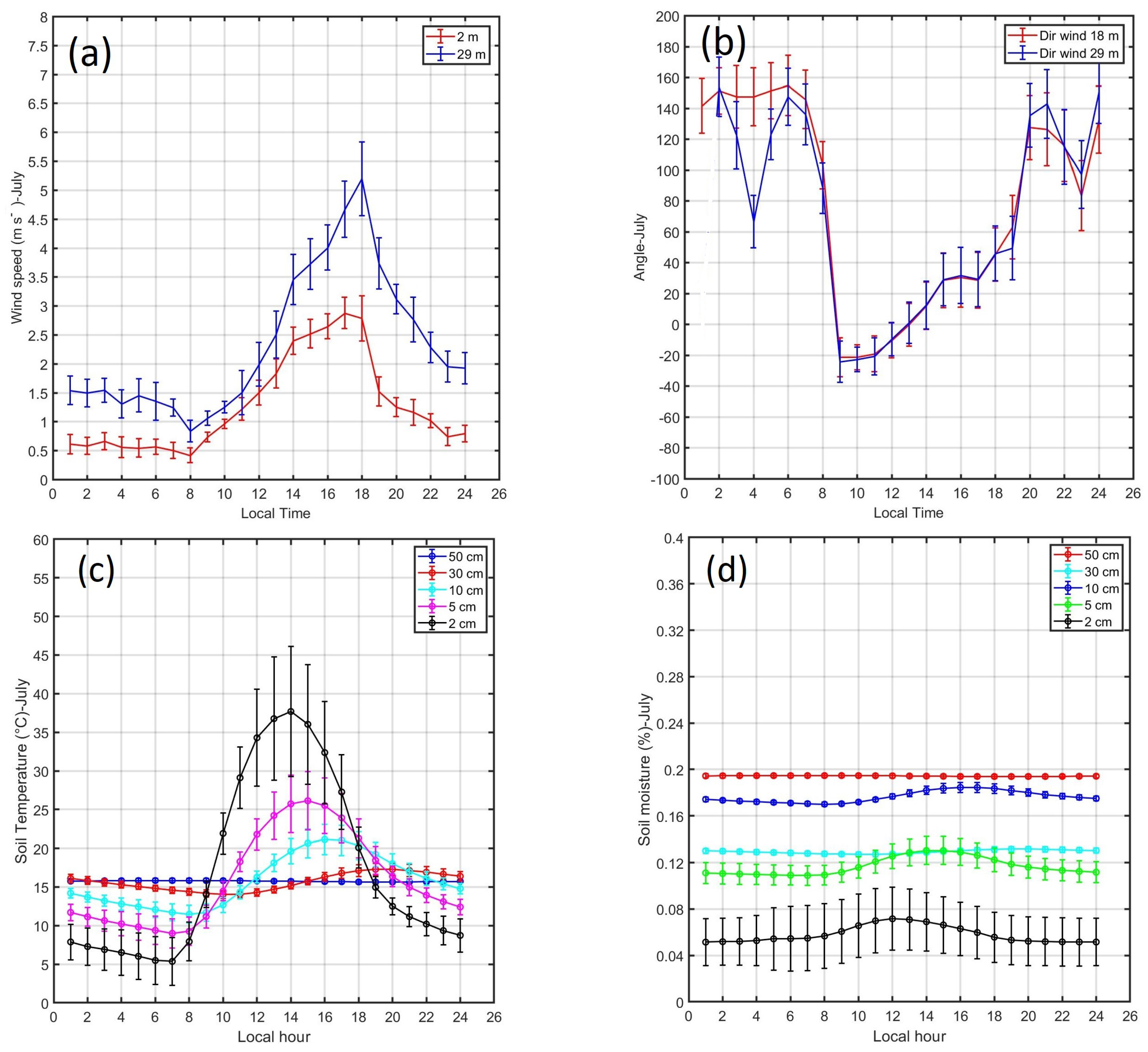
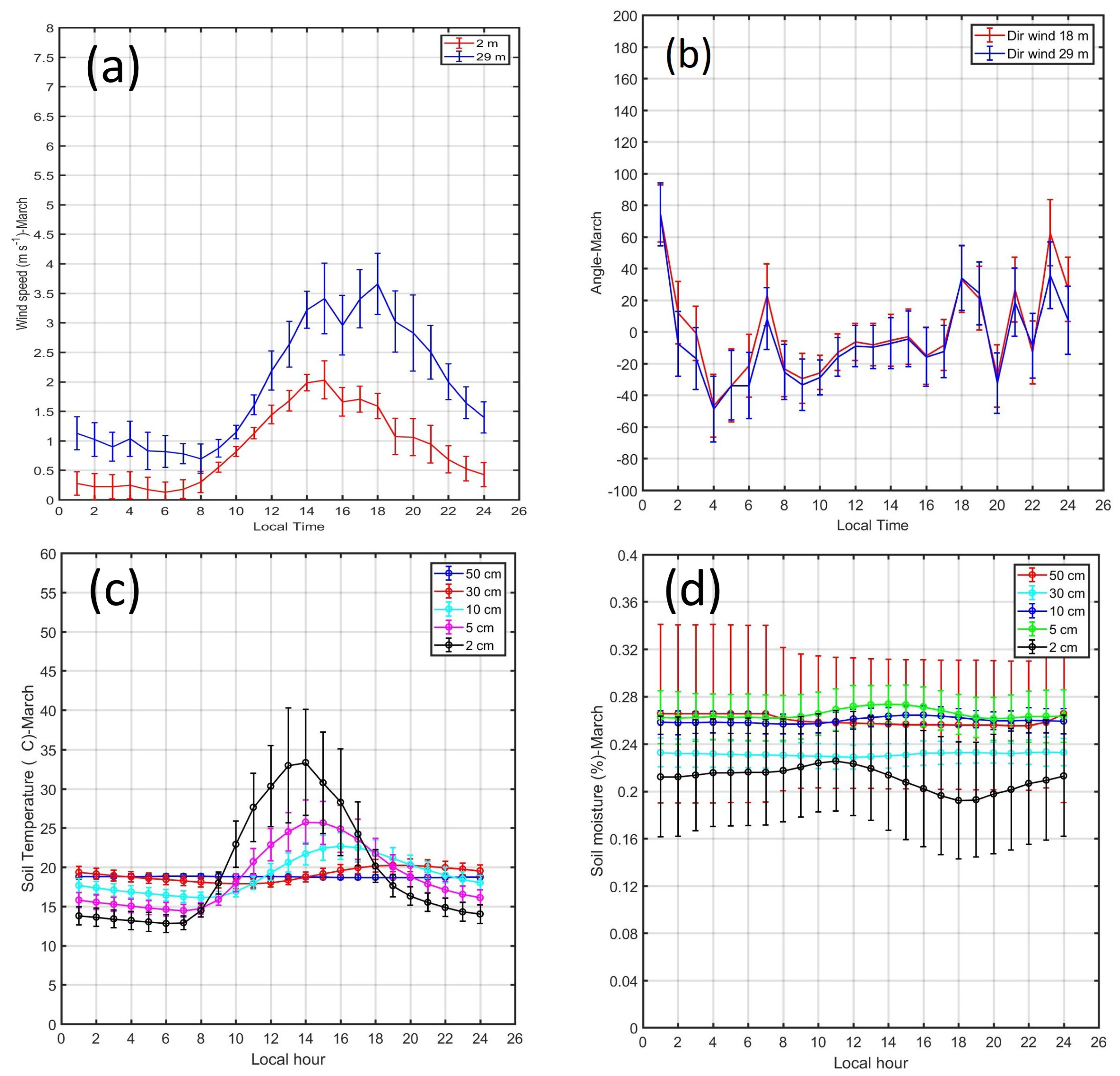
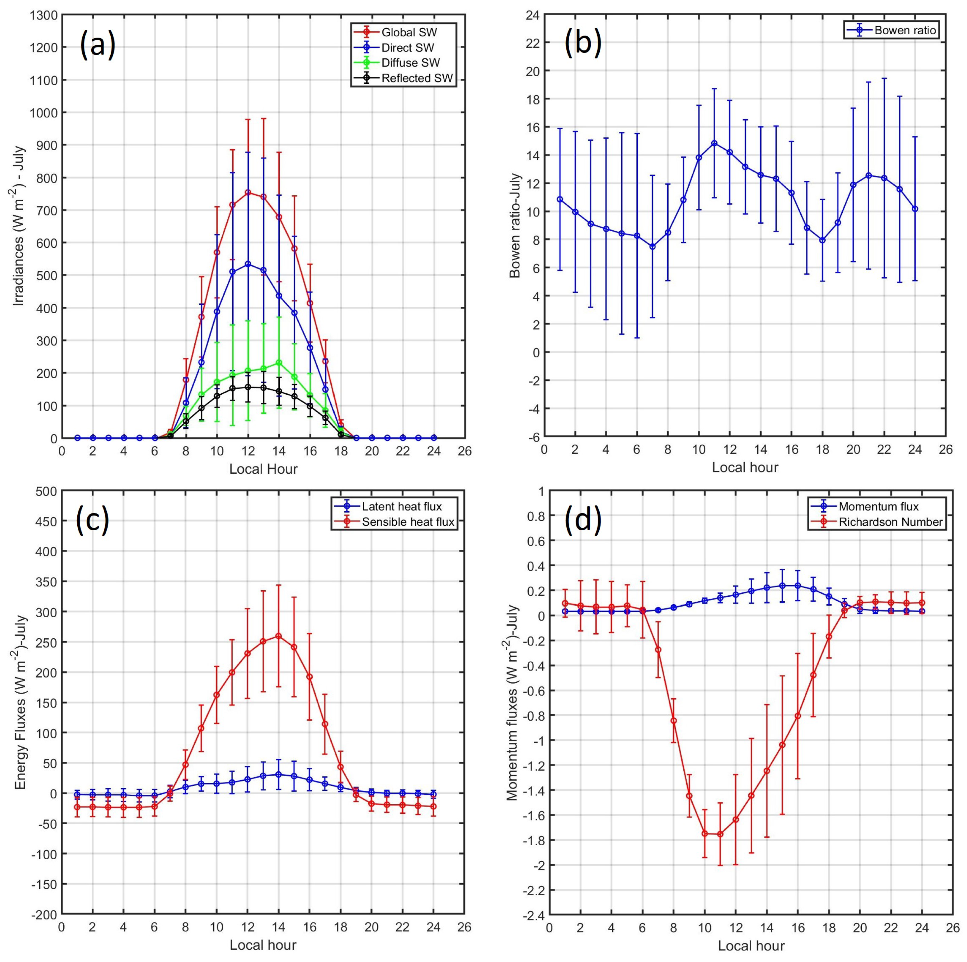
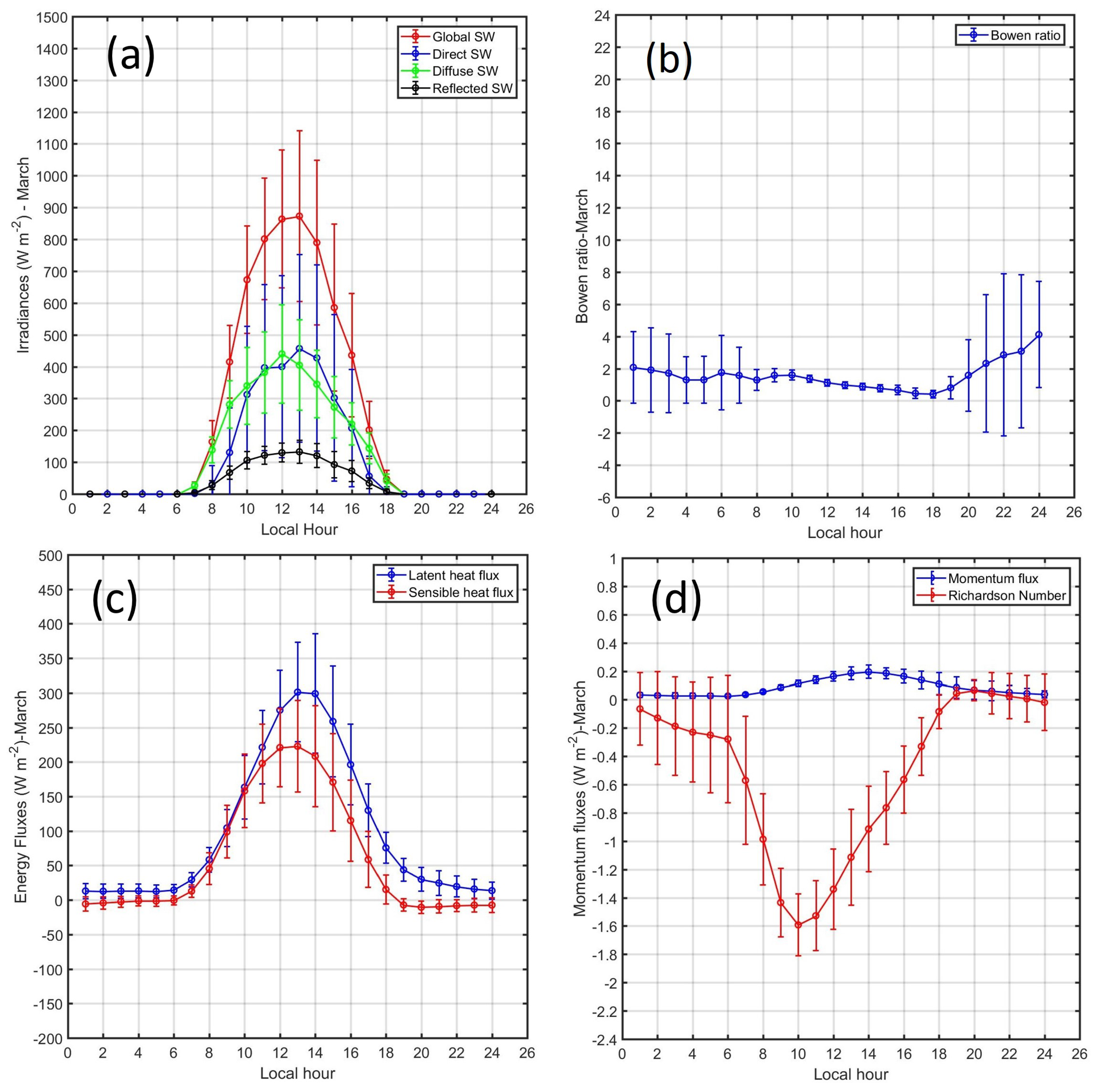
4.3. Wind Profiles and Momentum Flux

Figure 9a shows the diurnal cycle of wind speed during July. The minimums were observed between 07 and 08 LT close to 0.5 m s 1 (1.0 m s 1 ) at 2.0 m (29.0 m) and the maximums were observed around 18 LT close to 3.0 m s 1 (5.0 m s 1 ) at 2.0 m (29.0 m) (Table 3-columns 8 and 9). In contrast, the diurnal cycle of wind speed during March (Figure 10a) showed minimum at 06 LT close to 0.2 m s 1 (0.9 m s 1 ) at 2 m (29 m) and the maximums were observed around 15 LT close to 2.0 m s 1 (3.5 m s 1 ) at 2.0 m (29.0 m).
The diurnal cycle of wind speed vertical profiles during July (Figure 7d) and March (Figure 8d) showed the well-known almost logarithmic decay curve with low vertical gradients for all hours and higher gradients and intensities at day hours. The maximums were observed at 17 LT close to 3 m s 1 (4.6 m s 1 ) at 2 m (29 m) in July and close to 0.2 m s 1 (0.8 m s 1 ) at 2 m (29 m) in March. The minimums were observed at 07 LT close to 0.5 m s 1 (1.3 m s 1 ) at 2 m (29 m) in July and close to 0.2 m s 1 (0.8 m s 1 ) at 2 m (29 m) in March.
The diurnal cycle of wind direction during July (Figure 9b) showed that during night and early morning hours, the wind direction coming from the west and north-west (60 to 160 ) (Table 3-column 10) and during the day from the north-east and south east ( 20 to 60 ). This change of the wind direction along the day was associated with the mountain–valley circulation (Figure 1b). The diurnal cycle of wind direction during March (Figure 10b) showed a similar behavior but with lower amplitude and angles varying from 50 to 80 .
Roughness length ( z ) is a measure of the aerodynamic roughness of the surface and depends on wind speed. In order to estimate z for the natural surface in the Huancayo observatory for the period between May 2018–April 2019, we selected wind profiles under neutral conditions that fit with the logarithmic equation shown in Equation (2) (Ri∼0) with a coefficient of determination (R 2 ) higher than 0.99 and root mean square deviation (RMSE) lower than 0.05.
For instance, Figure 11 show the wind speed profile for three different times. The first z is 0.24 at 1649 LT, the second z is 0.1 at 1827 LT and the third is 0.8 at 1737 LT. For these cases it was observed that the wind speed reach values between 4 and 7 m s 1 at 29 m high. Using the conditions mentioned above we found 413 wind profiles that may be consider near neutral. It was estimated the median of z close to 0.20 m, with percentile 75% close to 0.42 and percentile 25% close to 0.11 (Equation (2)). For the friction velocity ( u ). Moreover, we estimated the median close to 0.29 m s 1 , with percentile 75% close to 0.39 m s 1 and percentile 25% close to 0.22 m s 1 .

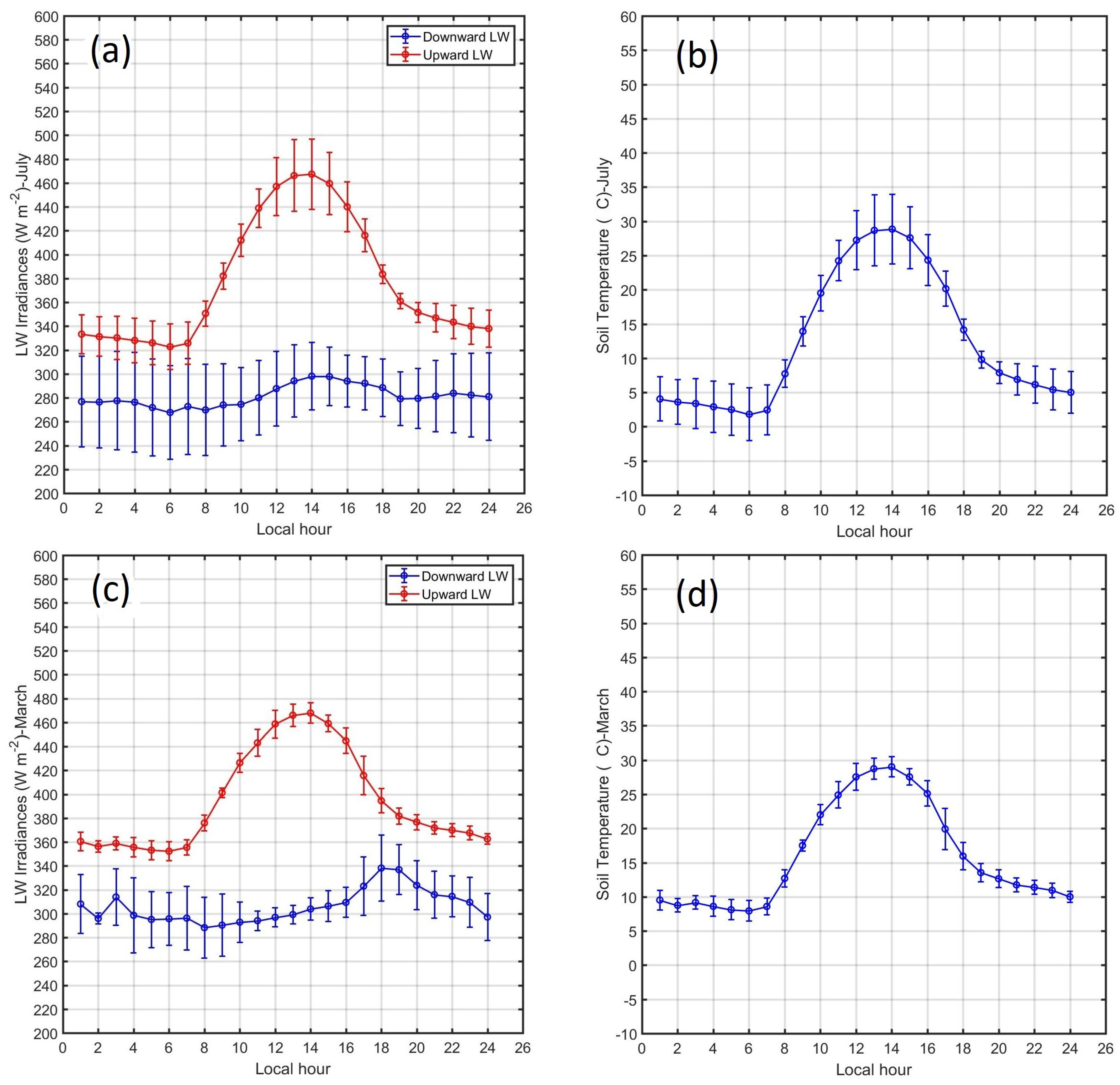
4.4. Soil Temperature and Soil Moisture

The diurnal cycle of the mean monthly soil temperatures at 2, 5, 10, 30 and 50 cm depth during July (Figure 9c) showed that the near surface temperature (2 cm depth) variation is wave-like with minimum close to 5 C at 07 LT (Table 4-column 8) and maximum close to 38 C at 14 LT in July and with minimum close to 13 C at 06 LT and maximum close to 33 C at 14 LT in March. For the other depths, the soil temperature amplitudes were decreasing and the times of maximum and minimum temperature were lagged (shift to the right in time). At 50 cm the soil temperature is almost constant during the entire day with a value close to 15 C in July and to to 20 C in March.
The diurnal cycle of the mean monthly soil moisture at 2, 5, 10, 30 and 50 cm depth during July (Figure 9d) and March (Figure 10d) showed that the behavior of the near surface moisture (2 cm depth) was similar to the soil temperature (wave-like variation) with minimums close to 5% at night and early morning hours (Table 4-column 9) and maximums close to 7% at noon. For the other depths, the moisture amplitudes were decreasing and the times of maximum and minimum temperature were lagged (shift to the right in time). In July, at 50 cm the soil moisture was almost constant during the entire day with a value close to 20%. In contrast, in March the soil moisture showed close values between 20% at 2 cm depth and 25% for the other depths.

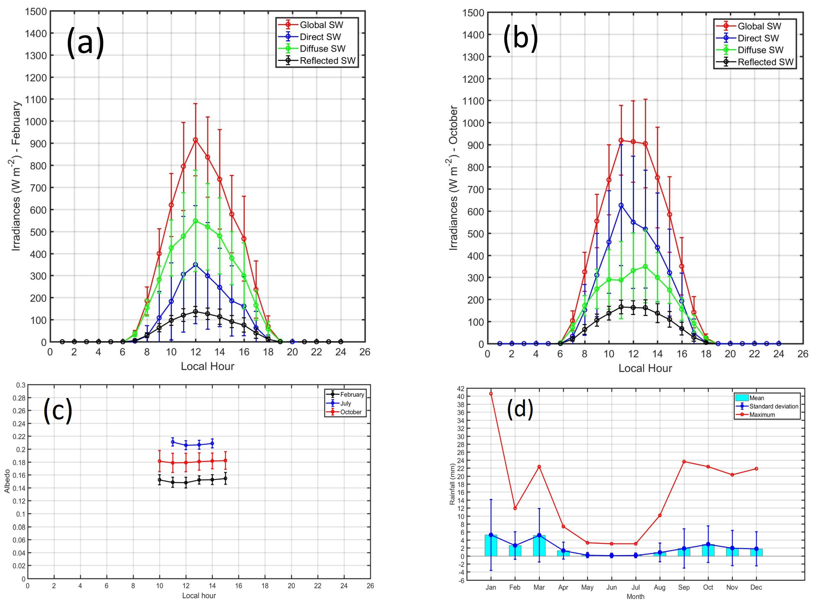
4.5. Land Surface Temperatures and Albedo

The diurnal cycle of mean monthly LST (Section 3.4) for July (Figure 12b) and March (Figure 12d) showed minimum LST values close to 2.5 C (9.78 C) at 06 LT in July (March) and maximum close to 29 C at 14 LT for both months. The diurnal thermal amplitude of soil was greater in July than in March. In July during night hours the difference between the air temperature at 2 m (T2) (Figure 5a) and LST was positive (the air is warmer than LST) between 0 C and 1.0 C but during day hours this difference (T2-LST) reached negative values between 1.5 C at early morning and 11 C around noon. In contrast, in March during night hours the difference between the air temperature at 2 m (T2) (Figure 6a) and LST was negative (LST is warmer than the air) around 1.4 C and during day hours this difference (T2-LST) became more negative with values between −1.5 C at early morning and −12 C around noon.
On the other hand, the diurnal cycle of surface albedo between 10 LT and 15 LT during February, July and October are shown in Figure 13c. In February, the surface albedo had values around 0.15, in July around 0.21 and in October close to 0.18. The surface albedo is a measure of how much SW irradiance that hits a surface is reflected without being absorbed. Therefore, the seasonal cycle of mean monthly SW irradiances during March (Figure 13a) and October (Figure 13b) explain the seasonal cycle of the surface albedo.
In March, the Global SW irradiance reached maximum close to 890 W m 2 at noon and the reflected SW irradiance reached maximum close to 120 W m 2 . But in October the Global SW irradiance reached maximum values close to 910 W m 2 at noon and the reflected SW irradiance has maximum values close to 180 W m 2 . Moreover, in July the Global SW irradiance reached maximum close to 750 W m 2 at noon but the reflected SW irradiance had maximum close to 160 W m 2 which increased the value of surface albedo up to 0.21.
The surface albedo also depends on the state of the soil and vegetation which are functions of the amount of moisture and precipitation. Figure 13d shows the mean monthly and maximum daily accumulated precipitation during 2018. A well-defined seasonal cycle with maximum precipitation was observed between January and March (summer) and minimum between June and August (winter) with significant rainfall between September and December (spring). The maximum mean (maximum) daily accumulated precipitation occurred in January with a value close to 5 mm (40 mm) and the minimum occurred in June with a value close to 0 mm (3 mm).

4.6. Energy Fluxes and Stability

The diurnal cycle of mean monthly turbulent energy fluxes ( Q H and Q E ) during July (Figure 14c) shows that at day hours was observed an important predominance of Q H with values close to 250 W m 2 in comparison with Q E with values around 30 W m 2 at 14 LT. At night and early morning hours (Table 4-column 2 and 3), Q H presents negative values close to −25 W m 2 and Q E close to zero with slightly negative values from 01 LT to 06 LT. In contrast, at day hours during March (Figure 15c) was observed a predominance of Q E with values around 300 W m 2 in comparison with Q H with values around 230 W m 2 at 13 LT. However, at night hours and early morning hours (Table 4-column 2 and 3), Q H presented slightly negative values around −5 W m 2 and Q E presented positive values around +15 W m 2 from 01 LT to 6 LT.
The diurnal cycle of momentum flux during July (Figure 14d) shows that the maximum value is close to 0.2 N m 2 at 15–16 LT. A similar pattern was observed for the momentum flux during March (Figure 15d) but with maximum around 14 LT and minimum between 0.036 N m 2 and 0.050 N m 2 at early morning hours (Table 4-column 4).
Moreover, the diurnal cycle of mean monthly Ri during July (Figure 14d) shows that at day hours were observed negative values with minimum close to −1.8 at 10 LT and during the night were observed positive values with maximum close to 0.1 at night and early morning hours (Table 4-column 5). In contrast, the diurnal cycle of mean monthly Ri during March (Figure 15d) shows positive values only after sunset until 20 LT, next Ri becomes negative up to −0.2 at sunrise.
The diurnal cycle of mean monthly β during July (Figure 14b) showed high values around 8 with two maximums of 14 at 1100 LT and 12 at 2100 LT. In contrast, the diurnal cycle of mean monthly β during March (Figure 15b) shows low values with minimum close to 0 at 18 LT and maximum around 4 at 0 LT (Table 4-column 6).
The diurnal cycle of mean monthly soil heat flux (8 cm depth) during March (Figure 6d) shows negative values between −8 W m 2 at 19 LT and −25 W m 2 at early morning hours (Table 3-column 11) and positive values from 10 LT to 19 LT with maximum close to 54 W m 2 at 14 LT and minimum close to 5 W m 2 at 18 LT. A similar behavior is observed during July (Figure 5d) with negative values between −8 W m 2 at 20 LT and close to −20 W m 2 at early morning hours (Table 3-column 11) and positive values from 10 LT to 19 LT with maximum close to 48 W m 2 at 14 LT and minimum close to 2 W m 2 at 19 LT.

4.7. Irradiance Fluxes

The diurnal cycle of mean monthly SW irradiance components during July (Figure 14a) shows a predominance of the direct SW component (close to 520 W m 2 at noon) in comparison with the diffuse SW component (close to 220 W m 2 at 14 LT). In contrast, the diurnal cycle of mean monthly SW irradiance components during March (Figure 15a) shows an important reduction of direct SW irradiance with values close to 450 W m 2 at noon similar to the diffuse SW irradiance. It is important to note that November is the only month that presents significant values of SW irradiance components at 06 LT with values close to 6.58 W m 2 for the net SW irradiance (Table 5).
The diurnal cycle of LW irradiance components during July (Figure 12a) and March (Figure 12c) show that the emitted LW irradiance (upward LW) presents a diurnal cycle governed by the temperature and emissivity of the surface with maximum close to 470 W m 2 for both months at 14 LT and minimum close to 350 W m 2 in March and to 320 W m 2 in July at 06 LT. The incident LW irradiance (downward LW) presents maximum close to 340 W m 2 at 18 LT in March and close to 300 W m 2 at 14 LT in July and minimum close to 290 W m 2 in March at 08 LT and close to 270 W m 2 in July at 06 LT (Table 5).

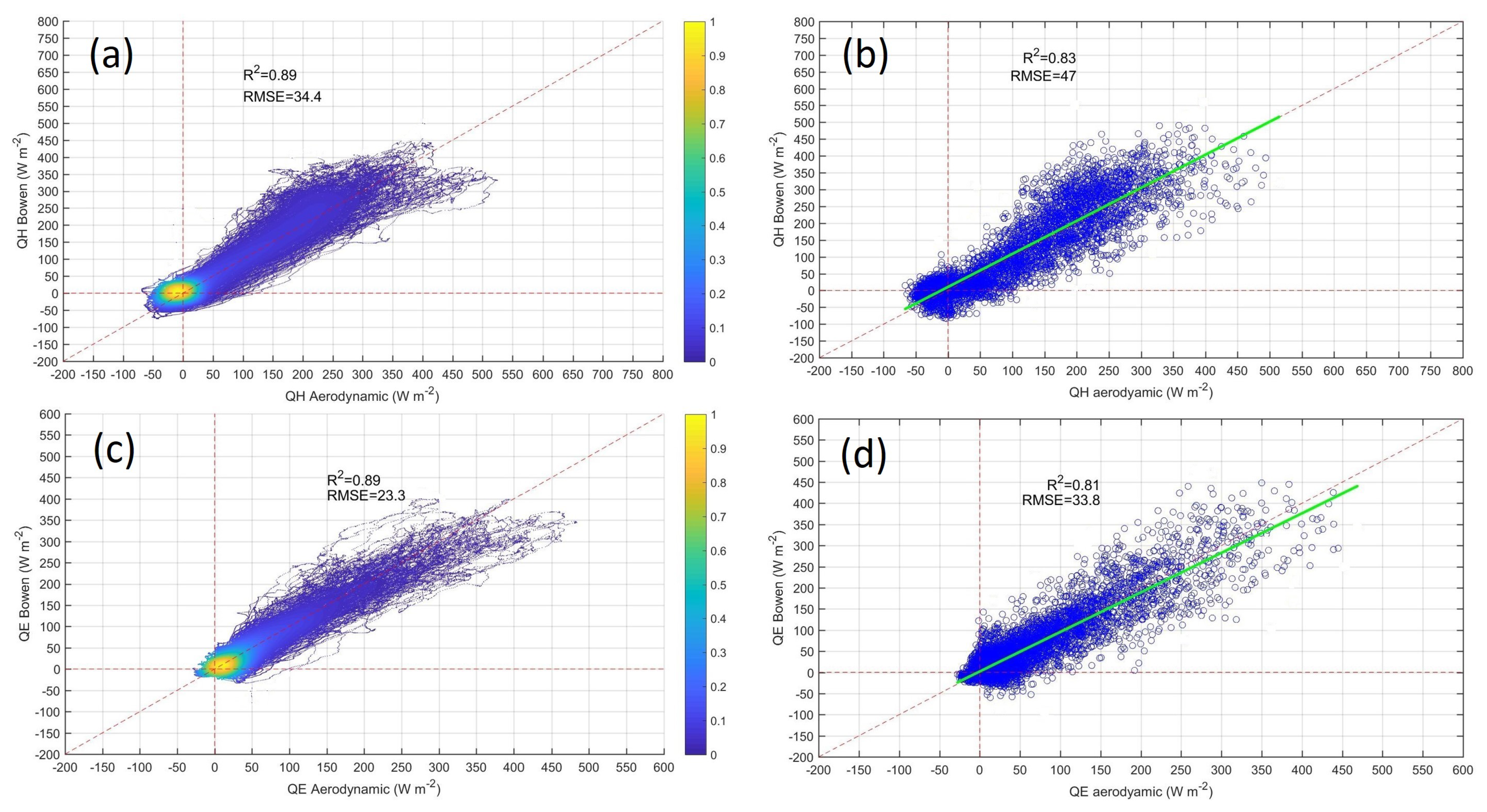
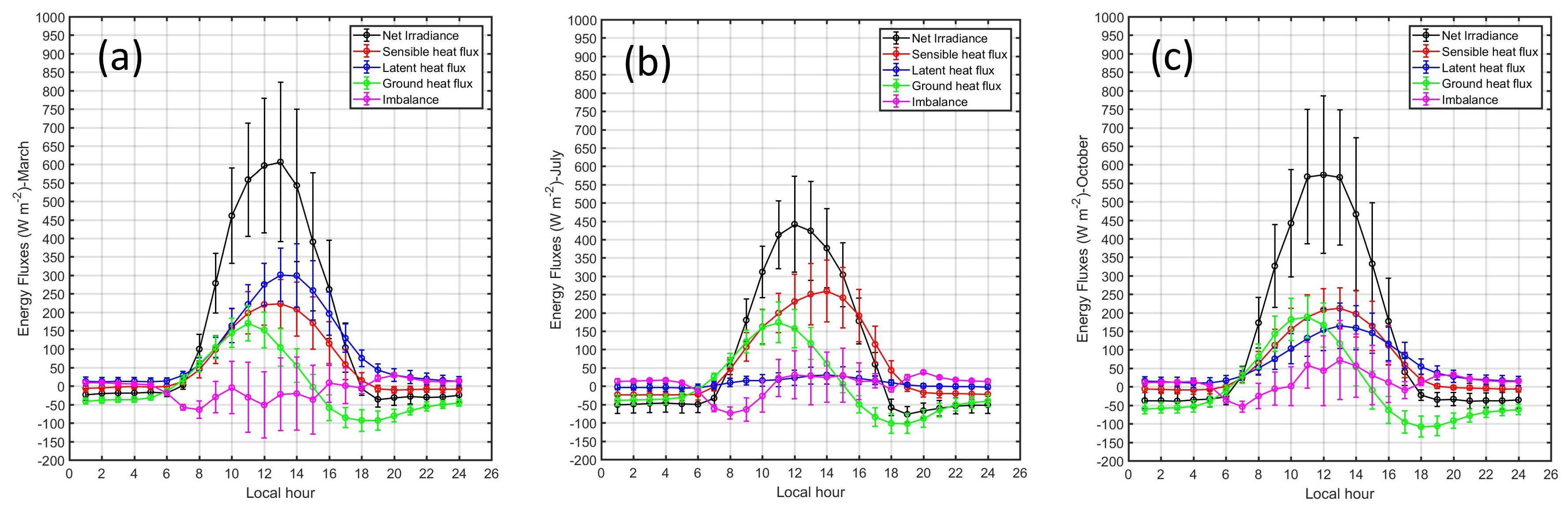
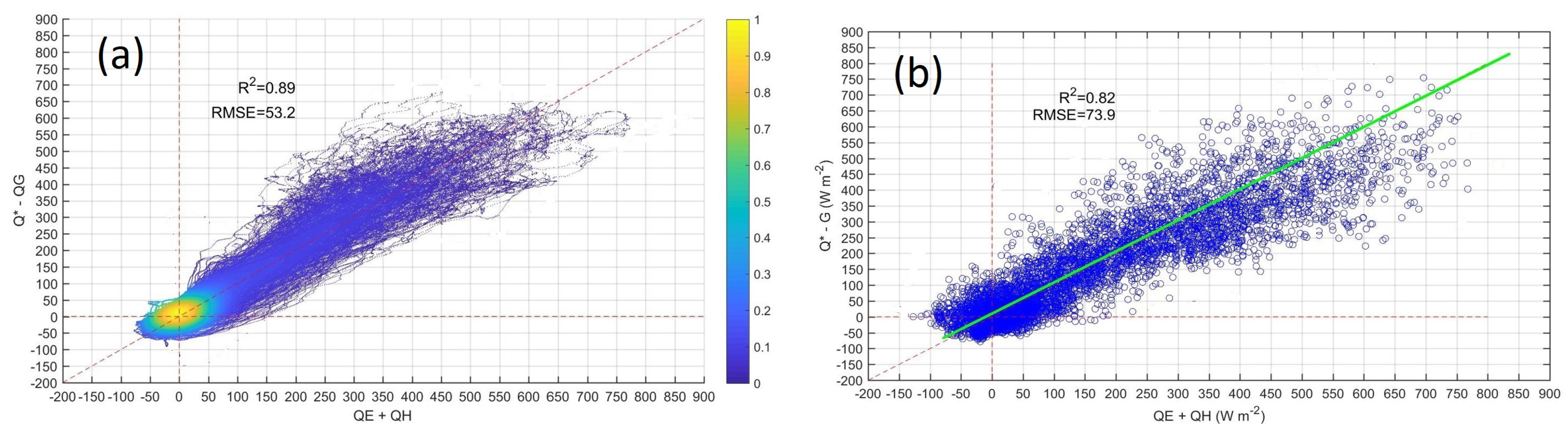
4.8. Energy-Balance Components and Imbalance

The sensible and latent heat fluxes estimated by the bulk aerodynamic method and by the Bowen-ratio energy-balance method (Section 3.3) were compared for the entire period of measurements (May 2018–April 2019). For the sensible heat flux ( Q H ) the comparison between both methods for the total data with 1 min resolution (444,960 points) (Figure 16a) and for the hourly mean values (7415 points) (Figure 16b) showed a good agreement.
For the total data, the coefficient of determination (R 2 ) is 0.89 and the RMSE is 34.4 W m 2 . For the hourly mean values, the overall values of R 2 is 0.83 and the RMSE is 47.0 W m 2 . These RMSE values are slightly higher than the instrumental accuracy of the Bowen-ratio energy- balance method [56]. The slope of the regression line is 0.98 and the intercept is 10.46 W m 2 . The Figures showed that the major departure of the regression line from the 1:1 line was observed for Q H values above 300 W m 2 . These values of Q H correspond to periods between 10 and 16 LT (Figure 14c).
For the latent heat flux ( Q E ), the results also indicated a good agreement (less than the case of Q H ) for the total data with 1 min resolution (444,960 data) (Figure 16c) and for the hourly mean values (7415 data) (Figure 16d). For total data, the coefficient of determination (R 2 ) is 0.89 and the RMSE is 23.3 W m 2 . For hourly mean values, the overall values of R 2 is 0.81 and the RMSE was 33.8 W m 2 . The slope of the regression line is 0.94 and the intercept was 2.12 W m 2 . The Figures showed that the major departure of the regression line from the 1:1 line was observed for sensible heat values above 250 W m 2 . These values of Q H correspond to periods between 10 and 16 LT (Figure 15c).
The daily cycle of the mean monthly values of the energy-balance components for March, July and October are shown in Figure 17a–c, respectively. At noon, the maximum mean monthly Q was found in November (660 W m 2 ) and the minimum in July 450 W m 2 . During night hours, the mean monthly Q reach values between −60 and −50 W m 2 for all months. In fall–winter months (May-September), the values of Q H exceed Q E with values between 200 and 300 W m 2 for Q H and between 25 and 100 W m 2 for Q E around noon.
In contrast, for summer months (February–April) the values of Q E exceeded Q H with values between 250 and 300 W m 2 for Q E and between 180 and 220 W m 2 for Q H around noon. In spring months (October–January) both turbulent fluxes ( Q H and Q E ) had similar values close to 250 W m 2 . The daily cycle of Q G showed a wave-like form with maximum between 130 W m 2 (April) and 240 W m 2 (September) around 11 LT and minimum between −50 W m 2 (April) and −150 W m 2 (September) around 18 LT. Moreover, during early morning and night hours, the loss of Q was most effectively replenished by conduction upwards from the soil ( Q G ) being the convective contribution from Q H and Q E least effective (around 20 W m 2 ). For all months Q G became close to zero around 15 LT.
The diurnal cycle of the mean monthly imbalance term (Equation (14)) during March, July and October also are shown in Figure 17a–c, respectively. For all months, after sunrise the imbalance became negative with minimums between −50 W m 2 and −80 W m 2 around 07 and 08 LT, next the imbalance increased up to values between −50 W m 2 and 0 W m 2 in March. However, in July, the imbalance becomes close to 0 W m 2 from 11 LT and remained with this value along the night. Finally, in October, the imbalance increased after 07 LT up to values up to values close to +50 W m 2 around 13 LT.
Later, in afternoon hours the imbalance continuously decreased up to values close to zero at night hours. Scatter plots for overall comparison between available energy ( Q − G) and the sum of latent heat and sensible heat ( Q E + Q H ) are shown in Figure 18a for all data with 1 min resolution (444,960 data) and Figure 18b for the hourly mean values (7415 data). For all data, the coefficients of determination (R 2 ) is 0.89 and the RMSE is 53.2 W m 2 . For the hourly mean values, the overall values of R 2 is 0.82 and the RMSE is 73.9 W m 2 . The slope of the regression line is 0.98 and the intercept is 10.24 W m 2 . The major departure of the regression line from the 1:1 line was observed for Q E + Q H values above 250 W m 2 . These values of Q E + Q H correspond to periods between 10 and 16 LT (Figure 17). The discussions of all results are presented in Section 5.

5. Discussions

5.1. Air Temperature

According to the results presented in Section 4.1, during winter months, at night and early morning hours, the surface boundary layer presented stable conditions with positive lapse rates around +0.25 C m 1 and Richardson numbers close to 0.1, which were generated when the surface cooled down to a temperature below that of the air above mainly due to the strong negative net LW irradiance (between −50 and −60 W m 2 ) caused by the low water vapor content, low precipitation, and low cloud cover, producing a ground-based radiation inversion. During these hours, the sensible heat flux ( Q H ) was negative, coming more intense in June and July (close to −25 W m 2 ). This divergence extended the cooling to affect a depth of around 30 m just before sunrise. The minimum mean monthly temperature at 2 m was found in July at 07 LT (1.8 C). These results agree with previous studies that found the most frequent frost events (below 0 C at 2 m) in the Huancayo observatory during June and July [19].
On the contrary, during summer months at early morning hours, the surface boundary layer presented slightly unstable conditions with a negative Richardson numbers between −0.2 and −0.5 due to an increase in the net SW irradiance (maximum around 50 W m 2 ) and the net LW irradiance (around −35 W m 2 ) that are caused by an increase in the water vapor content and precipitation and cloud cover. At these hours, Q H neared zero (around −5 W m 2 ), which leads to a decrease in the temperature differences between the surface and the higher atmosphere. The maximum mean monthly temperature at early morning hours was calculated in March at 07 LT (8.71 C). For transition seasons (fall-spring), moderate unstable conditions of the atmospheres with a lapse rate below 0.18 C m 1 were observed. After sunrise, the surface net irradiance ( Q ) became positive (Figure 17) and the air temperature reached its maximums between 18 C and 20 C around 16 LT for all months. Continued Q H convergence in the lowest atmosphere generates a deep unstable surface boundary layer with the maximum close to −0.25 C m 1 and Ri between −1.5 and −1.9, around 10 LT for all months. This condition generates an upward Q H that converges into the lowest air layer with the maximum values between 250 W m 2 (July) and 300 W m 2 (March) at 14 LT.

5.2. Air Moisture

The exchange of moisture between the surface and the boundary layer determines the humidity quantified as water mixing ratio. According to the results in Section 4.2, during winter months (June to August), at night and early morning hours, the water vapor vertical profiles become inverted near the surface below 6 m so that the vapor is transferred downwards as dewfall. This process depletes the moisture in the lowest layers and leads to a decrease in humidity. The water mixing ratio presented low values around 5 g kg 1 and Q E slightly negative values close to zero, indicating the formation of dewfall favored by the observed low wind speeds close to 0.5 m s 1 at 2 m. On the contrary, in summer months, the water vapor vertical profiles showed negative slopes at night and early morning hours, as a consequence of the transfer of moisture from the surface to the lower atmosphere caused by high precipitation rates during these months (Figure 13d). The water mixing ratio presented high values between 8.5 g kg 1 and 9.5 g kg 1 ; Q E also shows important positive values close to 20 W m 2 , which indicate a flux of water directed upward from the surface to the lower atmosphere.
In winter months, at day hours, the vapor vertical profiles remained almost constant with a slight increment from 12 to 30 m, probably due to the moisture from the south-easterly winds of the mountain valley circulation. After sunrise, the water vapor mixing ratio increases because of the addition of moisture due to the evapotranspiration of surface water into a moderately unstable atmosphere and reaches its maximum values between 5.5 and 6.5 g kg 1 at around 10 LT. By early afternoon, between 12 and 15 LT, the moisture content drops slightly in the surface boundary layer, probably due to dilution in mixture with dry air masses that descends from above as a result of the convective activity penetrating the top of the boundary layer. The continentality and altitude of the Huancayo observatory intensify these phenomena because regional air masses are dry and surface heating is strong, especially in fall–winter months, due to the absence of clouds. In the late afternoon, the surface boundary layer becomes stable because the surface cooling is strong and, as a consequence, has the ability to transport vapor to higher layers at a rate lesser than at which it continues to be added from the surface. As a result, moisture convergences into the lowest layers and a second humidity maximum is observed at around 20 LT; humidity declines into the night period.
In contrast, in summer months, at day hours, the water vapor vertical profiles show higher negative slopes than during the night with values close to −0.16 g kg 1 m 1 , because of the upward vapor being transported by eddy diffusion. The water vapor mixing ratio presents a similar behavior than that in winter months but with higher values between 9 and 10 g kg 1 in the day. Coinciding with the minimum temperatures, the diurnal cycle of RH reaches its maximum between 06 and 07 LT for all months with the minimums in July (∼75%) due to a low amount of moisture with values close to 4.5 g kg 1 and the maximum in March (∼90%) due to a high amount of moisture with values around 9.5 g kg 1 at 2 m. The vertical profiles of RH present strong negative lapse rates at night hours and slightly positive lapse rates at day hours for all months.

5.3. Wind Speed and Momentum Flux

The orientation of the Mantaro Valley from north-west to south-east favors the formation of local winds as a result of thermal differences (mountain–valley circulation), mostly under cloudless skies and weak synoptic conditions presented during fall–winter season in the Huancayo observatory. According to the results presented in Section 4.3, the wind field in the surface boundary layer was largely controlled by the underlying rigid surface that imposed frictional drag on the wind flow. As the surface approaches, the drag retards its motion close to the ground, which gives rise to a sharp decrease in the mean horizontal wind speed. This decrease with height was found to be greater for strong winds, around 17 and 18 LT, for all months. In winter months, the minimum wind speeds were observed around sunrise (06 LT) with values close to 0.5 m s 1 at 2 m. These values of wind speed favored the formation of dewfall during the hour mentioned above. The maximum wind speeds were observed at around 18 LT with values between 5.5 and 6 m s 1 in August. In summer months, the amplitude of the wind speed in the day were seen to decrease with the minimums close to 0.2 m s 1 at around 06 LT and maximums close to 2.0 m s 1 at around 15 LT. The flux of the momentum, which is a measure of the force exerted by the wind flow, on the surface reached its maximum of about 0.2 N m 2 at the moment of the highest vertical wind shear between 16 and 17 LT and minimum of around 0.036 N m 2 at 07 LT for all months.
By using the wind profiles in neutral conditions, the mean value of the roughness length ( z = 0.20) and the mean value of the friction velocity ( u = 0.29 m s 1 ) were estimated. These values correspond to the aerodynamic properties of crops at 0.5 m height. In general, neutral conditions were found under cloudy skies and strong winds because clouds reduced the radiative heating and cooling of the surface and strong winds promoted mixing and did not permit strong temperature stratification to develop; the lowest layers dominated forced convection due to eddies generated by friction with the surface. For the Mantaro Valley, these conditions are predominant between 16 and 19 LT for all months.

5.4. Soil and Surface Temperature and Moisture

According to the results presented in Section 4.4, heat transfer and thermal properties of soils are governed mainly by the volumetric heat capacity related to the ability of a substance to store heat and express the temperature change produced due to gaining or losing heat. The volumetric heat capacity is affected by different soil properties, especially soil moisture. In winter months, the near-soil temperature variation (2 cm deep) was found to be wave-like with the maximum around 38 C at 14 LT and the minimum close to 5 C at 07 LT. The wave was seen to penetrate downward to lower depths (5, 10 and 30 cm); however the amplitude decreased and the time periods of maximum and minimum temperature shifted to the right in time. At a depth of 50 cm the soil temperature was almost constant in the day with values around 16 C. The soil moisture behavior was similar to that of the soil temperatures for all depths with lower values near the surface (5% to 10%) and higher values at greater depths (20–24%). In contrast, in summer months, the amplitude of the near-soil temperature (2 cm depth) was found to be lower with the maximum around 30 C at 14 LT and the minimum around 12 C at 06 LT. At a depth of 50 cm, the soil temperature was almost constant along the day with values around 16 C. The soil moisture also presented lower amplitudes with closer values between 21% and 24% at a depth of 2 cm and around 26% for the other depths.
According to the results presented in Section 3.4, the LST estimated using the LW irradiance components was found to be associated to uncertainties in the range of 2–3 C [16] mainly because of the sensitivity of the long-wave radiation sensor and the uncertainty of the emissivity. In winter months, at night hours, the T2-LST had positive values between 0 and 1 C, which are small compared to the uncertainty of LST, indicating the presence of slightly stable stratification of the surface boundary layer as average condition for the Mantaro Valley. In contrast, in summer months, T2-LST had small negative values of around −1.4 C, indicating the presence of neutral or slightly unstable conditions in the lower atmosphere during the night. On the contrary, at day hours, T2-LST was negative with between −1.5 C after sunrise and −12 C at noon for all months, indicating the presence of highly unstable conditions of the surface boundary layer.
On the other hand, the surface albedo that depends on the state of the soil and vegetation presents a well-defined seasonal cycle estimated over the period from 10 to 17 LT. The lower values of the surface albedo were observed in rainy summer months (around 0.15) while the higher in dry winter months (around 0.21). Intermediate values (close to 0.18) were observed in transient seasons (fall-spring). This seasonal cycle of the surface albedo was found to be associated with the content of moisture of the natural vegetation canopy that depends entirely of the seasonal cycle of the rainfall that falls on the surface (Figure 13d). The Bowen ratio ( β ) also presents a well-defined seasonal cycle with the highest values in the dry winter months between 6 and 14 and lowest values in rainy summer months with values between 2 and 5. Again, intermediate values (between 2 and 10) were observed in transient seasons (fall-spring). These values of β are consistent with the seasonal variation of Q E and Q H and show the prevailing conditions above the Huancayo observatory were semi-arid in spring–summer months and arid in fall–winter months. It should be noted that these values of β can be sub or overestimated due to the errors associated with the profiles methods to estimate turbulent energy fluxes and because the method does not into account the imbalance components of the energy budget.

5.5. Energy-Balance Components and Imbalance

According to the results presented in Section 4.8, the most important difference between the aerodynamic method and the Bowen-ratio energy-balance method to estimate the turbulent energy fluxes is that the latter presumes a perfect balance between the traditional energy-balance elements while the former allows the existence of imbalance terms because it does not assume a perfect balance. However, it should be noted that both are approximate methods, and a better estimation of turbulent energy fluxes ( Q H and Q E ) is by using an eddy covariance equipment, as verified by several studies [10,15,16,18,57]. Despite this, as the first approximation, the imbalance term in Equation (14) was estimated by using the turbulent energy-balance fluxes using the aerodynamic method.
In this context, the comparison between the Q H and Q E made by the two methods shows a good agreement with the coefficient of determination (R 2 ) above 0.8 and the RMSE between 10 W m 2 and 30 W m 2 for both Q H and Q E . Moreover, the slope of the regression line between the two methods is greater than 0.94, and the intercept has values between 2 W m 2 and 10 W m 2 . The comparison between the available energy ( Q Q G ) and the turbulent energy fluxes estimated by the aerodynamic method ( Q H + Q E ) also shows a good level of agreement similar to the made between the individual terms (R 2 > 0.8 and slope of the regression line above 0.95).
The components of the energy budget showed a seasonal and daily variation. The exact partitioning of Q between Q H , Q E , and Q G was governed by the relative abilities of the soil and the atmosphere to transport heat and the physical properties of the surface. At noon, the mean monthly value of Q reached its maximum in November (660 W m 2 ) and its minimum in July (450 W m 2 ). In fall–winter months, the mean monthly value of Q H (maximum close to 300 W m 2 at noon) exceeds the mean monthly value of Q E (maximum close to 100 W m 2 at noon) due to the poor soil moisture available during this period. On the contrary, in spring–summer months, the opposite occurred; the mean monthly value of Q E (maximum close to 300 W m 2 at noon) exceeded the mean monthly value of Q H (maximum close to 220 W m 2 at noon) because of the high precipitation that occurred during this period (Figure 13d), which enhanced the soil moisture availability in the Mantaro valley. Moreover, the nocturnal Q loss is most effectively replenished by Q G than by the turbulent fluxes. This effect is more evident in winter months when Q E is almost insignificant at night and the atmosphere is stratified due to the low surface temperatures and low soil moisture.
The imbalance term (Equation (14)) also showed a seasonal and daily variation. For all months, after sunrise the imbalance became negative with values between −50 W m 2 and −80 W m 2 . Next, the imbalance increased up to reach positive values with the minimum close to zero (July) and the maximum close to +50 W m 2 (October). Apart from the instrumental errors and the errors associated with the methods to estimate turbulent energy fluxes, these values for the imbalance can be seen due to the long-lasting terrain heterogeneities on the hectometer (100 m) scale [15,16]. The surface on which the sensors measured the meteorological variables is a natural vegetation canopy that it is not irrigated at any time of the year. In contrast, surrounding this natural canopy, there are several cultivated fields and small woods that are frequently irrigated (Figure 1c). This contrast can explain a significant part of the imbalance, especially after sunrise and at noon, as the temperature gradients may generate motions that last longer than the averaging time of the turbulent fluxes [15,16]. Moreover, the mountain–valley circulation can also contribute to the enhance of the advective process of energy [58]. However, more conclusive evidence is needed to verify these hypotheses by performing experiments specifically designed to estimate the sign of the advection term.

6. Conclusions

The present study conducted a detailed analysis of the diurnal and monthly cycles of the surface boundary layer and, surface energy balance in a sparse natural vegetation canopy on the Huancayo observatory (12.04 S, 75.32 W, 3313 m asl) located in the central Andes of Perú (Mantaro valley) during an entire year (May 2018–April 2019). According to the results and discussions presented above, the following conclusion was made:
The period of minimum mean temperature and the high stable conditions of the the surface boundary layer occurred at early morning hours (between 06 and 07 LT) of fall-winter months (May–July). This period coincided with that of the highest negative net irradiance (SW + LW), highest positive Richardson number, lower vapor content and absence of precipitation in previous days. There is also a great divergence in sensible heat flux ( Q H ), which extends the cooling effect up to a depth of above 30 m before sunrise. On the contrary, the maximum mean temperature has less pronounced seasonal variability, with maximum intensities in spring months (September -November) at around 16 LT and highly unstable conditions at 11 LT. During these hours, high convergence of sensible heat flux ( Q H ) with maximums at 14 LT were observed for all months.
The transfer of water as dewfall at night and early morning hours of winter months was evident by the inversion of the water vapor vertical profiles below 6 m, by the slightly negative values of latent heat flux ( Q E ), and the low wind speeds that favored the formation of dewfall. In contrast, in summer months, at night and early morning hours, the water vapor vertical profiles showed negative slopes due to the transfer of moisture from the surface to the lower atmosphere, which is caused by high precipitation rates, high values of water mixing ratio, and positive values of Q E that indicate a flux of water directed upward from the surface to the lower atmosphere. At day hours, the water vapor vertical profiles were almost constant with the highest in winter months due to lower availability of moisture. However, in summer months, the profiles presented strong negative slopes due to a high amount of moisture in the surface and high values of Q E .
A well defined mountain-valley circulation was seen to change from east and south-east at day hours to west and south-west at night hours. This thermal circulation was more defined in fall-winter months under cloudless skies and weak synoptic conditions. The maximum wind speeds were observed between 17 and 18 LT while the minimum at early morning hours for all months. The mean value of the roughness length ( z ) was estimated as 0.20 and the mean value of the friction velocity ( u ) as 0.29 m s 1 using wind profiles in neutral conditions, which were found to be predominantly between 16 and 19 LT under cloudy skies and strong winds for all months.
The observed variability of the soil temperature showed a well-known wave propagation with higher amplitudes close to the surface and almost constant values at a depth of 50 cm with the maximum at noon and the minimum at early morning hours. The amplitudes of temperature were found to be higher in dry months than in wet months. This behavior was consistent with the diurnal and seasonal cycle of the soil moisture content, which is low in dry months and high in wet months. As a consequence, the highest specific heat capacity of water maintains the soil temperatures with lower amplitudes during the day. The LST was estimated using the LW irradiance emitted by the surface and incident from the atmosphere. The difference between air temperature at a depth of 2 m and the LST (T2-LST) only presented positive values at night and early morning hours of winter months, indicating the presence of stable stratification of the surface boundary layer as the average condition. For diurnal hours, the difference (T2-LST) exhibited negative values, indicating the presence of unstable conditions at the surface boundary layer. The surface albedo and the Bowen ratio ( β ) showed a well defined seasonal cycle according to the characteristics of the soil and vegetation canopy. The former was higher (lower) in winter (summer) months when the vegetation and the soil were dry (moist) with values ranging from 0.15 to 0.21. In contrast, the Bowen ratio was higher (lower) in summer (winter) months when the moisture availability caused by precipitation was high (low) with values ranging from 2 to 14. The seasonal variation of β was consistent with that Q E and Q H . According the variation of β , the prevailing conditions for the Huancayo observatory were semi-arid during wet months and arid during dry months.
Besides the differences between both profiles methods to estimate the turbulent energy fluxes ( Q E and Q H ) based on the assumption (or not) of perfect energy balance between the traditional components, the comparison between the two methods (aerodynamic and Bowen ratio energy balance) shows a good level of agreement with R 2 above 0.8 and RMSE between 10 and 30 W m 2 . The partitioning of Q was governed by the relative abilities of the soil and the atmosphere to transport heat and by the physical properties of the surface canopy. In winter months, a strong predominance of Q H in relation with Q E was observed, and in summer months the opposite was seen, mainly due to the seasonal cycle of precipitation and moisture. Moreover, the imbalance term showed a seasonal and daily variation probably associated with the surface long-lasting terrain heterogeneities at the hectometer (100 m) scale around the Huancayo observatory, which led to the advective process of energy enhancement by the mountain valley circulation. However, more conclusive evidence is required to verify these hypothesis by performing experiments specifically designed to estimate the sign of the advection term.

Author Contributions

For the present work, the contributions were distributed as follows: conceptualization, J.L.F.-R. and J.C.; methodology, J.L.F.-R. and M.P.-L.; software, J.L.F.-R. and J.C.; validation, J.L.F.-R., M.P.-L. and S.C.; formal analysis, J.L.F.-R. and S.K.; investigation, J.L.F.-R., J.C. and S.C.; resources, L.S.-S., Y.S.-V. and A.S.M.-A.; data curation, M.P.-L. and S.C.; writing—original draft preparation, J.L.F.-R.; writing—review and editing, J.L.F.-R.; visualization, J.L.F.-R. and A.S.M.-A.; supervision, Y.S.-V. and J.C.; project administration, Y.S.-V.; funding acquisition, Y.S.-V.

Funding

This research received no external funding.

Acknowledgments

We wish to thank to the “Consejo Nacional de Ciencia y Tecnologia” (CONCYTEC) (Nro 010-2017-FONDECYT) and to the "INNOVATE PERU" (Nro 400-PNIC-2015) for the financial support during the research period. This work was done using computational resources, HPC-Linux -Cluster, from Laboratorio de Dinámica de Fluidos Geofísicos Computacionales at Instituto Geofísico del Perú (grants 101-2014-FONDECYT, SPIRALES2012 IRD-IGP, Manglares IGP-IDRC, PP068 program).Thanks to the Ministry of External Affairs of Peru and WMO/GCOS programme for facilitating the implementation of BSRN station. J.C. was supported by the project RTI2018-098693-B-C31 (MICINN and AEI) of the Spanish Government, with funding from the European Regional Development Fund (FEDER-EU).

Conflicts of Interest

The authors declare no conflict of interest.

Abbreviations

The following abbreviations are used in this manuscript:
PBLPlanetary boundary layer
SBLSurface boundary layer
ImbImbalance term
LWLong-Wave irradiance
SWShort-wave irradiance
WMOWorld Meteorological Organization

References

  1. Stull, R.B. An Introduction to Boundary Layer Meteorology; Kluwer Academic Publishers: Dordrecht, The Netherlands, 2003. [Google Scholar]
  2. Arya, S. Introduction to Micrometeorology, 2nd ed.; Academic Press: Cambridge, MA, USA, 1998. [Google Scholar]
  3. Garratt, J. Review: The atmospheric boundary layer. Earth Sci. Rev. 1994, 37, 89–134. [Google Scholar] [CrossRef]
  4. Rigby, J.; Jin, Y.; Albertson, J.; Porporato, A. Approximate analytical solution to diurnal Atmospheric Boundary Layer growth under well-watered conditions. Bound.-Layer Meteorol. 2015, 156. [Google Scholar] [CrossRef]
  5. Busch, N. The surface boundary layer. Bound.-Layer Meteorol. 1973, 4, 213–240. [Google Scholar] [CrossRef]
  6. Monteith, J.; Unsworth, M. Principles of Environmental Physics, 1st ed.; Edward Arnold: London, UK, 1990; p. 291. [Google Scholar]
  7. Oke, T. Boundary Layer Climates, 2nd ed.; Taylor and Francis Group: London, UK, 1987. [Google Scholar]
  8. Prueger, J.; Kustas, W. Aerodynamic Methods for Estimation Turbulent Fluxes, 1st ed.; USDA-ARS/UNL Faculty: Lincoln, Nebraska, 2005; p. 1394. [Google Scholar]
  9. Piere, P.; Fuch, M. Comparison of Bowen ratio and aerodynamic estimates of evapotranspiration. Agric. For. Meteorol. 1990, 49, 243–256. [Google Scholar] [CrossRef]
  10. Kalthoff, N.; Fiebig-Wittmaack, M.; Meißner, C.; Kohler, M.; Uriarte, M.; Bischoff-Gauß, I.; Gonzales, E. The energy balance, evapo-transpiration and nocturnal dew deposition of an arid valley in the Andes. J. Arid Environ. 2006, 65, 420–443. [Google Scholar] [CrossRef]
  11. Geiger, R.; Aron, R.; Todhunter, P. The Climate Near the Ground, 1st ed.; Rowman & Littlefield Publishing Inc.: Lanham, MD, USA, 2003. [Google Scholar]
  12. LeMone, M.; Ikeda, K.; Grossman, R.; Rotach, M. Horizontal variability of 2 m temperature at night during CASES-97. J. Atmos. Sci. 2003, 60, 2431–2449. [Google Scholar] [CrossRef]
  13. Eder, F.; Serafimovich, A.; Foken, T. Coherent structures at a forest edge: Properties, coupling and impact of secondary circulations. Bound.-Layer Meteorol. 2013, 148, 285–308. [Google Scholar] [CrossRef]
  14. Marth, L. Computing turbulent fluxes near the surface: Needed improvements. Agric. For. Meteorol. 2010, 150, 501–509. [Google Scholar]
  15. Cuxart, J.; Wrenger, B.; Martínez-Villagrasa, D.; Reuder, J.; Jonassen, M.O.; Jiménez, M.A.; Lothon, M.; Lohou, F.; Hartogensis, O.; Dünnermann, J.; et al. Estimation of the advection effects induced by surface heterogeneities in the surface energy budget. Atmos. Chem. Phys. 2016, 16, 9489–9504. [Google Scholar] [CrossRef] [Green Version]
  16. Simó, G.; Cuxart, J.; Jiménez, M.; Martínez-Villagrasa, D.; Picos, R.; López-Grifol, A.; Martí, B. Observed atmospheric and surface variability on heterogeneous terrain at the hectometer scale and related advective tranports. J. Geophys. Res. Atmos. 2019, 124. [Google Scholar] [CrossRef]
  17. Foken, T. The energy balance closure problem: An overview. Ecol. Appl. 2008, 18, 1351–1367. [Google Scholar] [CrossRef] [PubMed]
  18. Cuxart, J.; Conangla, L.; Jiménez, M. Evaluation of the surface energy budget equation with experimental data and the ECMWF model in the Ebro Valley. J. Geophys. Res. Atmos. 2015, 120, 1008–1022. [Google Scholar] [CrossRef] [Green Version]
  19. Saavedra, M.; Takahashi, K. Physical controls on frost events in the central Andes of Peru using in situ observations and energy flux models. Agric. For. Meteorol. 2017, 239, 58–70. [Google Scholar] [CrossRef]
  20. Sulca, J.; Vuille, M.; Silva, Y.; Takahashi, K. Teleconnections between the Peruvian Central Andes and Northeast Brazil during extreme rainfall events in Austral summer. J. Hydrometeorol. 2015, 17, 499–515. [Google Scholar] [CrossRef]
  21. Moya-Álvarez, A.; Gálvez, J.; Holguín, A.; Estevan, R.; Kumar, S.; Villalobos, E.; Martínez-Castro, D.; Silva, Y. Extreme Rainfall Forecast with the WRF-ARW Model in the Central Andes of Peru. Atmosphere 2018, 9, 362. [Google Scholar] [CrossRef] [Green Version]
  22. Kumar, S.; Silva-Vidal, Y.; Moya-Álvarez, A.; Martínez-Castro, D. Effect of the surface wind flow and topography on precipitating cloud systems over the Andes and associated Amazon basin: GPM observations. Atmos. Res. 2019, 1. [Google Scholar] [CrossRef]
  23. Flores-Rojas, J.; Moya-Alvarez, A.; Kumar, S.; Martínez-Castro, D.; Villalobos-Puma, E.; Silva-Vidal, Y. Analysis of Possible Triggering Mechanisms of Severe Thunderstorms in the Tropical Central Andes of Peru, Mantaro Valley. Atmosphere 2019, 10, 301–331. [Google Scholar]
  24. Martínez-Castro, D.; Kumar, S.; Flores-Rojas, J.; Moya-Álvarez, A.; Valdivia-Prado, J.; Villalobos-Puma, E.; Castillo-Velarde, C.; Silva-Vidal, Y. The Impact of Microphysics Parameterization in the Simulation of Two Convective Rainfall Events over the Central Andes of Peru Using WRF-ARW. Atmosphere 2019, 10, 442. [Google Scholar] [CrossRef] [Green Version]
  25. Moya-Álvarez, A.; Estevan, R.; Kumar, S.; Flores-Rojas, J.; Ticse, J.; Martínez-Castro, D.; Silva-Vidal, Y. Influence of PBL parameterization schemes in WRF-ARW model on short-range precipitation’s forecasts in the complex orography of Peruvian Central Andes. Atmos. Res. 2019, 1. [Google Scholar] [CrossRef]
  26. Yin, J.; Albertson, J.; Rigby, J.; Porporato, A. Land and atmospheric controls on initiation and intensity of moist convection: CAPE dynamics and LCL crossings. Water Resour. Res. 2015, 51, 8476–8493. [Google Scholar] [CrossRef]
  27. Pascale, S.; Lucarini, V.; Feng, X.; Porporato, A.; Hasson, S. Analysis of rainfall seasonality from observations and climate models. Clim. Dyn. 2015, 44, 3281–3301. [Google Scholar] [CrossRef] [Green Version]
  28. Feng, X.; Porporato, A.; Rodriguez-Iturbe, I. Changes in rainfall seasonality in the tropics. Nat. Clim. Chang. 2013, 3, 811–815. [Google Scholar] [CrossRef]
  29. Silva, Y.; Trasmonte, G.; Giráldez, L. Variabilidad de las Lluvias en el Valle del Mantaro Memoria del Subproyecto: Pronóstico Estacional de Lluvias Y Temperatura en la Cuenca del río Mantaro Para su Aplicación en la Agricultura; Fondo Editorial CONAM-Instituto Geofísico del Perú: Lima, Peru, 2010. [Google Scholar]
  30. IGP. Atlas Climático de Precipitación y Temperatura del Aire en la Cuenca del río Mantaro. Volumen I; Fondo Editorial CONAM-Instituto Geofísico del Perú: Lima, Peru, 2005. [Google Scholar]
  31. Trasmonte, G.; Silva, Y.; Segura, B.; Latínez, K. Variabilidad de las Temperaturas máximas y mínimas en el Valle del Mantaro. Memoria del Subproyecto “Pronóstico Estacional de Lluvias y Temperatura en la Cuenca del río Mantaro Para su Aplicación en la Agricultura”; Fondo Editorial CONAM-InstitutoGeofísico del Perú: Lima, Peru, 2010. [Google Scholar]
  32. Jammalamadaka, S.; Sengupta, A. Topics in Circular Statistics. World Sci. Singap. 2001, 5, 1–20. [Google Scholar]
  33. Yin, J.; Porporato, A. Diurnal cloud cycle biases in climate models. Nat. Commun. 2017, 8, 2269. [Google Scholar] [CrossRef] [Green Version]
  34. Berens, P. CircStat: A MATLAB toolbox for Circular Statistics. J. Stat. Softw. 2009, 31, 1–20. [Google Scholar] [CrossRef] [Green Version]
  35. Bowen, I. The ratio of heat losses by conduction and by evaporation from any water surface. Phys. Rev. 1926, 27, 779–787. [Google Scholar] [CrossRef] [Green Version]
  36. Monin, A.; Obukhov, A. Basic laws of turbulent mixing in the ground layer of the atmosphere. Contrib. Geophys. Inst. Acad. Sci. USSR 1954, 151, e187. [Google Scholar]
  37. Foken, T.; Richter, S.; Muller, H. Zur Genauigkeit der Bowen-Ratio-Methode. Wetter und Leben 1997, 49, 57–77. [Google Scholar]
  38. Ohmura, A. Objective criteria for rejecting data for Bowen ratio flux calculations. J. Appl. Meteorol. 1982, 21, 595–598. [Google Scholar] [CrossRef] [Green Version]
  39. Malek, E.; McCurdy, G.; Giles, B. Evaporation from margin and moist playa of a closed desert valley. J. Hydrol. 1990, 120, 15–34. [Google Scholar] [CrossRef]
  40. Malek, E.; Bingham, G. Partinioning of radiation and energy balance components in an inhomogeneous desert valley. J. Arid. Environ. 1997, 37, 193–207. [Google Scholar] [CrossRef]
  41. Malek, E.; McCurdy, G.; Giles, B. Dew contribution to the annual water balances in semi-arid desert valleys. J. Arid. Environ. 1999, 42, 71–80. [Google Scholar] [CrossRef]
  42. Beringer, J.; Tapper, N. The influence of subtropical cold fronts on the surface energy balance of a semi-arid site. J. Arid. Environ. 2000, 44, 437–450. [Google Scholar] [CrossRef]
  43. Silva, B.; Strobl, S.; Beck, E.; Bendix, J. Canopy evapotranspiration, leaf transpiration and water use efficiency of an andean pasture in SE-Ecuador—A case study. Erdkunde 2016, 70, 5–18. [Google Scholar] [CrossRef]
  44. Foken, T.; Nappo, C. Micrometeorology, 1st ed.; Springer: Berlin/Heildelberg, Germany, 2008. [Google Scholar]
  45. Oncley, S.; Foken, T.; Vogt, R.E.A. The Energy Balance Experiment EBEX-2000. Part I: Overview and energy balance. Bound.-Layer Meteorol. 2007, 123, 1–28. [Google Scholar] [CrossRef]
  46. Foken, T.; Mauder, M.; Liebethal, C.; Wimmer, F.; Beyrich, F.; Leps, J.; Raasch, S.; DeBruin, H.A.R.; Meijninger, W.; Bang, J. Energy balance closure for the LITFASS-2003 experiment. Theor. Appl. Climatol. 2010, 101, 149–160. [Google Scholar] [CrossRef]
  47. Garratt, J. The Atmospheric Boundary Layer, 2nd ed.; Cambridge University Press: Cambridge, UK, 1992. [Google Scholar]
  48. Mauder, M.; Oncley, S.; Vogt, R.; Weidinger, T.; Ribeiro, L.; Bernhofer, C.; Foken, T.; Kohsiek, W.; De Bruin, H.; Liu, H. The energy balance experiment EBEX-2000. Part II: Intercomparison of eddy-covariance sensors and post-field data processing methods. Bound.-Layer Meteorol. 2007, 123, 29–54. [Google Scholar] [CrossRef]
  49. Leuning, E.; Van Gorsela, E.; Massman, W.; Isaac, P. Reflections on the surface energy imbalance problem. Agric. For. Meteorol. 2012, 156, 65–74. [Google Scholar] [CrossRef]
  50. Porteous, A. Dictionary of Environmental Science and Technology, 4th ed.; Chinchester: New York, NY, USA, 1994; p. 439. [Google Scholar]
  51. Platero Morejón, I.; Esteban Arredondo, R.; García Parrado, F. Climatology of surface albedo at Camaguey Actinometric Station. Opt. Pura Apl. 2015, 48, 259–269. [Google Scholar] [CrossRef]
  52. WMO. Guide to Climatological Practices, 2nd ed.; WMO: Geneva, Switzerland, 2011. [Google Scholar]
  53. Simó, G.; Martínez-Villagrasa, D.; Jiménez, M.; Caselles, V.; Cuxart, J. Impact of the Surface—Atmosphere Variables on the Relation Between Air and Land Surface Temperatures. Pure Appl. Geophys. 2018, 175, 3939–3953. [Google Scholar] [CrossRef]
  54. Snyder, W.; Wan, Z.; Zhang, Y.; Feng, Y. Classification based emissivity for land surface temperature measurement from space. J. Remote. Sens. 1998, 14, 2753–2774. [Google Scholar] [CrossRef]
  55. Garay, O.; Ochoa, A. Primera AproximacióN Para la Identificación de los Diferentes tipos de Suelo Agrícola en el Valle del río Mantaro, 1st ed.; Instituto Geofísico del Perú: Lima, Peru, 2010. [Google Scholar]
  56. Ortega-Farias, S.; Cuenca, R.; Ek, M. Daytime variation of sensible heat flux estimated by the bulk aerodynamic method over a grass canopy. Agric. For. Meteorol. 1996, 81, 131–143. [Google Scholar] [CrossRef]
  57. Kleier, C.; Rundel, P. Energy balance and temperature relations of Azorella compacta, a high elevation cushion plant of the central Andes. Plant Biol. 2009, 11, 351–358. [Google Scholar] [CrossRef] [PubMed]
  58. Khodayar, S.; Kalthoff, N.; Fiebig-Wittmaack, M.; Kohler, M. Evolution of the atmospheric boundary-layer structure of an arid Andes Valley. Meteorol. Atmos. Phys. 2008, 99, 181–198. [Google Scholar] [CrossRef]
Figure 1. (a) The domain of the Mantaro valley and the location of the weather station in the Huancayo observatory of the “Instituto Geofísico del Perú” (12.05 S, 75.32 W, 3313 m asl). (b) Topography around the Mantaro valley, with higher altitudes close to 5000 m asl. (c) Images of the USGS Earth Explorer (https://earthexplorer.usgs.gov/) that shows the surface canopy around the Huancayo observatory. The red square at left side indicates the area of the observatory highlighted at right side.
Atmosphere 10 00779 g001
Figure 2. (a) Gradient tower located in the Huancayo observatory with sensors installed at six height levels: 2, 6, 12, 18, 24, and 29 m. (b) Anemometer (03101) with three cups from Campbell Scientific to measure wind speed. (c) Wind wane (024A) from Campbell Scientific which measure wind direction. (d) Air temperature and relative humidity (RH) probe (HMP60) from Campbell Scientific. (e) Soil heat flux plate (HFP01) measures the rate of energy transferred through a surface.
Atmosphere 10 00779 g002
Figure 3. (a) Tower located in the Huancayo observatory with radiation sensors installed at 6 m high. (b) Pyranometer (CMP10) manufactured by Kipp & Zonen which is an instrument that monitors solar irradiance for the full solar spectrum range. (c) Pyrgeometer (CGR4) from Kipp & Zonen, which is an instrument for the highest quality scientific measurements of LW irradiance. (d) Pyrheliometer CHP1 from Kipp & Zonen designed to measure of direct SW irradiance.
Atmosphere 10 00779 g003
Figure 4. (a) Wind direction dataset shown as points on the unit circle and (b) the same dataset shown as angular histograms. Red lines indicate the direction and magnitude of the mean resultant vector. To generate plots we used the algorithms presented in Berens’s contribution [34].
Atmosphere 10 00779 g004
Figure 5. Diurnal cycle of mean monthly values and standard deviations of (a) air temperature ( C) at 2 and 29 m, (b) relative humidity (%) at 2 and 29 m, (c) water mixing ratio (g kg 1 ) at 2 and 29 m and (d) soil heat flux (W m 2 ) at 8 cm depth during July 2018.
Atmosphere 10 00779 g005
Figure 6. Diurnal cycle of mean monthly values and standard deviations of (a) air temperature ( C) at 2 and 29 m, (b) relative humidity (%) at 2 and 29 m, (c) water mixing ratio (g kg 1 ) at 2 and 29 m and (d) soil heat flux (W m 2 ) at 8 cm depth during March 2019.
Atmosphere 10 00779 g006
Figure 7. Diurnal cycle of mean monthly vertical profiles of (a) air temperature ( C), (b) relative humidity (%), (c) water mixing ratio (g kg 1 ), and (d) wind speed (m s 1 ) from 2 to 29 m during July 2018.
Atmosphere 10 00779 g007
Figure 8. Diurnal cycle of mean monthly vertical profiles of (a) air temperature ( C), (b) relative humidity (%), (c) water mixing ratio (g kg 1 ), and (d) wind speed (m s 1 ) from 2 to 29 m during March 2019.
Atmosphere 10 00779 g008
Figure 9. Diurnal cycle of mean monthly values and standard deviations of (a) wind speed (m s 1 ) at 2 and 29 m, (b) wind direction at 18 and 29 m (degrees) (c) soil temperatures ( C) and (d) soil moisture at 2, 5, 10, 30 and 50 cm depth during July 2018.
Atmosphere 10 00779 g009
Figure 10. Diurnal cycle of mean monthly values and standard deviations of (a) wind speed (m s 1 ) at 2 and 29 m, (b) wind direction at 18 and 29 m (degrees) (c) soil temperatures ( C) and (d) soil moisture at 2, 5, 10, 30 and 50 cm depth during March 2019.
Atmosphere 10 00779 g010
Figure 11. Wind speed profile for neutral stability conditions of the atmosphere for (a) June 2 at 1649 LT, u = 0.34, z = 0.24, (b) July 14 at 1827 LT, u = 0.40, z = 0.1, (c) August 28 at 1737 LT, u = 0.59, z = 0.080.
Atmosphere 10 00779 g011
Figure 12. Diurnal cycle of mean monthly and standard deviations of LW irradiance components (W m 2 ) during (a) July 2018 and (c) March 2019. Diurnal cycle of mean monthly surface temperatures ( C) during (b) July 2018 and (d) March 2019.
Atmosphere 10 00779 g012
Figure 13. Diurnal cycle of mean monthly values and standard deviations of SW irradiance components (W m 2 ) for (a) February 2018 and (b) October 2018. (c) Diurnal cycle of mean monthly values of albedo for July, October and March. The values were calculated for zenith angles less than 70 covering an interval of 6 h from 09 to 15 LT. (d) Mean monthly and maximum daily of accumulated precipitation (mm) during 2018 registered by in situ pluviometer.
Atmosphere 10 00779 g013
Figure 14. Diurnal cycle of mean monthly values and standard deviations of (a) SW irradiances (W m 2 ), (b) Bowen ratio, (c) turbulent heat fluxes (W m 2 ), (d) momentum flux (N m 2 ) and Richardson number during July 2018.
Atmosphere 10 00779 g014
Figure 15. Diurnal cycle of mean monthly values and standard deviations of (a) SW irradiances (W m 2 ), (b) Bowen ratio, (c) turbulent heat fluxes (W m 2 ), (d) momentum flux (N m 2 ) and Richardson number during March 2019.
Atmosphere 10 00779 g015
Figure 16. Scatter plots for overall comparison between sensible heat flux estimated by aerodynamic technique ( Q H Aerodynamic) and Bowen ratio energy-balance method ( Q H Bowen) for (a) total data (1 min) and (b) Hourly mean values between May 2018 to April 2019. In (a) the color scale indicates the density of points. In (b) the grid line indicates the line of the regression with equation: Y = 0.98 X + 10.46. The same than (a,b) but for the latent heat flux ( Q E ) for (c) total data (1 min) and (d) Hourly mean values. In (c) the color scale indicates the density of points. In (d) the green line indicates the line of the regression with equation: Y = 0.94 X + 2.12.
Atmosphere 10 00779 g016
Figure 17. Daily cycle of the mean monthly values and standard deviations of the energy-balance components: net irradiance ( Q ), sensible heat flux ( Q H ), latent heat flux ( Q E ), ground heat flux ( Q G ) and of the imbalance term (Imb) for (a) March 2019, (b) July 2018 and (c) October 2018.
Atmosphere 10 00779 g017
Figure 18. Scatter plot for overall comparison between available energy ( Q − G) and the sum of latent heat and sensible heat ( Q E + Q H ) for (a) total data (1 min) (R 2 = 0.86; RMSE = 52.5 W m 2 ) and (b) Hourly mean values (R 2 = 0.83; RMSE = 68.9 W m 2 ) between May to September (2018). In (a) the color scale indicates the density of points. In (b) the green line indicates the line of the regression with equation: Y = 0.98 X + 11.13.
Atmosphere 10 00779 g018
Table 1. Main characteristics of the meteorological instrumentation installed in the Huancayo observatory.
Temperature
( C)
Relative
Humidity (%)
Wind
Speed (m s 1 )
Wind Direction
(degrees)
Soil Heat
Flux (W m 2 )
Soil
Temperature ( C)
Soil
Moisture (%)
SensorHMP60HMP6003002 Wind
Sentry Set
03002 Wind
Sentry Set
HFP01 soil heat
flux plate
Decagon
5TM VWC
Decagon
5TM VWC
CompanyCampbell
Scientific
Campbell
Scientific
Campbell
Scientific
Campbell
Scientific
Campbell
Scientific
ICT
International
ICT
International
Range−40 to 600–1000–500–360±2000−40 to 500–100
Accuracy±0.63% for 0–90
5% for 90–100
±0.5±1.0−15% to +5%±10.08 for 0–50
0.1 for 50–100
Table 2. Main characteristics of the radiation instrumentation installed in the Huancayo observatory.
CMP10 PyranometerCHP1 PyrheliometerCGR4 Pyrgeometer
CompanyKipp & ZonenKipp & ZonenKipp & Zonen
Spectral range (50% points)285 to 2800 nm200 to 4000 nm4500 a 42000 nm
Sensitivity7 to 14 μ V W 1 m 2 7 to 14 μ V W 1 m 2 5 a 15 μ V W 1 m 2
Response time<5 s<5 s<18 s
Directional response
(up to 80 with 1000 W m 2 beam)
<10 W m 2 --
Temperature dependence of
sensitivity (−20 C to +50 C)
<1%<0.5%-
Operational temperature range−40 C to +80 C−40 to +80 C−40 a +80 C
Maximum solar irradianciance4000 W m 2 4000 W m 2 -
Limits for net irradiance--−250 a + 250 W m 2
Table 3. Mean monthly values of meteorological variables between May 2018 to March 2019 at 05, 06 and 07 LT for the Huancayo observatory: air temperature, relative humidity, water mixing ratio, wind speed, wind direction and soil heat flux at 8 cm depth.
MonthAirRelativeWater mixingWind SpeedWind DirectionSoil Heat
Temperature ( C)Humidity (%)Ratio (g kg 1 )(m s 1 )(degrees)Flux (W m 2 )
(2 m)(29 m)(2 m)(29 m)(2 m)(29 m)(2 m)(29 m)(29 m)(8 cm depth)
May
5 h2.135.5185.7167.575.684.780.401.43110.5−23.50
6 h1.824.9785.0268.865.534.780.361.55126.0−24.00
7 h2.214.7984.3269.355.624.830.321.39119.7−24.18
July
5 h2.465.0574.9663.245.194.760.541.45123.0−19.84
6 h1.884.5976.7265.585.114.720.571.35147.4−20.41
7 h1.814.3776.8865.315.104.650.501.24136.1−20.90
September
5 h4.326.4375.6466.215.955.490.581.50150.5−38.24
6 h3.856.0876.6067.225.855.440.511.37170.9−38.73
7 h4.766.1074.8167.276.055.590.431.12174.3−38.02
November
5 h7.018.7983.0370.717.816.930.331.4216.44−39.14
6 h6.818.4983.6471.807.776.950.261.32125.5−39.45
7 h8.939.1276.2370.388.087.480.310.92−72.95−36.46
January
5 h8.098.7387.7381.178.798.270.251.06−71.73−31.58
6 h7.738.5888.4281.108.668.120.301.13−87.37−31.82
7 h8.358.7186.9681.218.858.670.291.04−36.70−31.33
March
5 h8.648.9790.2886.509.379.030.170.83−33.78−25.92
6 h8.558.9290.2485.999.318.940.130.82−33.90−25.82
7 h8.719.0290.1485.579.398.960.180.788.32−25.65
Table 4. Mean monthly values of energetic variables between May 2018 to March 2019 at 05, 06 and 07 LT for the Huancayo observatory: sensible heat flux, latent heat flux, water mixing ratio, shear stress, Richardson number, Bowen ratio, soil temperature and soil moisture.
MonthSensible HeatLatent HeatMomentumRichardsonBowenSoilSoil
Flux (W m 2 )Flux (W m 2 )Flux (N m 2 )NumberRatioTemperature ( C)Moisture (%)
2 cm depth2 cm depth
May
5 h−26.53−1.000.0340.138.478.388.5
6 h−21.471.390.0330.077.347.968.5
7 h2.1213.830.040−0.425.917.918.6
July
5 h−23.40−4.240.0320.088.426.035.4
6 h−22.33−4.160.0340.058.265.495.5
7 h−0.942.540.042−0.277.495.375.5
September
5 h−20.21−2.020.0320.098.747.3110.8
6 h−14.191.850.034−0.028.496.8410.8
7 h18.9112.350.048−0.517.767.4310.9
November
5 h−15.679.860.0300.054.7010.0414.3
6 h−3.2521.260.036−0.193.779.8014.3
7 h26.7540.570.050−0.712.4211.4214.5
January
5 h−4.2713.990.030−0.172.3611.0318.1
6 h−0.1918.990.033−0.272.8310.6318.2
7 h19.8536.310.047−0.632.1911.2818.2
March
5 h−1.5612.560.027−0.251.3113.0321.6
6 h−0.5014.350.026−0.281.7612.8221.6
7 h12.8629.430.036−0.571.5812.9121.6
Table 5. Mean monthly values of irradiance variables between May 2018 to March 2019 at 05, 06 and 07 LT for the Huancayo observatory: Global SW, direct SW, diffuse SW, reflected SW, net SW, emitted LW, incident LW and net LW irradiances.
MonthGlobal SWDirect SWDiffuse SWReflected SWNet SWEmitted LWIncident LWNet LW
(W m 2 )(W m 2 )(W m 2 )(W m 2 )(W m 2 )(W m 2 )(W m 2 )(W m 2 )
May
5 h00000−326.11264.77−61.34
6 h00000−324.69263.69−61.00
7 h33.6417.6116.86−10.2123.43−328.73266.29−62.44
July
5 h00000−325.99271.75−54.24
6 h00000−322.77267.68−55.09
7 h18.778.4010.75−6.5612.21−325.77272.66−53.11
September
5 h00000−333.25269.76−63.49
6 h00000−331.94270.22−61.72
7 h68.3624.0443.45−19.5748.79−343.24277.75−65.49
November
5 h00000−351.4300.2−51.20
6 h9.851.288.77−2.276.58−351.4298.4−53.00
7 h139.544.6497.65−25.64113.86−367.4299.2−68.20
January
5 h00000−357.2318.2−39.00
6 h00000−356.1316.6−39.50
7 h62.5816.9452.79−10.6851.9−362.5316.5−46.00
March
5 h00000−362.6335.0−27.60
6 h00000−361.6332.2−29.40
7 h27.091.7326.79−4.7222.37−363.8332.7−31.10

