Diurnal Cycle of Raindrops Size Distribution in a Valley of the Peruvian Central Andes

Abstract

In the Central Andes of Peru, convective and stratiform rainfall occurs, frequently associated with convective storms. The raindrop size distributions (RSD), measured by a Parsivel-2 optical disdrometer, were characterized by the variation of their normalized parameters. The RSD dataset includes measurements corresponding to 18 months between 2017 and 2019. As a result, it was found that the mass-weighted mean diameter Dm and the Nw parameter present respectively high and low values, in the interval of 15–20 LST (local standard time), wherein deeper and more active clouds appear. The events including convective rainfall contribute 67.5% of the accumulated total, wherein 92% corresponds to the 15–20 LST interval. It is concluded that the spectral variability of the RSD is strongly controlled by the cloudiness configuration field developing over the west (convection over highlands) and east (convection over Amazon) sides of the valley. In the afternoon, clouds develop and drift to the east, over the Andean valleys and towards the Amazon, intensified by local orographic circulation. The opposite happens at night, when the stratiform rainfall is dominant and it is controlled by clouds, located in the Inter-Andean valley, generated by the convection fields formed over the Amazon forest.

1. Introduction

Raindrop size distribution (RSD) is the result of the predominant cloud microphysical processes occurring in the different stages of cloud development, including nucleation, growth by condensation-coalescence, riming, ice aggregation, multiplication and break-up and melting [1]. Henceforth, the quantification of integral rainfall parameters, as rainfall rate (R) and reflectivity factor (Z) through RSD information is relevant for the validation of the cloud modeling and remote sensing. Fox example, it is applied in radar meteorology to estimate the empirical Z–R relationship (Z = aR^b) [2], which is a result of the different microphysical processes associated with the precipitation regime [3]. On the other hand, the estimation of the spatial distribution of R is essential for hydrological applications, as the adequate distribution and administration of water for agriculture and human consumption, and for flood prediction [4]. R can be accurately measured in specific locations using different kinds of rain-gauges, but to estimate its continuous spatial distribution, it is necessary to apply remote sensing methods, as ground-based or airborne meteorological radars, wherein R is estimated mainly from radar reflectivity Z, using power-law functional relationships [2,5]. Using polarimetric radars, operating in different bands (S, X, C, and W), rainfall rate estimation by reflectivity can be improved by different combinations of polarimetric parameters besides Z, so as differential reflectivity (ZDR), differential phase shift (${\Phi }_{DP}$), cross-correlation coefficient (${\rho }_{hv}$) and the specific differential phase (${{\rm K}}_{DP}$) [6].

RSD variation in a specific case depends on the precipitation regime, climatological conditions, and geographical location [7,8]. Two main rain types can be defined as convective and stratiform, depending on the rain’s spatial and temporal distribution and related to the cloud systems originating them, even if frequently the same cloud system produces both types of rain in different stages of its development and in different areas, in the case of complex and long living systems [9]. The relative weight of the different microphysical processes forming raindrops depends on the type of rainfall event. As convective rain originates in the updraft-downdraft circulation of convective clouds, a vigorous condensation-collision-coalescence process prevails in raindrop growth, producing high liquid water contents and relatively large drops, complemented with graupel and hail development by riming, which recycles in the vertical circulation, sometimes resulting in large raindrops in the rain shaft or hail on the ground [9,10]. In stratiform clouds, the vertical circulation is weaker, with slow and extended vertical ascent, favoring predominant steady drop growth by diffusion of water vapor into ice particles by the Bergeron–Findeisen process at temperatures below the melting point or vapor diffusion into droplets complemented by slow coalescence [9]. Meanwhile, the orographic component in the Andes is imposed as a forcing mechanism and the Andean clouds are deeper and more active than in neighboring areas as is the case for the transitional region between the Andes and the Amazon [11].

Previous studies made efforts to characterize and represent the physics of the observed rainfall through RSD modeling. For instance, [2] developed an RSD model from experimental measurements of RSD, using a filter paper technique, consisting of counting and categorizing the drop prints in the paper for a sample of rain events. They fitted the RSD data using an exponential function of the form $N\left(D\right)=N_{o}exp\left(-\Lambda D\right)$, where D indicates the diameter of the raindrops, N(D)($m^{-3}m{m}^{-1}$) is concentration of the sampling volume per diameter, $N_o$($m^{-3}m{m}^{-1}$) is the the intercept constant and $\Lambda \left(m{m}^{-1}\right)$ is a slope that varies with rain rate $\Lambda =4.1R^{-0.21}$. A more general model for RSD was applied by [5], based on the three-parameter gamma distribution function $N\left(D\right)=N_o{D}^{\mu }{e}^{-\Lambda D}$, where $\mu$ is non-dimensional parameter quantifying the deviation of the spectral form of the gamma function from the exponential, so that negative $\mu$ values indicate concave upwards form and positive values, concave downwards. $\Lambda$ is the scale parameter that can be shown to follow the relationship $\Lambda =\left(3.67+\mu \right)/D_o$, where $D_o$, is the median diameter, and No is analogous to the M_P concentration parameter, but is measured in units of ($m{m}^{-1-\mu }{m}^{-3}$), and its physical interpretation is complex, as its dimensions have no clear physical meaning.

The normalization methods of RSD were developed because of the need for a systematic and compact representation of the RSD [12,13]. Three parameters are used in normalization: the intercept parameter (Nw), the mass-weighted mean diameter (Dm), and the shape of the RSD$\left(\mu \right)$. Using these parameters, different techniques were applied to the separation of stratiform and convective rain types. The drop sizes are obtained from surface disdrometric measurements [14] and can also be estimated from radar observations [15,16]. One of the methods to discern convective and stratiform precipitation from the RSD consists of analyzing the scatterplots of log10(Nw) versus Dm. Similarly, for both types of precipitation, the log10(Nw) magnitude are different [17].

The study region is the Mantaro valley, surrounded by the Mantaro river basin, located in the Central Andes of Peru. The region is highly vulnerable to extreme events, associated with climatic variability [18]. Precipitation is a variable of great interest for its high impact in agriculture, power generation and as a primary source of water for the population and economic activity [19]. The climatological characteristics of rainfall of the area was investigated by [20] using daily data (1973–2006), finding a clear seasonal cycle. The dry season takes place between May and July with monthly mean rainfall accumulates of less than 0.5 mm/day, and the rainy season extends from September to March, with maximum peaks of precipitation between January and February (5 mm/day). April and August are transitional months, though they were considered sometimes as part of the dry or wet seasons [18]. Using data of daily precipitation, [21] found that 35% of the rainiest days generate 71% of the amount of the total rain, approximately. Similarly, [11] using data of the Tropical Rainfall Measuring Mission precipitation radar (PR-TRMM) and Global Precipitation Measurement precipitation radar in Ku band (PRKu-GPM) found that percentages of occurrence of convective and stratiform precipitation in the areas of the Andes are 30% and 70% while their cumulative contributions to rainfall are 54% and 46%, respectively.

Flores-Rojas et al. (2019) [22] analyzed the dynamical mechanisms of the formation and moisture sources at different atmospheric scales of three convective storms in the Mantaro basin. At the west side of the Andes the westerly circulations at high and mid-levels are coupled with the flow from the Pacific Ocean, carrying moisture into the Central Andes and generating orographic convection, while at the east side of the Andes, which is a transition region limiting with the Amazon, there is a significant moisture flux associated with the South American low level jet. Moreover, the cloudiness in the Peruvian Andes show more organization and dependence on orography, where the mountain slopes affect the strength and location of convection, and also enhance convective activity through channeling and blocking effect, and thermally driven direct circulations, favoring upwards sensible and latent heat fluxes [23,24].

Precipitation in the Mantaro valley is strongly controlled by the flows that water vapor transport from the Amazon basin and the Pacific Ocean. In the diurnal cycle, the maximum rainfall occurs in the afternoon when there is simultaneous interaction between the flows (Amazon and Pacific Ocean). Such as the case studies of convective events that was shown by Martinez-Castro et al. (2019) [25] and Flores-Rojas et al. (2019) [22]. These events developed under the influence of low and medium flows from the Amazon, at the same time that the high-level flows from the Pacific Ocean ascending or detouring the mountain barriers, causing the formation of windward orographic ascent and cloud formation or the onset of convection on the valley, as discussed in in Martinez-Castro et al. (2019) [25].

The main objective of this work is to explore the RSD of the precipitation occurring in the Mantaro valle, and its relationship with its type (stratiform and convective) and the variability of its integral parameters, estimated from RSD data, including the rainfall rate R and the reflectivity Z, and their relationship for the valley. The article is organized as follows. A description of data, instrumentation and methodology used in the study is presented in Section 2. In Section 3, observational results are detailed in terms of RSD characteristics and its diurnal cycle and spatial evolution. Finally, Section 4 presents the conclusions.

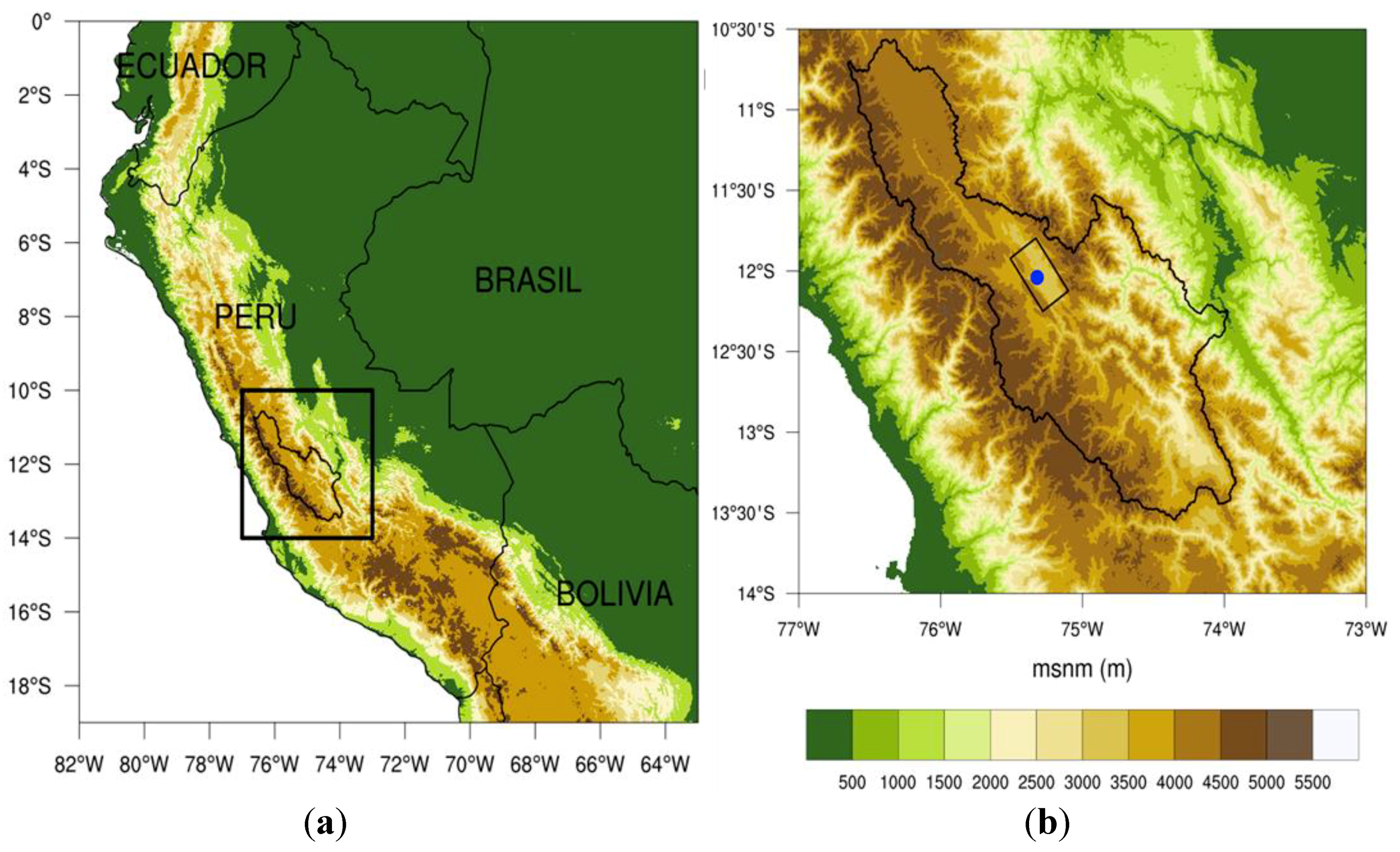
2. Instrumentation and Methodology

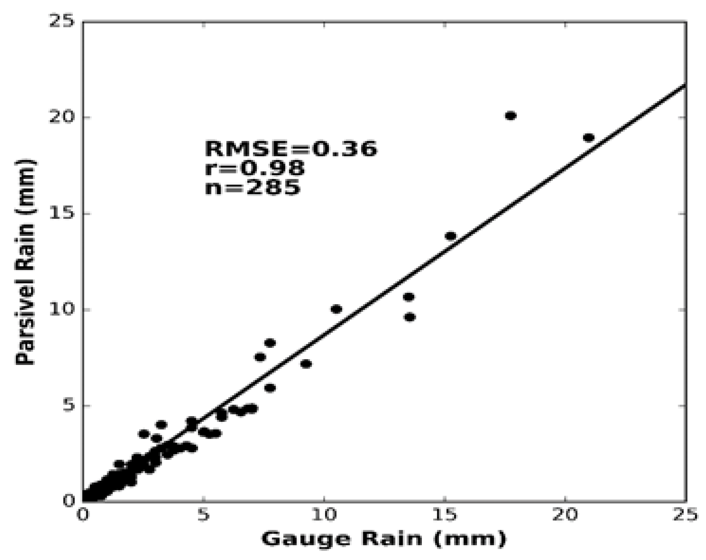
2.1. Parsivel Disdrometer

In this work, the 2nd generation OTT Parsivel disdrometer (Parsivel2) was used. This instrument was introduced in 2011 and underwent a comparison of RSD measurements with the original OTT Parsivel and Joss-Waldvogel (JW) disdrometer at NASA*s Goddard Space Flight Center, Greenbelt (EE.UU). The intercomparison [26] showed that the Parsivel2 gave evidence for consistent and better agreement with the rain gauge than the original OTT Parsivel and JW disdrometer. Consequently, Parsivel2 can be considered to be an improved version of the OTT Parsivel for the measurement of RSD.

Parsivel2 is installed in the Huancayo Observatory (HYO) of the Geophysical Institute of Peru (IGP), as part of the Laboratory for Microphysics and Radiation (LAMAR). The observatory is located at 3350 m above sea level (m.a.s.l) on coordinates 12.04S and 75.32W. Contour lines of the topography of the Mantaro basin and its limits are shown in Figure 1. Parsivel2 receives its name from its property of simultaneously measuring the fall velocity and size of precipitation particles, (PARticle SIze and VELocity), consisting not only of rain, but also including snow, graupel and hail in the most general case [27]. It consists of an optic sensor emitting a beam of laser light with 1 mm thickness, horizontal surface of 180 × 30 mm² (74 cm²) and with a wave length of 780 nm. The size and fall velocity output is expressed in matrix form (32 × 32), where the fall velocity and size of the precipitation particles are classified on intervals from 0.2 to 25 mm/s and from 0.2 to 25 mm respectively. To make statistical computations of the RSD spectrum, the first kind in size (0.062–0.187 mm) is not used because its signal is very low and it is considered to be noise. Figure 2 shows the comparison of rainfall accumulate estimated from Parsivel2 with the tipping-bucket rain gauge, showing some underestimation.

The particles are considered to be approximately spherical for sizes less than 1 mm, as in this case the ratio between longitudinal and lateral axis is considered 1. Instead, for sizes between 1 and 5 mm, a correction is made ($1.075-0.075D_{eq}$) to determine of longitudinal axis, meanwhile for the diameters larger than 5 mm, it is assumed that the ratio between longitudinal and lateral axis is equal to 0.7 (D ≥ 5 mm) [28]. The physical working principle of the Parsivel2 is based on the extinction of the optical beam, since, as the hydrometeors cross the plain laser beam, they generate a shadow that is related with the size of the particle, while the signal duration is used to estimate the velocity of the particles [27].

For to study the cloudiness spatial distribution was estimated from the cloud top brightness temperatures from the Geostationary Operational Environmental Satellite GOES-13 dataset imagery (10.5μm; channel 4), at 30-min intervals and at 4.0 km resolution.

To identify the cloudiness over HYO, including the vertical velocity field, a cloud profiling radar MIRA-35C was used. It is a magnetron-based pulsed Ka-Band Doppler radar, operating at 34.85 GHz (wavelength of 8.6 mm). The radar is directed vertically upwards, allowing registration of the reflectivity and vertical velocity profiles of the cloud and precipitation particles, as they move over it. The radar transmits a linearly polarized signal, receiving simultaneously the scattered Co and Cross polarized components. It can detect cloud and precipitation particles, even if attenuation is an important factor in the case of heavy precipitation [29]. It has a minimum valid height of measurement of 200 m a.g.l, a beam width of 0.6° and high sensitivity. For this study, radar reflectivity (dBZ) was used for cloud detection and, together with the Doppler velocity record (m/s), also to estimate the type of precipitation, while the spectral width (m/s) was used to estimate turbulence.

2.2. Methodology

The Parsivel2 provides the RSD measurements and the fall velocity (V(D)) of hydrometeors. From both data the gamma parameters and integral variables can be calculated as Nw, Dm, Z, LWC, and R. RSD is defined through a normalized gamma function N(D) that represent the raindrop number concentration (per volume and diameter units). This work calculated the gamma parameters and integral variables using N(D) [30,31], as shown in the following equations.

Liquid water content (LWC) [$\frac{g}{c{m}^3}$]:

$$LWC=\frac{\pi {\rho }_w}{6}{{\displaystyle \int }}_{D_{min}}^{D_{max}}N\left(D\right)D^{3}dD$$

(1)

where ${\rho }_w\left[\frac{g}{c{m}^3}\right]$ is the liquid water density.

The mass-weighted mean diameter (Dm) in millimeter:

$$D_m=\frac{{{\displaystyle \int }}_{D_{min}}^{D_{max}}N\left(D\right)D^{4}dD}{{{\displaystyle \int }}_{D_{min}}^{D_{max}}N\left(D\right)D^{3}dD}$$

(2)

Using LWC and Dm, the intercept parameter (Nw)($m{m}^{-1}{m}^{-3}$) is obtained by

$$N_w=\frac{4^4}{\pi {\rho }_w}\left(\frac{LWC}{D_m{}^4}\right)$$

(3)

Thus, the total concentration (Nt) is obtained as

$$Nt={{\displaystyle \int }}_{D_{min}}^{D_{max}}N\left(D\right)dD$$

(4)

Likewise, R is obtained using N(D) and V(D):

$$R=\frac{6\pi }{{10}^4}{{\displaystyle \int }}_{D_{min}}^{D_{max}}N\left(D\right)V\left(D\right)D^{3}dD$$

(5)

The fall velocity is calculated as a function of raindrop size from an empirical equation proposed by [32,33].

$$v_f\left(D,h\right)=9.23\left[1-exp\left(-0.068D^2-0.488D\right)\right]{\left(\frac{{\varphi }_o}{\varphi \left(h\right)}\right)}^{0.45}$$

(6)

where $v_f$ is the fall velocity, ${\varphi }_o$ is the air density at mean sea level (m.s.a.l), ϕ(h) is the air density as a function of height h and D is the raindrop diameter.

The convective and stratiform clouds are clearly distinguished by the vertical velocity. The microphysics of both rainfall are different, as the evolution of the cloud hydrometeors depends on the vertical draft velocity in the cloud [34]. In convective clouds, the microphysical processes such as freezing and riming, occur when updrafts carry liquid hydrometers above the freezing level, while in stratiform rain, the aggregation and deposition are that occur in an environment of slow ascent is predominant in the growth of hydrometers [35,36]. As the accurate measurement of vertical velocity in precipitating clouds is complex, observations of this parameter are generally not available, and so, disdrometer and radar estimations, based on reflectivity, were used to study the distribution and characteristics of the two types of precipitation.

In the Central Andes of Peru, liquid, solid, and mixed phase precipitation occur. To evaluate the impact of this precipitation on the agriculture, water supply and infrastructure, it is necessary to evaluate not only the accumulated rainfall, but also the daily cycle of rainfall rate, the type of precipitation, the phase composition, and the raindrop (or particle) size distribution RSD. The objective of the present study is to analyze the spectral distribution of RSD for different rainfall regimes, including convective and stratiform rain events. To study the diurnal cycle of the RSD, a specific classification was applied, so that each rainfall rate class contributes in one third to the total accumulated rainfall. The discrimination of rainfall as convective or stratiform was attempted using Parsivel2. The methodology of [12] is applied with slight variations. This consists of establishing a threshold value of R to define convective rainfall, so that in a time series of R values, at time interval k, the $R_k$ and the eight adjacent values (from $R_{k-4}$ to $R_{k+4}$) must be less than 10 mm/h, for considering the k spectrum as stratiform rainfall; otherwise, k spectrum is classified as convective. A criterion using the reflectivity is also applied, so that intense cells with reflectivity Z > 38 dBZ are considered to be convective rainfall, and otherwise they are classified as stratiform [35,37,38]. This classification using the combination of thresholds (Z and R) has certain limitations to distinguish weak or edge of convection from stratiform. However, in most cases it is very useful to discern individual events of stratiform and convective rain. Before the application of the statistical technique to the data recorded by the disdrometer, the rain events were identified. The methodology considers a rain event duration threshold value of eight consecutive minutes, and an accumulated rainfall threshold minimum value of 2 mm. Once a rain event was identified by this criteria, then it is classified as convective or stratiform by the previously mentioned methodology. In the present paper, rainfall was treated considering rain events, as defined above, which by definition, excludes part of the one-minute rainfall samples, and also considering all the rainfall samples.

3. Results and Discussion

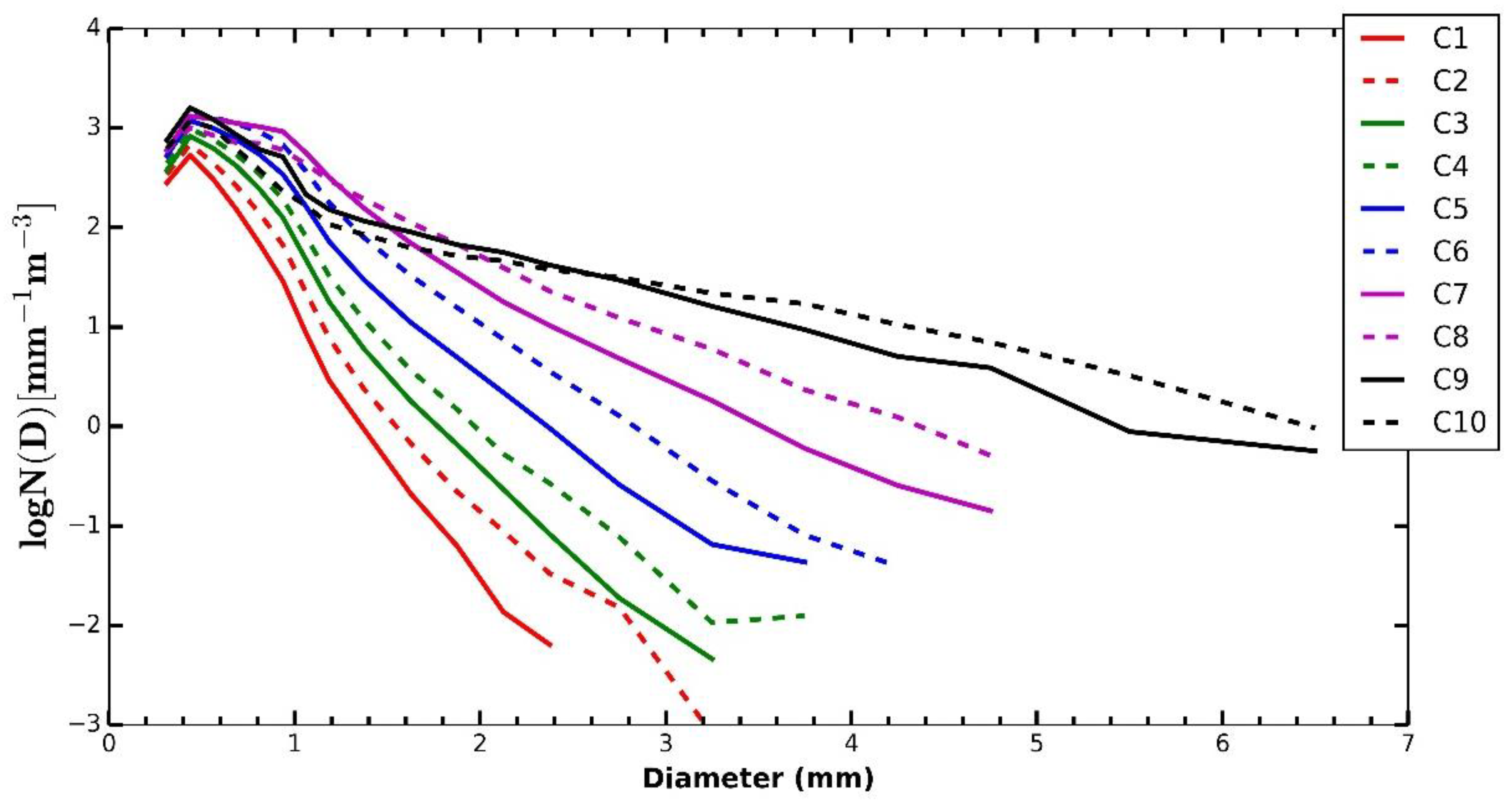
3.1. Raindrop Size Distribution

Table 1. Characteristics of the raindrops size distribution (RSD) in function of the rain rate class; number of cases (n) in each minute, rain rate (R [mm/h]), liquid water content (LWC[g/m3]), concentration total number (Nt [1/m³]), mass-weighted mean diameter (Dm [mm]), intercept parameter (Nw [1/(mm m³)]). These variables were calculated for a period of 18 months between 2017 and 2019 registered by Parsivel2.

Class	n	R	LWC	Nt	Dm	Nw
C1(0.1–0.2)	3912	0.1	0.02	173	0.70	3.73
C2(0.2–0.4)	6203	0.3	0.03	247	0.77	3.81
C3(0.4–0.7)	5503	0.5	0.05	337	0.84	3.89
C4(0.7–1.0)	3383	0.8	0.07	428	0.91	3.91
C5(1.0–3.0)	8037	1.5	0.12	587	1.05	3.92
C6(3.0–6.0)	2070	3.6	0.25	851	1.22	3.97
C7(6.0–10)	452	6.9	0.44	968	1.55	3.79
C8(10–20)	206	11.6	0.63	772	2.10	3.43
C9(20–40)	87	28.4	1.24	867	3.27	2.95
C10(40–120)	36	51.7	1.76	658	3.89	2.80

shows the RSD characteristics and its parameters, following the classification of the rainfall rate (R) in the interval from 0.1 mm/h to 120 mm/h. In this way, all the records are categorized in 10 classes (C1, C2, C3, C4, C5, C6, C7, C8, C9 and C10). R and the liquid water content (LWC) were integrated using the averaged spectra and the fall velocity of the drops for each category. These values are consistent with the expected potential dependence of LWC with R. The total raindrop concentration Nt increases with classes intensity till C7; For classes C8, C9 and C10 there is no marked trend. Dm increases with classes intensity. Instead, Nw, expressed in logarithmic scale, varies only slightly in all classes. In Figure 3, high concentration can be noticed for small diameters (around 0.5 mm), which shows the abundance of small raindrops for all kinds of rain and the partial concavity under of 0.27 mm is probably related to lack of small drops due to the dead time problem of the Parsivel disdrometer [38]. The average spectrum is clearly different for every kind of rainfall event (Figure 3), so that for lower intensities, the spectrum rapidly decays with diameter, while the spectral value for a given diameter increases with rainfall rate, so that the slope of the spectral curve decreases with rainfall rate class, as expected. On the other hand, average spectra for classes C9 and C10, which have fewer cases, present particular characteristics, reaching high values for diameters as large as 6.5 mm. This can be related with an efficient collision-coalescence process or can also be the result of melted or partially melted hail. The most frequent values of R observed in the valley lay in the range from 0.1 mm/h to 6 mm/h, wherein, Nw and Nt increase with R. For rain intensities greater than 6 mm/h, the rain events are considered to be extremes, as their occurrence lays within the 95th percentile the record, corresponding R > 4.3mm/h. Rainfall rates greater than class C6 represent 3% of occurrence.

The classification of rainfall in 10 classes was made for the whole dataset without considering the time of occurrence. However, one of the purposes of the present investigation is to understand the diurnal variation of the rain spectrum. Consequently, the frequency of occurrence of rainfall events in local time intervals (15–20, 21–02, 03–08 and 09–14 local standard time (LST)) was evaluated, considering three wider classes of events: light rainfall (L), moderate rainfall (M) and heavy rainfall (H) for those time intervals. In this case, the classification was carried out in a different way, so that each type of rainfall contributes in one third to the total accumulated rainfall.

It must be noticed that the rainfall classification was made only for the wet season (November–April) that approximately contributed 82.93% to the total yearly accumulated rainfall (826.52 mm). The South America Monsoon system of (SAMS) conditions very definite seasons regarding precipitation, particularly in the Central Andes [39]. Precipitation in the Andes mainly occurs during the austral summer linked to the mature phase of SAMS. During this period, more convective precipitation occurs, and total accumulated rainfall is also greater, while in the winter, precipitation events are very scarce. This was the reason to limit the analysis period. The diurnal average variations of RSD of each type of rainfall (L, M, H) is shown in Figure 4. It is clearly observed that the RSD spectrum is different for the three types of rainfall events. The general dependence of the form of the spectra and the spectral values with rainfall rate class is independent of time of day, as the for all the intervals the slope of the spectrum decreases with rainfall rate, but it can be noticed that the largest diameters are reached in the time interval (15–20 LST), corresponding to the time of maximum development of convection, where hailstorms occur in the valley [22,23,40]. In the morning and early afternoon (09–14 LST) also occur spectra with large raindrops in the high rainfall rate class, corresponding to early developing storms that can also produce hail in some cases. For the late night (21–02 LST) and early morning (03–08 LST), the spectra are quite similar, even if in the late night ones, the maximum diameters are larger for the three classes. On the other hand, all the spectral curves show a maximum in D = 4 mm, and the dependence of the average spectra on rainfall rate class for smaller diameters is weak.

Considering all the one-minute samples, most of the accumulated rainfall (49%) belongs to the 15–20 LST, interval. The corresponding spectra show the highest maximum diameters and maximum concentrations for each diameter range (Figure 4).

Table 2. Diurnal cycle of the contributions of one-minute rainfall samples to total rainfall registered by Parsivel2. In 6-h intervals, including all the one-minute measurements (November–April, in total 12 months of the 2017–2019 period) of the heavy and moderate rain. The parentheses indicate contribution in percentages. H: heavy events M: moderate events.

Hours during the Day	15–20 LST		21–02 LST		03–08 LST		09–14 LST
Contribution to rainfall (mm)	334.6 (49%)		201.8 (29%)		88.2(13%)		60.8(9%)
Time of duration (minutes)	17952		13594		8340		5268
Classes of events	M	H	M	H	M	H	M	H
Contribution (%)	29	46	42	22	36	15	24	35

summarizes the contribution to the accumulated rain (mm) of each of the 6-h intervals of the diurnal cycle and includes the total rain duration in minutes in each of the time intervals during the wet season. It also includes (in parenthesis), the contribution in percentage of the classes of events according to the defined time intervals. For example, in the 15–02 LST interval, the moderate class rain (M) contributed 29%, the heavy class rain (H) contributed 46%, while 25% corresponds to the light class contribution (L). (not included in the table). It can be noticed that most precipitation occurs in the (15–02 LST) interval.

Figure 5 shows the distribution functions of the normalized RSD parameters for each of the defined time intervals. The Dm distributions present generally two modes throughout the day. In the heavy rain case (H), its greatest main mode occurs on the 15–20 LST period, decreasing gradually in the subsequent periods, consistently with the maximum drop growth at the maximum convection period. This also holds for moderate rainfall, with maximum modal diameter at the maximum convection period, even if the dependence in the rest of the diurnal cycle case is not so marked for this case. On the other hand, modal Dm for the light rain cases shows no significant diurnal cycle. The distributions of Nw show a weak diurnal variability. In the M and H categories, Nw has a tail in larger concentrations that is most prominent during the daytime and early evening when convection is active. The prominence of the large Nw tail is more during the day including mid-morning to early afternoon and early afternoon to late afternoon. The Nw tail begins to weaken during evening hours and disappears by the end of the night (late evening to early morning).

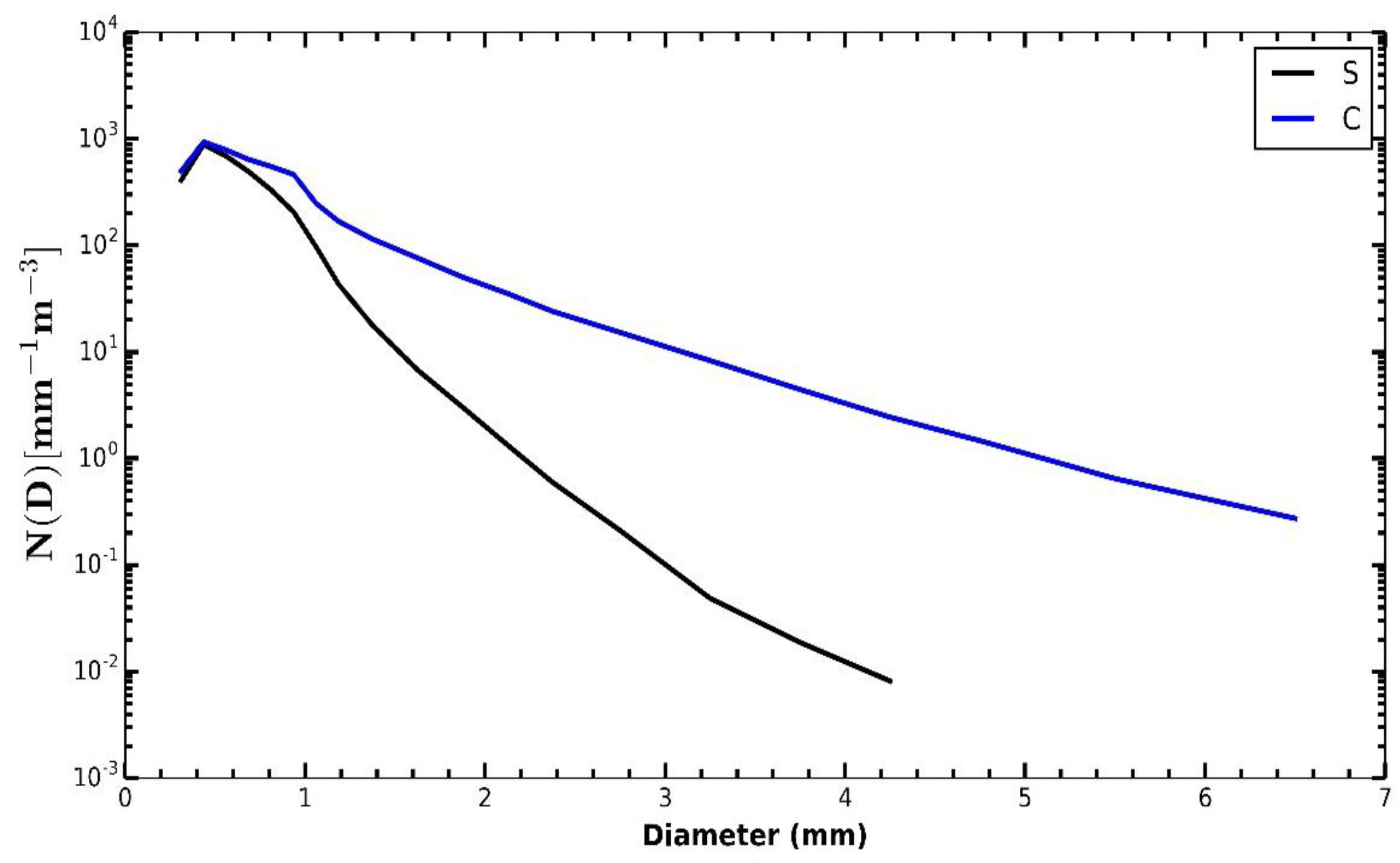
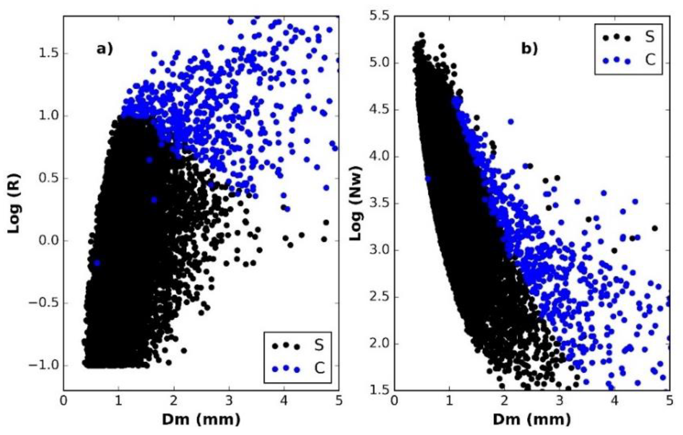
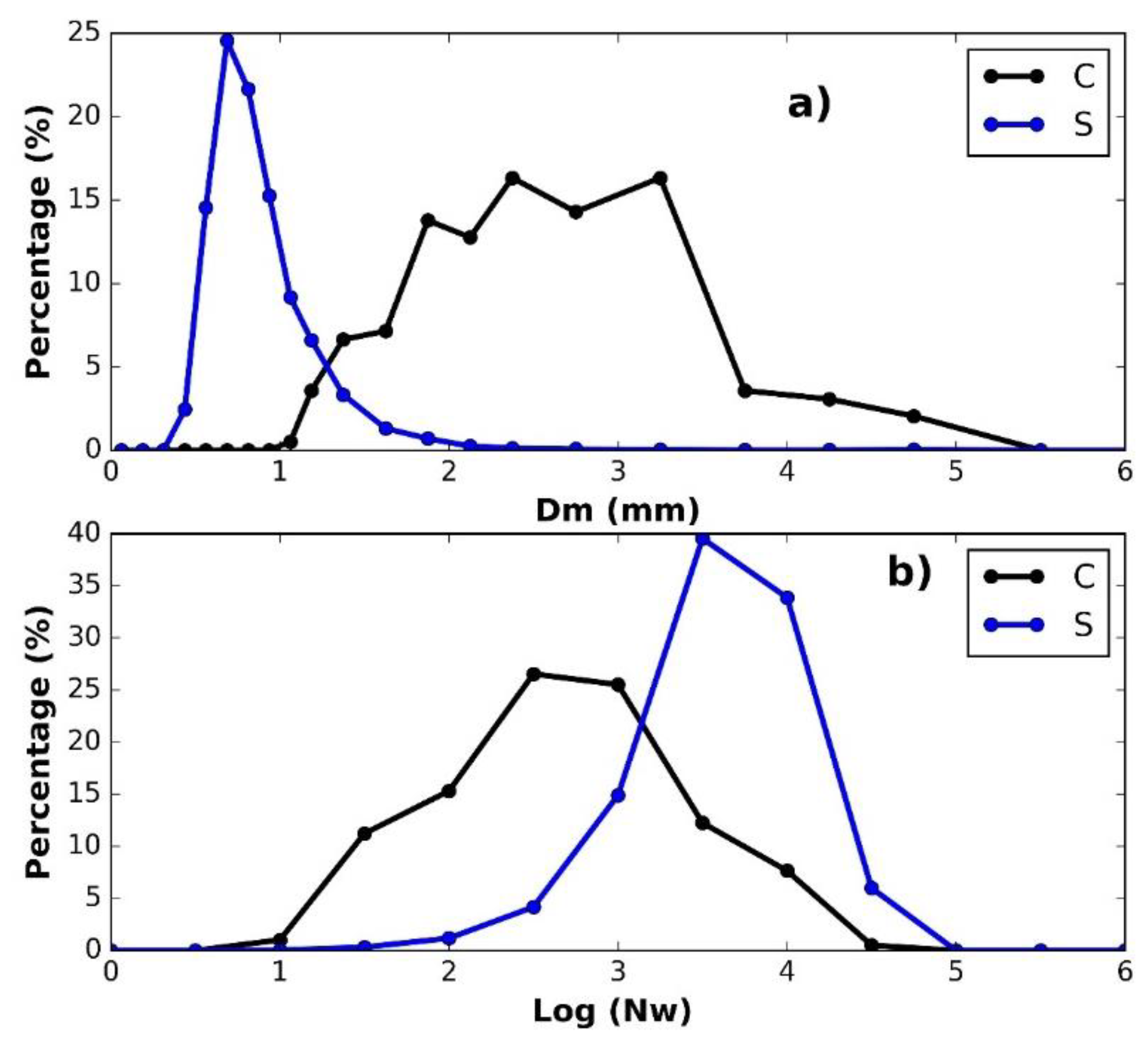
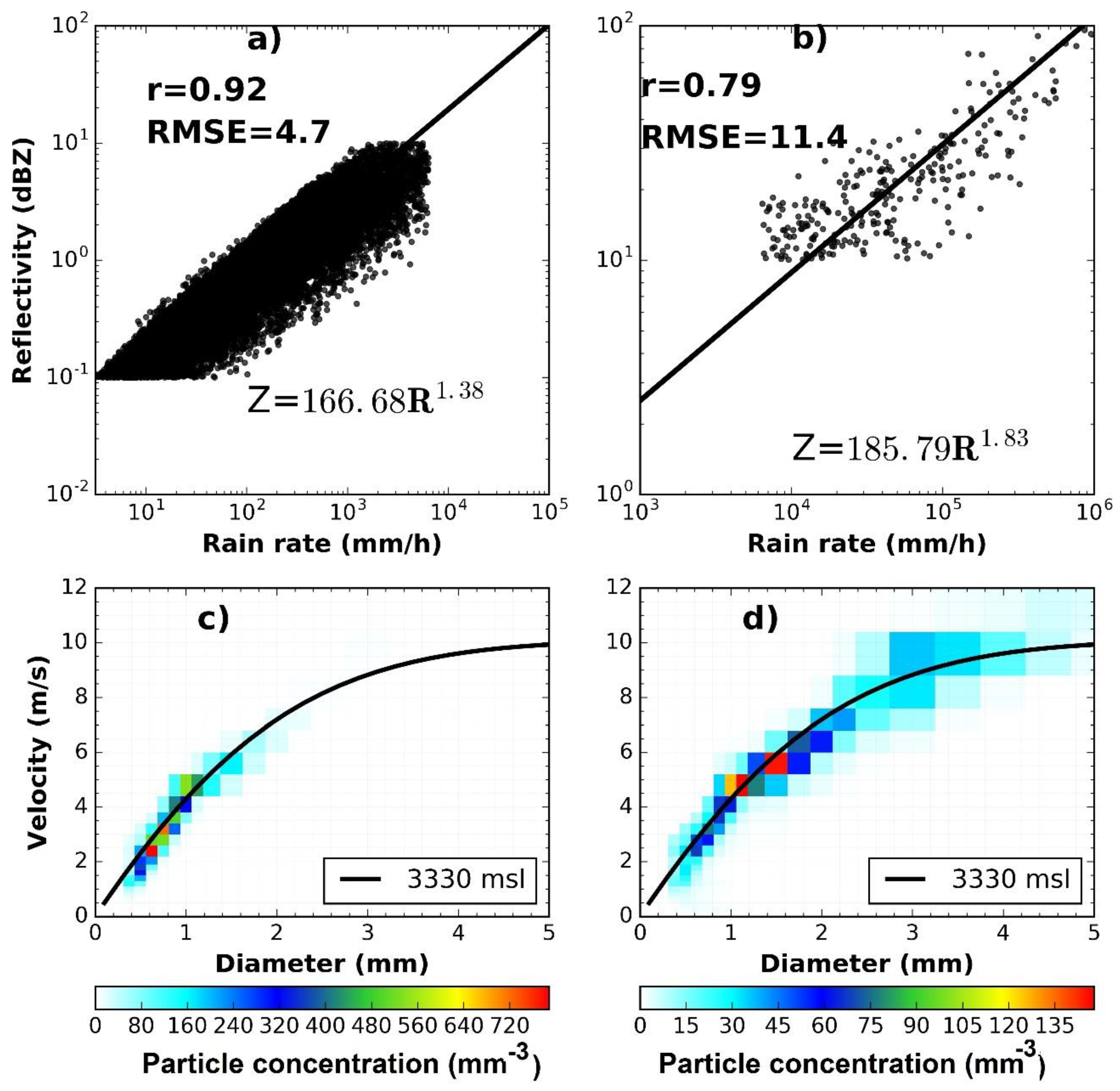
3.2. Convective and Stratiform Rainfall

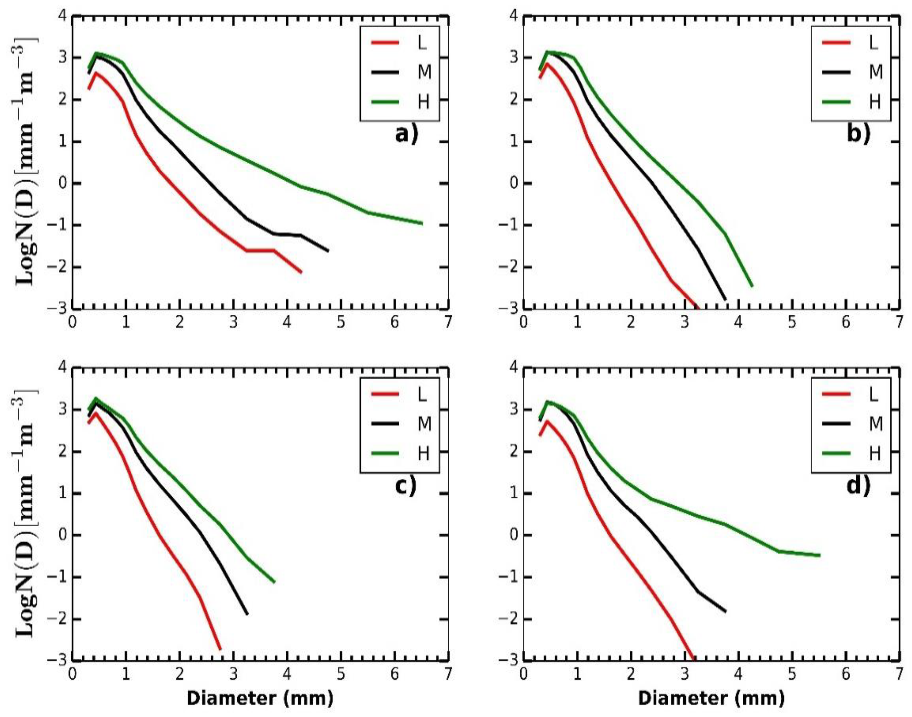
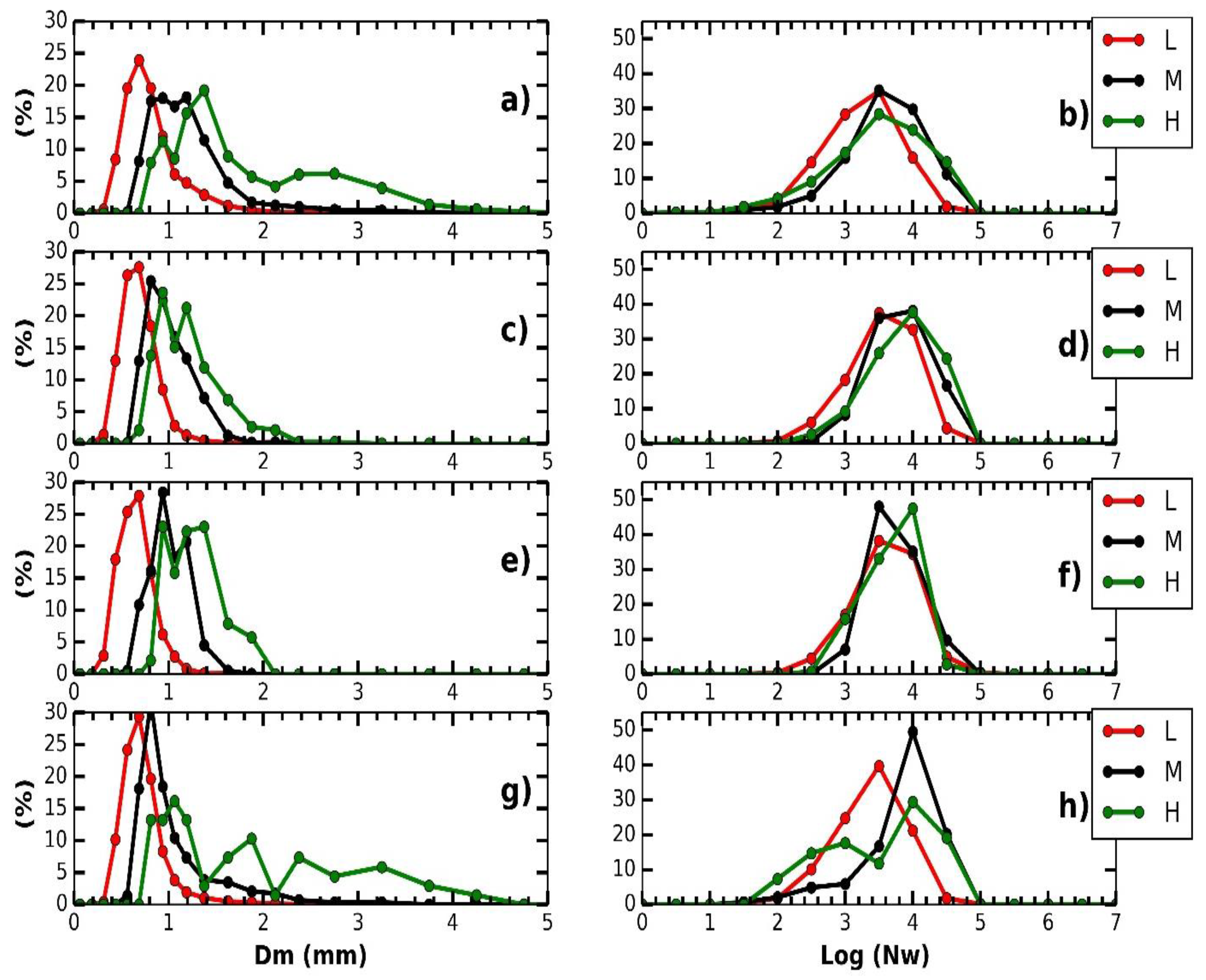
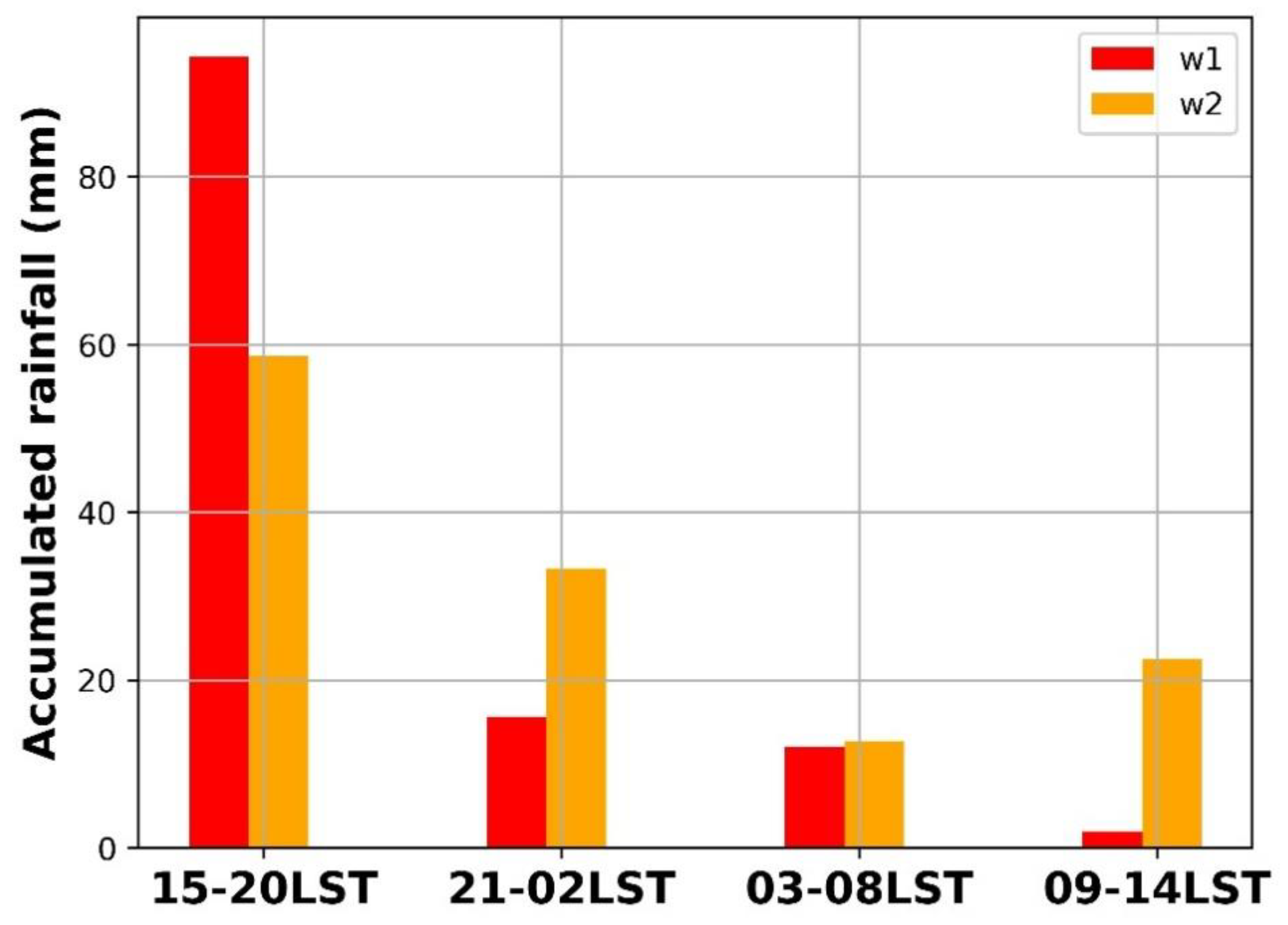
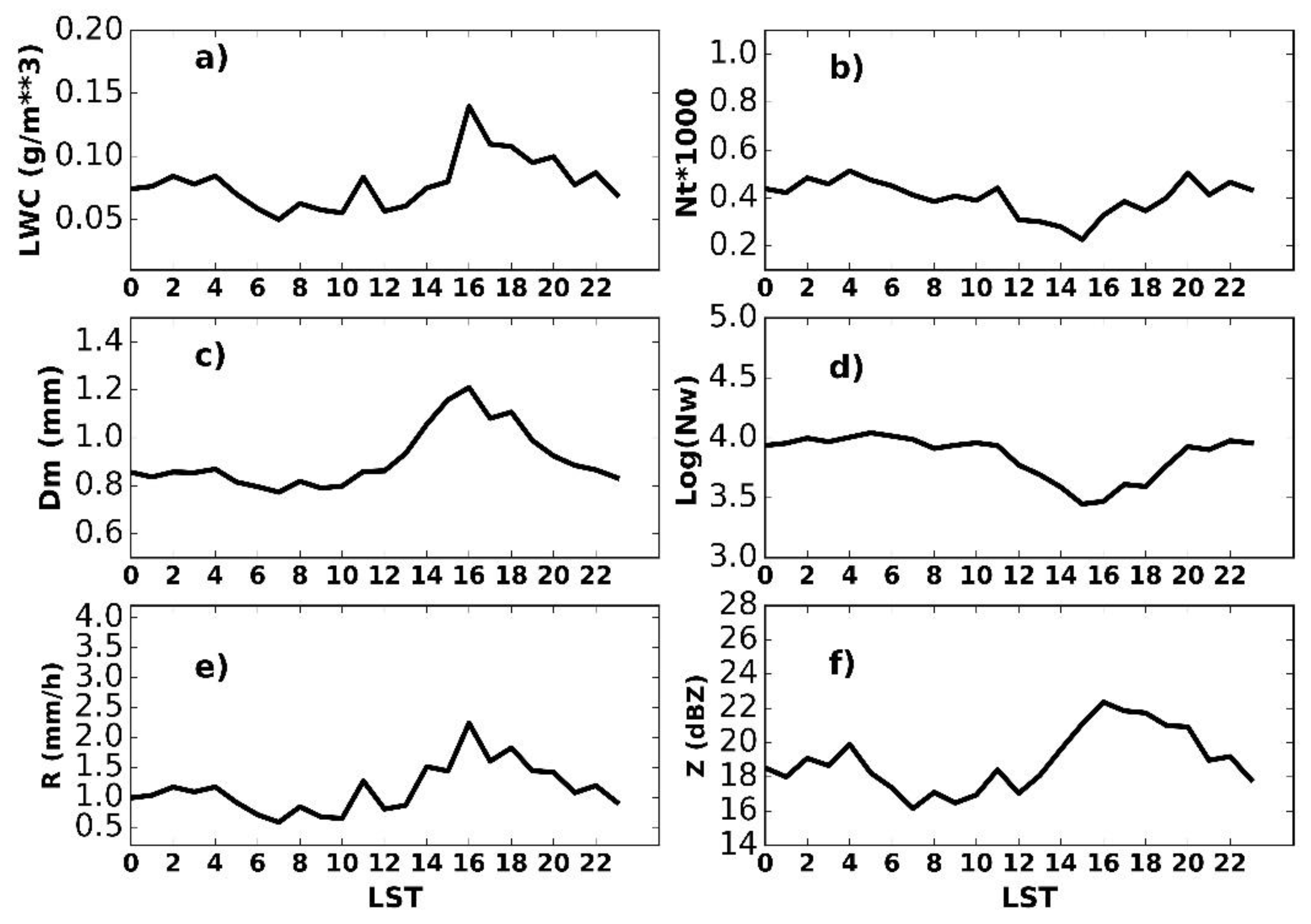
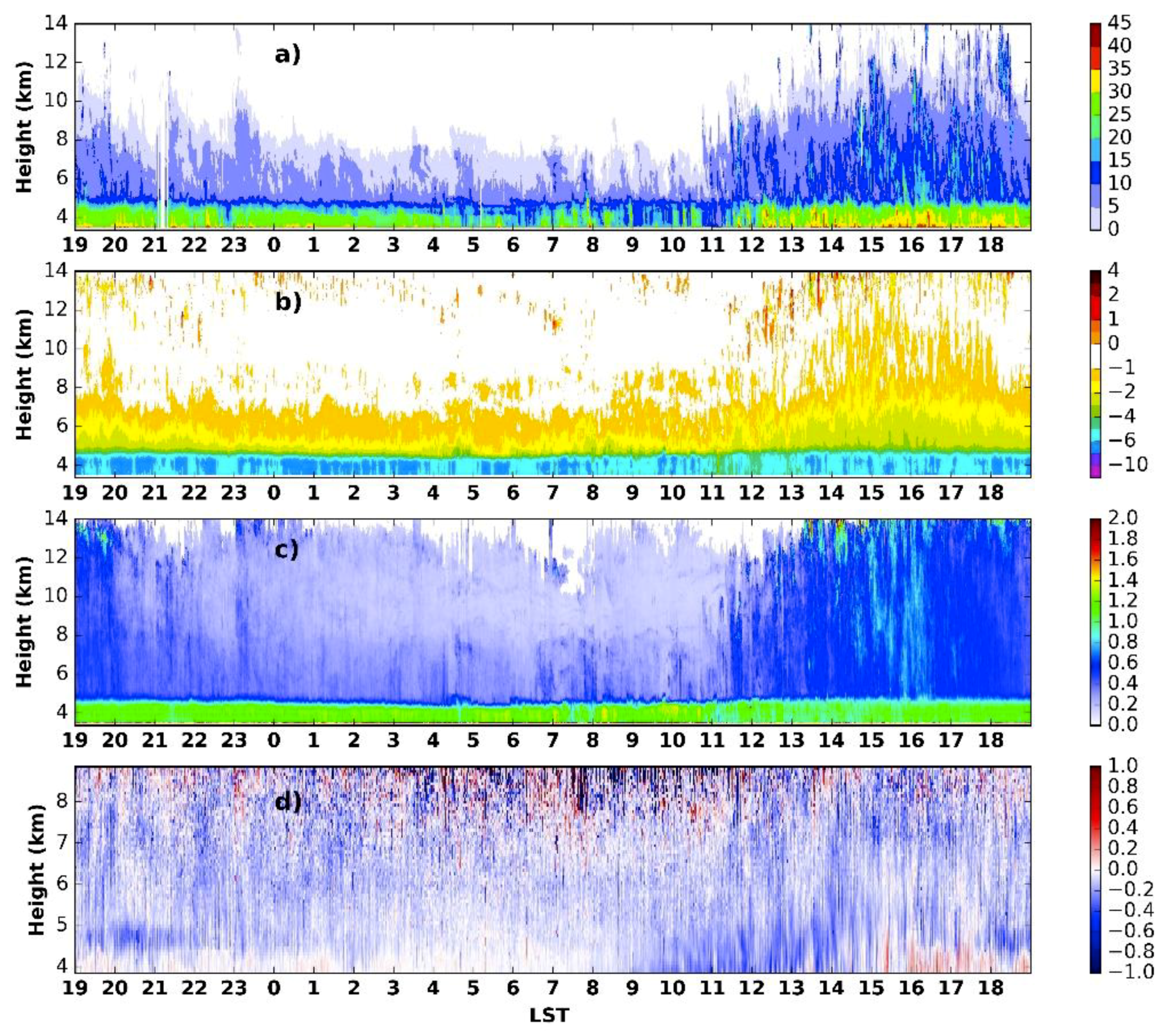
From the definition of rain event and of convective and stratiform rain used in this paper, described above in Section 2.2, it follows that a rain event can contain convective and stratiform rain periods, consistently with the simultaneous presence of a convective core and stratiform rain from the anvil in thunderstorms [9,35]. According to the methodology of classification, based on rainfall rate and reflectivity values in the time series of the Parsivel2 record (Section 2.2), 18 rain periods were labeled as convective (C, which in general, are associated with cumulus or cumulonimbus clouds and occur in the afternoon, while the rest are classified as stratiform (S). The date and time of occurrence of rainfall events containing convective rainfall is shown in

Table 3. Date and time of occurrence of the rainfall events containing at least 10 min of convective rainfall in a sample of 18 months, between 2017 and 2019 with Parsivel2 records. S is the time (minutes) duration of the stratiform rainfall in every event and C is the time (minutes) duration of the convective rainfall in every event. $D{m}_{max}$ is the maximum diameter (mm) and $R_{max}$ is the maximum rain rate (mm/h) of the rainfall event.

N°	Date	C	S	$\mathit{D}{\mathit{m}}_{\mathit{m}\mathit{a}\mathit{x}}$	${\mathit{R}}_{\mathit{m}\mathit{a}\mathit{x}}$
1	20171015 12:38	10	48	2.3	24.4
2	20171223 16:09	22	29	4.6	46.8
3	20180111 17:50	37	94	4.0	76.2
4	20180113 15:53	10	4	5.4	23.5
5	20180117 19:47	15	63	1.7	31.5
6	20180118 18:31	14	16	2.3	32.1
7	20180209 15:40	10	55	3.1	21.5
8	20180217 19:29	15	18	3.0	30.8
9	20180221 15:40	10	13	5.3	32.2
10	20180221 16:04	10	148	1.6	11.5
11	20180226 18:52	16	36	5.5	16.6
12	20180807 14:50	16	30	5.8	52.6
13	20180915 16:20	33	22	5.3	96.0
14	20181115 17:58	15	135	3.9	90.6
15	20190307 14:26	18	15	4.6	43.3
16	20190402 11:14	10	88	2.6	32.8
17	20190403 14:53	10	15	3.7	37.6
18	20190410 14:36	13	23	5.4	58.1

. These events containing convective rain are of special importance to understand more about the dominating physical processes in these phenomena. Their frequency of occurrence is low, but they are very important, because of the possible occurrence of hail, which can entail a hazard for crops and installations, causing a negative economic and social impact. The averaged characteristics of the integral parameters of individual DSDs, divided in C and S types are shown in

Table 4. Averaged gamma parameters and integral variables calculated for convective (C) and stratiform (S) rains from the RSD dataset between 2017 and 2019 where n is the number of individual samples for each type of rain.

Class	n	R	LWC	Nt	Dm	Nw
C	565	13.6	0.7	630	2.98	3.73
S	31649	0.8	0.08	402	1.04	2.88

. The number of occurrence of stratiform rains is larger than the convective ones, but the averaged integral parameters; R, LWC, Dm and Nw are much larger in the convective rain.

The averaged spectra for the two types of rains are clearly different (Figure 6). The main characteristics of the spectrum of convective clouds (C) relative to the one for stratiform clouds (S) are its lower slope to the right of the maximum and its greater maximum diameter. The first evidence the prevalence of the microphysical processes; that could it be melting of graupel, small hail and the presence of active condensation-coalescence processes that guarantee higher concentrations of raindrops of large diameters.

It can be noticed that the concentration of small drops, with diameters of less than 0.5 mm, is similar for convective and stratiform clouds. These results are different from the observations of [41] in Guyuan-China, where the concentration of small drops was greater for stratiform rain. In the Guyuan case, the climate is continental temperate dry, while in the Mantaro valley, the humidity high and the cloud base is relatively near to the surface, so that the evaporation rate is small, both for stratiform and convective rain. On the other hand, the frequency of occurrence of C in the Mantaro valley is less (565 samples) than S (31,649 samples),and both Nt and LWC are greater for C than for S. Normalized parameters of the gamma function are different too, so that Nw parameter for C (3.73) is smaller than for S (2.88).

The scattering diagrams of the classic and normalized RSD gamma distribution parameters were used as a criterion for discerning convective and stratiform rain events, as the points of each type of rainfall generally cluster in different areas of such a diagram. [14] used a No vs. R diagram for a classic gamma distribution fit, and [12] extended this method to a normalized gamma distribution. In this paper, the normalization developed by [42] was applied, and scatter diagrams of log10(R) vs. Dm and log10 (Nw) vs. Dm were showing the separation of the points corresponding to types C and S (Figure 7). This result shows that there is a clear distinction between both types of precipitation (C and S). In stratiform rainfall, Dm values are small and middle, occupying predominantly the left and lower area of the log10(R) vs. Dm plot in Figure 7a, while the convective rainfall points occupy the upper right area. The scatterplot of Figure 7b (log(Nw) vs. Dm) shows an even clearer separation between C and S rainfall observations, showing that the relationship between R or Nw and Dm can be a good criterion to estimate the type of rain. Figure 8 shows the percentage of occurrence of the RSD parameters across types of precipitation. The type C rain events have one mode, but it is a broad mode between 1.5 and 3.2 mm. Instead, in the type S precipitation is present one narrower mode, whose peak is centered around 0.8 mm. Similarly, the distributions of the Nw parameter are unimodal for C y S rains.

Figure 9 shows the dependence of reflectivity on rainfall rate (a, b) and of fall velocity on diameter (c, d) for the rain events over the valley for the two rainfall types. The left panels refer to stratiform rain and the right panels to convective rain.

The Z–R relationship (Figure 9a,b) depends on the RSD, which is a consequence of microphysical processes involved in rain formation, which are related with the type of cloud, and regional, orographic, and seasonal factors [6]. It is expressed by an empirical equation (Z = aR^b) where a and b are parameters which can be derived from the RSD [5]. The scatterplots and regression line of log(R) vs. log(Z) are shown in Figure 9. The convective rainfall presents a relatively low correlation coefficient (r = 0.79) and the root mean square error (RMSE) is large, as a consequence of the highest spatial and temporal variability of this type of rain. Meanwhile the stratiform rainfall has a high coefficient (r = 0.92) and a low RMSE (4.7), allowing a more precise estimate of the Z-R relationship parameters (a = 166.68 and b = 1.38), due to the more uniform behavior and higher frequency of occurrence of these type of rain.

Regarding fall velocity, significant concentration values for stratiform rain (Figure 9c) are grouped in the 0.7–6 m/s interval, wherein the higher values are between 0.5 and 1 mm. Meanwhile, the fall velocity of convective rainfall is grouped in the 2–12 m/s interval and mainly in the interval 1–2.5 mm. Both results are consistent with the RSD average shown in Figure 6 and also with previous studies [41]. On the other hand, the black line indicates the curve obtained using Equation 6. [32] and [33], considering air density at 3330 amsl (HYO position). This curve approximately fits the Parsivel2 data, so that in general terms, its application is reliable for rainfall estimation through remote sensing (cloud and rainfall radars) in Andean areas. The fall velocity values for stratiform rain (Figure 9c) are grouped in the 0.7–6 m/s interval, wherein the higher values are between 0.5 and 1 mm. Meanwhile, the fall velocity of convective rainfall (Figure 9d) is grouped in the 2–12 m/s interval and mainly in the interval 1–2.5 mm. Both results are consistent with the RSD average shown in Figure 6 and also with previous studies [41].

3.3. Diurnal Cycle

The rainfall events containing convective rainfall (RCC) contributed 235.2 mm to total accumulated rain, representing the 34.3%, from which the convective rainfall represents the 8% and stratiform rain the 92%. Particularly in the 15–20 LST interval, the RCC contributed 172.2 mm to the accumulated rain, equivalent to the 73% of the total rainfall. Figure 10 shows the diurnal cycle of the accumulated rainfall from RCC, for the rainy (wet) seasons of 2017–2018, denoted by W1 (31 events in 6 months) and 2018–2019, denoted by W2 (30 events in 6 months). The relative contribution of the two types of rainfall in both seasons is clearly different, as in W1, the occurrence of convective and stratiform rain lasted 250 and 1559 min. respectively, whereas in W2, the convective and stratiform rain periods were 196 and 2111.min., respectively. It was also observed a difference in the diurnal cycle for the two seasons. In both cases, the rainfall contribution decreases from the 15:20 to 03:08 LST periods, but in the case of W2, morning rainfall was greater than in the night. This suggests that for W1, the convective rainfall, which developed practically only in the afternoon, at the time of maximum solar radiation, produced most rainfall in the mature stage of convective storms and gradually decayed afterwards, giving more stratiform rainfall from the anvil clouds. In the case of W2, a secondary maximum is observed in the morning hours, indicating an early development of convection. A significant difference in the 15–20 LST contribution is also observed between W1 and W2, so that W1 contributed ~62% of the total RCC rainfall in the total 12 month sample. In contrast, in season W2, the 21–02 LST and 09–14 LST intervals contributed more than W1 by 69% and 98% respectively. From previous studies [19,43] it is known that there is a strong correlation between El Niño Southern Oscillation (ENSO, preferably with the Niño 4 index) and rainfall during the peak phase of the rainy season in the Mantaro basin, so that this relationship particularly indicates a background effect on the rain of Mantaro valley. Therefore, the variation of the diurnal cycle and the deficit of convective rainfall in W2 season is very likely associated with the occurrence of the El Niño phenomenon. This suggests a possible influence of El Niño event in the mechanisms of convective rain development in the Central Andes that should be investigated using a longer record of convective rain, including several of these events.

Figure 11 shows the diurnal cycle of the average of six RSD integral parameters. In the cases of LWC, Z, R and Dm, a single mode is found, within the interval 15–18 LST with maximum peak at 15–16 LST. For the same interval, the concentration parameter (Nw) and the total number of particles (Nt) decrease significantly, probably because of the presence of precipitating convective clouds during this time, with the possibility of melting, coalescence, and riming processes so that the growth of large drops is intensified, as shown in Figure 11c. The cloud radar (Mira35C) observations confirm this result, as the observed reflectivity by the cloud radar (Figure 12a) coincides adequately with the single mode of the integral parameters. During the time interval of high value of the integral parameters (15–18 LST), The reflectivity record reaches high levels, but most of the larger Z values are mostly confined to regions below the melting level. This is mainly related with the strong attenuation that is characteristic of the relatively short wavelength in the presence of intense convective rainfall. Therefore Z values show few locations that might be large enough for graupel in the mixed phase zone. On the other hand, in 15–18 LST interval, the Doppler velocity record (Figure 12b) shows peak vertical motions, consistently with the prevalence of stratiform rain in most of the record, as shown in Table 4. The vertical wind velocity positive values (Figure 12d) are associated with cumulus convection. Instead, during the early morning, the opposite occurs, and the down and slow vertical motion predominate. In addition, the spectral width physically represents the turbulence that occurs within the structure of precipitation clouds, so that high values of spectral width indicate the occurrence of intense turbulence, coincident with the time interval when convection occurs. From these results, we concluded that in the afternoon hours, more active convective clouds are observed, with active raindrop growth and intensification of precipitation processes (Table 3). In contrast, during the late night and early morning (23–06 LST), the raindrops have small diameters, with the presence of downdrafts close to zero. The spectral width parameter is uniform and relatively small with the presence of shallow clouds in the sky and in consequence, during these hours the precipitation is mainly stratiform.

Figure 13 shows the hourly mean of brightness temperature for austral summer. At 11 (Figure 13a) and 12 LST (Figure 13b), cold clouds are observed in the east side of the Mantaro valley. Meanwhile, warm clouds predominate above the west side at the same time. In the afternoon (from 13 LST), the clouds move towards the east and deep cold-topped clouds appear in the west side, probably associated with the incoming moisture fluxes from the Pacific Ocean that enter the Mantaro valley until approximately 18 LST (Figure 12h). At the same time, moisture fluxes from the Amazon basin enter through the east side of the Mantaro valley and generate intense cloudiness from 15 to 17 LST (Figure 13e,f). Probably, the interaction between moisture fluxes coming from the west side (Pacific Ocean) and the east side (Amazon basin) of the Mantaro valley generates intense convective activity associated with the occurrence of thunderstorms and heavy rains as in the case studies discussed by [22,25]. This dynamic process coincides with the decay of the direct effect of solar radiation. Instead, during the night, the dynamics of the clouds behaves differently. Storm clouds developed above the Amazon basin, (Figure 14) and due to the anticyclone circulations at mid and upper levels of the atmosphere, these cloud systems strongly influence the rains occurring in areas of the Central Andes. In general, the rains that are registered in the Mantaro valley are fed mainly by those two sources; one on the north side of the valley and the other on the south side (Figure 14b,e,f,g) which means that the moisture fluxes that enter mainly through these two regions play a fundamental role in the rains that are registered inside the valley, as pointed out by [44].

Figure 15 shows the empirical orthogonal functions (EOFs) of the mean brightness temperature during the southern summer for the period 2010–2017. The first mode (Figure 15a) represents 77.75% of the total. This spatial pattern explains that the Andes mountains influence the variability of the cloudiness, exerting a barrier effect that prevents the entry of moisture fluxes from the Amazon basin, this affirmation is consistent with the study of [23]. As a result of this blocking, two predominant cloudiness regions are formed: the northern cloudiness (NC) and the eastern cloudiness (EC). These regions show cold brightness temperatures, with high concentration of cloudiness associated with deep convection. This spatial pattern occurs during night hours in the interval 1900–1100 LST. During this time the precipitation registered in the HYO is strongly influenced by the configuration of the two regions NC and EC.

The second mode of the EOF shows an important signal which represents 13.29% of the total variance (Figure 15b). This spatial pattern shows the dynamics of the cloudiness that presents a large amount of cloudiness along the Andes cordillera (AC) and on the opposite side the North-East cloudiness (CC). This configuration with cloudiness regions CC and AC is present during the daytime (Figure 13) when the flows of the Pacific Ocean pass over the mountain range and interact with the moist flows from the Amazon over the Mantaro valley [22,25,44]. Therefore, the convective rains mentioned in Table 3 depend mostly on the configuration of the AC and CC regions.

4. Summary and Conclusions

Raindrop size distributions in the Mantaro valley of the Central Andes of Peru, were investigated using 18 months of drop size and fall velocity data from a Parsivel Disdrometer located in the Huancayo Observatory during (2017–2019). From these measurements, gamma distribution and integral rainfall parameters were determined for different rainfall events and rainfall rate categories. The main estimated rainfall parameters were the reflectivity factor (Z), rainfall rate (R), liquid water content (LWC), total concentration (Nt) and gamma distribution parameters Dm and Nw. On the other hand, to understand the spatial dynamics of cloudiness GOES imagery datasets were used and the radar Mira35C for to investigate the cloudiness in the vertical passing over the observatory.

Rainfalls were classified by their intensity in 10 categories (C1, C2, C3, …, C10). For less intense rainfalls, high raindrop concentrations were found, especially of small particles that do not exceed Dm = 1.22 mm. The slope of the spectral curve decreases with rainfall rate class. Average spectra for the higher rainfall rate categories, C9 and C10, reach high values for diameters (6.5 mm).

The diurnal cycle of parameters (LWC, Z, R, and Dm) present one marked maximum in the 14–20 LST interval, in this time interval, when the total concentration and intercept parameter significantly decrease, while deep and more active clouds appear with presence of turbulence. Regarding the form of the spectra, in the 15–20 LST interval, average RSDs have greater slopes than for other time intervals. The presence of diameters larger than 6.5 mm in some of the RSDs can be can also be the result of the presence melted or partially melted hail or can also be a consequence of a particularly efficient collision-coalescence process. Both possibilities are consistent with the development of heavy rainfall associated with convective storms in the afternoon.

The relative occurrence of convective rainfall (C) is relatively low (8%) with respect to stratiform rainfall (S). However, the rainfall events that contain convective rainfall (RCC) in the 15–20 LST interval contributed with 73.23% to the accumulate rainfall.

The occurrence of RCC was sensibly different for the periods 2017–2018 and 2018–2019. In the second season, with an active El Niño, there was less convective rain and the contribution varies significantly in the diurnal cycle, as the 21–02 LST and 09–14 LST intervals contributed more than in the previous one. This result suggests that the RCC deficiency and diurnal cycle variation may be related with the El Niño event that occurred in that season.

It can be concluded that diurnal variations of RSD are controlled by different factors, as solar radiation, synoptic scale situation and the orographic component and strongly depend on rain type. The solar radiation diurnal cycle determinates the conditions for formation of convective clouds, as they condition maximum surface temperature and available potential convection energy (CAPE). However, there is a marked orographic dependence of cloud characteristics, including RSD parameters, shown by the dependence on their spatial position in the valley, as at 11 and 12 LST, cold clouds are observed in the east side of the valley, while warm clouds predominate above the west side. In the afternoon, the clouds move towards the Mantaro valley and deep storms appear in the west side, likewise, in the 15–17 LST interval the clouds move towards the valley from east side (Amazon base) generate intense cloudiness, probably associated with the incoming moisture fluxes from the Pacific Ocean and the Amazon basin. During the night, storm clouds developed above the Amazon basin strongly influence the rains occurring in areas of the Central Andes.

References

1. Jensen, A.A.; Harrington, J.Y.; Morrison, H. Microphysical characteristics of squall-line stratiform precipitation and transition zones simulated using an ice particle property-evolving model. Mon. Weather Rev. 2018, 146, 723–743. [Google Scholar] [CrossRef]
2. Marshall, J.S.; Palmer, W.M.K. The Distribution of Raindrops with size. J. Meteorol. 1948, 5, 165–166. [Google Scholar] [CrossRef]
3. Prat, O.P.; Barros, A.P. Exploring the transient behavior of Z-R relationships: Implications for radar rainfall estimation. J. Appl. Meteorol. Climatol. 2009, 48, 2127–2143. [Google Scholar] [CrossRef]
4. Ghada, W.; Buras, A.; Lüpke, M.; Schunk, C.; Menzel, A. Rain microstructure parameters vary with large-scale weather conditions in Lausanne, Switzerland. Remote Sens. 2018, 10, 811. [Google Scholar] [CrossRef] [Green Version]
5. Ulbrich, C.W. Natural variations in the analytical form of the raindrop size distribution. J. Clim. Appl. Meteorol. 1983, 22, 1764–1775. [Google Scholar] [CrossRef] [Green Version]
6. You, C.H.; Kang, M.Y.; Hwang, Y.; Yee, J.J.; Jang, M.; Lee, D.I. A statistical approach to radar rainfall estimates using polarimetric variables. Atmos. Res. 2018, 209, 65–75. [Google Scholar] [CrossRef]
7. Nzeukou, A.; Sauvageot, H.; Ochou, A.D.; Kebe, C.M.F. Raindrop size distribution and radar parameters at Cape Verde. J. Appl. Meteorol. 2004, 43, 90–105. [Google Scholar] [CrossRef]
8. Islam, T.; Rico-Ramirez, M.A.; Thurai, M.; Han, D. Characteristics of raindrop spectra as normalized gamma distribution from a Joss-Waldvogel disdrometer. Atmos. Res. 2012, 108, 57–73. [Google Scholar] [CrossRef]
9. Houze, R.A. Stratiform Precipitation in regions of convection: A meteorological paradox? Bull. Am. Meteorol. Soc. 1997, 78, 2179–2196. [Google Scholar] [CrossRef]
10. Martinez, D.; Gori, E.G. Raindrop size distributions in convective clouds over Cuba. Atmos. Res. 1999, 52, 221–239. [Google Scholar] [CrossRef]
11. Villalobos-Puma, E.; Martinez-Castro, D.; Kumar, S.; Silva, Y.; Fashe, O. Estudio de tormentas convectivas sobre los Andes Centrales del Perú usando los radares PR-TRMM y KuPR-GPM. Rev. Cub. Meteor. 2019, 25, 59–75. [Google Scholar]
12. Testud, J.; Oury, S.; Black, R.A.; Amayenc, P.; Dou, X. The concept of “normalized” distribution to describe raindrop spectra: A tool for cloud physics and cloud remote sensing. J. Appl. Meteorol. 2001, 40, 1118–1140. [Google Scholar] [CrossRef]
13. Lee, G.W.; Zawadzki, I.; Szyrmer, W.; Sempere-Torres, D.; Uijlenhoet, R. A general approach to double-moment normalization of drop size distributions. J. Appl. Meteorol. 2004, 43, 264–281. [Google Scholar] [CrossRef] [Green Version]
14. Tokay, A.; Short, D.A. Evidence from tropical raindrop spectra of the origin of rain from stratiform versus convective clouds. J. Appl. Meteor. 1969, 35, 355–371. [Google Scholar] [CrossRef] [Green Version]
15. Bringi, V.N.; Williams, C.R.; Thurai, M.; May, P.T. Using dual-polarized radar and dual-frequency profiler for DSD characterization: A case study from Darwin, Australia. J. Atmos. Ocean. Technol. 2009, 26, 2107–2122. [Google Scholar] [CrossRef]
16. Thurai, M.; Bringi, V.N.; May, P.T. CPOL radar-derived drop size distribution statistics of stratiform and convective rain for two regimes in Darwin, Australia. J. Atmos. Ocean. Technol. 2010, 27, 932–942. [Google Scholar] [CrossRef]
17. Thompson, E.J.; Rutledge, S.A.; Dolan, B.; Thurai, M. Drop size distributions and radar observations of convective and stratiform rain over the equatorial Indian and West Pacific Oceans. J. Atmos. Sci. 2015, 72, 4091–4125. [Google Scholar] [CrossRef]
18. Instituto Geofisico del Peru. Vulnerabilidad Actual y Futura Ante el Cambio Climático Y Medidas de Adaptación en la Cuenca del Rio Mantaro: Volumen III. 2005. Available online: https://repositorio.igp.gob.pe/handle/IGP/742 (accessed on 27 December 2019).
19. Silva, Y.; Takahashi, K.; Chávez, R. Dry and wet rainy seasons in the Mantaro river basin (Central Peruvian Andes). Adv. Geosci. 2008, 14, 261–264. [Google Scholar] [CrossRef] [Green Version]
20. Saavedra, M.; Takahashi, K. Physical controls on frost events in the central Andes of Peru using in situ observations and energy flux models. Agric. For. Meteorol. 2017, 239, 58–70. [Google Scholar] [CrossRef]
21. Zubieta, R.; Saavedra, M.; Silva, Y.; Giráldez, L. Erratum to: Spatial analysis and temporal trends of daily precipitation concentration in the Mantaro River basin: Central Andes of Peru. Stoch. Environ. Res. Risk Assess. 2017, 31. [Google Scholar] [CrossRef] [Green Version]
22. Flores-Rojas, J.L.; Moya-Alvarez, A.S.; Kumar, S.; Martinez-Castro, D.; Villalobos-Puma, E.; Silva-Vidal, Y. Analysis of possible triggering mechanisms of severe thunderstorms in the tropical central Andes of Peru, Mantaro Valley. Atmosphere 2019, 10, 301. [Google Scholar] [CrossRef] [Green Version]
23. Giovannettone, J.P.; Barros, A.P. Probing regional orographic controls of precipitation and cloudiness in the Central Andes using satellite data. J. Hydrometeorol. 2009, 10, 167–182. [Google Scholar] [CrossRef]
24. Kirshbaum, D.J.; Adler, B.; Kalthoff, N.; Barthlott, C.; Serafin, S. Moist orographic convection: Physical mechanisms and links to surface-exchange processes. Atmosphere 2018, 9, 80. [Google Scholar] [CrossRef] [Green Version]
25. Martínez-Castro, D.; Kumar, S.; Flores Rojas, J.L.; Moya-Álvarez, A.; Valdivia-Prado, J.M.; Villalobos-Puma, E.; Del Castillo-Velarde, C.; Silva-Vidal, Y. The impact of microphysics parameterization in the simulation of two convective rainfall events over the central andes of peru using WRF-ARW. Atmosphere 2019, 10, 442. [Google Scholar] [CrossRef] [Green Version]
26. Tokay, A.; Wolff, D.B.; Petersen, W.A. Evaluation of the new version of the laser-optical disdrometer, OTT parsivel. J. Atmos. Ocean. Technol. 2014, 31, 1276–1288. [Google Scholar] [CrossRef]
27. Löffler-Mang, M.; Joss, J. An optical disdrometer for measuring size and velocity of hydrometeors. J. Atmos. Ocean. Technol. 2000, 17, 130–139. [Google Scholar] [CrossRef]
28. Battaglia, A.; Rustemeier, E.; Tokay, A.; Blahak, U.; Simmer, C. PARSIVEL snow observations: A critical assessment. J. Atmos. Ocean. Technol. 2010, 27, 333–344. [Google Scholar] [CrossRef]
29. Sokol, Z.; Minářová, J.; Novák, P. Classification of hydrometeors using measurements of the ka-band cloud radar installed at the Milešovka Mountain (Central Europe). Remote Sens. 2018, 10, 1674. [Google Scholar] [CrossRef] [Green Version]
30. Willis, P.T. Functional fits to some observed drop size distributions and parameterization of rain. J. Atmos. Sci. 1984, 41, 1648–1661. [Google Scholar] [CrossRef] [Green Version]
31. Dou, X.; Testud, J.; Amayenc, P.; Black, R. The parameterization of rain for a weather radar. Comptes Rendus l’Academie Sci.-Ser. IIA Sci. la Terre des. Planetes 1999, 328, 577–582. [Google Scholar] [CrossRef]
32. Beard, K.V. Simple altitude adjustments to raindrop velocities for Doppler radar analysis. J. Atmos. Ocean. Technol. 1985, 2, 468–471. [Google Scholar] [CrossRef] [Green Version]
33. Lhermitte, R. Attenuation and scattering of millimeter wavelength radiation by clouds and precipitation. J. Atmos. Ocean. Technol. 1990, 7, 464–479. [Google Scholar] [CrossRef] [Green Version]
34. Houghton, H.G. On precipitation mechanisms and their artificial modification. J. Appl. Meteorol. 1968, 7, 851–859. [Google Scholar] [CrossRef]
35. Gamache, J.F.; Houze, R.A. Mesoscale air motions associated with a tropical squall line. Mon. Weather Rev. 1982, 110, 118–135. [Google Scholar] [CrossRef] [Green Version]
36. Tokay, A.; Short, D.A.; Williams, C.R.; Ecklund, W.L.; Gage, K.S. Tropical rainfall associated with convective and stratiform clouds: Intercomparison of disdrometer and profiler measurements. J. Appl. Meteorol. 1999, 38, 302–320. [Google Scholar] [CrossRef]
37. Suh, S.H.; You, C.H.; Lee, D.I. Climatological characteristics of raindrop size distributions in Busan, Republic of Korea. Hydrol. Earth Syst. Sci. 2016, 20, 193–207. [Google Scholar] [CrossRef] [Green Version]
38. Caracciolo, C.; Porcù, F.; Prodi, F. Precipitation classification at mid-latitudes in terms of drop size distribution parameters. Adv. Geosci. 2008, 16, 11–17. [Google Scholar] [CrossRef] [Green Version]
39. Espinoza, J.C.; Chavez, S.; Ronchail, J.; Junquas, C.; Takahashi, K.; Lavado, W. Rainfall hotspots over the southern tropical Andes: Spatial distribution, rainfall intensity, and relations with large-scale atmospheric circulation. Water Resour. Res. 2015, 51, 3459–3475. [Google Scholar] [CrossRef]
40. Junquas, C.; Li, L.; Vera, C.S.; Le Treut, H.; Takahashi, K. Influence of south america orography on summertime precipitation in Southeastern South America. Clim. Dyn. 2016, 46, 3941–3963. [Google Scholar] [CrossRef]
41. Niu, S.; Jia, X.; Sang, J.; Liu, X.; Lu, C.; Liu, Y. Distributions of raindrop sizes and fall velocities in a semiarid plateau climate: Convective versus stratiform rains. J. Appl. Meteorol. Climatol. 2010, 49, 632–645. [Google Scholar] [CrossRef]
42. Bringi, V.N.; Chandrasekar, V.; Hubbert, J.; Gorgucci, E.; Randeu, W.L.; Schoenhuber, M. Raindrop size distribution in different climatic regimes from disdrometer and dual-polarized radar analysis. J. Atmos. Sci. 2003, 60, 354–365. [Google Scholar] [CrossRef]
43. Lagos, P.; Silva, Y.; Nickl, E.; Mosquera, K. El Niño-Related precipitation variability in Perú. Adv. Geosci. 2008, 14, 231–237. [Google Scholar] [CrossRef] [Green Version]
44. Moya-Álvarez, A.S.; Gálvez, J.; Holguín, A.; Estevan, R.; Kumar, S.; Villalobos, E.; Martínez-Castro, D.; Silva, Y. Extreme rainfall forecast with the WRF-ARW model in the Central Andes of Peru. Atmosphere 2018, 9, 362. [Google Scholar] [CrossRef] [Green Version]
Figure 1. Study area, in (a) it shows Peru map and neighbor countries, in (b) it is Mantaro basin and inside the box is the Parsivel2 (Blue color). The contour indicates the topography values that are in meters and as reference is meter over sea level.
Atmosphere 11 00038 g001
Figure 2. Comparison of accumulate rainfall (mm) between Parsivel2 and gauge rain in which both are separate at 10 m. Root Mean Square Error (RMSE) is 0.36, correlation of 0.98 and events number (n) comparison is 285.
Atmosphere 11 00038 g002
Figure 3. Average Spectra of the RSD, obtained from overall datasets in function to the class of rainfall rate.
Atmosphere 11 00038 g003
Figure 4. Diurnal variation of the RSD spectra in function to rainfall classes (light rainfall, medium rainfall, and heavy rainfall), (a) 15–20 LST, (b) 21–02 LST, (c) 03–08 LST, (d) 09–14 LST.
Atmosphere 11 00038 g004
Figure 5. Distribution functions of the normalized Gamma function parameters of RSD for different times of day. Left column: Dm (mm). Right column: Nw. (a) and (b); 15–20 LST; (c) and (d): 21–02 LST; (e) and (f): 03–08 LST and (g) and (h): 09–14 LST.
Atmosphere 11 00038 g005
Figure 6. Average Spectra of the RSD for convective rainfall and stratiform rainfall for dataset (18 months) registered by the Parsivel2.
Atmosphere 11 00038 g006
Figure 7. Distribution of the integrals variables of the RSD, this result evidence that Convective and stratiform rainfall are different. (a) Relationship between Log(R) and Dm, (b) Log(Nw) and Dm.
Atmosphere 11 00038 g007
Figure 8. Occurrence percentage of the normalized parameters of the RSD determinate for two types of rainfall; S: stratiform and C: convective (a) Parameter Dm and (b) Log(Nw).
Atmosphere 11 00038 g008
Figure 9. Correlations between reflectivity and rain rate and velocity and diameter of the rainfall that occurrence in the valley. (a) and (c) stratiform rainfall, (b) and (d) convective rainfall.
Atmosphere 11 00038 g009
Figure 10. Diurnal cycle of accumulated rainfall from events that contain convective rainfall for two rainy seasons (12 months). W1: season 2017–2018 and W2: 2018–2019.
Atmosphere 11 00038 g010
Figure 11. Diurnal cycle of (a) Liquid water content (LWC), (b) Total concentration number (Nt), (c) Mass-weighted drop diameter (Dm), (d) normalized intercept parameter (Nw), (e) rain rate (R), (f) reflectivity (Z).
Atmosphere 11 00038 g011
Figure 12. Diurnal cycle of cloudiness and vertical wind, (a) Reflectivity (dBZ), (b) Doppler velocity (m/s), (c) Spectral width (m/s) and (d) vertical wind (m/s) calculated from wind profiling radar.
Atmosphere 11 00038 g012
Figure 13. Average spatial of brightness temperature (°C), (a) 11 LST, (b) 12 LST, (c) 13 LST, (d) 14 LST, (e) 15 LST, (f) 16 LST, (g) 17 LST, (h) 18 LST and (i) 19 LST.
Atmosphere 11 00038 g013
Figure 14. Same as Figure 12, (a) 22 LST, (b) 23 LST, (c) 00 LST, (d) 01 LST, (e) 02 LST, (f) 03 LST, (g) 04 LST, (h) 05 LST and (i) 06 LST.
Atmosphere 11 00038 g014
Figure 15. EOFs of cloud brightness temperature from GOES13 data for austral summer (December–January–November) during 2010–2017, (a) first mode with 77.75% and (b) second mode with 13.29%.NC: Northern convection. EC: Eastern Cloudiness. AC: Andes Cloudiness. North-East cloudiness (CC).
Atmosphere 11 00038 g015