
Density-Based Unsupervised Learning Algorithm to Categorize College Students into Dropout Risk Levels

 , ,
, ,  ,
,  ,
,  and
and
Abstract
:1. Introduction
2. Theoretical Fundament
2.1. College Dropout
2.2. Density-Based Clustering
- Procedurally, the various clustering methods attempt to partition the data into k clusters, such that we minimize within-cluster differences while we maximize between-group differences. We defined notions of dissimilarity within the cluster and dissimilarity between clusters using the distance function “d” [40,41].
- From a statistical point of view, the methods correspond to a parametric approach. We assume that the unknown density, p(x), of the data is a mixture of k densities, pi(x), each of which corresponds to one of the k groups in the data. We assume that pi(x) comes from some parametric family (for example, Gaussian distributions) with unknown parameters, which we then estimate from the data [40,42].
2.2.1. DBSCAN
- Core objects contains a predefined number of objects, k, in its neighborhood of radius r.
- We call the border objects if there are less than k objects in its neighborhood of radius r, but at least one of them is a core object.
- Peripheral objects is the object with less than k objects in its neighborhood of radius r, and none of them are a core object.
2.2.2. K-Means
2.2.3. HDBSCAN
- Space transformation (stage 1)
- Construction of the minimum spanning tree (stage 2)
- Construction of a cluster hierarchy (stage 3)
- Condensation of the cluster hierarchy (stage 4)
- Extraction of stable clusters from the condensed tree (stage 5)
2.3. Cluster Validation Techniques
- Silhouette coefficient
- Calinski–Harabasz coefficient (CH)
- Davies–Bouldin coefficient (DB)
- F-measure
- Purity
- V-measure
- Random Adjusted Rand Index
- -
- a: The number of times a pair of elements are in the same group for both the actual and predicted grouping.
- -
- b: The number of times that a pair of elements are neither in the same group for the real grouping, nor in the predicted one.
- -
- : Total number of possible pairs in the dataset.
3. Materials and Methods
3.1. Type, Level, and Design of the Investigation
3.2. Population and Sample
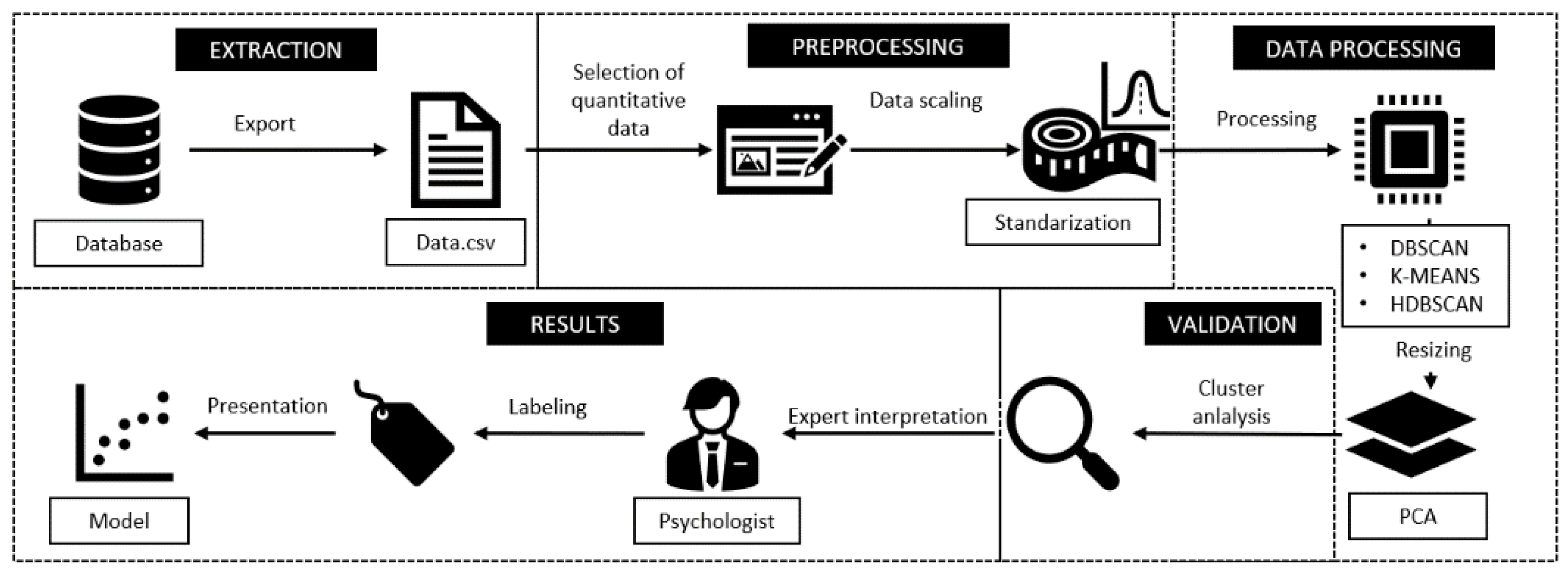
3.3. Proposed Model
3.4. Data Colection
- Study habits is a psychological questionnaire structured by 55 items. The questions evaluate the study habits and techniques used by students, which influence the learning process. The questionnaire is divided into five dimensions: how to organize to study, strategies used to solve tasks, methods used to prepare for an exam, the way you pay attention in class, and how do you study at home? The responses to the questionnaire are dichotomous (always/never). The main objective of the instrument is to categorize the academic performance of students [62,63].
- Adaptation to university life is a questionnaire focused on evaluating the academic, institutional, and social dimensions of the students, with 50 structured items. It has Likert-type assessment scale responses, from the most negative rating to the most positive rating (totally disagree/ sometimes disagree/sometimes agree/totally agree). Specifically, the questionnaire helps to determine the nature of the adaptive process of the university student [64].
- Zung’s Self-Assessment Depression Scale (SDS) is a standardized questionnaire that can be self-administered, based on norms elaborated in percentiles, with 20 structured items. It evaluates the affective, cognitive, and somatic aspects of the patients, through questions with a Likert-type assessment scale (never/sometimes/most of the time/always ). It has the aim of measuring the level of depression in a simple and specific way as a psychiatric disorder, allowing to categorize the depression level of an individual [65].
- The validated Spanish version of the Hamilton Anxiety Rating Scale (HARS) is a questionnaire and clinical assessment tool, structured in 14 items, with Likert-type responses (very disabling/severe/moderate/mild/none), which provide useful information about possible anxious-depressive symptoms to evaluate the symptomatology of an individual’s level of anxiety [66].
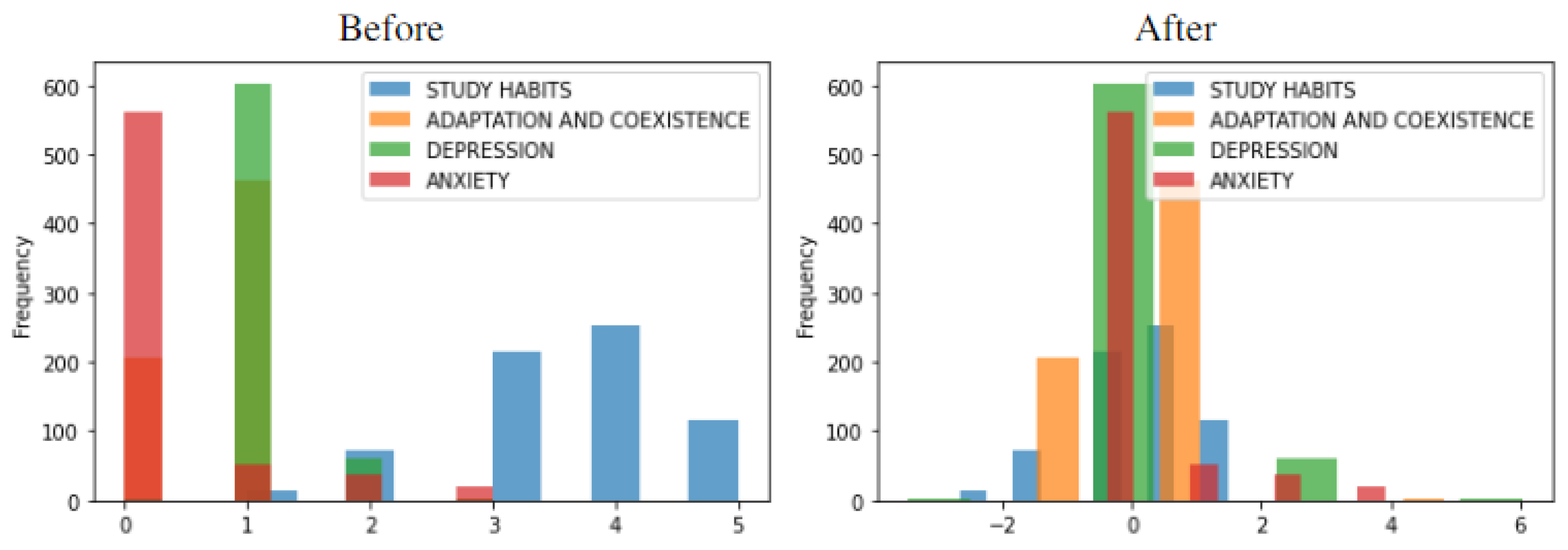
3.5. Data Pre-Processing, Processing, and Visualization
- Processing with DBSCAN
- Processing with K-Means
- Processing with HDBSCAN
4. Analysis of Results and Discussion
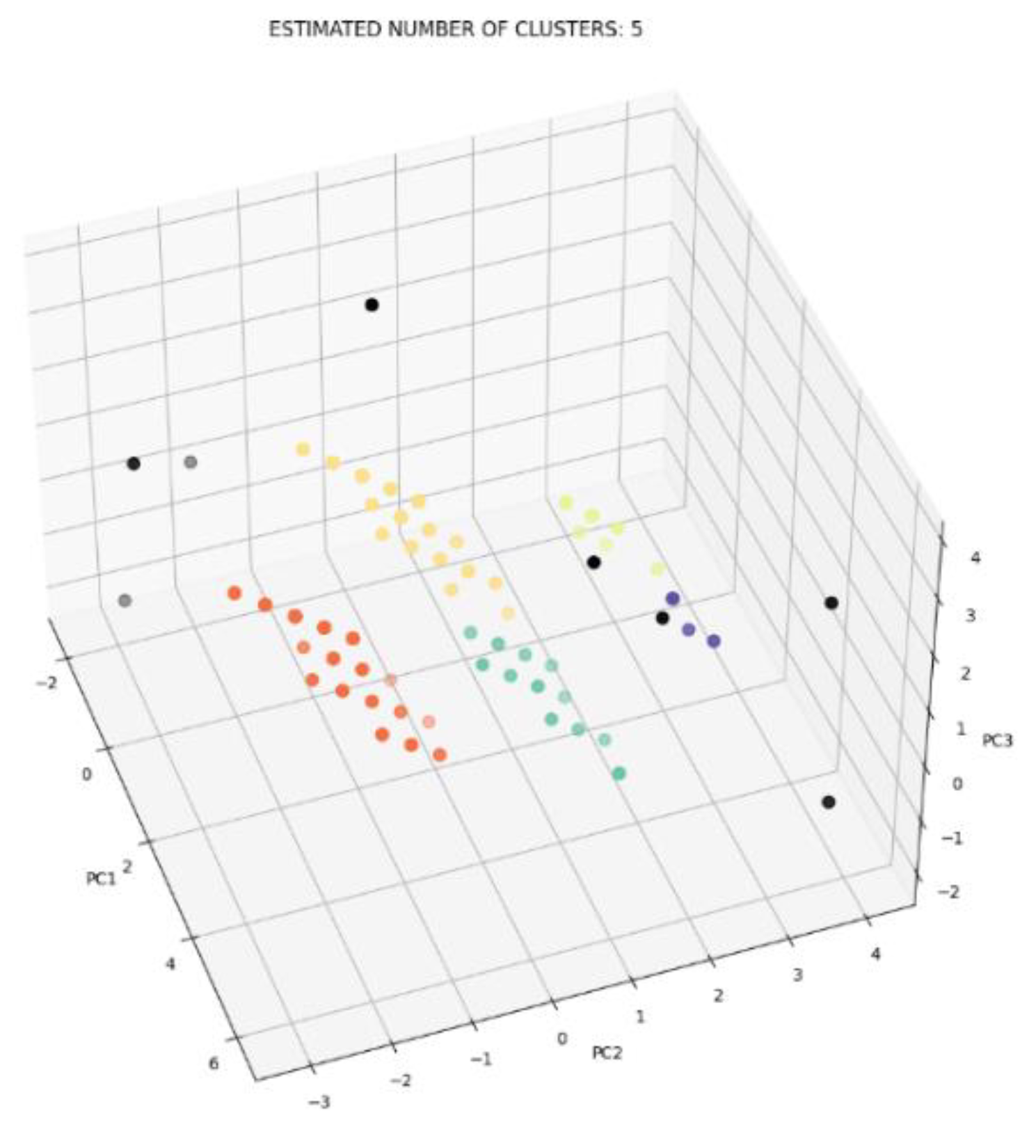
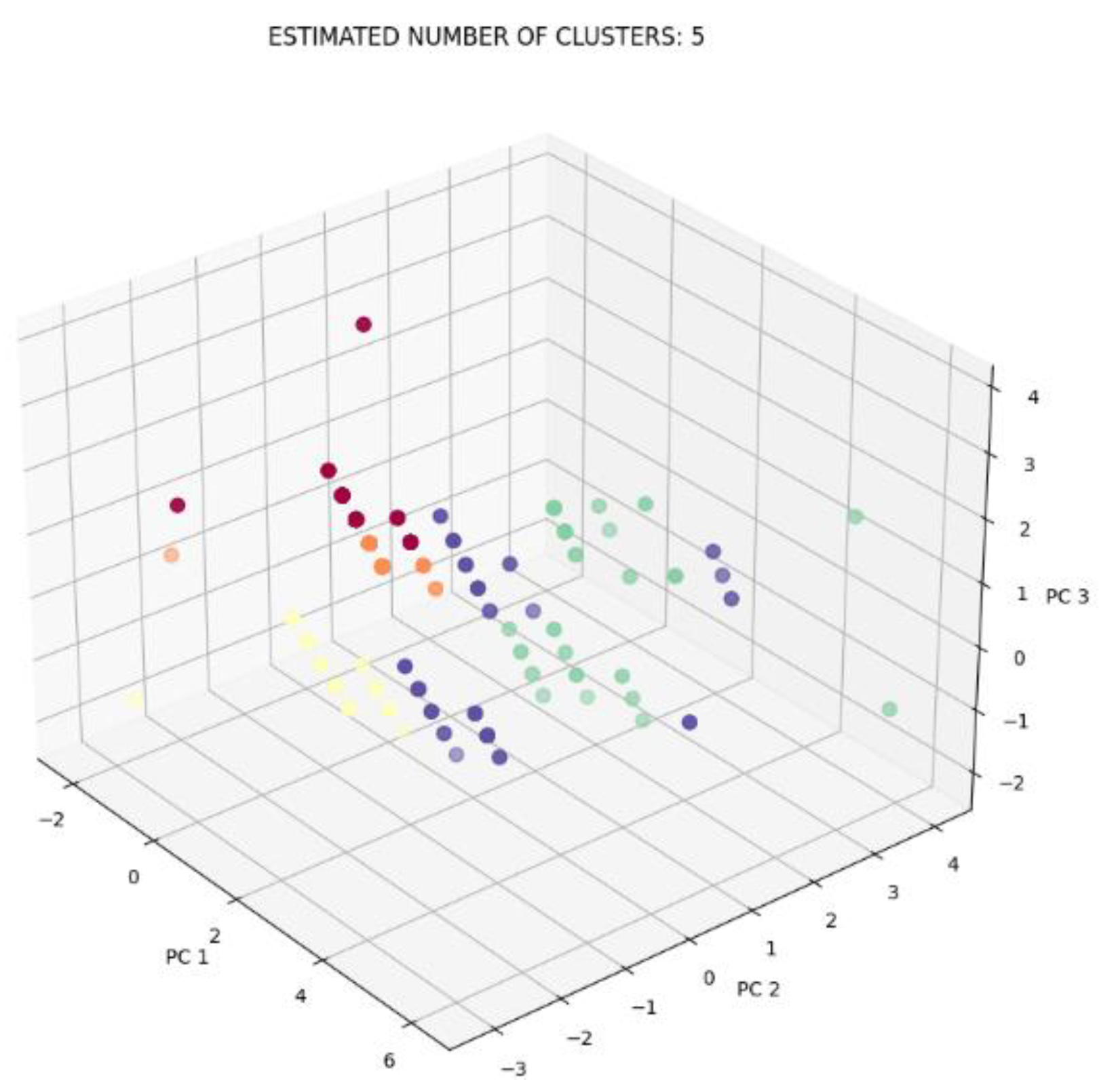
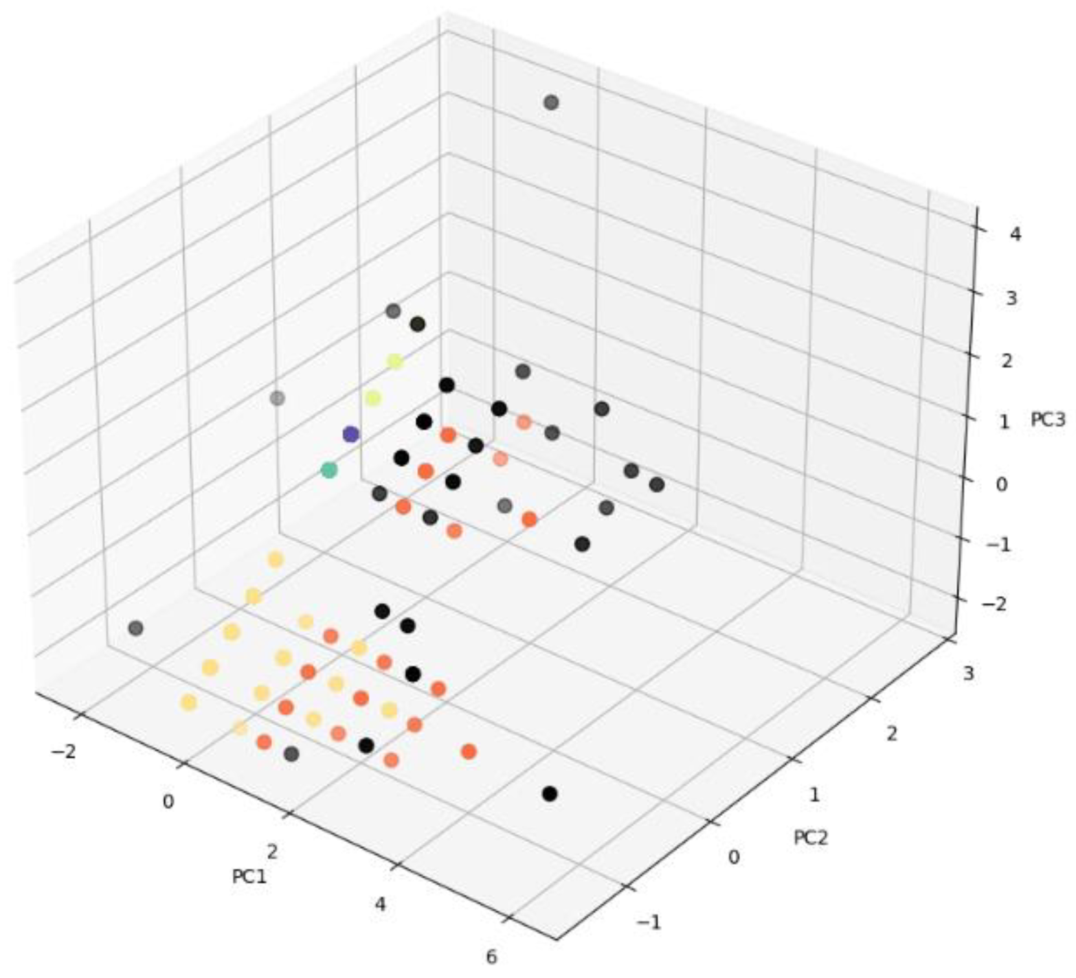
4.1. Visual Validation
4.2. Internal Validation
4.3. Expert Validacion
5. Conclusions
Author Contributions
Funding
Institutional Review Board Statement
Informed Consent Statement
Data Availability Statement
Conflicts of Interest
References
- Díaz-Méndez, M.; Paredes, M.R.; Saren, M. Improving Society by Improving Education through Service-Dominant Logic: Reframing the Role of Students in Higher Education. Sustainability 2019, 11, 5292. [Google Scholar] [CrossRef] [Green Version]
- Zarouk, M.Y.; Olivera, E.; Peres, P.; Khaldi, M. The Impact of Flipped Project-Based Learning on Self-Regulation in Higher Education. Int. J. Emerg. Technol. Learn. 2020, 15, 127–147. [Google Scholar] [CrossRef]
- Chacón-Cuberos, R.; Martínez-Martínez, A.; Puertas-Molero, P.; Viciana-Garófano, V.; González-Valero, G.; Zurita-Ortega, F. Bienestar Social En La Etapa Universitaria Según Factores Sociodemográficos En Estudiantes de Educación. Rev. Electrónica Investig. Educ. 2020, 22, e03. [Google Scholar] [CrossRef] [Green Version]
- Mejía-Navarrete, J. El Proceso de La Educación Superior En El Perú. La Descolonialidad Del Saber Universitario. Cinta de Moebio 2018, 61, 56–71. [Google Scholar] [CrossRef]
- Barreto-Osma, D.; Salazar-Blanco, H.A. Agotamiento Emocional En Estudiantes Universitarios Del Área de La Salud. Univ. y Salud 2021, 23, 30–39. [Google Scholar] [CrossRef]
- Vargas, M.; Talledo-Ulfe, L.; Heredia, P.; Quispe-Colquepisco, S.; Mejia, C.R. Influencia de Los Hábitos En La Depresión Del Estudiante de Medicina Peruano: Estudio En Siete Departamentos. Rev. Colomb. Psiquiatr. 2018, 47, 32–36. [Google Scholar] [CrossRef]
- Castillo Riquelme, V.; Cabezas Maureira, N.; Vera Navarro, C.; Toledo Puente, C. Ansiedad Al Aprendizaje En Línea: Relación Con Actitud, Género, Entorno y Salud Mental En Universitarios. Rev. Digit. Investig. Docencia Univ. 2021, 15, e1284. [Google Scholar] [CrossRef]
- Zulu, W.V.; Mutereko, S. Exploring the Causes of Student Attrition in South African TVET Colleges: A Case of One KwaZulu-Natal Technical and Vocational Education and Training College. Interchange 2020, 51, 385–407. [Google Scholar] [CrossRef]
- Aina, C.; Baici, E.; Casalone, G.; Pastore, F. The determinants of university dropout: A review of the socio-economic literature. Socio-Econ. Plan. Sci. 2021, 79, 101102. [Google Scholar] [CrossRef]
- Aguilera García, J.L. La Tutoría Universitaria Como Práctica Docente: Fundamentos y Métodos Para El Desarrollo de Planes de Acción Tutorial En La Universidad. Pro-Posições 2019, 30, e20170038. [Google Scholar] [CrossRef]
- Buring, S.M.; Williams, A.; Cavanaugh, T. The life raft to keep students afloat: Early detection, supplemental instruction, tutoring, and self-directed remediation. Curr. Pharm. Teach. Learn. 2022, 14, 1060–1067. [Google Scholar] [CrossRef] [PubMed]
- Sánchez Cabezas, P.d.P.; Luna Álvarez, H.E.; López Rodríguez del Rey, M.M. La Tutoría En La Educación Superior y Su Integración En La Actividad Pedagógica Del Docente Universitario. Conrado 2019, 15, 300–305. [Google Scholar]
- Alonso-García, S.; Rodríguez-García, A.M.; Cáceres-Reche, M.P. Analysis of the Tutorial Action and Its Impact on the Overall Development of the Students. The Case of the University of Castilla La Mancha, Spain. Form. Univ. 2018, 11, 63–72. [Google Scholar] [CrossRef]
- Mi, H.; Gao, Z.; Zhang, Q.; Zheng, Y. Research on Constructing Online Learning Performance Prediction Model Combining Feature Selection and Neural Network. Int. J. Emerg. Technol. Learn. 2022, 17, 94–111. [Google Scholar] [CrossRef]
- Guzmán-Castillo, S.; Körner, F.; Pantoja-García, J.I.; Nieto-Ramos, L.; Gómez-Charris, Y.; Castro-Sarmiento, A.; Romero-Conrado, A.R. Implementation of a Predictive Information System for University Dropout Prevention. Procedia Comput. Sci. 2022, 198, 566–571. [Google Scholar] [CrossRef]
- Chen, M.; Yan, Z.; Meng, C.; Huang, M. The Supporting Environment Evaluation Model of ICT in Chinese University Teaching. In Proceedings of the 2018 International Symposium on Educational Technology (ISET), Osaka, Japan, 31 July 2018–2 August 2018; IEEE: Piscataway, NJ, USA, 2018; pp. 99–103. [Google Scholar] [CrossRef]
- Delerna Rios, G.E.; Levano Rodriguez, D. Importancia de Las Tecnologías de Información En El Fortalecimiento de Competencias Pedagógicas En Tiempos de Pandemia. Rev. Científica Sist. Inf. 2021, 1, 69–78. [Google Scholar] [CrossRef]
- Ghareeb, S.; Hussain, A.J.; Al-Jumeily, D.; Khan, W.; Al-Jumeily, R.; Baker, T.; Al Shammaa, A.; Khalaf, M. Evaluating Student Levelling Based on Machine Learning Model’s Performance. Discov. Internet Things 2022, 2, 1–25. [Google Scholar] [CrossRef]
- Gonzalez Salas Duhne, P.; Delgadillo, J.; Lutz, W. Predicting Early Dropout in Online versus Face-to-Face Guided Self-Help: A Machine Learning Approach (Authors Masked for Peer Review). Behav. Res. Ther. 2022, 159, 104200. [Google Scholar] [CrossRef]
- Narayanasamy, S.K.; Elçi, A. An Effective Prediction Model for Online Course Dropout Rate. Int. J. Distance Educ. Technol. 2020, 18, 94–110. [Google Scholar] [CrossRef]
- Mduma, N.; Kalegele, K.; Machuve, D. A Survey of Machine Learning Approaches and Techniques for Student Dropout Prediction. Data Sci. J. 2019, 18, 1–10. [Google Scholar] [CrossRef]
- Castro-Lopez, A.; Silva Almeida, L.; Fernández Rivas, S.; Guzmán, A.; Barragán, S.; Cala-Vitery, F. Comparative Analysis of Dropout and Student Permanence in Rural Higher Education. Sustainability 2022, 14, 8871. [Google Scholar] [CrossRef]
- Guzmán, A.; Barragán, S.; Cala Vitery, F. Dropout in Rural Higher Education: A Systematic Review. Front. Educ. 2021, 6, 351. [Google Scholar] [CrossRef]
- Yi, S.; Dianatinasab, M.; Faria De Moura Villela, E.; Khanal, P.; Lin, Y.; Maluenda-Albornoz, J.; Infante-Villagrán, V.; Galve-González, C.; Flores-Oyarzo, G.; Berríos-Riquelme, J. Early and Dynamic Socio-Academic Variables Related to Dropout Intention: A Predictive Model Made during the Pandemic. Sustainability 2022, 14, 831. [Google Scholar] [CrossRef]
- Bernardo, A.B.; Galve-González, C.; Núñez, J.C.; Almeida, L.S. Settings Open AccessFeature PaperArticle A Path Model of University Dropout Predictors: The Role of Satisfaction, the Use of Self-Regulation Learning Strategies and Students’ Engagement. Sustainability 2022, 14, 1057. [Google Scholar] [CrossRef]
- Kanetaki, Z.; Stergiou, C.; Bekas, G.; Troussas, C.; Sgouropoulou, C. Analysis of Engineering Student Data in Online Higher Education During the COVID-19 Pandemic. Int. J. Eng. Pedagog. 2021, 11, 27–49. [Google Scholar] [CrossRef]
- Tayebi, A.; Gomez, J.; Delgado, C. Analysis on the Lack of Motivation and Dropout in Engineering Students in Spain. IEEE Access 2021, 9, 66253–66265. [Google Scholar] [CrossRef]
- Pavelea, A.M.; Moldovan, O. Why Some Fail and Others Succeed? Explaining the Academic Performance of PA Undergraduate Students. NISPAcee J. Public Adm. Policy 2020, 13, 109–132. [Google Scholar] [CrossRef]
- Zapata-Lamana, R.; Sanhueza-Campos, C.; Stuardo-Álvarez, M.; Ibarra-Mora, J.; Mardones-Contreras, M.; Reyes-Molina, D.; Vásquez-Gómez, J.; Lasserre-Laso, N.; Poblete-Valderrama, F.; Petermann-Rocha, F.; et al. Anxiety, Low Self-Esteem and a Low Happiness Index Are Associated with Poor School Performance in Chilean Adolescents: A Cross-Sectional Analysis. Int. J. Environ. Res. Public Health 2021, 18, 11685. [Google Scholar] [CrossRef]
- Mena, M.; Godoy, W.; Tisalema, S. Analysis of Causes of Early Dropout of Students Higher Education. Minerva 2021, 2, 79–89. [Google Scholar] [CrossRef]
- Núñez-Naranjo, A.F.; Ayala-Chauvin, M.; Riba-Sanmartí, G. Prediction of University Dropout Using Machine Learning. In Proceedings of the International Conference on Information Technology & Systems, Libertad, Ecuador, 4–6 February 2021; Springer: Cham, Switzerland, 2021; pp. 396–406. [Google Scholar] [CrossRef]
- Dalipi, F.; Imran, A.S.; Kastrati, Z. MOOC Dropout Prediction Using Machine Learning Techniques: Review and Research Challenges. In Proceedings of the 2018 IEEE Global Engineering Education Conference (EDUCON), Santa Cruz de Tenerife, Spain, 17–20 April 2018; IEEE Computer Society: Piscataway, NJ, USA, 2018; pp. 1007–1014. [Google Scholar] [CrossRef] [Green Version]
- Albreiki, B.; Zaki, N.; Alashwal, H. A Systematic Literature Review of Student’ Performance Prediction Using Machine Learning Techniques. Educ. Sci. 2021, 11, 552. [Google Scholar] [CrossRef]
- Mohamed Nafuri, A.F.; Sani, N.S.; Zainudin, N.F.A.; Rahman, A.H.A.; Aliff, M. Clustering Analysis for Classifying Student Academic Performance in Higher Education. Appl. Sci. 2022, 12, 9467. [Google Scholar] [CrossRef]
- Freitas, F.A.d.S.; Vasconcelos, F.F.X.; Peixoto, S.A.; Hassan, M.M.; Ali Akber Dewan, M.; de Albuquerque, V.H.C.; Rebouças Filho, P.P. IoT System for School Dropout Prediction Using Machine Learning Techniques Based on Socioeconomic Data. Electronics 2020, 9, 1613. [Google Scholar] [CrossRef]
- Rovira, S.; Puertas, E.; Igual, L. Data-Driven System to Predict Academic Grades and Dropout. PLoS ONE 2017, 12, e0171207. [Google Scholar] [CrossRef] [Green Version]
- Sansone, D. Beyond Early Warning Indicators: High School Dropout and Machine Learning. Oxf. Bull. Econ. Stat. 2019, 81, 456–485. [Google Scholar] [CrossRef]
- Duque Hernández, J.I.; Rodríguez-Chávez, M.H.; Polanco-Martagón, S. Caracterización Del Aprendizaje de Algoritmos Mediante Minería de Datos En El Nivel Superior. Dilemas Contemp. Educ. Política y Valores 2021, 9, 1–18. [Google Scholar] [CrossRef]
- Zuo, W.; Hou, X. An Improved Probability Propagation Algorithm for Density Peak Clustering Based on Natural Nearest Neighborhood. Array 2022, 15, 100232. [Google Scholar] [CrossRef]
- Webb, G.I.; Fürnkranz, J.; Fürnkranz, J.; Fürnkranz, J.; Hinton, G.; Sammut, C.; Sander, J.; Vlachos, M.; Teh, Y.W.; Yang, Y.; et al. Density-Based Clustering. In Encyclopedia of Machine Learning; Springer: Boston, MA, USA, 2011; pp. 270–273. [Google Scholar] [CrossRef]
- Tavakkol, B.; Choi, J.; Jeong, M.K.; Albin, S.L. Object-Based Cluster Validation with Densities. Pattern Recognit. 2022, 121, 108223. [Google Scholar] [CrossRef]
- Xie, H.; Li, P. A Density-Based Evolutionary Clustering Algorithm for Intelligent Development. Eng. Appl. Artif. Intell. 2021, 104, 104396. [Google Scholar] [CrossRef]
- Daszykowski, M.; Walczak, B. Density-Based Clustering Methods. Compr. Chemom. 2009, 2, 635–654. [Google Scholar] [CrossRef]
- Ester, M.; Kriegel, H.-P.; Sander, J.; Xu, X. A Density-Based Algorithm for Discovering Clusters in Large Spatial Databases with Noise. In Proceedings of the Second International Conference on Knowledge Discovery and Data Mining (KDD-96), Portland, OR, USA, 2–4 August 1996; AAAI Press: Washington, DC, USA, 1996; pp. 226–231. [Google Scholar]
- Li, M.; Bi, X.; Wang, L.; Han, X. A Method of Two-Stage Clustering Learning Based on Improved DBSCAN and Density Peak Algorithm. Comput. Commun. 2021, 167, 75–84. [Google Scholar] [CrossRef]
- Lloyd, S.P. Least Squares Quantization in PCM. IEEE Trans. Inf. Theory 1982, 28, 129–137. [Google Scholar] [CrossRef] [Green Version]
- Meng, Y.; Liang, J.; Cao, F.; He, Y. A New Distance with Derivative Information for Functional K-Means Clustering Algorithm. Inf. Sci. 2018, 463–464, 166–185. [Google Scholar] [CrossRef]
- Wang, F.; Wang, Q.; Nie, F.; Li, Z.; Yu, W.; Ren, F. A Linear Multivariate Binary Decision Tree Classifier Based on K-Means Splitting. Pattern Recognit. 2020, 107, 107521. [Google Scholar] [CrossRef]
- Yuan, C.; Yang, H. Research on K-Value Selection Method of K-Means Clustering Algorithm. J. Multidiscip. Sci. J. 2019, 2, 226–235. [Google Scholar] [CrossRef] [Green Version]
- Liu, F.; Deng, Y. Determine the Number of Unknown Targets in Open World Based on Elbow Method. IEEE Trans. Fuzzy Syst. 2021, 29, 986–995. [Google Scholar] [CrossRef]
- Campello, R.J.G.B.; Moulavi, D.; Sander, J. Density-Based Clustering Based on Hierarchical Density Estimates. In Lecture Notes in Computer Science (Including Subseries Lecture Notes in Artificial Intelligence and Lecture Notes in Bioinformatics); Springer: Berlin/Heidelberg, Germany, 2013; Volume 7819, pp. 160–172. [Google Scholar] [CrossRef]
- McInnes, L.; Healy, J.; Astels, S. Hdbscan: Hierarchical Density Based Clustering. J. Open Source Softw. 2017, 2, 205. [Google Scholar] [CrossRef]
- Draszawka, K.; Szymański, J. External Validation Measures for Nested Clustering of Text Documents. Stud. Comput. Intell. 2011, 369, 207–225. [Google Scholar] [CrossRef]
- Haouas, F.; Ben Dhiaf, Z.; Hammouda, A.; Solaiman, B. A New Efficient Fuzzy Cluster Validity Index: Application to Images Clustering. In Proceedings of the 2017 IEEE International Conference on Fuzzy Systems (FUZZ-IEEE), Naples, Italy, 9–12 July 2017; pp. 1–6. [Google Scholar] [CrossRef]
- Rousseeuw, P.J. Silhouettes: A Graphical Aid to the Interpretation and Validation of Cluster Analysis. J. Comput. Appl. Math. 1987, 20, 53–65. [Google Scholar] [CrossRef] [Green Version]
- Caliñski, T.; Harabasz, J. A Dendrite Method Foe Cluster Analysis. Commun. Stat. 1974, 3, 1–27. [Google Scholar] [CrossRef]
- Rendón, E.; Abundez, I.; Arizmendi, A.; Quiroz, E.M. Internal versus External Cluster Validation Indexes. Int. J. Comput. Commun. 2011, 5, 27–34. [Google Scholar]
- Davies, D.L.; Bouldin, D.W. A Cluster Separation Measure. IEEE Trans. Pattern Anal. Mach. Intell. 1979, PAMI-1, 224–227. [Google Scholar] [CrossRef]
- Zhang, E.; Zhang, Y. F-Measure. In Encyclopedia of Database Systems; Springer: New York, NY, USA, 2018; pp. 1492–1493. [Google Scholar] [CrossRef]
- Bagunaid, W.; Chilamkurti, N.; Veeraraghavan, P. AISAR: Artificial Intelligence-Based Student Assessment and Recommendation System for E-Learning in Big Data. Sustainability 2022, 14, 10551. [Google Scholar] [CrossRef]
- Rovetta, S.; Masulli, F.; Cabri, A. The “Probabilistic Rand Index”: A Look from Some Different Perspectives. In Smart Innovation, Systems and Technologies; Springer Science and Business Media Deutschland GmbH: Singapore, 2020; Volume 151, pp. 95–105. [Google Scholar] [CrossRef]
- Benitez Molina, A.; Caballero Badillo, M.C. Psychometric Study of the Depression, Anxiety and Family Dysfunction Scales in Students at Universidad Industrial de Santander. Acta Colomb. Psicol. 2017, 20, 221–231. [Google Scholar] [CrossRef] [Green Version]
- De la Parra Paz, E. Herencia de Vida Para Tus Hijos: Crecimiento Integral Con Técnicas PNL; Grijalbo Mondadori: Barcelona, Spain, 2004. [Google Scholar]
- Almeida, L.S.; Soares, A.P.C.; Ferreira, J.A. Questionário de Vivências Acadêmicas (QVA-r): Avaliação Do Ajustamento Dos Estudantes Universitários. Avaliação Psicológica 2002, 1, 81–93. [Google Scholar]
- Hamilton, M. The Assessment of Anxiety States by Rating. Br. J. Med. Psychol. 1959, 32, 50–55. [Google Scholar] [CrossRef] [PubMed]
- Lobo, A.; Chamorro, L.; Luque, A.; Dal-Ré, R.; Badia, X.; Baró, E. Validación de Las Versiones En Español de La Montgomery-Asberg Depression Rating Scale y La Hamilton Anxiety Rating Scale Para La Evaluación de La Depresión y de La Ansiedad. Med. Clin. (Barc.) 2002, 118, 493–499. [Google Scholar] [CrossRef]
- Evangelista, E.D. A Hybrid Machine Learning Framework for Predicting Students’ Performance in Virtual Learning Environment. Int. J. Emerg. Technol. Learn. 2021, 16, 255–272. [Google Scholar] [CrossRef]


| Column | Type |
|---|---|
| code | string |
| study habits | int |
| adaptation and coexistence | int |
| depression | int |
| anxiety | int |
| Index | Study Habits | Adaptation and Coexistence | Depression | Anxiety |
|---|---|---|---|---|
| count | 670 | 670 | 670 | 670 |
| mean | 3.5731 | 0.6985 | 1.0940 | 0.2746 |
| SD | 0.9673 | 0.4784 | 0.3166 | 0.6975 |
| min | 1 | 0 | 0 | 0 |
| 25% | 3 | 0 | 1 | 0 |
| 50% | 4 | 1 | 1 | 0 |
| 75% | 4 | 1 | 1 | 0 |
| max | 5 | 3 | 3 | 3 |
| Column | Type | Labels |
|---|---|---|
| study habits | 0–5 | (very negative, negative, negative trend, positive trend, positive, very positive) |
| adaptation and coexistence | 0–2 | (low, medium, high) |
| depression | 0–3 | (normal, light, moderate, severe) |
| anxiety | 0–3 | (mild, moderate, serious, severe) |
| Index | Number of Clusters | Silhouette | Calinski–Harabasz | Davies–Bouldin | Eps | MinPts | Noise |
|---|---|---|---|---|---|---|---|
| 25 | 5 | 0.4972 | 190.7099 | 0.9571 | 1.7 | 6 | 9 |
| 35 | 4 | 0.4919 | 220.9307 | 1.1153 | 1.8 | 12 | 13 |
| 43 | 4 | 0.4919 | 220.9307 | 1.1153 | 1.9 | 12 | 13 |
| 51 | 4 | 0.4919 | 220.9307 | 1.1153 | 2 | 12 | 13 |
| Index | Number of Clusters | Silhouette | Calinski–Harabasz | Davies–Bouldin | Minimum Cluster Size | Minimum Samples | Noise |
|---|---|---|---|---|---|---|---|
| 8 | 5 | 0.6823 | 369.6459 | 0.6563 | 55 | 19 | 63 |
| 7 | 5 | 0.6704 | 349.5316 | 0.6677 | 55 | 18 | 59 |
| 2 | 5 | 0.6639 | 334.9714 | 0.6861 | 60 | 17 | 56 |
| 6 | 5 | 0.6639 | 334.9714 | 0.6861 | 60 | 17 | 56 |
| Algorithm | Silhouette | Calinski–Harabasz | Davies–Bouldin | Number of Clusters | Noise |
|---|---|---|---|---|---|
| DBSCAN | 0.4972 | 190.7099 | 0.9571 | 5 | 9 |
| K-Means | 0.5586 | 406.4509 | 0.8001 | 5 | - |
| HDBSCAN | 0.6823 | 369.6459 | 0.6563 | 5 | 63 |
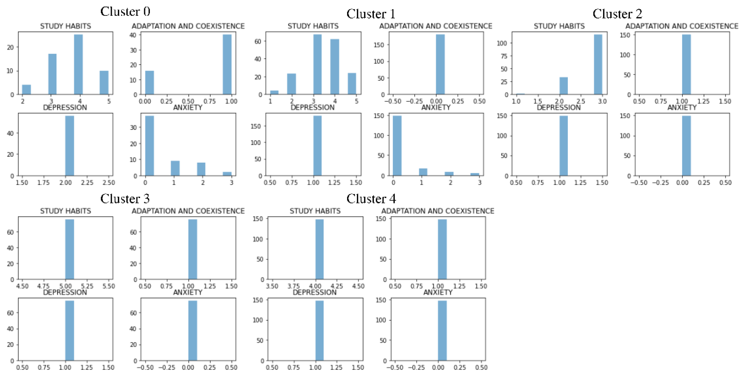
| Cluster | Study Habits | Adaptation and Coexistence | Depression | Anxiety | Risk Level |
|---|---|---|---|---|---|
| Cluster 0 | 3.7321 | 0.71429 | 2 | 0.5536 | 5 = Very high |
| Cluster 1 | 3.4389 | 0 | 1 | 0.2944 | 4 = High |
| Cluster 2 | 2.7651 | 1 | 1 | 0 | 3 = Middle |
| Cluster 3 | 5 | 1 | 1 | 0 | 1 = Very low |
| Cluster 4 | 4 | 1 | 1 | 0 | 2 = Low |
| Index | Score |
|---|---|
| F-measure | 0.909 |
| Purity | 0.945 |
| V-measure | 0.869 |
| Adjusted Rand Index | 0.865 |
Publisher’s Note: MDPI stays neutral with regard to jurisdictional claims in published maps and institutional affiliations. |
© 2022 by the authors. Licensee MDPI, Basel, Switzerland. This article is an open access article distributed under the terms and conditions of the Creative Commons Attribution (CC BY) license (https://creativecommons.org/licenses/by/4.0/).
Share and Cite
Valles-Coral, M.A.; Salazar-Ramírez, L.; Injante, R.; Hernandez-Torres, E.A.; Juárez-Díaz, J.; Navarro-Cabrera, J.R.; Pinedo, L.; Vidaurre-Rojas, P. Density-Based Unsupervised Learning Algorithm to Categorize College Students into Dropout Risk Levels. Data 2022, 7, 165. https://doi.org/10.3390/data7110165
Valles-Coral MA, Salazar-Ramírez L, Injante R, Hernandez-Torres EA, Juárez-Díaz J, Navarro-Cabrera JR, Pinedo L, Vidaurre-Rojas P. Density-Based Unsupervised Learning Algorithm to Categorize College Students into Dropout Risk Levels. Data. 2022; 7(11):165. https://doi.org/10.3390/data7110165
Chicago/Turabian StyleValles-Coral, Miguel Angel, Luis Salazar-Ramírez, Richard Injante, Edwin Augusto Hernandez-Torres, Juan Juárez-Díaz, Jorge Raul Navarro-Cabrera, Lloy Pinedo, and Pierre Vidaurre-Rojas. 2022. "Density-Based Unsupervised Learning Algorithm to Categorize College Students into Dropout Risk Levels" Data 7, no. 11: 165. https://doi.org/10.3390/data7110165