Supporting Decision-Making Process on Higher Education Dropout by Analyzing Academic, Socioeconomic, and Equity Factors through Machine Learning and Survival Analysis Methods in the Latin American Context

Abstract

The prediction of university dropout is a complex problem, given the number and diversity of variables involved. Therefore, different strategies are applied to understand this educational phenomenon, although the most outstanding derive from the joint application of statistical approaches and computational techniques based on machine learning. Student Dropout Prediction (SDP) is a challenging problem that can be addressed following various strategies. On the one hand, machine learning approaches formulate it as a classification task whose objective is to compute the probability of belonging to a class based on a specific feature vector that will help us to predict who will drop out. Alternatively, survival analysis techniques are applied in a time-varying context to predict when abandonment will occur. This work considered analytical mechanisms for supporting the decision-making process on higher education dropout. We evaluated different computational methods from both approaches for predicting who and when the dropout occurs and sought those with the most-consistent results. Moreover, our research employed a longitudinal dataset including demographic, socioeconomic, and academic information from six academic departments of a Latin American university over thirteen years. Finally, this study carried out an in-depth analysis, discusses how such variables influence estimating the level of risk of dropping out, and questions whether it occurs at the same magnitude or not according to the academic department, gender, socioeconomic group, and other variables.

1. Introduction

Student dropout is one of the most-complex and -adverse events for students and institutions. Possible reasons that lead a student to abandon his/her studies are diverse and may be due to academic, demographic, or socioeconomic factors related to the familiar, affective, or university environment [1]. Addressing this problem is challenging for any educational institution since we seek to prevent it while maintaining high academic standards in student training. Some first attempts to solve this educational phenomenon employed theoretical models by creating and managing student support services, as formulated by Tinto [2]. Tinto’s model mirrors the iterative process an undergraduate student experiences throughout the academic years, pondering a possible decision between dropout or persevering. Although quite simple, several educational institutions use Tinto’s model as a reference [3]. The evolution of machine learning techniques has been essential and decisive in addressing different educational phenomena such as the impact of curricular changes [4], academic performance [5], retention [6], and dropout [5,6,7].

Predicting the early dropout of students using data is a relevant problem in education analyzed in different forms and teaching–learning environments. Initially, the SDP problem employed classification algorithms, which were successfully implemented in [8,9,10]. However, this problem is enough to predict the abandonment or not of students but requires a deeper analysis to estimate the permanence time. Generally, a student is likelier to drop out during the first years since there is a direct relationship between the permanence time at university and the probability of dropping out, as mentioned by Aulck et al. [11].

Survival analysis methods emerge as an alternative to formulate the SDP problem more comprehensively and profoundly. These methods not only predict the occurrence of the student dropping out or not, but it is also possible to estimate the probability that the dropout would occur at a certain time [12]. With the rise of machine learning, new variants of survival models have been developed and applied in various areas, mainly in biomedical areas [13,14]. The Cox Proportional Hazards regression model (CPH) is the best-known and most-applied model in multiple contexts. Ameri et al. [12] developed a survival analysis framework for early attrition prediction using CPH and variants such as Time-Dependent regression Cox (TDCox). In addition, a variation to CPH based on deep neural networks was introduced by Katzman et al. [15]. The literature also includes variants of survival analysis derived from machine learning, such as Multitask logistic regression [16,17], and Random survival forests [18,19]. Pan et al. [20] explored various survival analysis techniques and compared them with their proposal. They introduced a deep learning model assuming dispersion and volatility, which they named SAVSNet. Furthermore, transformer variants for survival analysis were implemented by [21,22]. For example, S. Hu [22] validated these variants with data from cancer patients.

Although many works address the computational techniques of machine learning and survival analysis, just a few compare these models jointly. Gutierrez Pachas et al. [23] presented a methodology to determine who would drop out and when the drop would be in a real dataset from 655 students of one program at a Peruvian university and evaluated the influence of predictor variables using statistical inference tools. Garcia-Zanabria et al. [24] developed a visual and interactive tool that allowed construction situations from counterfactuals and prevented the dropout of students at risk.

Our work evaluated multiple machine learning algorithms and survival analysis methods and their deep variants on a dataset of students from six academic departments of a Latin American university. We documented the appropriate treatment of the predictor variables to apply both approaches together. Our analysis aimed to use these techniques as computational support to help academic managers efficiently identify those students at risk and interpret the impact of academic, socioeconomic, and equity variables in the Latin American context. In addition, we present an in-depth review of diverse techniques for the SDP problem. Finally, we performed a deep analysis of academic variables’ influence when estimating the level of risk of dropping out and questioned whether it occurs in the same magnitude or not.

2. Formulation of the SDP Problem

Given a dataset of N observations, we introduce basic notations to formulate the SDP problem. For each student i, $\forall i=1,\dots ,N$,

• ${\overrightarrow{X}}_i$ is the n-dimensional vector of attributes.
• $Y_i$ is the output variable.
• $E_i$ is the event variable such that $E_i=1$, if the dropout happens, otherwise $E_i=0$.
• $T_i$ is the time variable, i.e., $T_i$ represents the permanence time at the university.

First, we define the SDP problem as a classification task and then as a survival analysis model. The main difference between these approaches is representing the output variable $Y_i$. Furthermore, we denote ${\widehat{Y}}_i$ to represent the estimated value of $Y_i$. Similar notations are used for ${\widehat{E}}_i$ and ${\widehat{T}}_i$.

2.1. SDP Problem as a Classification Model

The goal is to predict whether a student will drop out or not, given a fixed set of features. The probability that the student drops out is:

$$p_i^{\mathrm{c}}\left(X\right)=\mathrm{Prob}(E_i=1|X={\overrightarrow{X}}_i).$$

(1)

Generally, if $p_i^{\mathrm{c}}\left(X\right)>0.5$, then he/she is a dropout student, otherwise she/he is not. However, the computation of $p_i^{\mathrm{c}}$ is time-invariant. For this reason, we must be careful when choosing the predictor variables to avoid calculating $p_i^{\mathrm{c}}$ in a biased mode. Therefore, according to this approach, we write $Y_i=E_i$.

2.2. SDP Problem as a Survival Analysis Model

Survival analysis models seek to estimate the time until they precede to abandonment. We define the probability that the student drops out at the time t, given his/her permanence before t, as follows:

$$p_i^{\mathrm{s}}(X,t)=\mathrm{Prob}(T_i=t|T_i>t-1,X={\overrightarrow{X}}_i).$$

(2)

Therefore, the survival probability $S_i(X,t)$ is defined by

$$S_i(X,t)=\prod _{\tau =0}^t\left(1-p_i^{\mathrm{s}}(X,\tau )\right).$$

(3)

In general, the survival probability is a monotone non-increasing function. Nevertheless, we denominate censored information when the student’s dropout (that is, $E_i=0$) does not occur during the time interval under analysis. Survival time has two components that must be clearly defined: a beginning point and an endpoint that is reached either when the event occurs or when the follow-up time has ended. One fundamental concept needed to understand survival analysis is censoring:

(a)

The dropout occurred, and we can measure when it occurred ($T_i$).

(b)

The dropout did not occur when we observed the student; we only know the number of semesters in which it did not occur ($C_i$), named censoring time.

Also, we define $Y_i=\min (T_i,C_i)$. In Figure 1a, we visualize the permanence times of four students. We notice that student B dropped out in the first semester, while Student D dropped out of the university in the fourth semester. Furthermore, A and C correspond to censored data. Figure 1b shows the survival curves for the students A, B, C, and D. Student B has a very low probability of remaining in his/her studies after the second semester. The opposite occurs with C, who has a high survival probability each time.

3. Related Work

This section presents a profound and detailed review of the related works that handle the SDP problem according to the computational techniques employed.

3.1. Machine Learning Algorithms

Our literature review included the evaluation of various algorithms, such as Logistic Regression (LR) [25,26], Gaussian Naive Bayes (GNB) [25], Support Vector Machine (SVM) [26], Decision Trees (DTs) [25,26], K-Nearest Neighbors (KNNs) [27], Random Forest (RF) [28], Bayesian Networks (BNs) [28], Artificial Neural Networks (ANNs) [29,30], and Convolutional Neural Networks (CNNs) [31,32,33]. Vásquez Verdugo and Miranda [26] investigated a dataset of students in a business program at a Chilean university and obtained that SVM had the best predictive capacity in most cases; it was only inferior to LR when evaluating fifth- and sixth-semester students.

Medina et al. [28] compared BNs with DTs from a dataset of 500 students from a private university in Lima. They concluded that the BN was the best model when comparing the precision, accuracy, and specificity metrics. In contrast, Mezzini et al. [31] analyzed 6000 students from the Education Department of Rome Tre University, implemented multiple CNN variants, and obtained an accuracy value of 67.1% for first-year and 90.9% for second-year students. Furthermore, they mentioned that with more data, it is possible to develop more accurate predictions. Also, Garcia-Zanabria et al. [24] presented a visual tool that supports educational decisions based on counterfactual techniques.

The investigations described above illustrate case studies associated with face-to-face education, as well as in the online format [8,9,10]. For example, Prenkaj et al. [9] presented an extensive review of the various computational techniques and the SDP problem’s modeling, including machine learning algorithms and deep variants. Also, they classified the computational techniques according to the following aspects: field of study, gathered data, student modeling, methods, and evaluation.

3.2. Survival Analysis Methods

The tools of survival analysis have been successfully applied in various real-world domains such as health science [14], credit risk [34], and multiple applications that require estimating the time until an event of interest occurs. Wang et al. [13] presented an extensive review and detailed non-parametric methods that are traditionally used to analyze how a population sample behaves, such as the Kaplan–Meier (KM) and Nelson–Aelen (NA) estimators. These methods do not use attributes to estimate a student’s survival curve. However, they can be used to perform a full/sampled statistical analysis [4,35,36]. In contrast, parametric survival analysis models employ theoretical probability distributions. Among the best known, we have the exponential, Weibull, and Gompertz distributions.

As a hybrid of the parametric and non-parametric approaches, semi-parametric models can obtain a more robust estimator under a broader range of conditions. The Cox Proportional Hazards model (CPH) is one of the most-used survival analysis methods. Cox [37] made the assumption that covariates are independent of time. However, Time-Dependent Cox regression (TD-Cox) captures time-varying factors and can leverage that information to provide a more accurate prediction. To address the SDP problem, several works employed CPH as part of their formulation [4,6,12,15,20,23,35,38]. Gutierrez-Pachas et al. [4] used the KM estimator and CPH to analyze the impact of curricular design in a computer science program. In contrast, Ameri et al. [12] used CPH and TD-Cox to detect early student dropout. In contrast, survival analysis models based on machine learning, such as Multi-Task Logistic Regression (MTLR) [16], Random Survival Forest (RSF) [18], and Conditional Survival Forest (CSF) [19], are little used. Some applications of these techniques for the SDP problem were reported by [14,15].

3.3. Deep Learning Methods

Deep learning methods generally exploit a large volume of data to generate accurate models in diverse contexts. Agrusti et al. [39] employed real data of about 6000 students to train a CNN and predict whether the student would drop out. Mubarak et al. [33] proposed a hyper-model of Convolutional Neural Networks and Long Short-Term Memory (CONV-LSTM) to extract features from MOOCs’ raw data and predict whether each student will drop out or complete his/her courses.

In the context of survival analysis, deep learning variations have been introduced and tested in biomedical areas such as Nonlinear Cox regression (DeepSurv) [15] and Neural Multi-Task Logistic Regression (N-MTLR) [17]. For instance, Fotso [17] demonstrated that N-MTLR consistently outperforms MTLR and yields similar or better results than CPH when evaluating the concordance index in the Worcester Heart Attack Study dataset.

Recently, Pan et al. [20] introduced a Survival-Analysis-based Volatility and Sparsity modeling Network (SAVSNet) into an end-to-end deep learning framework. The SAVSNet smooths the volatile time series by a convolutional network while preserving the original data information using a long short-term memory network. They compared the SAVSNet with other survival analysis methods using the KDDCup 2015 and XuetangX datasets. Lee et al. [21] proposed DeepHit, which uses a deep neural network to learn the distribution of survival times directly. In contrast, S. Hu [22] proposed a transformer-based survival analysis method that estimates the patient-specific survival distribution. In [22] used an ordinal regression to optimize the survival probabilities over time and penalize randomized discordant pairs.

Finally, we summarize the computational techniques mentioned in Section 3.1, Section 3.2 and Section 3.3 and group them in

Table 1. Summary of references focused on the SDP problem and grouped according to classification algorithms and survival analysis methods. Additionally, we detail if the method uses a traditional approach (Trad) or a deep learning variant (Deep) in the column Type.

Family	Type	Method	Reference
		Logistic Regression (LR)	[11,23,25,26]
		K-Nearest Neighbor (KNN)	[11,27]
		Support Vector Machine (SVM)	[11,23,26]
Classification	Trad	Gaussian Naive Bayes (GNB)	[23,25,36]
Algorithms		Decision Tree (DT)	[23,25,26,28]
		Random Forest (RF)	[11,23]
		Artificial Neural Networks (ANNs)	[26,29,39]
	Deep	Convolutional Neural Networks (CNNs)	[8,9,10,32,33]
		Non-parametric methods (KM estimator)	[23,35,36]
		Parametric methods (Gompertz distribution)	[20]
Survival	Trad	Cox Proportional Hazards regression (CPH)	[4,6,12,15,20,23,35,38]
Analysis		Time-Dependent Cox regression (TD-Cox)	[12]
Methods		Random Survival Forest (RSF)	[14,15]
		Conditional Survival Forest (CSF)	[14,20]
	Deep	Nonlinear Cox regression (DeepSurv)	[15,20]

according to the classification algorithms and survival analysis methods. Mainly, our objective was to present both approaches and, in this manner, make better predictions of the dropout occurring and the time at which it would happen. Furthermore, our work addressed the techniques detailed in Table 1 employing a real dataset from six departments of a Latin American university.

4. Research Questions

To better understand our work, we present the research questions that help in applying these techniques and support understanding various problems that educational managers cannot identify:

• RQ1: How do we understand the impact of academic, socioeconomic, and equity variables on the SDP problem?
• RQ2: What is the most-efficient classification algorithm for the SDP problem?
• RQ3: What is the most-efficient survival analysis method for the SDP problem?
• RQ4: How influential is academic performance in estimating dropout risk?

5. Materials and Methods

This section describes the materials and methods used in this research. Initially, we detail the population and the sample used, as well as the pre-processing of the variables involved. Next, we perform a detailed exploratory analysis for each academic program. Finally, we introduce the main metrics to evaluate the classification algorithms and survival analysis methods.

5.1. Population and Sample

Our study population corresponds to the student demographic, socioeconomic, and academic information of a Latin American university. The time horizon of these data is thirteen years, including the first semesters of 2008 (2008-01) to the second semester of 2020 (2020-02). We obtained these data with the collaboration of the IT department, which was responsible for masking this sensitive data. Thus, we did not have access to the student’s name nor personal information, preserving the student’s identity. The personal masked Identity (ID) is unique; however, the ID is different from the masked Student Identity (SID), which is not necessarily unique for each person. A person has a unique ID, but can have one or more SIDs. This situation occurs when a student withdraws from the university and rejoins. However, in practice, we limited our dataset to one SID by the ID; this means that we only used one observation for each person, but stored whether she/he was previously enrolled in any program at this university.

In this paper, we used a sample of 13,696 students from six different departments: Education (Edu), Computer Science (CS), Psychology (Psy), Law and Political Sciences (LPS), Economic and Business Sciences (EBS), and Engineering (Eng). The sample for each department was balanced according to the dropout status. In other words, half of the students were dropouts, and the others were not.

Table 2. Distribution of the sample by academic department.

Department	Sample Size
Education (Edu)	312
Computer Science (CS)	768
Psychology (Psy)	1146
Law and Political Sciences (LPS)	2456
Economic and Business Sciences (EBS)	4100
Engineering (Eng)	4914

summarizes the distribution of the sample according to the duration of the programs and the sample size.

5.2. Data Preprocessing

Firstly, we created a new variable labeled Change_SID, which identifies whether or not the person changed his/herSID. Similarly, some demographic attributes were altered to define categorical variables, such as Female, Married, Public_School, and Scholarship. Numerical variables were defined, such as the student’s age when she/he was admitted to the university (Age_Admission). Linking students’ locations of provenance and residence with the value of the 2019 Human Development Index (HDI), we define socioeconomic variables labeled HDI_Provenance and HDI_Residence, respectively. Our dataset has the name of the admission semester, which can be regular or not. For example, 2001-01 and 2001-02 are regular semesters, and other configurations are non-regular semesters. They are resources that satisfy the number of hours and credits as summer courses.

Related to the academic variables, all grades per course were weighted to obtain the final grade point average (Final_GPA). We used the number of semesters enrolled, the number of hours of absences, the number of approved courses, and the total number of courses to determine proportional variables between them. For example, Courses_Sem represents the proportion of enrolled courses concerning the number of enrolled semesters, computed by

$$\mathtt{Courses}\_\mathtt{Sem}=\frac{\mathrm{Total}\mathrm{number}\mathrm{of}\mathrm{enrolled}\mathrm{courses}}{\mathrm{Total}\mathrm{number}\mathrm{of}\mathrm{enrolled}\mathrm{semesters}}.$$

Analogously, we calculated Absences_Courses, Approved_Courses, and NonReg_Courses. We processed the student status and assumed that students drop out when their student status is separated, retired, or transferred. Otherwise, the student did not drop out, and consequently, we defined an event variable labeled Dropout. Finally, we employed the number of completed semesters as the time variable, labeled Completed_Sem. The data cleaning and filtering were performed using Pandas and Numpy. All attributes employed in this work are summarized in

Table 3. Description of the attributes collected.

Attribute Name	Attribute Description	Attribute Type
SID	Masked student identifier	Numerical and anonymized
Department	Academic department’s name	Categorical (Edu or CS or Psy or LPS or EBS or Eng)
Changed_SID	Whether the student changed SID	Categorical (Yes or No)
Female	Whether the student’s gender is female	Categorical (Yes or No)
Married	Whether the student’s marital status is married	Categorical (Yes or No)
Public	Whether the type of student’s high school is public	Categorical (Yes or No)
Scholarship	Whether the student had a scholarship	Categorical (Yes or No)
Age_Admission	Student’s age when admitted by the university	Discrete numerical
HDI_Provenance	Human development index of the student’s location of provenance	Continuous numerical
HDI_Residence	Human development index of the student’s location of residence	Continuous numerical
Final_GPA	Final grade point average	Continuous numerical
Courses_Sem	Proportion of enrolled courses in relation to the number of enrolled semesters	Continuous numerical
Absences_Courses	Proportion of the number of hours of absence in relation to the total number of hours in courses	Continuous numerical
Approved_Courses	Proportion of approved courses in relation to the total number of enrolled courses	Continuous numerical
NonReg_Courses	Proportion of non-regular courses in relation to the total number of enrolled courses	Continuous numerical
Completed_Sem	Number of completed semesters	Discrete numerical
Dropout	Dropout status	Categorical (Yes or No)

.

5.3. Data Exploration

This section presents a detailed statistical and descriptive analysis of the attributes selected from Table 3. First, we computed the percentage distribution of the categorical variables and organized them in

Table 4. Percentage distribution of categorical attributes. We highlight the best (in green) and worst (in brown) percentage with the categorical value “Yes”.

Categorical	Edu		CS		Psy		LPS		EBS		Eng
Attribute	Yes	No	Yes	No	Yes	No	Yes	No	Yes	No	Yes	No
Changed_SID	11.9%	88.1%	23.7%	76.3%	14.2%	85.8%	19.6%	80.4%	23.0%	77.0%	24.3%	75.7%
Female	91.7%	8.30%	16.8%	83.2%	76.2%	23.8%	61.0%	39.0%	55.4%	44.6%	44.6%	55.4%
Married	1.60%	98.4%	0.40%	99.6%	1.80%	98.2%	0.90%	99.1%	0.90%	99.1%	0.30%	99.7%
Public	30.1%	69.9%	23.1%	76.9%	18.7%	81.3%	22.6%	77.4%	19.8%	80.2%	23.2%	76.8%
Scholarship	12.2%	87.8%	4.70%	95.3%	3.90%	96.1%	4.00%	96.0%	1.80%	98.2%	5.80%	94.2%

. We colored the cells green and brown to highlight the best and worst percentages, respectively. Analyzing Table 4, we find essential insights that help us better understand our dataset. In Edu, 91.7% of the students are women, in contrast to CS, where 16.8% are female students. Furthermore, Edu has the highest percentage of students from public high schools (Public) and even stands out for having the highest rate of students according to the variable Scholarship. This is because, usually, in Latin America, low-income people study in public schools.

The percentage of married students (Married) is low in all departments. We notice the highest value in Psy with 1.8%. Furthermore, the highest values of Changed_SID occur in Eng, and the opposite happens in Edu.

In the context of the numerical attributes, we computed the mean and the standard deviation (Std) and summarize them in

Table 5. Mean and standard deviation (std) of numerical attributes. We highlight the best (in green) and worst (in brown) mean values.

Numerical	Edu		CS		Psy		LPS		EBS		Eng
Attribute	mean	std	mean	std	mean	std	mean	std	mean	std	mean	std
Age_Admission	20.68	3.19	19.21	2.87	19.35	3.43	18.52	2.53	18.91	2.72	18.39	2.08
HDI_Provenance	0.71	0.10	0.71	0.09	0.71	0.09	0.71	0.10	0.71	0.10	0.70	0.10
HDI_Residence	0.66	0.12	0.66	0.11	0.67	0.11	0.66	0.11	0.67	0.11	0.66	0.11
Final_GPA	12.67	3.12	11.12	3.36	11.94	3.34	11.99	2.93	11.72	2.85	11.22	2.85
Courses_Sem	6.83	3.02	5.58	2.48	6.63	3.12	6.49	2.94	6.07	0.11	5.67	2.4
Absences_Courses	0.14	0.11	0.13	0.12	0.12	0.11	0.14	0.10	0.14	0.10	0.12	0.11
Approved_Courses	0.72	0.27	0.62	0.28	0.65	0.31	0.66	0.28	0.65	0.27	0.61	0.27
NonReg_Courses	0.04	0.06	0.06	0.08	0.06	0.06	0.06	0.06	0.06	0.06	0.08	0.06

. We noticed that the data distribution according to HDI_Provenance, HDI_Residence and Absences_Courses is similar for each academic department. However, in Edu, we found that the mean of Final_GPA is higher than the mean value of the other departments. In contrast, this does not happen in STEM areas such as CS and Eng, making us think that STEM careers tend to be more complicated. A similar context occurs with other academic variables, such as Approved_Courses and Courses_Sem.

5.4. Computational Techniques and Evaluation Metrics

The initial step in executing these techniques is randomly dividing the dataset: 70% was used for training and the rest for testing. Cross-validation is a technique in which models are trained using subsets of the dataset and then evaluated using the complementary subsets. Three main steps are involved in cross-validation, which are:

• Reserving a subset of the data.
• Using the rest of the dataset to train the model.
• Testing the model using the reserved subset of data.

Cross-validation techniques have many methods; the most commonly used is k-fold cross-validation. In k-fold cross-validation, the dataset is split into k subsets (folds). Training is then performed on all subsets, except one (reserved subset), which is then used to test the model. The method is iterated k times with different reserved subsets for each iteration.

The first approach consists of defining the SDP problem as a classification task and measuring it utilizing metrics such as precision, recall, and accuracy. Generally, these values are obtained from a binary confusion matrix. For example, accuracy is:

$$\mathrm{Accuracy}=\frac{\mathrm{TP}+\mathrm{TN}}{\mathrm{TP}+\mathrm{FP}+\mathrm{TN}+\mathrm{FN}},$$

(4)

where TP and TN represent the number of true positive and true negative cases. We use similar notation for FP and FN. The Receiver Operating Characteristic curve (ROC) is a graph showing the performance of a classification model at all classification thresholds. This curve plots two parameters, the True Positive Rate (TPR) and the False Positive Rate (FPR). To compute the points in an ROC curve, we can evaluate classification algorithms many times with different classification thresholds, but this would be inefficient. Fortunately, an efficient, sorting-based algorithm can provide this information to us, called the Area Under the ROC Curve (AUC). Furthermore, the predictive capacity is analyzed based on regression metrics such as the mean-squared error (MSE), defined by

$$MSE=\frac{1}{N}\sum _{i=1}^N{\left(Y_i-{\widehat{Y}}_i\right)}^2.$$

(5)

In this paper, we define $k=5$ in the cross-validations and employ metrics such as accuracy, AUC, and MSE to evaluate the classification algorithms. In contrast, to evaluate survival analysis methods, the standard evaluation metrics for regression are unsuitable for measuring performance. Instead, the prediction performance in survival analysis needs to be measured using more specialized evaluation metrics such as the Concordance index (C-index). This metric is a generalization of the AUC and represents the global assessment of the model’s discrimination power: this is the model’s ability to correctly provide a reliable ranking of the survival times based on the individual risk scores computed by

$$\mathrm{C}-\mathrm{index}=\frac{{\displaystyle \sum _{i,j}^N{\mathrm{𝟙}}_{T_i>T_j}·{\mathrm{𝟙}}_{r_i>r_j}·E_j}}{{\displaystyle \sum _{i,j}^N{\mathrm{𝟙}}_{T_i>T_j}·E_j}},$$

(6)

where ${\mathrm{𝟙}}_A$ is the indicator function of A, which is ${\mathrm{𝟙}}_A=1$ if A occurs; otherwise, it is 0. The model has an almost perfect discriminatory power if the C-index is close to 1. However, if it is close to 0.5, it cannot discriminate between low- and high-risk subjects. Furthermore, $r_i$ represents the risk score of the student i, which is

$$r_i=\sum _{j=1}^{\ell }{H}_i(X,t_j),\mathrm{where}0<t_1<\dots <t_{\ell }<\max \left(T_i\right),$$

(7)

where $H_i(X,t_j)=-\ln S_i(X,t_j)$ represents the cumulative hazard function. In our context, the risk score measures the level of risk of a student dropping out. According to Figure 1b, we concluded that $r_{\mathrm{B}}<r_{\mathrm{D}}<r_{\mathrm{A}}<r_{\mathrm{C}}$. The Brier Score (BS) is used to evaluate the accuracy of a predicted survival function at a given time t. It represents the average squared distance between the observed survival status and the predicted survival probability and is always a number between 0 and 1, with 0 being the best-possible value. Also, the Integrated Brier Score (IBS) provides an overall calculation of the model’s performance at all available times. Thus, the lower the score (usually below 0.25), the better the predictive performance is.

$$\begin{array}{ccc}\hfill {\mathit{BS}}_i\left(t\right)& =& \frac{1}{N}\sum _{i=1}^N{\left({\mathrm{𝟙}}_{T_i>t}-{\widehat{S}}_i(t,{\overrightarrow{X}}_i)\right)}^2,\hfill \end{array}$$

(8)

$$\begin{array}{ccc}\hfill {\mathit{IBS}}_i& =& \frac{1}{\max \left(T_i\right)}{\int }_0^{\max \left(T_i\right)}{\mathit{BS}}_i\left(t\right)dt.\hfill \end{array}$$

(9)

S. Hu [22] proposed combining survival metrics with regression metrics. However, the former evaluates the pairwise orderings of the duration predictions on observed and censored subjects, while the latter considers the precise duration predictions. Once a model is built, it is always a good idea to compare the time series of the actual and predicted number of units that experienced the event at each time t.

In this paper, we computed the data’s real density/survival function, which can be obtained using the Kaplan–Meier estimator, $S_i^{\mathrm{KM}}\left(t\right)$. Furthermore, we compared it to the average of all predicted density/survival functions. Therefore, we compared the performance metrics between the two time series using the survival curves utilizing MSE and MAE, whose definitions are

$$\begin{array}{ccc}\hfill MSE& =& \frac{1}{N}\sum _{i=1}^N{\left(S_i^{\mathrm{KM}}\left(t\right)-{\widehat{S}}_i(t,{\overrightarrow{X}}_i)\right)}^2,\hfill \end{array}$$

(10)

$$\begin{array}{ccc}\hfill MAE& =& \frac{1}{N}\sum _{i=1}^N|S_i^{\mathrm{KM}}\left(t\right)-{\widehat{S}}_i(t,{\overrightarrow{X}}_i)|.\hfill \end{array}$$

(11)

6. Results

In this section, we describe the results of the research questions given in Section 4.

6.1. RQ1: How Do We Understand the Impact of Academic, Socioeconomic, and Equity Variables on the SDP Problem?

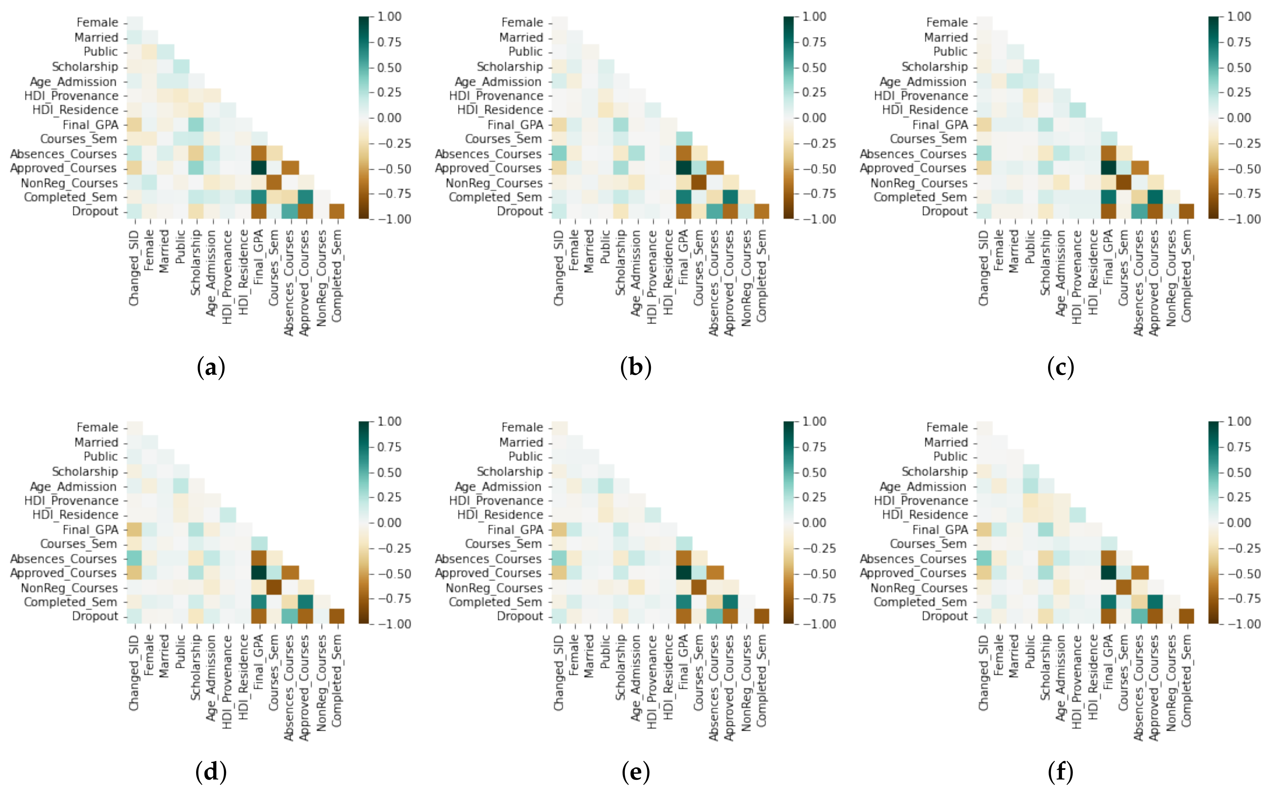
We used the correlational analysis of the variables involved to answer this question. Figure 2 shows the correlation matrices for each academic department. We represent positive correlations on the green scale, and the brown scale represents negative ones. As is evident, Completed_Sem has a strong negative correlation with Dropout in all cases. Furthermore, Dropout has a strong negative correlation with Final_GPA and Approved_Courses. However, Dropout and Absences_Courses have a moderate positive correlation.

In general, the correlation analysis is similar in all departments. Although a more detailed analysis, we found slight differences. In CS, we have a weak positive correlation between NonReg_Courses and Dropout. However, this correlation is almost null in the rest of the departments. In summary, we concluded from Figure 2 that the academic variables (Final_GPA and Approved_Courses) present a higher correlation with Dropout. In contrast, the socioeconomic (HDI_Provenance and HDI_Residence) and equity (Female) variables do not show a weak correlation in all cases. We concluded that these factors do not significantly influence predicting the dropout status.

6.2. RQ2: What Is the Most-Efficient Classification Machine Learning Method for the SDP Problem?

We utilized the Scikit-learn Python library to compute the classification probability. Now, we detail the best parameters for each classification algorithm employed in this work as follows:

• Logistic Regression (LR) considers C = 0.1.
• Support Vector Machine (SVM) considers C = 10 and gamma = 0.01.
• Gaussian Naive Bayes (GNB) considers a variance of smoothing equal to =0.001.
• K-Nearest Neighbor (KNN) considers seven neighbors.
• Decision Tree (DT) considers a minimum number of samples required to be at a leaf node equal to fifty and a maximum depth of the tree equal to nine.
• Random Forest (RF) considers a minimum number of samples required to be at a leaf node equal to fifty and a maximum depth of the tree equal to nine and does not use bootstrap.
• Multilayer Perceptron (MP) considers three layers in the sequence (13, 8, 4, 1), an activation function defined by tanh, and $\alpha$ = 0.001.
• Convolutional Neural Network (CNN) considers two layers in the sequence (13, 6, 1) and the activation functions ReLU and sigmoid.

The predictive capacity of these models was measured using Accuracy, AUC, and MSE, and these values are summarized in

Table 6. Evaluation metrics using classification algorithms. We highlight the best (in green) and worst (in brown) values by academic department.

Metrics	Department	LR	SVM	GNB	KNN	DT	RF	MLP	CNN
	Edu	0.855	0.860	0.817	0.791	0.860	0.862	0.830	0.913
	CS	0.829	0.833	0.823	0.809	0.839	0.859	0.818	0.987
Accuracy	Psy	0.883	0.882	0.847	0.872	0.865	0.895	0.873	0.946
	LPS	0.879	0.875	0.788	0.856	0.866	0.884	0.880	0.922
	EBS	0.858	0.864	0.822	0.845	0.856	0.868	0.852	0.908
	Eng	0.889	0.894	0.854	0.876	0.885	0.902	0.892	0.920
	Edu	0.913	0.914	0.908	0.898	0.890	0.931	0.890	0.936
	CS	0.908	0.909	0.908	0.875	0.895	0.921	0.892	0.884
AUC	Psy	0.940	0.939	0.917	0.930	0.928	0.954	0.935	0.937
	LPS	0.938	0.930	0.912	0.909	0.925	0.944	0.930	0.916
	EBS	0.919	0.926	0.906	0.907	0.921	0.938	0.919	0.918
	Eng	0.949	0.954	0.931	0.940	0.947	0.963	0.953	0.943
	Edu	0.145	0.140	0.183	0.209	0.140	0.138	0.170	0.065
	CS	0.171	0.167	0.177	0.109	0.161	0.141	0.182	0.012
MSE	Psy	0.117	0.118	0.153	0.128	0.135	0.105	0.127	0.043
	LPS	0.121	0.125	0.212	0.144	0.134	0.116	0.120	0.057
	EBS	0.142	0.136	0.178	0.155	0.144	0.132	0.148	0.069
	Eng	0.111	0.106	0.146	0.124	0.115	0.098	0.108	0.059

. We highlight the best evaluation metrics by coloring the cell green and the worst evaluation metrics in brown.

CNN presented the best results in most cases and obtained the highest accuracy in CS with (Accuracy = 0.987). Even in the other cases, the accuracy values are more significant than 0.9. However, CNN showed lower performance in some instances when we compared the AUC. Analyzing Psy, we found the highest accuracy value of 0.944, in contrast to what happened in CS, whose accuracy value is 0.921 and is the lowest. Evaluating the methods based on the AUC, we found that RF presents the best results in five of the six data subsets. From Table 6, we note that GNB showed the worst evaluation metrics in most cases. Finally, based on the experimentation presented above, we concluded that CNN is the best technique for the SDP problem employing classification algorithms.

6.3. RQ3: What Is the Most-Efficient Survival Analysis Method for the SDP Problem?

We employed survival analysis methods such as: the Cox Proportional Hazards model (CPH), Random Survival Forest (RSF), Conditional Survival Forest (CSF), and Multi-Task Logistic Regression (MTLR). In addition, variants of deep learning techniques such as Neural Multi-Task Logistic Regression model (N-MTLR), and Nonlinear Cox regression (DeepSurv) were implemented as well, and we compared them with the parametric models using the Gompertz and Weibull distributions.

We summarize in

Table 7. Evaluation metrics using survival machine learning methods. We highlight the best (in green) and worst (in brown) values by academic department.

Metrics	Department	Weibull	Gompertz	CPH	RSF	CSF	MTLR	N-MTLR	DeepSurv
	Edu	0.867	0.869	0.871	0.899	0.902	0.863	0.901	0.916
	CS	0.880	0.882	0.887	0.864	0.872	0.888	0.881	0.891
C-index	Psy	0.931	0.925	0.928	0.860	0.874	0.932	0.937	0.940
	LPS	0.911	0.911	0.915	0.882	0.904	0.909	0.918	0.923
	EBS	0.910	0.908	0.911	0.879	0.908	0.916	0.928	0.935
	Eng	0.933	0.931	0.936	0.899	0.924	0.941	0.949	0.952
	Edu	0.094	0.099	0.085	0.109	0.093	0.082	0.082	0.081
	CS	0.105	0.105	0.095	0.117	0.105	0.086	0.089	0.087
IBS	Psy	0.070	0.077	0.060	0.085	0.073	0.053	0.045	0.048
	LPS	0.081	0.087	0.074	0.092	0.080	0.068	0.066	0.063
	EBS	0.081	0.087	0.075	0.086	0.075	0.067	0.059	0.054
	Eng	0.070	0.076	0.062	0.080	0.065	0.049	0.043	0.041
	Edu	0.083	0.054	0.042	0.074	0.065	0.088	0.096	0.040
	CS	0.111	0.07	0.043	0.122	0.093	0.082	0.092	0.034
MSE	Psy	0.114	0.070	0.045	0.085	0.059	0.104	0.109	0.052
	LPS	0.107	0.070	0.047	0.081	0.052	0.091	0.094	0.036
	EBS	0.089	0.063	0.048	0.081	0.047	0.084	0.103	0.038
	Eng	0.112	0.076	0.050	0.095	0.053	0.101	0.110	0.041
	Edu	0.267	0.212	0.165	0.271	0.258	0.223	0.238	0.169
	CS	0.313	0.252	0.194	0.339	0.305	0.236	0.285	0.188
MAE	Psy	0.317	0.249	0.178	0.294	0.245	0.276	0.243	0.199
	LPS	0.303	0.245	0.176	0.285	0.217	0.247	0.215	0.158
	EBS	0.275	0.233	0.182	0.285	0.208	0.228	0.232	0.167
	Eng	0.312	0.258	0.171	0.307	0.227	0.228	0.229	0.166

the values of the C-index, IBS, MSE, and MAE. Similarly, the best metrics are colored green and the opposite case in brown. The PySurvival Python library calculates the survival probability, risk score, and metrics, and the visual representation of the survival curves was obtained with the Matplotlib Python library. The parameters employed for each method were the following:

• The parametric methods (Weibull and Gompertz) consider a learning rate equal to 0.01, an L2 regularization parameter equal to 0.001, the initialization method given by zeros, and the number of epochs equal to 2000.
• The Cox Proportional Hazards model CPH) considers a learning rate equal to 0.5 and an L2 regularization parameter equal to 0.01. The significance level $\alpha =0.95$, and the initialization method is given by zeros.
• Random Survival Forest (RSF) considers two-hundred trees, a maximum depth equal to twenty, the minimum number of samples required to be at a leaf node equal to ten, and the percentage of original samples used in each tree building equal to 0.85.
• Conditional Survival Forest (CSF) considers two-hundred trees, a maximum depth equal to five, the minimum number of samples required to be at a leaf node equal to twenty, the percentage of original samples used in each tree building equal to 0.65, and the lower quantile of the covariate distribution for splitting equal to 0.1.
• Multi-Task Logistic Regression (MTLR) considers twenty bins, a learning rate equal to 0.001, and the initialization method given by tensors with an orthogonal matrix.
• Neural Multi-Task Logistic Regression (N-MTLR) considers three layers with the activation functions defined by ReLU, tanh, and sigmoid. Furthermore, MTLR uses 120 bins, a smoothing L2 equal to 0.001, and five-hundred epochs, and tensors comprise the initialization method with an orthogonal matrix.
• Nonlinear Cox regression (DeepSurv) considers three layers with the activation functions defined by ReLU, tanh, and sigmoid. Furthermore, DeepSurv employs a learning rate equal to 0.001, and Xavier’s uniform initializer is the initialization method.

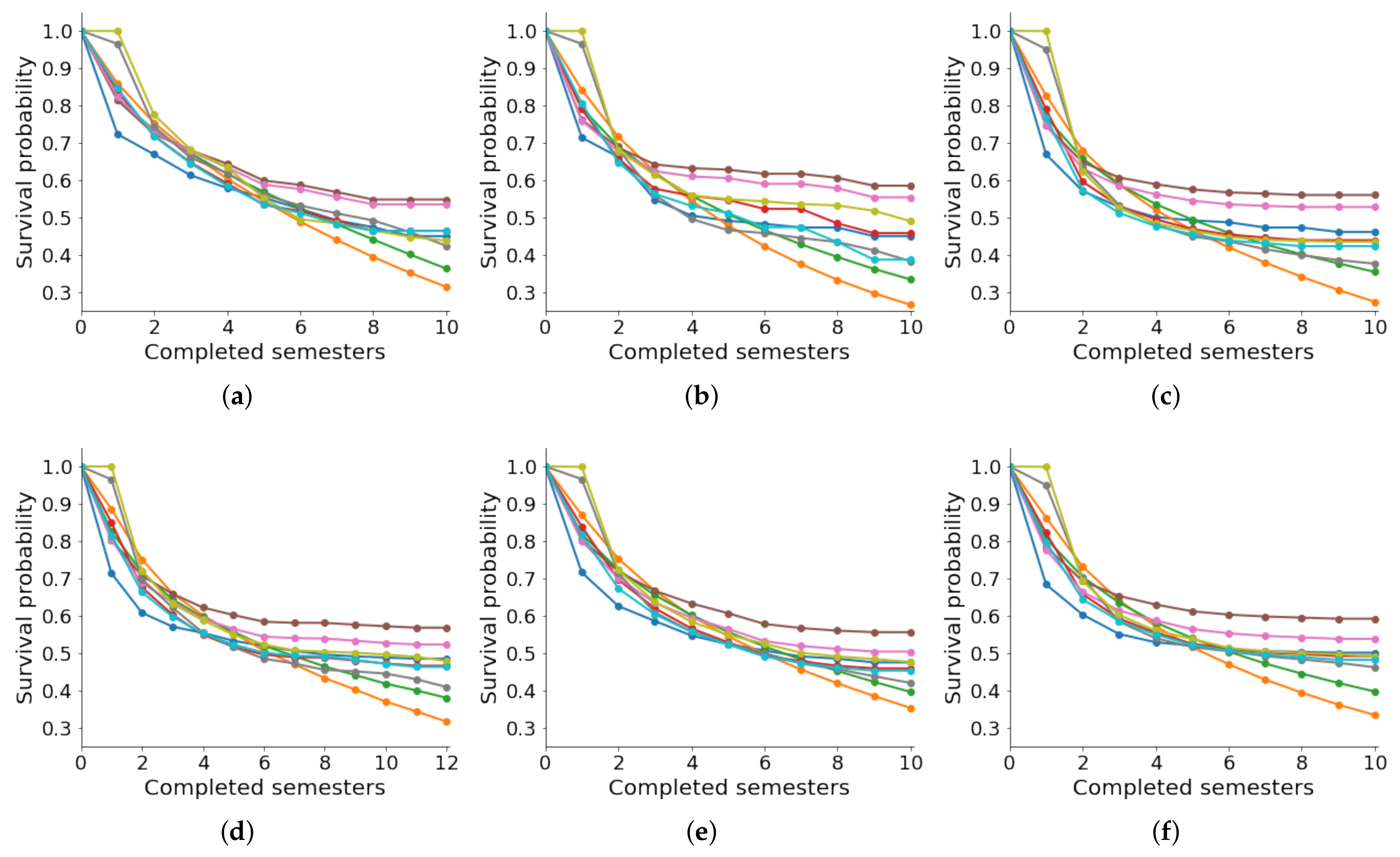
In almost all cases, DeepSurv presents the best results. Analyzing Psy, DeepSurv does not perform well when evaluating the IBS and MSE metrics. In most cases, the C-index value is higher than 0.90, which is a good indicator. However, this does not occur when analyzing CS (C-index = 0.891). In contrast, MSE = 0.0034, which is the best value compared to the other departments.

C-index and IBS are the metrics of survival analysis and are not usually good predictive indicators. For this reason, in our research, we employed regression metrics such as MSE and MAE to evaluate the survival curves for each department. Figure 3 illustrates the actual survival curves (in blue ) by each academic department.

We employed the KM estimator to compute such curves and compared them with the predicted survival curves for the other methods. In general, parametric models such as Weibull and Gompertz do not present good results. Visually, we noticed that these methods predict lower chances of survival. In contrast, RSF and CSF have high survival probabilities; however, their approximation to the actual survival curve is very distant. MTLR and N-MTLR are very close to the actual survival curve; however, the estimation in the first two semesters is very poor. The models that present the best results when predicting the survival curve are CPH and DeepSurv. Finally, we concluded that DeepSurv is the best model in this context. However, predicting the survival probability during the first two semesters is not good for all methods.

6.4. RQ4: How Influential Is Academic Performance in Estimating Dropout Risk?

In this section, we analyze the influence of academic performance based on the level of risk of dropping out. We first calculated each predictor variable’s importance percentage and detail it in

Table 8. Importance percentage of the predictor variables. We highlight the best (in green) and worst (in brown) percentage values by academic department.

Attribute Name	Edu	CS	Psy	LPS	EBS	Eng
Changed_SID	4.65%	9.88%	10.4%	15.66%	17.87%	15.92%
Female	0%	0%	0%	2.88%	1.28%	0.68%
Married	0%	0%	2.01%	0%	0%	0%
Public	0%	0%	0.54%	0%	2.52%	2.98%
Scholarship	3.27%	2.67%	2.36%	4.33%	0%	8.13%
Age_Admission	2.41%	3.09%	0%	1.47%	0.23%	2%
HDI_Provenance	0%	0.03%	0%	0%	0.14%	2.83%
HDI_Residence	0%	4.81%	2.17%	0%	0.66%	0.36%
Final_GPA	29.04%	19.18%	24.55%	19.85%	21.16%	17.19%
Courses_Sem	10.89%	11.77%	11.7%	11.66%	12.09%	9.78%
Absences_Courses	13.83%	12.33%	12.47%	10.04%	9.18%	9.02%
Approved_Courses	25.54%	24.15%	25.84%	22.24%	21.92%	21.55%
NonReg_Courses	10.66%	12.11%	7.96%	11.87%	12.94%	9.56%

. Some demographic attributes have very little influence, such as Female, Married, Public, Age_Admission, HDI_Provenance, and HDI_Residence. We found a moderate impact with the variable Changed_SID; however, its percentage of importance depends on the department. For example, in Edu, the importance percentage of Changed_SID is 4.65%; in contrast, 17.87% is the importance level of Changed_SID in EBS.

The highest rates obtained in each department are highlighted in green, thus obtaining which variables associated with academic performance Approved_Courses and Final_GPA are the most influential. In most cases, Approved_Courses has the highest percentage of importance, and it is only lower than Final_GPA when we analyze Edu. These results corroborate the strong negative correlation of these variables with Dropout, as illustrated in Figure 2. Although this confirms a strong and meaningful impact of the academic variables, we do not know to what extent they influence the different departments.

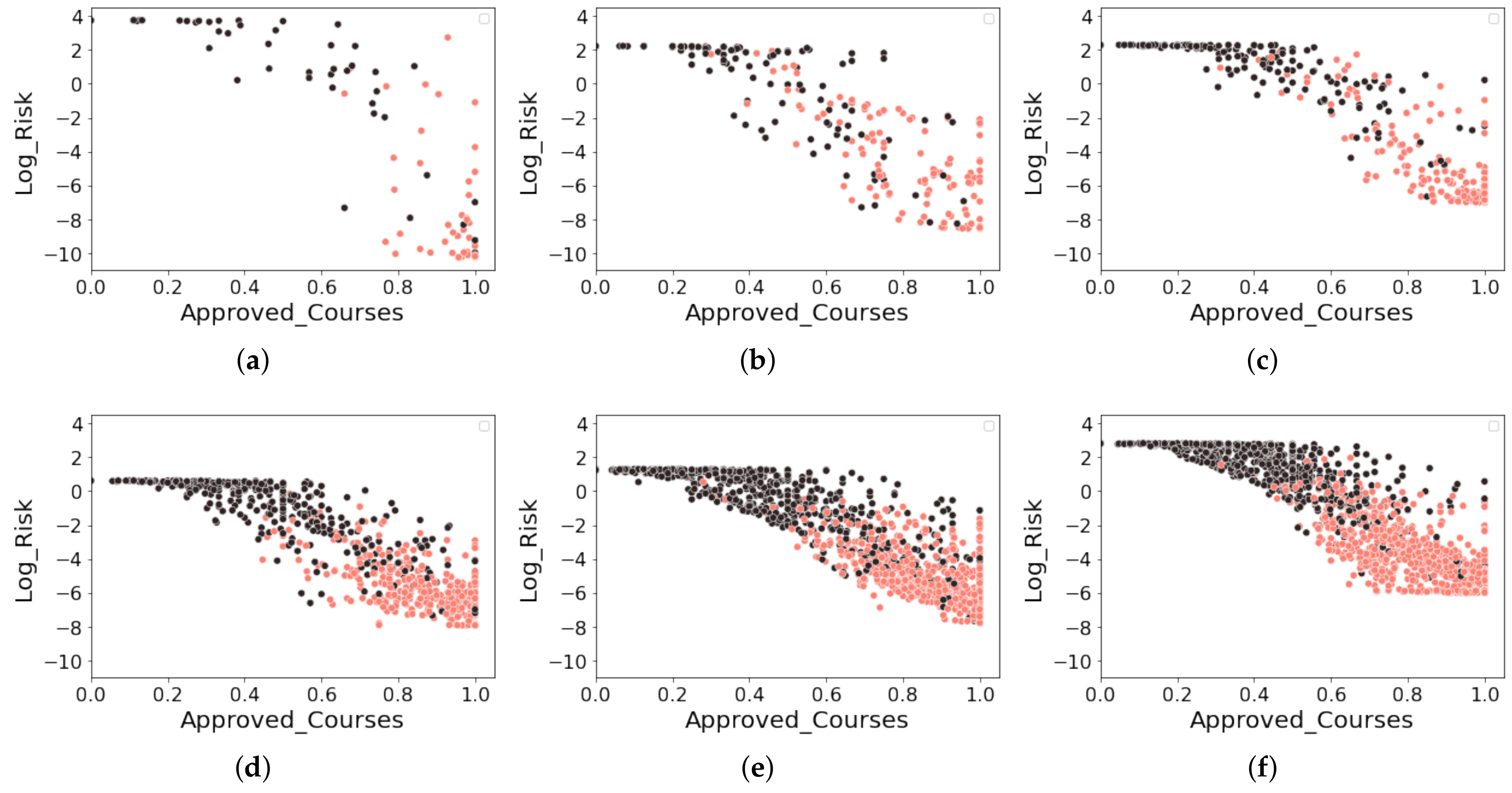
Since DeepSurv was the best method for predicting student dropout in the survival format, we used it in the test sets to predict the risk score defined in (7). Therefore, we implement in Figure 4 various scatter plots to visualize the data distribution according to the proportion of approved courses (Approved_Courses) and the logarithm of the risk score, denoted by Log_Risk. For each subfigure, we define the x-axis as Approved_Courses and the y-axis as Log_Risk and color the point data according to the dropout’s status (Dropout). We highlight a student who has dropped out in black, while a student who has not dropped out is in pink.

As can be visually identified, a negative correlation exists between Approved_Courses and Log_Risk. We note a particular case in Edu in which all students with a proportion of approved courses less than 0.6 ($\mathtt{Approved}\_\mathtt{Courses}<0.6$) are all dropouts. However, this situation did not occur in other departments. With this brief analysis, we found indications that the impact of Approved_Courses is more influential in Education compared to the other departments. Furthermore, each department’s predicted values of Log_Risk differ considerably. In Edu, we found on the y-axis that the range of values assumed by Log_Risk goes from −10 to 4. However, this does not happen in the other departments, which generally range between −8 and 2.

On the other hand, in STEM programs such as CS and Eng, we found higher numbers of students who did not drop out despite having a high failure rate in the courses (i.e., Approved_Courses < 0.6). Generally, these programs are challenging due to their predominant curricula based on exact sciences in the first semesters. Moreover, there is a tendency to normalize the effect of failing some courses. Complementing our analysis with the values of NonReg_Courses from Table 5 and Table 8, we deduced that many students in STEM programs take courses in non-regular semesters to recover the failed courses. This is usually considered a characteristic of the persistence of these students.

More traditional programs, such as LPS and EBS, have a very similar behavior for the data dispersion and the range of predicted values of Log_Risk. In this context, we can complement the persistence of these students with the variable Changed_SID. It does not have a more prominent percentage presence as described in Table 4; the importance of the variable in the model is one of the most relevant, as revealed in Table 8.

Although we noticed that Edu behaves differently from the others, we can show that Psy is possibly the most similar to Edu. Observing the importance percentages of Final_GPA computed in Table 8 in both cases, we note that these values exceed 24%, which are the highest values in our dataset. Unlike measuring the influence of economic variables from the perspective of approved courses, in Edu and Psi, we found that the grades are decisive, which led us to think that students in these programs generally have higher GPAs than those in other careers. Due to the wide granting of school scholarships, as reflected in Education, more than 12% of our sample has a scholarship. Generally, scholarship students seek to maintain high grades to avoid losing this study funding. On the other hand, in Edu and Psy, we show high importance to the hours of absence; that is, the impact of being hours absent from courses (Absences_Courses) in these careers is a very relevant aspect if we compare it with the other departments.

Finally, we concluded from our analysis that the impact of academic variables is decisive in predicting the risk of dropping out. However, the effect that this generates is different in each department. Understanding this analysis requires a global study of the importance of the attributes and a complementary analysis based on statistical tools.

7. Discussion

Our research sought to determine efficient and customized solution strategies best suited to student dropout prediction, employing machine learning and survival analysis models and their deep variants. Before evaluating these computational techniques, a descriptive analysis was necessary to have a preliminary idea of the significant attributes, their distribution, and their correlation in each department’s given sample data.

From this perspective, Edu presented a data distribution quite dissimilar from the rest, as shown in Table 4 and Table 5. Furthermore, when calculating the correlation rates illustrated in Figure 2, we determined that academic variables such as Final_GPA and Approved_Courses stand out with a strong negative correlation with the event variable given by Dropout, as we can see in Figure 2. Similarly, we noticed a robust negative correlation between Dropout and Completed_Sem (see Figure 2). Therefore, based on these values, it is evident that the academic and temporal variables have a predominant role in predicting student dropout, as various works in the literature have concluded [5,11,23,40].

The correlational analysis presented in Section 6.1 supports the feature selection process, allowing us to generate calculated attributes instead of using raw data. For instance, we employed a proportion of approved courses concerning the total number of enrolled courses (Approved_Courses) instead of the total number of approved courses solely. Using this approach, we aimed to mitigate the temporal influence of an attribute. This preliminary step is decisive for evaluating the classification and survival methods jointly.

Using classification models, presented in Section 6.2, RF and CNN stood out, as shown in Table 6. Evaluating Accuracy and SME, we found that CNN performed better on all data samples. However, RF presents the best AUC value in almost all of them. The opposite case occurs with GNB and KNN, while in the survival analysis methods, detailed in Section 6.3, DeepSurv was the one with the best predictive capacity; see Table 7. Then, we verified that the deep variants in both contexts presented robust results.

We evidence that, despite the substantial difference in the formulation of both approaches, the main problem lies mainly in defining the objective variable (Y), — i.e., $Y=\mathtt{Dropout}$ for the classification algorithms and $Y=(\mathtt{Dropout},\mathtt{Completed}\_\mathtt{Sem})$ for the survival analysis methods. In both approaches, we utilized the same predictor variables. It is not enough to predict which students will drop out, but to understand when the dropout will occur. Then, the application of these techniques should be exploited in a complementary fashion. For instance, when visualizing the prediction of the survival curves given in Figure 3, we obtained a low prediction during the first two semesters. This may be due to an incorrect choice of an academic program or a deficient academic background in high schools. Analyses such as ours will enable educational managers to understand the dropout problem better, predict who will drop out and when, and thus, make the right decisions over time. Statistical evidence reveals that academic variables are decisive in predicting student dropout, as detailed in Section 6.4. The opposite case occurs with socioeconomic and equity variables. Possibly, some cases of dropout are caused by variables not considered in this work, such as the familiar/professional environment and psychological/emotional condition. However, we generated efficient models from available data from most universities globally.

Finally, this analysis must be carried out carefully and in collaboration with educational managers to obtain constant feedback. We also must highlight that not all the undergraduate programs have the same behavior. Dropout conditions are different for each program. Each dropout case must be analyzed individually, as it depends not only on the individual, but also on the program he/she is studying. The generalization of the rule is clearly a mistake that we must avoid.

8. Conclusions

This work focused on analyses of a case study in a Latin American university to find an efficient computational mechanism for predicting student dropout. Furthermore, our analysis explores two approaches to addressing the SDP problem: (i) as a classification task to expect who will drop out and (ii) as a survival analysis that seeks to determine when the dropout will occur. We employed the same set of attributes in both prediction strategies.

In predicting who will drop out, we found that RF and CNN presented the best results in the evaluation metrics given by the Accuracy, AUC, and MSE. The opposite happens with more basic classification techniques (GNB and KNN). However, implementing these techniques differs considerably depending on the analyzed academic department. For example, we obtained higher AUC values in Engineering (↑; see Table 6) than in Education (↓; see Table 6). However, this analysis alone does not allow a general overview to make decisions over time. Applying the survival analysis techniques enabled us to identify when the dropout occurs. Our experimentation showed that DeepSurv is the technique that has the best prediction results (↑; see Table 7). Although the evaluation metrics for survival are reasonable, we found great difficulty predicting dropout in the first semesters, as we visualized when predicting the survival curves for the test sets. The possible causes of dropout in the first semesters are widely diverse. They may be related to aspects of motivation and adaptation to university life and low academic background, making it challenging to have an excellent academic performance. Using the temporal approach, we found that the academic variables have a crucial determining role. It is also evident in the correlational analysis defined in the exploratory data analysis.

Our research included a detailed analysis of the influence of academic variables in predicting the level of risk of dropping out using the most-robust survival technique, DeepSurv. Here, we found that the impact generated by one academic department is not always similar for all of them. This work concisely evaluated various computational techniques, revealing an appropriate parameter setup. The clarity of our proposal will allow the scientific community to reproduce it in the same educational context (e.g., studying different academic phenomena such as student retention) and adapt it to multiple other contexts that seek to predict who, when, and why a specific event would occur.

References

1. Bernardo, A.; Esteban, M.; Fernández, E.; Cervero, A.; Tuero, E.; Solano, P. Comparison of Personal, Social and Academic Variables Related to University Drop-out and Persistence. Front. Psychol. 2016, 7, 1610. [Google Scholar] [CrossRef]
2. Tinto, V. Dropout from Higher Education: A Theoretical Synthesis of Recent Research. Rev. Educ. Res. 1975, 45, 89–125. [Google Scholar] [CrossRef]
3. Nicoletti, M. Revisiting the Tinto’s Theoretical Dropout Model. High. Educ. Stud. 2019, 9, 52–64. [Google Scholar] [CrossRef]
4. Gutierrez-Pachas, D.A.; Garcia-Zanabria, G.; Cuadros-Vargas, A.J.; Camara-Chavez, G.; Poco, J.; Gomez-Nieto, E. How Do Curricular Design Changes Impact Computer Science Programs?: A Case Study at San Pablo Catholic University in Peru. Educ. Sci. 2022, 12, 242. [Google Scholar] [CrossRef]
5. Rovira, S.; Puertas, E.; Igual, L. Data-driven system to predict academic grades and dropout. PLoS ONE 2017, 12, 171–207. [Google Scholar] [CrossRef] [PubMed]
6. Da Costa, F.J.; de Souza Bispo, M.; de Cássia de Faria Pereira, R. Dropout and retention of undergraduate students in management: A study at a Brazilian Federal University. RAUSP Manag. J. 2018, 53, 74–85. [Google Scholar] [CrossRef]
7. Del Bonifro, F.; Gabbrielli, M.; Lisanti, G.; Zingaro, S.P. Student Dropout Prediction. In Artificial Intelligence in Education, 21st International Conference, AIED 2020, Ifrane, Morocco, 6–10 July 2020, Proceedings, Part I 21; Springer: Berlin/Heidelberg, Germany, 2020; pp. 129–140. [Google Scholar]
8. Mduma, N.; Kalegele, K.; Machuve, D. A Survey of Machine Learning Approaches and Techniques for Student Dropout Prediction. Data Sci. J. 2019, 18, 14. [Google Scholar] [CrossRef]
9. Prenkaj, B.; Velardi, P.; Stilo, G.; Distante, D.; Faralli, S. A Survey of Machine Learning Approaches for Student Dropout Prediction in Online Courses. ACM Comput. Surv. 2020, 53, 57. [Google Scholar] [CrossRef]
10. De Oliveira, C.F.; Sobral, S.R.; Ferreira, M.J.; Moreira, F. How Does Learning Analytics Contribute to Prevent Students’ Dropout in Higher Education: A Systematic Literature Review. Big Data Cogn. Comput. 2021, 5, 64. [Google Scholar] [CrossRef]
11. Aulck, L.S.; Nambi, D.; Velagapudi, N.; Blumenstock, J.; West, J. Mining University Registrar Records to Predict First-Year Undergraduate Attrition. In Proceedings of the 12th International Conference on Educational Data Mining, Montreal, QC, Canada, 2–5 July 2019; International Educational Data Mining Society: Worcester, MA, USA, 2019. [Google Scholar]
12. Ameri, S.; Fard, M.J.; Chinnam, R.B.; Reddy, C.K. Survival Analysis Based Framework for Early Prediction of Student Dropouts. In Proceedings of the 25th ACM International on Conference on Information and Knowledge Management, Indianapolis, IN, USA, 24–28 October 2016; Association for Computing Machinery: New York, NY, USA, 2016; pp. 903–912. [Google Scholar]
13. Wang, P.; Li, Y.; Reddy, C.K. Machine Learning for Survival Analysis: A Survey. ACM Comput. Surv. 2019, 51, 110. [Google Scholar] [CrossRef]
14. Spooner, A.; Chen, E.; Sowmya, A.; Sachdev, P.; Kochan, N.A.; Trollor, J.; Brodaty, H. A comparison of machine learning methods for survival analysis of high-dimensional clinical data for dementia prediction. Sci. Rep. 2020, 10, 20410. [Google Scholar] [CrossRef] [PubMed]
15. Katzman, J.L.; Shaham, U.; Cloninger, A.; Bates, J.; Jiang, T.; Kluger, Y. DeepSurv: Personalized treatment recommender system using a Cox proportional hazards deep neural network. BMC Med. Res. Methodol. 2018, 18, 24. [Google Scholar] [CrossRef] [PubMed]
16. Yu, C.N.; Greiner, R.; Lin, H.C.; Baracos, V. Learning Patient-Specific Cancer Survival Distributions as a Sequence of Dependent Regressors. In Proceedings of the Advances in Neural Information Processing Systems; Shawe-Taylor, J., Zemel, R., Bartlett, P., Pereira, F., Weinberger, K., Eds.; Curran Associates, Inc.: Red Hook, NY, USA, 2011; Volume 24. [Google Scholar]
17. Fotso, S. Deep Neural Networks for Survival Analysis Based on a Multi-Task Framework. arXiv 2018, arXiv:1801.05512. [Google Scholar]
18. Ishwaran, H.; Kogalur, U.B.; Blackstone, E.H.; Lauer, M.S. Random survival forests. Ann. Appl. Stat. 2008, 2, 841–860. [Google Scholar] [CrossRef]
19. Wright, M.N.; Dankowski, T.; Ziegler, A. Unbiased split variable selection for random survival forests using maximally selected rank statistics. Stat. Med. 2017, 36, 1272–1284. [Google Scholar] [CrossRef] [PubMed]
20. Pan, F.; Huang, B.; Zhang, C.; Zhu, X.; Wu, Z.; Zhang, M.; Ji, Y.; Ma, Z.; Li, Z. A survival analysis based volatility and sparsity modeling network for student dropout prediction. PLoS ONE 2022, 17, e0267138. [Google Scholar] [CrossRef] [PubMed]
21. Lee, C.; Zame, W.; Yoon, J.; van der Schaar, M. DeepHit: A Deep Learning Approach to Survival Analysis with Competing Risks. In Proceedings of the AAAI Conference on Artificial Intelligence, New Orleans, LA, USA, 2–7 February 2018; Volume 32. [Google Scholar]
22. Hu, S.; Fridgeirsson, E.A.; van Wingen, G.; Welling, M. Transformer-Based Deep Survival Analysis. In Proceedings of the AAAI Spring Symposium 2021 (SP-ACA), Palo Alto, CA, USA, 22–24 March 2021. [Google Scholar]
23. Gutierrez Pachas, D.A.; Garcia-Zanabria, G.; Cuadros-Vargas, A.J.; Camara-Chavez, G.; Poco, J.; Gomez-Nieto, E. A comparative study of WHO and WHEN prediction approaches for early identification of university students at dropout risk. In Proceedings of the 2021 XLVII Latin American Computing Conference (CLEI), Cartago, Costa Rica, 25–29 October 2021; pp. 1–10. [Google Scholar]
24. Garcia-Zanabria, G.; Gutierrez-Pachas, D.A.; Camara-Chavez, G.; Poco, J.; Gomez-Nieto, E. SDA-Vis: A Visualization System for Student Dropout Analysis Based on Counterfactual Exploration. Appl. Sci. 2022, 12, 5785. [Google Scholar] [CrossRef]
25. Platt, A.; Fan-Osuala, O.; Herfel, N. Understanding and Predicting Student Retention and Attrition in IT Undergraduates. In Proceedings of the 2019 on Computers and People Research Conference, SIGMIS-CPR’19, Nashville, TN, USA, 20–22 June 2019; Association for Computing Machinery: New York, NY, USA, 2019; pp. 135–138. [Google Scholar]
26. Vásquez Verdugo, J.; Miranda, J. Student Desertion: What Is and How Can It Be Detected on Time? In Data Science and Digital Business; García Márquez, F.P., Lev, B., Eds.; Springer: Cham, Switzerland, 2019; pp. 263–283. [Google Scholar]
27. Tanner, T.; Toivonen, H. Predicting and preventing student failure - using the k-nearest neighbour method to predict student performance in an online course environment. Int. J. Learn. Technol. 2010, 5, 356–377. [Google Scholar] [CrossRef]
28. Medina, E.C.; Chunga, C.B.; Armas-Aguirre, J.; Grandón, E.E. Predictive model to reduce the dropout rate of university students in Perú: Bayesian Networks vs. Decision Trees. In Proceedings of the 2020 15th Iberian Conference on Information Systems and Technologies (CISTI), Sevilla, Spain, 24–27 June 2020; pp. 1–7. [Google Scholar]
29. Siri, D. Predicting Students’ Dropout at University Using Artificial Neural Networks. Ital. J. Sociol. Educ. 2015, 7, 225–247. [Google Scholar]
30. Buchhorn, J.; Wigger, B.U.; Wigger, B.U. Predicting Student Dropout: A Replication Study Based on Neural Networks; CESifo Working Paper No. 9300; Munich Society for the Promotion of Economic Research - CESifo GmbH: Munich, Germany, 2021. [Google Scholar]
31. Mezzini, M.; Bonavolontà, G.; Agrusti, F. Predicting university dropout by using convolutional neural networks. In Proceedings of the INTED2019 Proceedings, 13th International Technology, Education and Development Conference, IATED, Valencia, Spain, 11–13 March 2019; pp. 9155–9163. [Google Scholar]
32. Wu, N.; Zhang, L.; Gao, Y.; Zhang, M.; Sun, X.; Feng, J. CLMS-Net: Dropout Prediction in MOOCs with Deep Learning. In Proceedings of the ACM Turing Celebration Conference—China, ACM TURC’19, Chengdu, China, 17–19 May 2019; Association for Computing Machinery: New York, NY, USA, 2019. [Google Scholar]
33. Mubarak, A.A.; Cao, H.; Hezam, I.M. Deep analytic model for student dropout prediction in massive open online courses. Comput. Electr. Eng. 2021, 93, 107271. [Google Scholar] [CrossRef]
34. Zheng, P.; Yuan, S.; Wu, X. SAFE: A Neural Survival Analysis Model for Fraud Early Detection. In Proceedings of the Thirty-Third AAAI Conference on Artificial Intelligence and Thirty-First Innovative Applications of Artificial Intelligence Conference and Ninth AAAI Symposium on Educational Advances in Artificial Intelligence, AAAI’19/IAAI’19/EAAI’19, Honolulu, HI, USA, 27 January–1 February 2019. [Google Scholar]
35. Juajibioy, J.C. Study of University Dropout Reason Based on Survival Model. Open J. Stat. 2016, 6, 908–916. [Google Scholar] [CrossRef]
36. Csalódi, R.; Abonyi, J. Integrated Survival Analysis and Frequent Pattern Mining for Course Failure-Based Prediction of Student Dropout. Mathematics 2021, 9, 463. [Google Scholar] [CrossRef]
37. Cox, D.R. Regression Models and Life-Tables. J. R. Stat. Soc. Ser. B (Methodological) 1972, 34, 187–220. [Google Scholar] [CrossRef]
38. Bani, M.; Haji, M. College Student Retention: When Do We Losing Them? In Proceedings of the World Congress on Engineering and Computer Science, Tehran, Iran, 26–28 April 2017. [Google Scholar]
39. Agrusti, F.; Mezzini, M.; Bonavolontà, G. Deep learning approach for predicting university dropout: A case study at Roma Tre University. J. E-Learn. Knowl. Soc. 2020, 16, 44–54. [Google Scholar]
40. Rodríguez-Muñiz, L.J.; Bernardo, A.B.; Esteban, M.; Díaz, I. Dropout and transfer paths: What are the risky profiles when analyzing university persistence with machine learning techniques? PLoS ONE 2019, 14, e0218796. [Google Scholar] [CrossRef] [Green Version]
Figure 1. Considering students A, B, C, and D, we illustrate the (a) permanence times and (b) survival curves for each of them.
Education 13 00154 g001
Figure 2. Heat map of the correlations between the attributes for each department. We illustrate the positive correlations (in green scale) and negative correlations (in brown scale). (a) Education (Edu). (b) Computer Science (CS). (c) Psychology (Psy). (d) Law and Political Sciences (LPS). (e) Economic and Business Sciences (EBS). (f) Engineering (Eng).
Education 13 00154 g002
Figure 3. Comparison of predicted survival curves. The actual curve is displayed in blue (Education 13 00154 i001), while the predicting methods are: Weibull (Education 13 00154 i002), Gompertz (Education 13 00154 i003), CPH (Education 13 00154 i004), RSF (Education 13 00154 i005), CSF (Education 13 00154 i006), MTLR (Education 13 00154 i007), N-MTLR (Education 13 00154 i008), and DeepSurv (Education 13 00154 i009). (a) Education (Edu). (b) Computer Science (CS). (c) Psychology (Psy). (d) Law and Political Sciences (LPS). (e) Economic and Business Sciences (EBS). (f) Engineering (Eng).
Education 13 00154 g003
Figure 4. Scatter plot between the proportion of approved courses and the logarithm of the risk score. We highlight a student dropout in black (●), otherwise in pink (). (a) Education (Edu). (b) Computer Science (CS). (c) Psychology (Psy). (d) Law and Political Sciences (LPS). (e) Economic and Business Sciences (EBS). (f) Engineering (Eng).
Education 13 00154 g004