Climate Change Impact on Peruvian Biomes

Abstract

The biodiversity present in Peru will be affected by climatic and anthropogenic changes; therefore, understanding these changes will help generate biodiversity conservation policies. This study analyzes the potential distributions of biomes (B) in Peru under the effects of climate change. The evaluation was carried out using the random forest (RF) method, six bioclimatic variables, and digital topography for the classification of current B in Peru. Subsequently, the calibrated RF model was assimilated to three downscaled regional climate models to project future B distributions for the 2035–2065 horizon. We evaluated possible changes in extension and elevation as well as most susceptible B. Our projections show that future scenarios agreed that 82% of current B coverage will remain stable. Approximately 6% of the study area will change its current conditions to conditions of higher humidity; 4.5% will maintain a stable physiognomy, but with an increase in humidity; and finally, 6% will experience a decrease in humidity but maintain its appearance. Additionally, glaciers and swamps are indicated as the most vulnerable B, with probable losses greater than 50% of their current area. These results demonstrate the need to generate public policies for the adaptation and mitigation of climate effects on B at a national scale.

1. Introduction

There is complex spatial and temporal variability in the existing vegetation on continents, which influences the resources available to support human well-being, biodiversity, and the biogeochemical cycle [1,2,3]. Climate and vegetation interact bidirectionally on many temporal and spatial scales; a clear manifestation of this interaction is the global pattern of vegetation cover and climate. Thus, climate can be considered the most influential factor in the distribution of vegetation and its characteristics on a global scale [4]. The ecological units that describe these vegetation variabilities in an organized manner are called biomes. Biomes are defined as similar geographic regions where living organisms with physiologically common characteristics are well adapted and strongly correlated with the regional climate [5]. These units are generally defined at large scales grouping similar ecological units.

With the B presenting a close relationship with climate, there are different models that explicitly incorporate climate variables such as Holdridge [6], who produced a life zones system scheme (B) that describes large vegetation formations described by climatic variables: precipitation, temperature, and potential evapotranspiration. Walter [7] similarly defined the B in terms of the climatic zone they occupy (zonobiomes), with modifications that include soils and orographic characteristics. Recently, the remote sensing (RS) of terrestrial coverage with satellites has allowed the creation of new B distribution maps [2] where the boundaries between the vegetation units are ostensibly defined objectively [8].

Based on these RS data, the evaluation of the changes has traditionally been performed with bioclimatic envelope models (BEMs) or with dynamic global vegetation models (DGVMs) [9,10]. The first is a correlative approach based on a strong relationship between the current climate and the distribution of vegetation, while the second is more realistic due to the consideration of ecological processes. The DGVM requires more information for their calibration, so it is linked to greater uncertainties in the estimates of their parameters. Meanwhile, BEM only requires climate information, which makes it more suitable for measuring the effects of climate change in developing countries where data are limited [11]. BEMs are based on statistical techniques or machine learning (ML) models. In recent years, with the increase in information on spatiotemporal forcing factors for determining B, BEM models have become more commonly used in ecology [11,12,13].

The B in Peru is quite variable, as are the existing climates in Peru; an approximation of them are continental ecosystems. A recent study of the Ministry of the Environment of Peru [14] identified 36 continental ecosystems in Peru, of which 11 were in the tropical forest region, 3 were in the Yunga region, 11 were in the Andean region, 9 were in the coastal region, and 2 were aquatic ecosystems. Since the B in Peru are linked to the climate and other factors such as phenological behavior and especially recently to changes in land use and vegetation cover, they are prone to changes, especially at more local scales [15]. It is estimated that by the end of the 21st century, warming in South America will increase by over 2 °C compared to historical records. Precipitations present greater variability in their future projections but suggest decreases in the Amazon and in Southern South America and increases in the Northern Andes [16]. Additionally, it is expected that as a result of these climatic changes, the B, considering the different future scenarios, between 5% and 6% of the total vegetation area in Latin America, will undergo changes towards the end of the 21st century [17].

In this context, by varying the climate, changes are inferred in the spatial distribution of the biomes that will lead to extinctions and diversification of species due to a faster migration rate [12]. In the case of Peru, studies have been conducted in the Andes; for example, Tovar et al. [18], who focuses on the Andean part of Peru, finds that only between 13% and 17% of the Andean region will exhibit significant changes in their B for the 2010–2039 and 2040–2069 horizons, with glaciers, paramos, and evergreen montane forests being the most threatened B. Bax et al. [19] reviews the implications of climate change in conservation plans since protected areas located in montane forests would be affected. Ramirez–Villegas et al. [20] projects that by 2050, the paramos and punas of the tropical Andes will have a reduction in their species and high rates of species alteration, with the most affected population being located between 800–1500 amsl. However, studies that encompass Peru as a whole have not been reported in the literature.

This study tries to answer the following questions: (1) How reliable does RF reproduce current biomes? (2) What is the impact of climate change (2035–2065) on the distribution of biomes in Peru? The novelty of this document is that it includes for the first time the entire Peruvian territory to estimate the biomes in Peru and evaluate the impact of climate change for the period 2035–2065 using future scenarios based on regional climate models for Peru.

2. Materials and Methods

The study area covers the entire region of Peru, located in the center-west of South America from latitudes 0° to 18° S and longitudes 68° to 82° W. The total area is approximately 1.27 million km² and covers extremely variable regions with different precipitation regimes. Climate variability is due to the complex orography of the Andes, the cold system of the Humboldt current, and the El Niño phenomenon [21,22]. According to Olson et al. [3], there are six types of biomes in Peru: tropical forest; tropical and subtropical broadleaf forests; tropical and subtropical dry broadleaf forests; savanna; deserts and xeric shrublands; grasslands; and montane shrublands. However, given the importance of some ecosystems for conservation planning, in this study, we used the biomes defined by Tovar et al. [18] in the tropical Andes with a slight modification of the rainforest area. The biomes defined are (1) evergreen montane forest (EMF), (2) seasonally dry tropical montane forest (SDTF), (3) humid puna (HP), (4) paramo (P), (5) montane shrubland (MS), (6) xeric pre-puna (PP), (7) glaciers (GC), (8) xeric puna (XP), (9) Yunga forest (YF), and (10) swamp (SW). The present configuration of the B was obtained by grouping the National Map of Ecosystems of Peru prepared by the Ministry of the Environment (Ministerio del Ambiente—MINAM) [14] using the biome classifications described.

Table 1. Distribution of biomes in Peru, percentage of coverage area, type of predominant ecological structure, and relative humidity level.

Peruvian Biomes	Area %	Plant Life Form	Humidity Level
EMF	42.44	forest	8
SDTF	2.42	forest	7
HP	12.84	grassland	4
P	1.08	grassland	5
MS	8.06	shrubland	6
PP	5.85	desert	1
GC	2.32	desert	2
XP	0.91	grassland	3
YF	13.53	forest	7
SW	4.84	forest	9

shows the percentage of area occupied by each biome in Peru while Figure 3 shows the present spatial distribution. In addition, a column was added indicating the relative humidity level on a scale from 1 to 10; 1 being a very dry biome and 10 a very humid biome [18].

2.1. Precipitation and Temperature

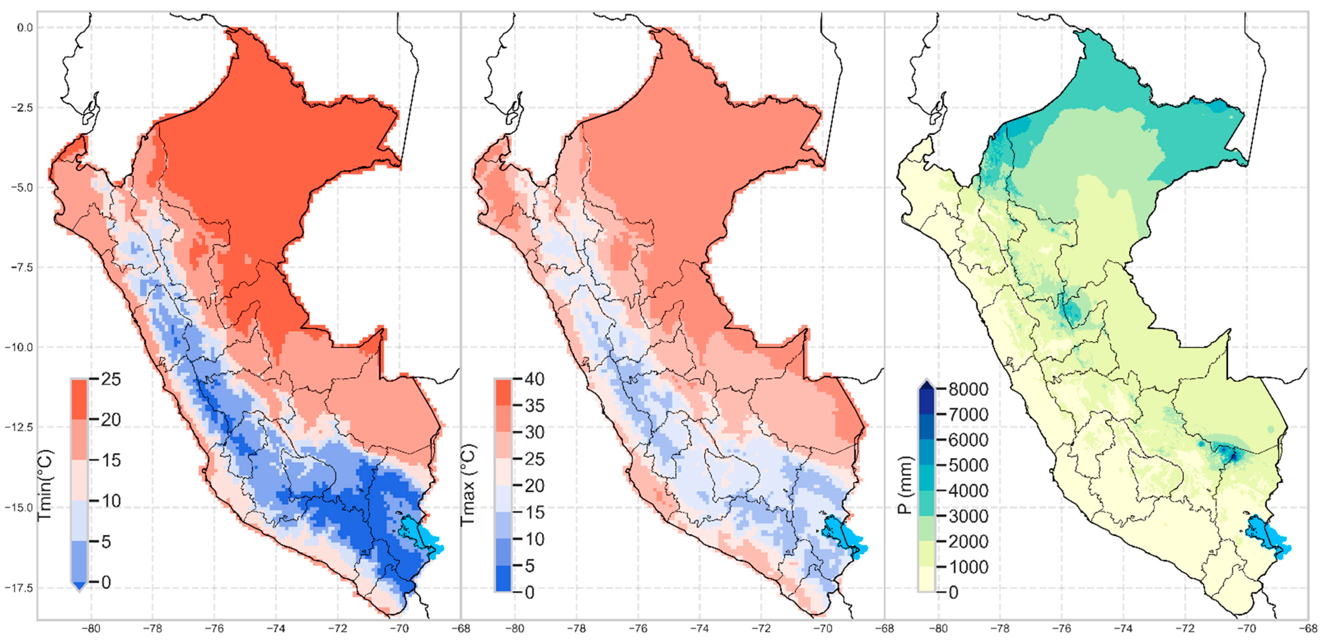
The gridded climatological data of precipitation and temperatures (minimum and maximum) were generated from the mixture of data from conventional climatological stations and continuous covariates in space. These products are found at a time scale of monthly climatology (1981–2010) and spatially at a resolution of 200 m² [23].

To generate precipitation data, 654 stations were used. The data cover areas of Peru, Colombia, Ecuador, Bolivia, and Brazil. Precipitation was interpolated using the Shuttle Radar Topography Mission (SRTM) digital elevation model as covariates; the global precipitation product Climate Hazard Infrared Precipitation with Stations (CHIRPS) version 2 [24]; and geographic coordinates (latitude and longitude). Finally, a multiple linear regression model (R) plus a residual inverse distance weighted (RIDW) interpolation was used to perform the mixture and generate these climatological maps.

For the maximum and minimum temperatures, RIDW was used considering the SRTM covariates geographic coordinates and soil surface temperature, where the latter was obtained from the moderate-resolution imaging spectroradiometer (MODIS) product MOD11A2 day/night [25]. A total of 442 weather stations were used, also considering stations located in neighboring countries.

To date, these weather grid data are the ones that have been used by most stations in their construction compared to other previous products in Peru [23,26]. Statistical validations and focus group with contributions from experts were carried out for final approval. The spatial distribution of the climatologies can be observed in Figure 1.

2.2. Bioclimatic and Geographic Variables

For the creation of the B classification model, bioclimatic variables (BVs) were used. In this regard, in the first phase, 19 BVs were defined by WorldClim (

Table A1. Bioclimatic variables.

Bioclimatic variables

BIO1 = Annual Mean Temperature

BIO2 = Mean Diurnal Range (Mean of monthly (max temp—min temp))

BIO3 = Isothermality (BIO2/BIO7) (×100)

BIO4 = Temperature Seasonality (standard deviation ×100)

BIO5 = Max Temperature of Warmest Month

BIO6 = Min Temperature of Coldest Month

BIO7 = Temperature Annual Range (BIO5-BIO6)

BIO8 = Mean Temperature of Wettest Quarter

BIO9 = Mean Temperature of Driest Quarter

BIO10 = Mean Temperature of Warmest Quarter

BIO11 = Mean Temperature of Coldest Quarter

BIO12 = Annual Precipitation

BIO13 = Precipitation of Wettest Month

BIO14 = Precipitation of Driest Month

BIO15 = Precipitation Seasonality (Coefficient of Variation)

BIO16 = Precipitation of Wettest Quarter

BIO17 = Precipitation of Driest Quarter

BIO18 = Precipitation of Warmest Quarter

BIO19 = Precipitation of Coldest Quarter

) [27]. To estimate the BV, the dismo package of the R programming language was used [28], as well as the historical climatology 1981–2010 of precipitation—temperatures described in the previous section. Once the BVs were calculated, we proceeded to select the most independent ones by filtering through a Pearson correlation matrix. By means of this matrix, only the BVs that presented a correlation lower than 90% were selected. The selected BVs were mean annual temperature, monthly temperature range, isothermality, temperature seasonality, annual precipitation, and precipitation seasonality. In addition, we used the elevation data taken from the SRTM.

2.3. Regional Models of Climate Change

The climate scenarios were obtained by reducing the advanced research ARW core of the weather research and forecasting model (WRF-ARW) version 3, a dynamic scale of the regional climate model (RCM) simulations [29]. The forcing factors of the WRF-ARW model for climate simulations were the data of the CMIP5 climate models (ACCESS 1.0, HadGEM2-ES and MPI-ESM-LR) [30,31,32] corresponding to the historical period 1981–2005 and future 2006–2065 considering the scenario of high carbon emissions RCP 8.5. The postprocessing of the scenarios was performed using the linear scaling technique [33] and climate data of the PISCO gridded product [26].

2.4. Modeling of Biomes

To classify biomes, we selected the machine learning algorithm called random forests (RFs). RFs are the average model of a set of classification or regression trees. Each tree is trained with a random subsample of the original sample and a subsample of the available predictors. The trained trees are used to predict the classes based on the majority of votes of the predictions. This modeling scheme reduces the possibility of overtraining since the trees that make up the assembly have low correlations and high variance [12]. Additionally, random forests are efficient for finding nonlinear patterns that are frequent in ecology [34,35,36]. The parameters of each tree and the number of estimators were optimized through a grid search. In total, 400 classification trees were constructed using the Gini criterion.

The workflow for the development of this research can be seen in Figure 2. Initially, we modeled the present configuration with RF. The main assumption is that current climatic conditions can define the pattern of B distribution in the present. The data were divided into two databases, one for training (80%) and another for validation (20%). Both the training and validation bases maintain the proportionality of the distribution of B present in the complete database.

Due to the heterogeneity of coverage of the different B, the accuracy indicator would be biased by Bs with larger areas, possibly due to overtraining of the classification models. For this reason, the performance indicators that we use are precision and sensitivity. The accuracy helps us to know how good the model is, correctly identifying the types of B in its predictions, and the sensitivity gives us a detection ratio of the total detected areas of the B to be classified. The consistency of the RF model was evaluated by cross-validation considering the indices described above and evaluating their variance. In this way, we reduced the effect of possibilities on training. To evaluate the goodness of fit of the model classification, we reviewed its performance indices and the consistency of its classifications using 5-fold cross-validation in the training data.

The software use to carry out all process was the library scikit-learn [37]. The library provides with the RF implemented as well as the metrics used.

2.5. Correction of Climate Change Scenarios

The ability of RCMs to simulate the Earth’s climate system is limited by the inherent simplifications that they incorporate. The direct use of these data is considered too biased for studies of the impact of climate change that are frequently carried out at a fine spatial scale. In this sense, postprocessing is necessary, which consists of a correction (statistical or dynamic) in an attempt to improve the viability of these simulations [38,39,40].

The RCM data used have gone through various processes to correct this bias. However, they used other databases. To ensure consistency with the information of this study, the delta method was applied [38]. This method consists of adding the difference between the simulated future climate and the present to the observed climate of the present. This approach assumes that the biases of the local model (of the grid) are constant over time [38]. The correction was for:

Temperature: additive bias correction

$$V_{sim}^{DM}=V_{obs}^{pre}+\left(V_{sim}^{fut}-V_{sim}^{pre}\right)$$

Precipitation: multiplicative bias correction

$$V_{sim}^{DM}=V_{obs}^{pre}*\frac{V_{sim}^{fut}}{V_{sim}^{pre}}$$

where $V_{sim}^{DM}$: corrected future simulation, $V_{obs}^{pre}$: present observation $V_{sim}^{pre}$: simulation of the present time, and y $V_{sim}^{fut}$: simulation of the future time.

2.6. Future Biomes

We executed the fitted biome distribution model using the bias-corrected data of the RCMs to obtain future biomes. The RCMs have the climatic variables necessary to derive the future VBs conditions for the modeling of B, that is, monthly precipitation and monthly minimum and maximum temperatures. The projections are for the 2035–2065 horizon and the RCP 8.5 emission scenario, which was the basis for the RCMs. In total, 3 RCM projections were obtained, which were named after the forcing factors: ACCESS 1.0, HadGEM2-ES, and MPI-ESM-LR.

2.6.1. Evaluation of Changes in Future Biomes

The area changes in B due to the projections of the RCMs are evaluated at the national level differentiating the projected future and present spatial distributions of B. Conversion matrices of present–future biomes were constructed, indicating a range that consists of the minimum, median, and maximum values of the relative (%) and absolute (km²) changes. This range allows us to manage the uncertainty of climate projections. The rows of these matrices are the present configuration, and the columns are the future ones.

2.6.2. Vertical Displacements in Biomes

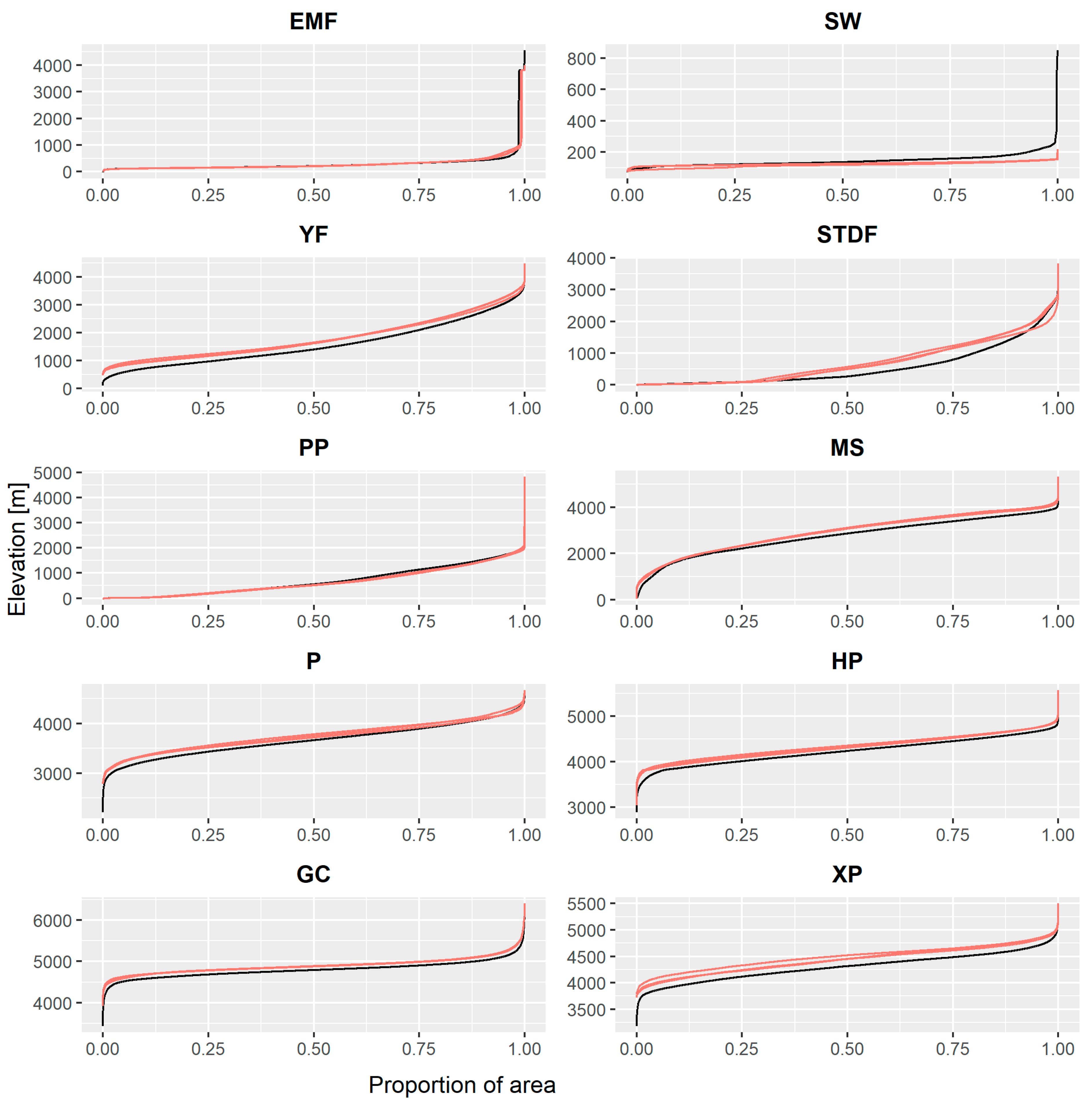
The percentage relationship of accumulated area is plotted versus elevation, that is, the hypsometric curve of each B. This representation was performed together for the present distribution and the projected future distributions. The graph allowed us to evaluate the vertical displacements of the elevations and the occupied areas for the B towards the period 2035–2065.

2.6.3. Regions Most Susceptible to Changes in Biomes

To estimate the susceptibility of the biomes, the agreement between the 3 RCMs for future projections was taken into account. Basically, we evaluated the changes in vertical structures based on the movements between the physiognomies and the changes in moisture levels associated with each biome; see Table 1. The categories of agreement for this document were adapted from Tovar et al. [18] and were the following: (1) increase in vertical structure, (2) increase in vertical structure and moisture, (3) increase in moisture and stable plant physiognomy, (4) no change, (5) decrease in moisture and stable physiognomy, (6) decrease in vertical structure and moisture, and (7) decrease in vertical structure. For the result of the agreement to be located in any of the aforementioned categories, it was necessary that at least 2 of the 3 models coincide. Otherwise, it was classified as an eighth category, divergence.

3. Results

3.1. Selection of the Biome Classification Model

Table 2. Efficiency indicators of the cross-validations for each bioclimatic model using the training data (80% of the current map).

K-Fold	Precision	Recall	F1 Score
	RF	RF	RF
1	0.805	0.897	0.842
2	0.802	0.894	0.839
3	0.803	0.894	0.840
4	0.804	0.898	0.842
5	0.802	0.895	0.839
Mean	0.803	0.896	0.841
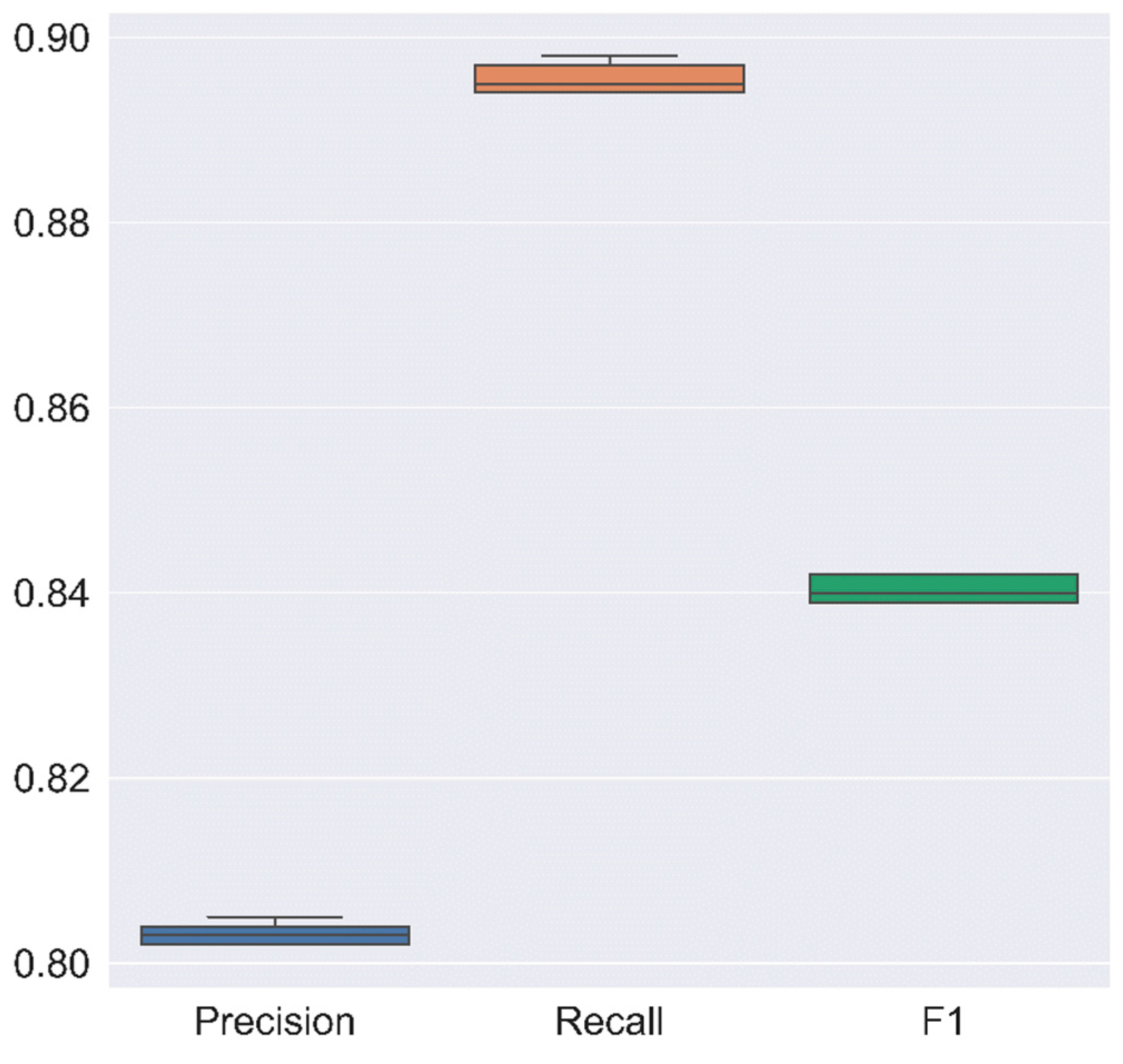
Standard deviation	0.001	0.002	0.001

was constructed with the training data (80% of the total data) and summarizes the efficiency indicators for RF while Figure A2 shows the dispersion in box plots. RF presents consistency in the cross-validations since its uncertainty is reduced (small standard deviation) with an average value in each fold of approximately 0.80.

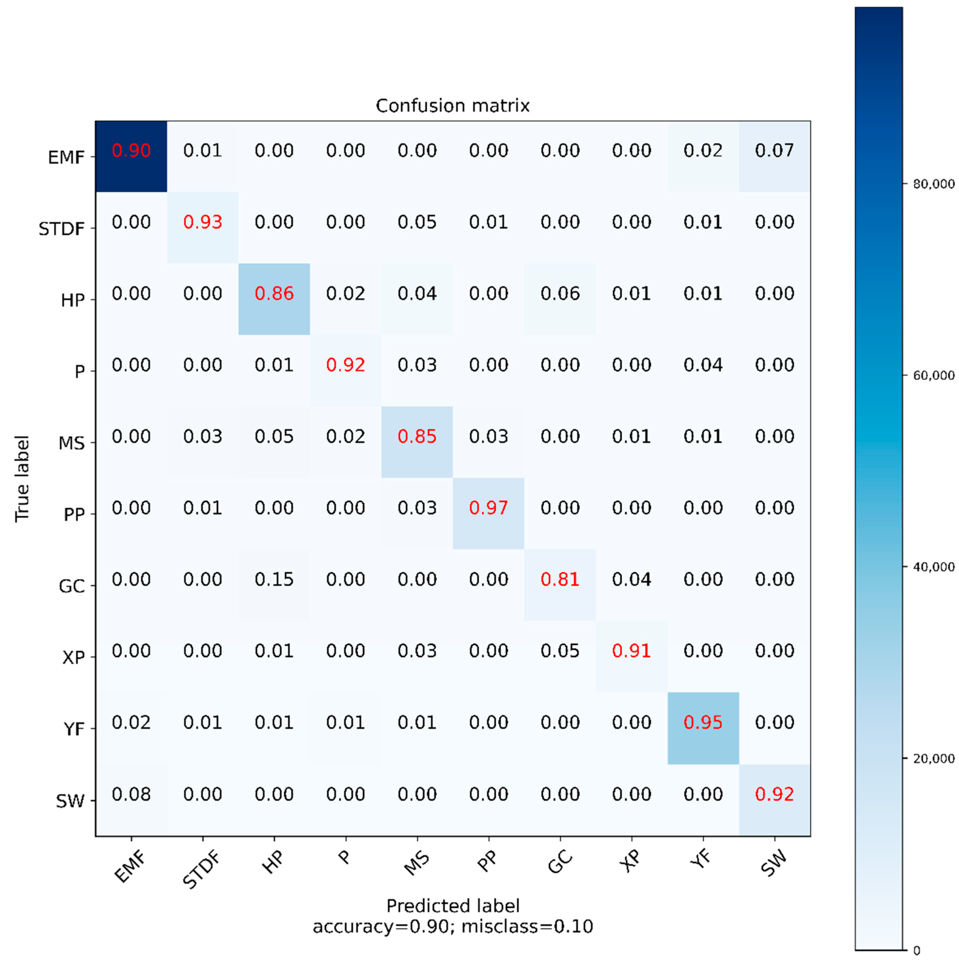
The RF confusion matrix (

Table 3. Confusion matrix of biomes with RF (pixels) constructed with the test data (20% of the observed map). The rows represent the biomes of the present map, while the columns represent the biomes classified by RF. The number of correctly classified pixels is displayed on the diagonals.

	EMF	SDTF	HP	P	MS	PP	GC	XP	YF	SW	Recall
EMF	98432	700	287	96	269	98	71	26	2155	7568	0.90
SDTF	16	5819	0	0	319	80	0	0	44	0	0.93
HP	13	1	28851	725	1217	0	2017	226	351	0	0.86
P	0	0	29	2521	69	0	5	0	105	0	0.92
MS	1	556	1127	450	17792	545	15	244	230	0	0.85
PP	7	113	0	0	389	14776	0	0	0	0	0.97
GC	0	0	879	23	6	0	4744	231	0	0	0.81
XP	0	0	34	0	69	0	116	2275	0	0	0.91
YF	526	181	349	505	275	0	0	0	33226	2	0.95
SW	980	0	0	0	0	0	0	0	2	11591	0.92
Precision	0.98	0.79	0.91	0.58	0.87	0.95	0.68	0.76	0.92	0.60

), indicates that the model in general has a completeness above 0.80. This means that the model is sensitive for detecting biomes. However, this high sensitivity was compensated with a lower precision since the model significantly overestimated some biomes, such as P, SW, and GC. HP and MS were erroneously classified as P in some cases, EMF as SW, and HP as GC. However, these classification statistics by RF are acceptable and show results superior to those of Tovar et al. [18].

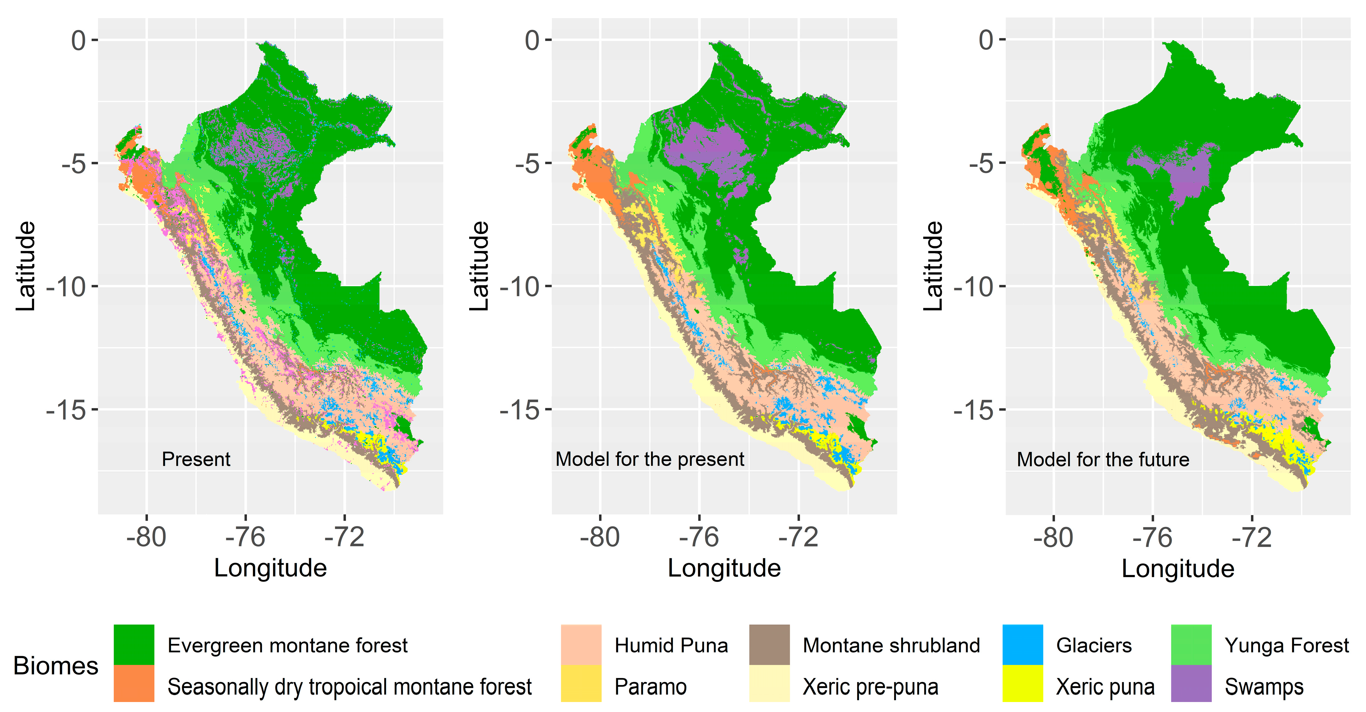
The spatial patterns of the present configuration of B performed with RF can be visualized in Figure 3. We can see a slight overestimation of the biomes: SW, P, and GC as described in the previous paragraph.

3.2. Vertical Displacements

Almost all B showed a vertical displacement in elevation, especially in their upper limit, except for SW, which receded at lower altitudes (see Figure 4). The SDTF biome significantly raised its average altitudes compared to the others. The YF in turn presented a vertical displacement of its lower boundary. The three RCMs showed agreement in the elevation changes.

3.3. Extension Changes in Biomes

The changes in the distribution of B areas were evaluated for the present (1981–2015) and future (2035–2065) periods using the median of the 3 RCMs. Figure 4 shows the migration of a present B to others in the future based on climate change scenarios in percentage values, while

Table A2. Migration matrix and biomes extension gains in km². The results are the median of the three regional climate models projections.

	EMF	SDTF	HP	P	MS	PP	GC	XP	YF	SW
EMF	506.69	0.59	1.27	0.02	0.93	0.25	0	0.04	1.26	14.85
SDTF	13.44	31	0	0	1.33	0.65	0	0	0.18	0
HP	0.07	0	133.67	3.31	21.29	0	1.26	2.03	2.89	0
P	0	0	2.05	15.74	5.34	0	0.01	0	2.53	0
MS	0.07	5.91	1.07	0.66	116.55	2.05	0	0.06	3.31	0
PP	0.74	6.95	0	0	8.91	74.5	0	0	0	0
GC	0	0	15.24	0.12	0.03	0	16.31	4.57	0	0
XP	0	0	1.77	0	2.49	0.01	0.09	10.07	0	0
YF	30.35	1.46	0.08	0.16	1.58	0	0	0	151.61	0
SW	68.73	0	0	0	0	0	0	0	0	30.61

are absolute values in thousands of km². The diagonal indicates the stable percentage of the ten B. The sum per row in Figure 4 is the current 100% coverage distributed in the future biomes, while the sum of the columns in Table A2 indicates the total area (km²) in the future for each biome.

The configurations of the B in the future project that 82% of the current distribution would remain stable; these results are similar to those of Tovar et al. [18]. The B that conserves almost the entirety of its present area is EMF, maintaining 96.4% having migrated in reduced quantities, and 2.83% towards the SW biome. Meanwhile, the B with the greatest losses was SW, which only maintained 30.8% of its present area. The second B with the highest losses was the CG, which changed towards HP by 42%. The relatively stable B were MS, PP, and YF, which conserved 89.82%, 81.79%, and 81.85% of their current area, respectively.

3.4. Regions Most Susceptible to Changes in Their Biomes

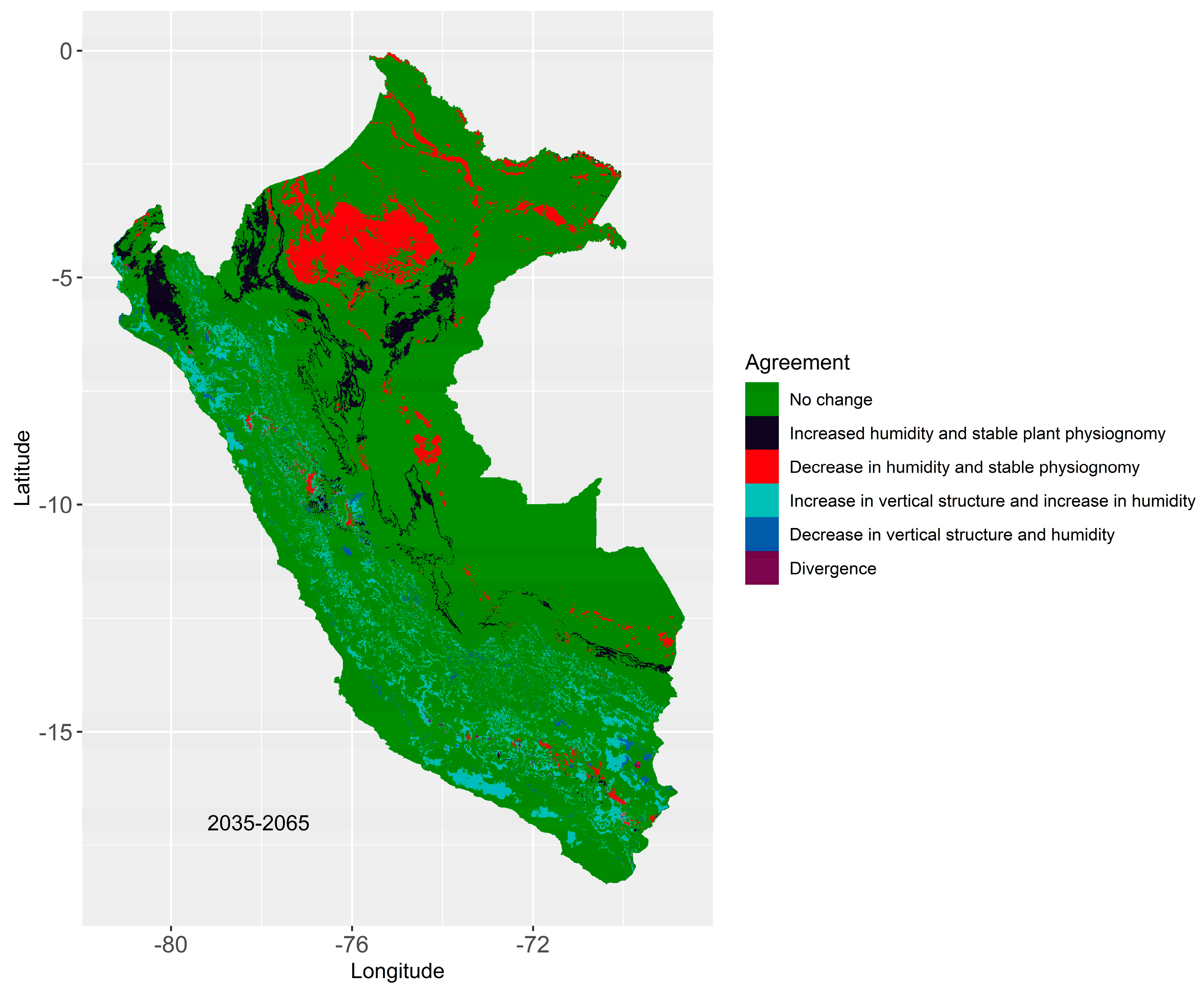
In Figure 5, it is observed that comparing the 3 RCMs for 2035–2065, the B specialization maintained stable 83% (agreement) of the currently occupied B area distributions. The approximate changing area represented 17%, while the area in disagreement (divergence) was 0.12%, which was a very small amount. Furthermore, the changed area was divided as follows: Increase in moisture and stable plant physiognomy (4.47%), decrease in moisture and stable physiognomy (5.88%), and finally an increase in vertical structure and moisture (5.87%).

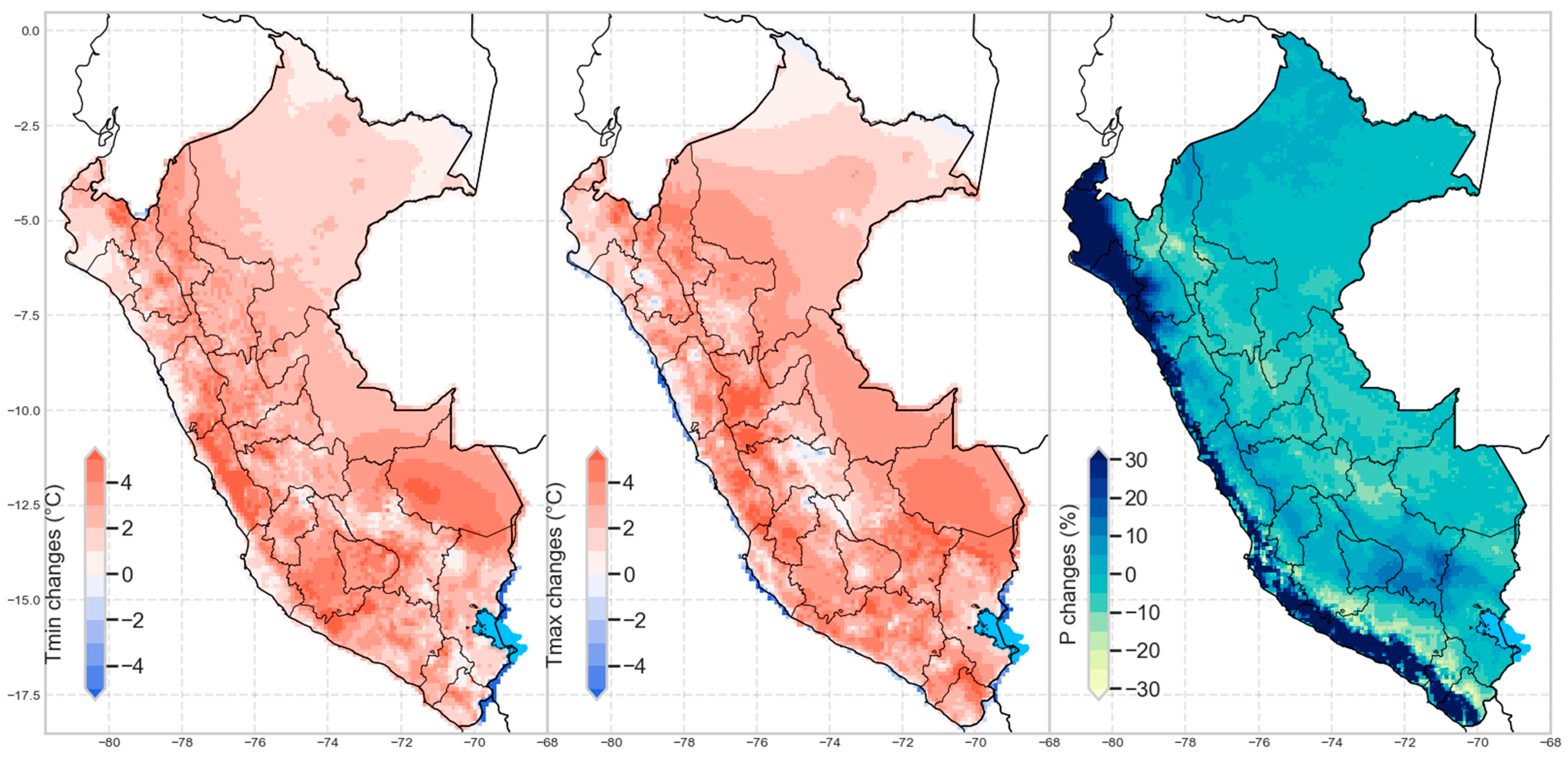
The areas of greatest change were in the northern part of the country, with Loreto and Piura being the departments with the greatest agreement towards a change in their B (Figure 5). We can observe a considerable decrease in humidity in the north of the Amazon due to temperature increases in the area (see Figure A1). Likewise, this area presented a high migration from SW to EMF.

The increase in humidity and stable physiognomy was distributed between the northern coast and the Peruvian forest, while the increase in vertical structure (4.47%) and humidity (5.87%) was distributed along the Andes with a greater spatial dispersion, see

Table 4. Biome migration matrix from the present (1981–2010) to the future (2035–2065) in percentage using the median of the 3 RCMs. The results in parentheses show the relative extent min–max of biomes that migrate.

	EMF	SDTF	HP	P	MS	PP	GC	XP	YF	SW
EMF	96.4 (95.7–98.4)	0.11	0.24	0	0.18	0.05	0	0.01	0.24	2.83 (0.6–3.5)
SDTF	28.85 (24.6–32.6)	66.55 (60.8–70.7)	0	0	2.86 (1.9–5.5)	1.4 (0.8–1.9)	0	0	0.39	0
HP	0.04	0	78.35 (75.5–86.7)	1.94 (0.7–4.9)	12.48 (9.1–17.1)	0	0.74 (0.3–1.0)	1.19 (0.7–4.7)	1.69 (0.5–1.7)	0
P	0	0	7.82 (5.9–9.6)	60.01 (59.9–62.1)	20.36 (20.2–25.2)	0	0.03	0	9.65 (8.7–10.0)	0
MS	0.05	4.56 (4.2–4.9)	0.82	0.51	89.82 (89.2–89.9)	1.58	0	0.05	2.55 (1.2–3.3)	0
PP	0.81	7.62 (4.2–10.8)	0	0	9.78 (8.6–11.9)	81.79 (76.2–86.9)	0	0	0	0
GC	0	0	41.99 (39.4–44.4)	0.34	0.09	0	44.95 (43.3–45.1)	12.58	0	0
XP	0	0	11.65 (0.5–16.1)	0	16.41 (11.5–21.2)	0.06	0.59 (0.5–1.3)	66.34 (66–87.3)	0	0
YF	16.38 (14.8–22.92)	0.79 (0.7–1.5)	0.04	0.09	0.85 (0.7–4.1)	0	0	0	81.85 (70.9–83.6)	0
SW	69.19 (56.6–94.2)	0	0	0	0	0	0	0	0	30.81 (5.7–43.3)

and Figure 5. These areas projected migration towards EMF for the former and MS-SDTF for the latter.

4. Discussion

The methodology developed has allowed us to appreciate the possible effects caused by climate change in the B in Peru, evaluating the consistency of three future climate projections based on regional climate models. However, as in any projection model, the methodological uncertainties related to the climate models and the present B modeling process must be mentioned to be considered in the conversation plans and decision-making in the face of climate change. In the following sections, we discuss the weaknesses and strengths of our results, as well as the results obtained for the 2035–2065 horizon.

4.1. Changes in Biomes

Our results show that the montane shrubland and xeric puna have an increase in area under the effects of climate change. As these B are located at medium elevations, they can move to higher altitudes to find their equilibrium and therefore have a better adaptation. In contrast, B with higher humidity suffer contraction and losses of areas mainly in sectors with lower elevations. These displacements have also been observed in other studies [5,18]. This pattern of elevation displacement can be explained by the water balance since, when there is an increase in temperature (shown in our projections), the availability of water can be reduced by increasing evapotranspiration.

It is worth mentioning that the displacement of B could force farmers to move to higher altitudes and increase the cultivation areas. This process can lead to greater difficulty in the adaptation of biomes during their migration. For example, Ovalle Rivera et al. [41] mention that increases in temperature could increase deforestation to develop coffee crops. These human interventions limit the development of potential areas of emerging biomes. In Peru, there are agricultural areas between 3000–3500 amsl that hinder the migration of forests to higher areas [42].

Although our study only considered changes due to climate change at the B level, the species that inhabit them could be affected by the threat of extinction or displacement to higher elevations [43,44]. These migrations can create competition between migrant and existing species. In addition, new climatic conditions can increase the difficulty of adaptation since they would be developing in less time compared to the last ice age [45,46,47].

4.2. Most Susceptible Biomes and Projected Changes

The B with the greatest risk to be reduced are glaciers and swamps. The projected losses for both are greater than 50% of their present area. For the former, the difficulty of not being able to move to higher altitudes with lower temperatures is one of the main causes of their losses. The latter, having drier conditions due to temperature increases, undergoes a process of change of vegetation from palm trees to wood trees, since they support conditions with lower humidity.

The estimated areas of discrepancy were reduced, which may be due to the use of only 3 RCMs compared to other studies [16,48]. Additionally, it is observed that there is a direct relationship between the vertical displacements and the humidity levels; that is, an increase in the humidity level implies an increase in the vertical structure, while a decrease in humidity generates a decrease in the vertical structure. Tovar et al. [18] argue that these vertical reductions affect carbon storage.

In contrast, our results show that the evergreen montane forest and seasonally dry tropical montane forest are quite stable, consistent with what has been observed in the past 30 thousand years [12]. However, only the evergreen montane forest will increase its area with area migrations to where the swamps are in the present.

4.3. Analysis of the Modeling of Biomes

The modeling of the present B with RF manages to represent the existing complexity in the climatic limits of each B [36,49]. One way to improve the model is by using the assemblies of various machine learning models, as presented by Bax et al. [19]. However, RF is itself an assembly model of several decision trees, which is why it has a higher performance compared to other classification algorithms.

Additionally, the reduced dispersion of the efficiency indicators shown by RF in the cross-validations indicates consistency on the part of the model to perform simulations with data that have not been used in its calibration. However, the interpretability of the model is complicated. Even so, the independent sensitivity of RF for the detection of B is high compared to the results obtained by Tovar et al. [18]. This sensitivity to classify biomes in this study benefits the determination of B with less national coverage, such as glaciers.

Another of the difficulties present in the research is the small number of climate models used in the evaluation of the changes in B. The uncertainty associated with future climate projections is not properly quantified. However, agreement was observed in the RCMs used. Additionally, some studies make future projections for more horizons so that they can be identified when a conservation policy can intervene [17]. Despite this, the identification of vulnerable areas demarcated in this study allows decision-makers to focus adaptation plans for economies dependent on ecosystem services at risk [50,51].

It should be noted that the comparison of trends and results between the different studies is difficult since the initial delineation of the boundaries of the Bs varies from study to study. This variation can be explained by current remote sensing tools that allow us to focus on macroscopic characteristics ignoring plant characteristics and focus more on the phenology and functional types of plants, so there is subjectivity when delimiting the B limits [52]. In addition, the grouping of biomes can be arbitrarily biased to reach a high efficiency in the performance indicators, which denatures ecological characteristics and transforms the problem to a purely numerical optimization approach.

Finally, our model does not consider land uses in the estimates. This omission may have led to more optimistic results than those that could be presented in the future. For example, an increase in agricultural areas or tree felling has been observed, whose impact is not estimated in our modeling [53]. The change in land use affects the dynamics of the ecosystem and the control of natural flow, so there is a need to balance the short-term ecosystem benefits and the long-term future climate costs associated with conservation plans [54]. A future update of the results should consider changes in land use and an expansion of the number of climate change models. A better understanding of ecological relationships could improve the selection of predictor variables and provide a better approximation of the present and future situation.

5. Conclusions

In this study, the map of present biomes at a spatial resolution of 1 km were estimated using the random forest model with in situ data for Peru. It was possible to prove not only the efficiency of the random forest for the classification of biomes for its prediction stability but also the predictive capacity of the bioclimatic variables despite the complex climatic variability present in Peru.

Regarding the impact of climate change on the distribution of biomes, based on 3 regional climate change models, our results are similar to other studies since a stable area of 83% of all present biomes, which were in our vertical displacement projections, was estimated. Additionally, it was possible to identify that the most susceptible biomes with losses greater than 50% of their present area were swamps and glaciers. These susceptible areas would be under water stress, which would cause a migration of species and changes in their physiognomy. It should be noted that these projections do not consider land use, even though in recent years and in future projections, they project large changes in the land use of important areas.

Future work should focus on improving the delimitation of current biomes as ecological knowledge advances. In addition, on improving the classification models with better data quality and the inclusion of human activity, such as land use. Despite our simplifications in this study, a consistent analysis on the biomes in Peru is provided for decision-makers and the scientific community.

References

- Cramer, W.; Bondeau, A.; Woodward, F.I.; Prentice, I.C.; Betts, R.A.; Brovkin, V.; Cox, P.M.; Fisher, V.; Foley, J.A.; Friend, A.D.; et al. Global response of terrestrial ecosystem structure and function to CO2 and climate change: Results from six dynamic global vegetation models. Glob. Chang. Biol. 2001, 7, 357–373. [Google Scholar] [CrossRef] [Green Version]
- Moncrieff, G.R.; Bond, W.J.; Higgins, S.I. Revising the biome concept for understanding and predicting global change impacts. J. Biogeogr. 2016, 863–873. [Google Scholar] [CrossRef]
- Olson, D.M.; Dinerstein, E.; Wikramanayake, E.D.; Burgess, N.D.; George, V.N.; Underwood, E.C.; Jennifer, A.D.; Itoua, I.; Strand, H.E.; Morrison, J.C.; et al. Terrestrial Ecoregions of the World: A New Map of Life on Earth. BioScience 2001, 51, 933–938. [Google Scholar] [CrossRef]
- Prentice, I.C.; Sykes, M.T.; Cramer, W. The possible dynamic response of northern forests to global warming. Glob. Ecol. Biogeogr. Lett. 1991, 1, 129–135. [Google Scholar] [CrossRef] [Green Version]
- Chakraborty, A.; Joshi, P.K.; Ghosh, A.; Areendran, G. Assessing biome boundary shifts under climate change scenarios in India. Ecol. Indic. 2013, 34, 536–547. [Google Scholar] [CrossRef]
- Holdridge, L.R. Determination of World Plant Formations From Simple Climatic Data. Science 1947, 105, 367–368. [Google Scholar] [CrossRef]
- Walter, H.; Richards, P.W.; Wieser, J. Vegetation of the Earth in Relation to Climate and the Eco-Physiological Conditions. J. Ecol. 1973, 63, 1014–1015. [Google Scholar] [CrossRef]
- Lopes, M.S.; Veettil, B.K.; Saldanha, D.L. Buffer zone delimitation of conservation units based on map algebra and AHP technique: A study from Atlantic Forest Biome (Brazil). Biol. Conserv. 2021, 253, 108905. [Google Scholar] [CrossRef]
- Gallego-Sala, A.V.; Colin Prentice, I. Blanket peat biome endangered by climate change. Nat. Clim. Chang. 2013, 3, 152–155. [Google Scholar] [CrossRef]
- Rasquinha, D.N.; Sankaran, M. Modelling biome shifts in the Indian subcontinent under scenarios of future climate change. Curr. Sci. 2016, 111, 147–156. [Google Scholar] [CrossRef]
- Heubes, J.; Kühn, I.; König, K.; Wittig, R.; Zizka, G.; Hahn, K. Modelling biome shifts and tree cover change for 2050 in West Africa. J. Biogeogr. 2011, 38, 2248–2258. [Google Scholar] [CrossRef]
- Costa, G.C.; Hampe, A.; Pablo, M.L.; Mazzochini, G.G.; Shepard, D.B.; Werneck, F.P.; Moritz, C.; Carolina, A. Biome stability in South America over the last 30 kyr: Inferences from long-term vegetation dynamics and habitat modelling. Glob. Ecol. Biogeogr. 2018, 27, 285–297. [Google Scholar] [CrossRef]
- Giudicelli, G.C.; Turchetto, C.; Silva-Arias, G.A.; Freitas, L.B. Influence of climate changes on the potential distribution of a widespread grassland species in South America. Perspect. Plant Ecol. Evol. Syst. 2019, 41, 125496. [Google Scholar] [CrossRef]
- MINAM (Ministerio del Ambiente). Mapa Nacional de Ecosistemas del Perú—Memoria Descriptiva. 2019. Available online: https://redd.unfccc.int/files/nref_peru_final.pdf (accessed on 30 September 2021).
- Scullion, J.J.; Vogt, K.A.; Sienkiewicz, A.; Gmur, S.J.; Trujillo, C. Assessing the influence of land-cover change and conflicting land-use authorizations on ecosystem conversion on the forest frontier of Madre de Dios, Peru. Biol. Conserv. 2014, 171, 247–258. [Google Scholar] [CrossRef]
- Brêda, J.P.L.F.; de Paiva, R.C.D.; Collischon, W.; Bravo, J.M.; Siqueira, V.A.; Steinke, E.B. Climate change impacts on South American water balance from a continental-scale hydrological model driven by CMIP5 projections. Clim. Chang. 2020, 159, 503–522. [Google Scholar] [CrossRef]
- Boit, A.; Sakschewski, B.; Boysen, L.; Cano-Crespo, A.; Clement, J.; Garcia-alaniz, N.; Kok, K.; Kolb, M.; Langerwisch, F.; Rammig, A.; et al. Large-scale impact of climate change vs. land-use change on future biome shifts in Latin America. Glob. Chang. Biol. 2016, 22, 3689–3701. [Google Scholar] [CrossRef]
- Tovar, C.; Arnillas, C.A.; Cuesta, F.; Buytaert, W. Diverging Responses of Tropical Andean Biomes under Future Climate Conditions. PLoS ONE 2013, 8, e63634. [Google Scholar] [CrossRef] [Green Version]
- Bax, V.; Castro-Nunez, A.; Francesconi, W. Assessment of potential climate change impacts on montane forests in the peruvian andes: Implications for conservation prioritization. Forests 2021, 12, 375. [Google Scholar] [CrossRef]
- Ramirez-Villegas, J.; Cuesta, F.; Devenish, C.; Peralvo, M.; Jarvis, A.; Arnillas, C.A. Using species distributions models for designing conservation strategies of Tropical Andean biodiversity under climate change. J. Nat. Conserv. 2014, 22, 391–404. [Google Scholar] [CrossRef] [Green Version]
- Garreaud, R.D.; Vuille, M.; Compagnucci, R.; Marengo, J. Present-day South American climate. Palaeogeogr. Palaeoclimatol. Palaeoecol. 2009, 281, 180–195. [Google Scholar] [CrossRef]
- Lavado Casimiro, W.S.; Ronchail, J.; Labat, D.; Espinoza, J.C.; Guyot, J.L. Basin-scale analysis of rainfall and runoff in Peru (1969–2004): Pacific, Titicaca and Amazonas drainages. Hydrol. Sci. J. 2012, 57, 625–642. [Google Scholar] [CrossRef] [Green Version]
- Castro, A.; Davila, C.; Laura, W.; Cubas, F.; Ávalos, G.; Ocaña, C.L.; Villena, D.; Valdez, M.; Urbiola, J.; Trebejo, I.; et al. Climas del Perú. In Mapa de Clasificación Climática Nacional; 2020; Available online: https://www.senamhi.gob.pe/load/file/01404SENA-4.pdf (accessed on 30 September 2021).
- Funk, C.; Peterson, P.; Landsfeld, M.; Pedreros, D.; Verdin, J.; Shukla, S.; Husak, G.; Rowland, J.; Harrison, L.; Hoell, A.; et al. The climate hazards infrared precipitation with stations—A new environmental record for monitoring extremes. Sci. Data 2015, 2, 150066. [Google Scholar] [CrossRef] [Green Version]
- Vancutsem, C.; Ceccato, P.; Dinku, T.; Connor, S.J. Evaluation of MODIS land surface temperature data to estimate air temperature in different ecosystems over Africa. Remote Sens. Environ. 2010, 114, 449–465. [Google Scholar] [CrossRef]
- Aybar, C.; Fernández, C.; Huerta, A.; Lavado, W.; Vega, F. Construction of a high-resolution gridded rainfall dataset for Peru from 1981 to the present day. Hydrol. Sci. J. 2020, 65, 770–785. [Google Scholar] [CrossRef]
- Fick, S.E.; Hijmans, R.J. WorldClim 2: New 1-km spatial resolution climate surfaces for global land areas. Int. J. Climatol. 2017, 37, 4302–4315. [Google Scholar] [CrossRef]
- Hijmans, R.J.; Elith, J. Species distribution modeling with R Introduction. R CRAN Proj. 2013, 6, 71. [Google Scholar]
- Skamarock, W.C.; Klemp, J.B.; Dudhia, J.B.; Gill, D.O.; Barker, D.M.; Duda, M.G.; Huang, X.-Y.; Wang, W.; Powers, J.G. A description of the Advanced Research WRF Version 3, NCAR Technical Note TN-475+STR. Tech. Rep. 2008. [Google Scholar] [CrossRef]
- Jungclaus, J.H.; Fischer, N.; Haak, H.; Lohmann, K.; Marotzke, J.; Matei, D.; Mikolajewicz, U.; Notz, D.; Von Storch, J.S. Characteristics of the ocean simulations in the Max Planck Institute Ocean Model (MPIOM) the ocean component of the MPI-Earth system model. J. Adv. Model. Earth Syst. 2013, 5, 422–446. [Google Scholar] [CrossRef]
- Bi, D.; Dix, M.; Marsland, S.J.; O’Farrell, S.; Rashid, H.A.; Uotila, P.; Hirst, A.C.; Kowalczyk, E.; Golebiewski, M.; Sullivan, A.; et al. The ACCESS coupled model: Description, control climate and evaluation. Aust. Meteorol. Oceanogr. J. 2013, 63, 41–64. [Google Scholar] [CrossRef]
- Collins, W.J.; Bellouin, N.; Doutriaux-Boucher, M.; Gedney, N.; Halloran, P.; Hinton, T.; Hughes, J.; Jones, C.D.; Joshi, M.; Liddicoat, S.; et al. Development and evaluation of an Earth-System model—HadGEM2. Geosci. Model Dev. 2011, 4, 1051–1075. [Google Scholar] [CrossRef] [Green Version]
- Luo, M.; Liu, T.; Meng, F.; Duan, Y.; Frankl, A.; Bao, A.; De Maeyer, P. Comparing bias correction methods used in downscaling precipitation and temperature from regional climate models: A case study from the Kaidu River Basin in Western China. Water 2018, 10, 1046. [Google Scholar] [CrossRef] [Green Version]
- Blaustein, A.R. Predicting climate-induced range shifts: Model differences and model reliability. Glob. Chang. Biol. 2006, 12, 1568–1584. [Google Scholar] [CrossRef] [Green Version]
- Breiman, L.E.O. Random Forests. Mach. Learn. 2001, 45, 5–32. [Google Scholar] [CrossRef] [Green Version]
- Cutler, D.R.; Edwards, T.C.; Beard, K.H.; Cutler, A.; Hess, K.T.; Gibson, J.; Lawler, J.J. Random forests for classification in ecology. Ecology 2007, 88, 2783–2792. [Google Scholar] [CrossRef]
- Duchesnay, F.P.; Varoquaux, G.; Gramfort, A.; Michel, V.; Thirion, B.; Grisel, O.; Blondel, M.; Prettenhofer, P.; Weiss, R.; Dubourg, V.; et al. Scikit-learn: Machine Learning in Python. J. Mach. Learn. Res. 2011, 12, 2825–2830. [Google Scholar]
- Maraun, D.; Widmann, M. Statistical Downscaling and Bias Correction for Climate Research. Stat. Downscal. Bias Correct. Clim. Res. 2018. [Google Scholar] [CrossRef] [Green Version]
- Gutiérrez, J.M.; Maraun, D.; Widmann, M.; Huth, R.; Hertig, E.; Benestad, R.; Roessler, O.; Wibig, J.; Wilcke, R.; Kotlarski, S.; et al. An intercomparison of a large ensemble of statistical downscaling methods over Europe: Results from the VALUE perfect predictor cross-validation experiment. Int. J. Climatol. 2019, 39, 3750–3785. [Google Scholar] [CrossRef]
- Chen, J.; Brissette, F.P.; Leconte, R. Coupling statistical and dynamical methods for spatial downscaling of precipitation. Clim. Chang. 2012, 114, 509–526. [Google Scholar] [CrossRef]
- Ovalle-Rivera, O.; Läderach, P.; Bunn, C.; Obersteiner, M.; Schroth, G. Projected shifts in Coffea arabica suitability among major global producing regions due to climate change. PLoS ONE 2015, 10, e0124155. [Google Scholar] [CrossRef] [Green Version]
- Rehm, E.M.; Feeley, K.J. The inability of tropical cloud forest species to invade grasslands above treeline during climate change: Potential explanations and consequences. Ecography 2015, 38, 1167–1175. [Google Scholar] [CrossRef] [Green Version]
- Sekercioglu, C.H.; Schneider, S.H.; Fay, J.P.; Loarie, S.R. Climate change, elevational range shifts, and bird extinctions. Conserv. Biol. 2008, 22, 140–150. [Google Scholar] [CrossRef] [PubMed]
- Feeley, K.J.; Silman, M.R. Land-use and climate change effects on population size and extinction risk of Andean plants. Glob. Chang. Biol. 2010, 16, 3215–3222. [Google Scholar] [CrossRef]
- Valencia, B.G.; Urrego, D.H.; Silman, M.R.; Bush, M.B. From ice age to modern: A record of landscape change in an Andean cloud forest. J. Biogeogr. 2010, 37, 1637–1647. [Google Scholar] [CrossRef]
- Bush, M.B.; Silman, M.R.; Urrego, D.H. 48,000 Years of Climate and Forest Change in a Biodiversity Hot Spot. Science 2004, 303, 827–829. [Google Scholar] [CrossRef] [PubMed] [Green Version]
- Malcolm, J.R.; Markham, A.; Neilson, R.P.; Garaci, M. Estimated migration rates under scenarios of global climate change. J. Biogeogr. 2002, 29, 835–849. [Google Scholar] [CrossRef] [Green Version]
- Buytaert, W.; Bievre, B. De Water for cities: The impact of climate change and demographic growth in the tropical Andes. Water Resour. Res. 2012, 48, 1–13. [Google Scholar] [CrossRef] [Green Version]
- Park, S.; Park, H.; Im, J.; Yoo, C.; Rhee, J.; Lee, B.; Kwon, C.G. Delineation of high resolution climate regions over the Korean Peninsula using machine learning approaches. PLoS ONE 2019, 14, e0223362. [Google Scholar] [CrossRef]
- Buytaert, W.; Cuesta-Camacho, F.; Tobón, C. Potential impacts of climate change on the environmental services of humid tropical alpine regions. Glob. Ecol. Biogeogr. 2011, 20, 19–33. [Google Scholar] [CrossRef]
- Balvanera, P.; Uriarte, M.; Almeida-Leñero, L.; Altesor, A.; DeClerck, F.; Gardner, T.; Hall, J.; Lara, A.; Laterra, P.; Peña-Claros, M.; et al. Ecosystem services research in Latin America: The state of the art. Ecosyst. Serv. 2012, 2, 56–70. [Google Scholar] [CrossRef]
- Woodward, F.I.; Lomas, M.R.; Kelly, C.K. Global climate and the distribution of plant biomes. Philos. Trans. R. Soc. B Biol. Sci. 2004, 359, 1465–1476. [Google Scholar] [CrossRef] [Green Version]
- Salazar, L.F.; Nobre, C.A.; Oyama, M.D. Climate change consequences on the biome distribution in tropical South America. Geophys. Res. Lett. 2007, 34, 2–7. [Google Scholar] [CrossRef] [Green Version]
- Foley, J.A.; Asner, G.P.; Costa, M.H.; Coe, M.T.; Defries, R.; Gibbs, H.K.; Howard, E.A.; Olson, S.; Patz, J.; Ramankutty, N.; et al. Amazonia revealed: Forest degradation and loss of ecosystem goods and services in the Amazon Basin. Front. Ecol. Environ. 2007, 5, 25–32. [Google Scholar] [CrossRef]
Figure 1.
Multi-year climatology (1981–2010) of left: minimum temperature (°C), center: maximum temperature (°C), and right: precipitation (mm).
Figure 2.
Workflow for the classification of biomes of Peru.
Figure 3.
Biome maps of the present based on the MINAM Ecosystem map, representation of the present B with the RF model, and the representation of B projected to 2035–2065 of the ACCES1 model.
Figure 4.
Hypsometric curves of the modeled biomes for their present (black line) and future configurations (red lines).
Figure 5.
Concordance of biome projections with RF using different climate models for 2035–2065.