Dynamics of the Burlan and Pomacochas Lakes Using SAR Data in GEE, Machine Learning Classifiers, and Regression Methods

Abstract

Amazonas is a mountain region in Peru with high cloud cover, so using optical data in the analysis of surface changes of water bodies (such as the Burlan and Pomacochas lakes in Peru) is difficult, on the other hand, SAR images are suitable for the extraction of water bodies and delineation of contours. Therefore, in this research, to determine the surface changes of Burlan and Pomacochas lakes, we used Sentinel-1 A/B products to analyse the dynamics from 2014 to 2020, in addition to evaluating the procedure we performed a photogrammetric flight and compared the shapes and geometric attributes from each lake. For this, in Google Earth Engine (GEE), we processed 517 SAR images for each lake using the following algorithms: a classification and regression tree (CART), Random Forest (RF) and support vector machine (SVM).) 2021-02-10, then; the same value was validated by comparing the area and perimeter values obtained from a photogrammetric flight, and the classification of a SAR image of the same date. During the first months of the year, there were slight increases in the area and perimeter of each lake, influenced by the increase in rainfall in the area. CART and Random Forest obtained better results for image classification, and for regression analysis, Support Vector Regression (SVR) and Random Forest Regression (RFR) were a better fit to the data (higher R²), for Burlan and Pomacochas lakes, respectively. The shape of the lakes obtained by classification was similar to that of the photogrammetric flight. For 2021-02-10, for Burlan Lake, all 3 classifiers had area values between 42.48 and 43.53, RFR 44.47 and RPAS 45.63 hectares. For Pomacohas Lake, the 3 classifiers had area values between 414.23 and 434.89, SVR 411.89 and RPAS 429.09 hectares. Ultimately, we seek to provide a rapid methodology to classify SAR images into two categories and thus obtain the shape of water bodies and analyze their changes over short periods. A methodological scheme is also provided to perform a regression analysis in GC using five methods that can be replicated in different thematic areas.

1. Introduction

Only 2.5% of the planet’s water is fresh, of which only 1.2% is surface water, and much of the latter is found in glaciers and 20.9% is found in lakes [1]. There are more than 1.43 million lakes and reservoirs [2,3]. This type of coastal and continental ecosystem is important, being a source of nutritional resources for animals and humans, in addition to providing various ecosystem services [4].

Surface water resources also play important roles in economic development, the balance of terrestrial and aquatic ecosystems, agriculture, and the environment [5]. Therefore, it is crucial to monitor the dynamics of the area and water storage of a lake to evaluate the impacts of climate change and to predict future scenarios [6]. In addition, monitoring the extension of surface water supports the management of water resources and climate modelling, among other functions [7].

Detecting bodies of water near urban centres is also necessary for the delimitation of flood zones and therefore water accumulation, which become possible sources of outbreaks of water-borne diseases [8].

In recent years, with the increasing availability of free synthetic aperture radar (SAR) data, research on water resources has increased, for example, for the monitoring of the flooded surfaces of lakes in wet and dry seasons, especially small lakes [9], surface water quality monitoring [10], humidity mapping [11], river mapping [12], and the analysis of the spatiotemporal variation in the water surface of lakes [13].

In Jiangxi (China), the changes in the area of the water surface of Poyan Lake were analysed during 2014–2016 using 33 SAR images of Sentinel-1 and were processed in the Sentinel Application Platform (SNAP) [14]. In turn, Dongting Lake in China was monitored using SAR images from Environmental Satellite (Envisat) during 2002–2009 [15]. In Latin America, RADARSAT level 1 and 7 images, Japanese Earth Resources Satellite (JERS)-1 images, and aquatic vegetation were combined to calculate the area of the swamps of southern Brazil [16]. The lakes of northern Alaska were also mapped in the winter season of 2009 using European Remote Sensing satellite (ERS)-2 images to quantify the availability of water in winter and summer [17].

The classification of satellite images through classification and regression trees (CART), random forests (RF), and support vector machines (SVM) has achieved efficient and accurate results [18]. The image classification process mainly involves the assignment of pixels to a class based on spectral signatures, indices, contextual information, etc. [19]. For this, two known methods of joint learning are boosting and bagging [20]. In boosting, successive trees give extra weight to the points incorrectly predicted by previous predictors, and then a weighted vote is taken for the prediction [20,21]. In bagging, successive trees do not depend on previous trees, and each tree is constructed independently using an initial sample of the dataset. Then, a simple majority vote is carried out for the prediction [20,22]. These processes were optimized with the launch of Google Earth Engine (GEE), allowing the parallel processing of geospatial data at a global scale using the Google cloud [23,24].

Statistical models are a simplification of reality expressed in a mathematical language, so to achieve such simplification assumptions must be made, such is the case of this research that we simplify the behaviour model of the lakes based on different dates from 2014 to 2020. The regression tries to predict a quantity or an expected value, unlike classification which tries to predict a category or class [25]. The main regression algorithms include simple linear regression (SLR), polynomial regression (PR), random forest regression (RFR), support vector regression (SVR), and decision tree regression (DTR), which can be quickly executed in Google Colaboratory (GC).

We analysed the dynamics of the water surface of two lakes in the Amazonas region of Peru. For this, (i) we processed 517 Sentinel-1 images for the period 2014–2020, using the GEE platform, (ii) with the area and perimeter values of each lake we applied five regression methods executed in Google Collaboratory, (iii) we calculated area and perimeter by classifying a SAR image from 2021-02-10 and compared with the value predicted by the best regressor and (iv) finally we compared the values calculated in iii with a photogrammetric flight performed on the same date (2021-02-10). In effect, this research sought to show the dynamics of the water surfaces of two lakes approximately 50 km apart, with different climatic conditions, geographic, and socioeconomic conditions, relying on the continuity of SAR image data from Sentinel-1.

In contrast to other studies, we calculated the water mask by classifying SAR images in Google Earth Engine using Classification and Regression Trees, Random Forest and Support Vector Machine, and compared them with a high-resolution orthomosaic obtained by a Remote Pilot Aircraft System. We also show the flexibility of performing a regression analysis in Google Colaboratory using Simple Linear Regression, Polynomial Regression, Support Vector Regression, Decision Trees Regression and Random Forest Regression methods, and the same regression methods can be applied to different thematic areas.

2. Materials and Methods

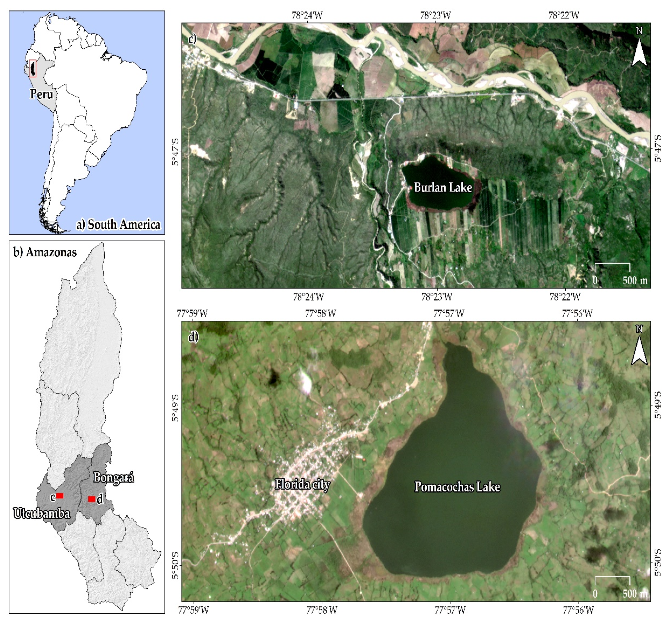
2.1. Study Area

Burlan and Pomacochas are two of the main lakes in the Amazonas region (NW Peru). Next, Figure 1 shows the geographic location of Burlan and Pomacochas Lake, in Utcubamba and Bongará provinces, respectively, in Amazonas region, Peru.

At Burlan Lake, the climate is warm, with an average temperature of 24.9 °C and an altitude of 450 m.a.s.l. [26]. Pomacochas Lake is in a warm and temperate climate, with an average annual temperature of 15 °C and an altitude of 2220 m.a.s.l. [27].

Both lakes have socioeconomic and environmental importance in terms of tourism, fishing and landscape services, water for agricultural activities, water resource regulation, and biodiversity.

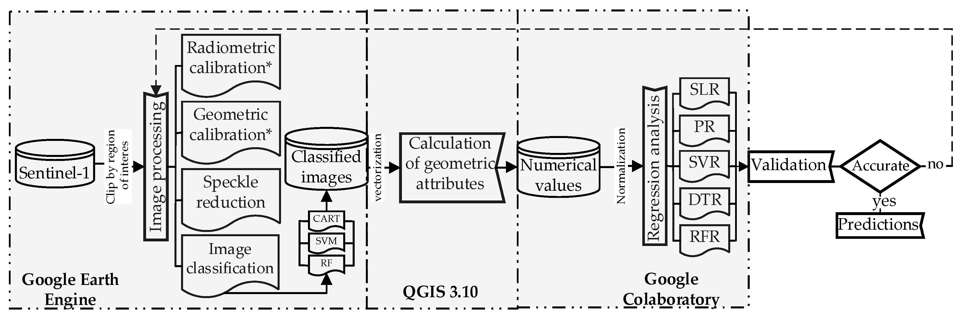
2.2. Methodological Scheme

Figure 2 summarizes the procedure for analyzing the water surface dynamics of the Burlan and Pomacochas lakes during 2014–2020 using images from the Sentinel-1 mission in GEE and five regression methods: SLR, PR, SVR, DTR and RFR. For this, initially, the speckle of the SAR images was reduced, for a subsequent classification using the CART, RF and SVM algorithms, the classified images were processed in QGIS 3.10. Subsequently, in Google Collaboratory through five regression methods and the area and perimeter values calculated in QGis, the area and perimeter were predicted for 2021-02-10, calculating the R² of each regression method. Finally, to validate the calculations performed in GEE and GC, the area and perimeter of each lake were measured in the field using a remotely piloted aircraft system (RPAS) for comparison to the area and perimeter obtained by the extraction in GEE and regression estimation of the method of greater R².

2.3. SAR Dataset and Training Points

Sentinel-1 A/B images (COPERNICUS/S1_GRD) available in GEE were used [28] with a temporal resolution of 6 days. The data used were level 1 in the ground range detection (GRD), interferometric wideband (IW) format (Beam Mode), with a 10 m resolution, using the ascending and descending Flight Direction, in addition, VH and VV cross-polarized scenes [29].

In the supervised classification of all SAR images, 23 and 12 training points were used for Pomacochas and Burlan Lakes, respectively. The points were categorized as water (1) and land (0), those labelled 1 were distributed in the center of the lake because the previous inspection of images is an area where water is always present, on the other hand, the points labelled 0 were distributed to the edges of the lakes, generally higher parts where there is no water concurrence. For more details on the training points, check file 09 of the web repository Available online: https://github.com/dargofer/SAR_image_classification (accessed on 15 October 2022).

2.4. SAR Image Processing

The processing of the SAR images was carried out in the GEE platform [23]. For this, a code was developed (check file 01 of the web repository), that included the import of Sentinel-1 images speckle reduction, classification, and export of SAR images. In addition, according to the availability of data and the objective of the research, water masks were generated in four combinations. For this, Flight Direction and the polarization of the images were combined. These combinations were Descending-VH (DVH), Ascending-VH (AVH), Descending-VV (DVV), and Ascending-VV (AVV) from 2014 to 2020.

For a correct analysis of the SAR images, they must be corrected radiometrically and geometrically, in addition, depending on the objective of the study, the speckle of the images is reduced [30]. In our case, we use the Sentinel-1 images available in the GEE data catalogue, as mentioned in the GEE processing guide for Sentinel-1 images. (Available online: https://developers.google.com/earth-engine/guides/sentinel1 (accessed on 15 January 2021)) these images were already radiometrically and geometrically corrected [29], so we only reduced the speckle of the images using ee.Image.focal_median [31].

A variable was created that contained the filtered collection and a band with the details of each of the four combinations. Then, we performed supervised classification with three machine learning algorithms [32], RF [33], CART [34], and SVM [35,36] algorithms, and 23 and 12 training points for Pomacochas and Burlan Lakes, respectively. Additionally, to evaluate the accuracy of the classification, we calculated the confusion matrix and kappa index [37]. Finally, the images classified in GeoTIFF format and the EPSG coordinate reference system were exported: 32,717 and 32,718 for Burlan and Pomacochas Lakes, respectively.

2.5. Calculation of the Geometric Attributes

The geometric attributes were calculated in the QGIS 3.10 LTR software, where the classified images were vectorized using the raster polygonize tool executed in batches. The classified images were dissolved according to their coding to avoid calculation errors because, in some images, separate polygons were generated with the same coding. Finally, the geometric values of the area and perimeter were added for each group of images.

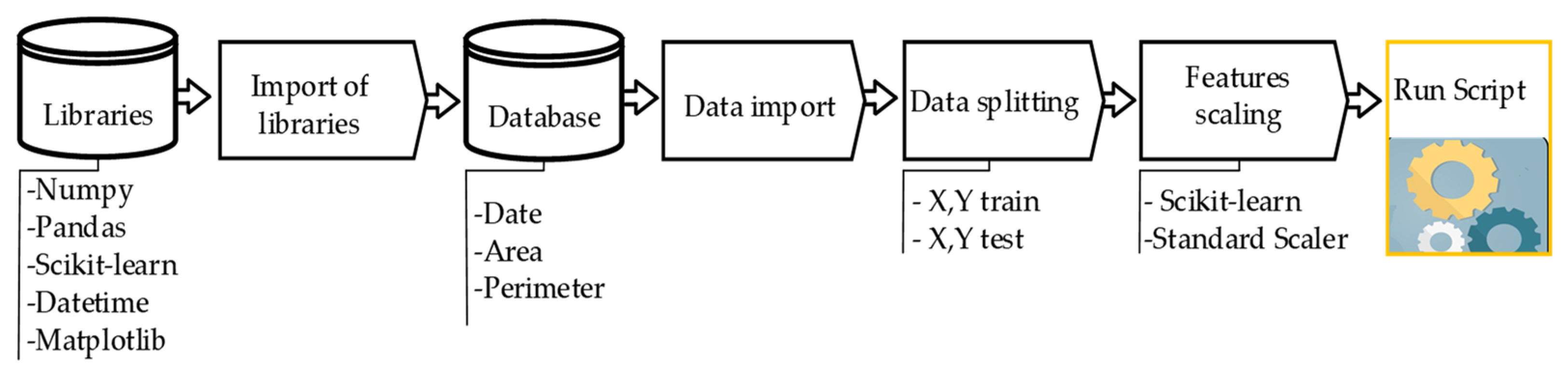
2.6. Regression Analysis

With the values obtained for the area and perimeter of each lake and each combination and classifier, five regression methods were applied to estimate the area value of a lake at a specific subsequent time. Simple Linear Regression, Polynomial Regression, Support Vector Regression, Decisions Trees Regression and Random Forest Regression were executed in scripts with Python coding language in Google Colaboratory.

Figure 3 shows the methodological flow chart used in the five regression methods, initially, the Python libraries were imported to input the database, in all 5 methods the database was split into training and evaluation, finally, a feature scaling and execution of the regression method script was performed.

The dependent variables were the area and perimeter (separately), and as an independent variable, the date of acquisition of the SAR image was transformed to an ordinal integer because, in the regressions, chains generate problems in the prediction. The main library used was Scikit-learn [38], which contains all the regression methods used in this research. Next, the procedure followed in each regression method is described.

For Simple Linear Regression, the Numpy, Pandas, Matplotlib, and Scikit-learn libraries were used. The fundamental equation of SLR was determined by the intercept (b₀), the slope (b₁), the independent variable (X) and the Random error term (e_i) (Equation (1)); since the goal of linear regression is to fit a straight line through the data that predicts Y based on X, the calculation of b₀ and b₁ is usually estimated by the ordinary least squares method (Equation (2)) [39,40]. The LinearRegression function was used as a regressor [41], imported from the linear models module of the Scikit-learn library.

Y_i = b₀ + b₁X_i + e_i

(1)

Σ (y_i − ŷ_i)²

(2)

To build the polynomial regression we mainly used the “PolynomialFeatures” function [42], which belongs to the scikit-learn library, for which, we used a simple linear regression equation, which was transformed to a second degree using the above-mentioned function.

For Support Vector Regression, the imported data were standardized using the Standard Scaler [43]. Then, to apply the principles of the theory of Vapnik Chervonenkis [44], in which at least the epsilon insensitive tube width and kernel function are required, the SVR function [45], from the Sklearn.svm module was imported. In addition, to complete the regressor, we used the Gaussian Radial Basis Function (RBF) as a kernel function for the Support Vector Regression [46], and 0.1 as the epsilon value.

To build the Random Forest Regression, we imported RandomForestRegressor [47], from the Sklearn.ensemble module and we considered the default number of trees (n_estimator = 10) and 0 as the state of randomness (random_state). Finally, to apply Decision Tree Regression to the data, DecisionTreeRegressor was imported [48] as a regressor from the Sklearn.tree module and the state of randomness was given the value of 0.

2.7. Field Data and Validation

The validation of the area and perimeter of each lake was carried out using images from photogrammetric flights performed on 2021-02-10 with a Phantom 4 RTK in post-processed kinematic mode (PPK) and ground control points (GCPs) collected with a Trimble R10 GNSS. For Pomacochas Lake, 2065 images with 4.57 cm average Ground Sampling Distance (GSD) were obtained, and for Burlan Lake, 729 images with 4.01 cm average GSD were obtained. All images were processed in PIX4D Mapper v 4.6.4 using 9 GCPs for each lake, then to uniformize the images, the orthomosaics were exported at resolutions of 50 cm/pixel.

The measurement of the tie point errors was performed by calculating the root mean square (RMS) error, because the RMS considers the mean error and the variance. Therefore, for a given direction (X, Y, or Z) the RMS is defined as:

$$\mathrm{RMS}=\sqrt{\mathsf{\Sigma } \frac{e_i{}^2}{N}}$$

(3)

where, ${\mathit{e}}_{\mathit{i}}$ is the error of each point for the given direction, and N is the number of GCPs.

Finally, for each lake, a SAR image from 2021-02-10 was classified and overlaid with the orthomosaics obtained by the RPAS.

On the other hand, the five regression methods were applied to each group with the area and perimeter data according to each classifier, from which the coefficient of determination (R²) available in Scikit-learn was calculated [49] to indicate the fit of the data. The R² values range from −∞ to 1, the best possible score is 1, and negative values refer to the model can be arbitrarily worse. Therefore, if ŷ_i is the predicted value of the i-th sample, and y_i is the corresponding true value for the total of n samples, the R² is defined as:

$${\mathrm{R}}^2 (y,\hat{y})=1-\frac{{\sum }_{i=1}^n{(y_i-{\hat{y}}_i)}^2}{{\sum }_{i=1}^n{(y_i-{\stackrel{-}{y}}_i)}^2} \mathrm{and} \stackrel{-}{y}=\frac{1}{n}{\sum }_{i=1}^n{y}_i, {\sum }_{i=1}^n{(y_i-{\hat{y}}_i)}^2={\sum }_{i=1}^n{ϵ}_i^2$$

(4)

3. Results

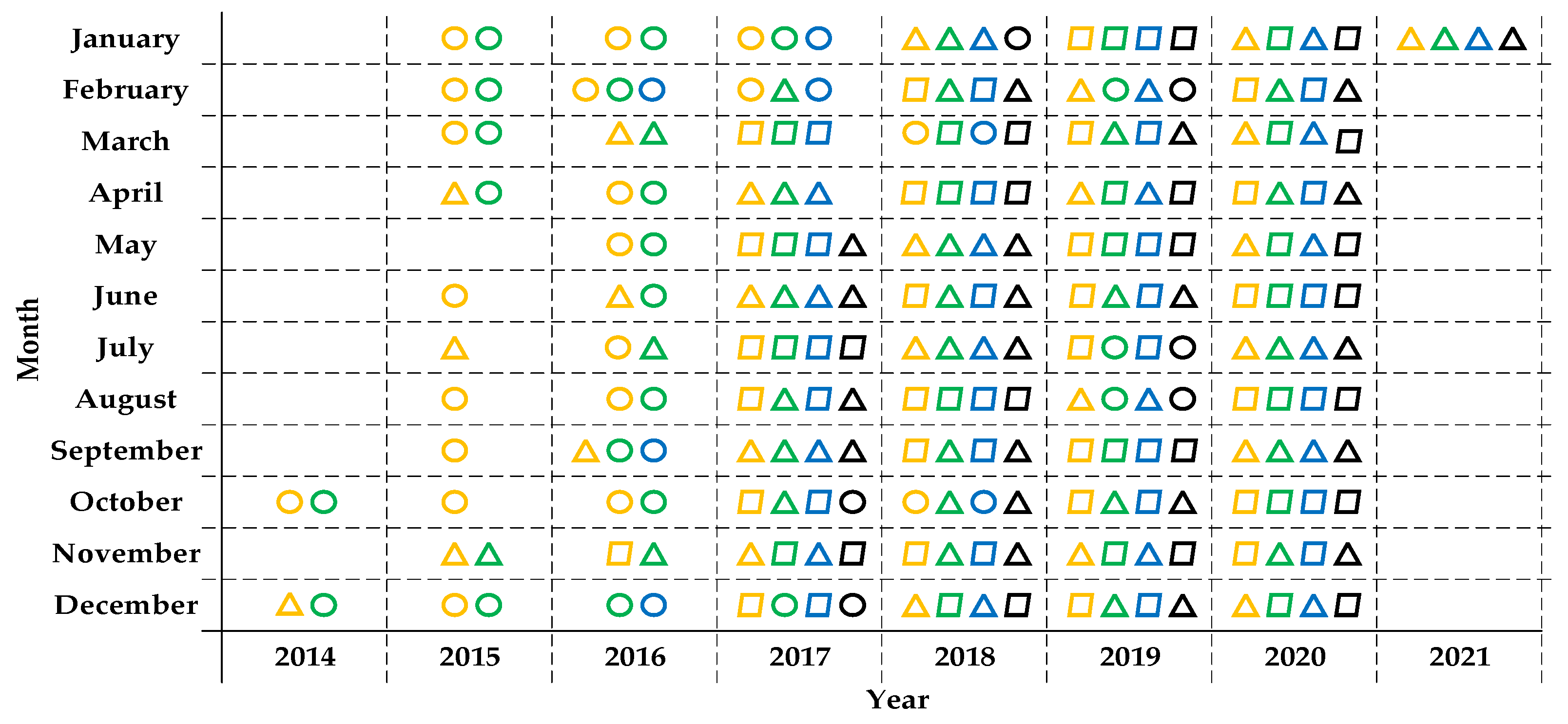
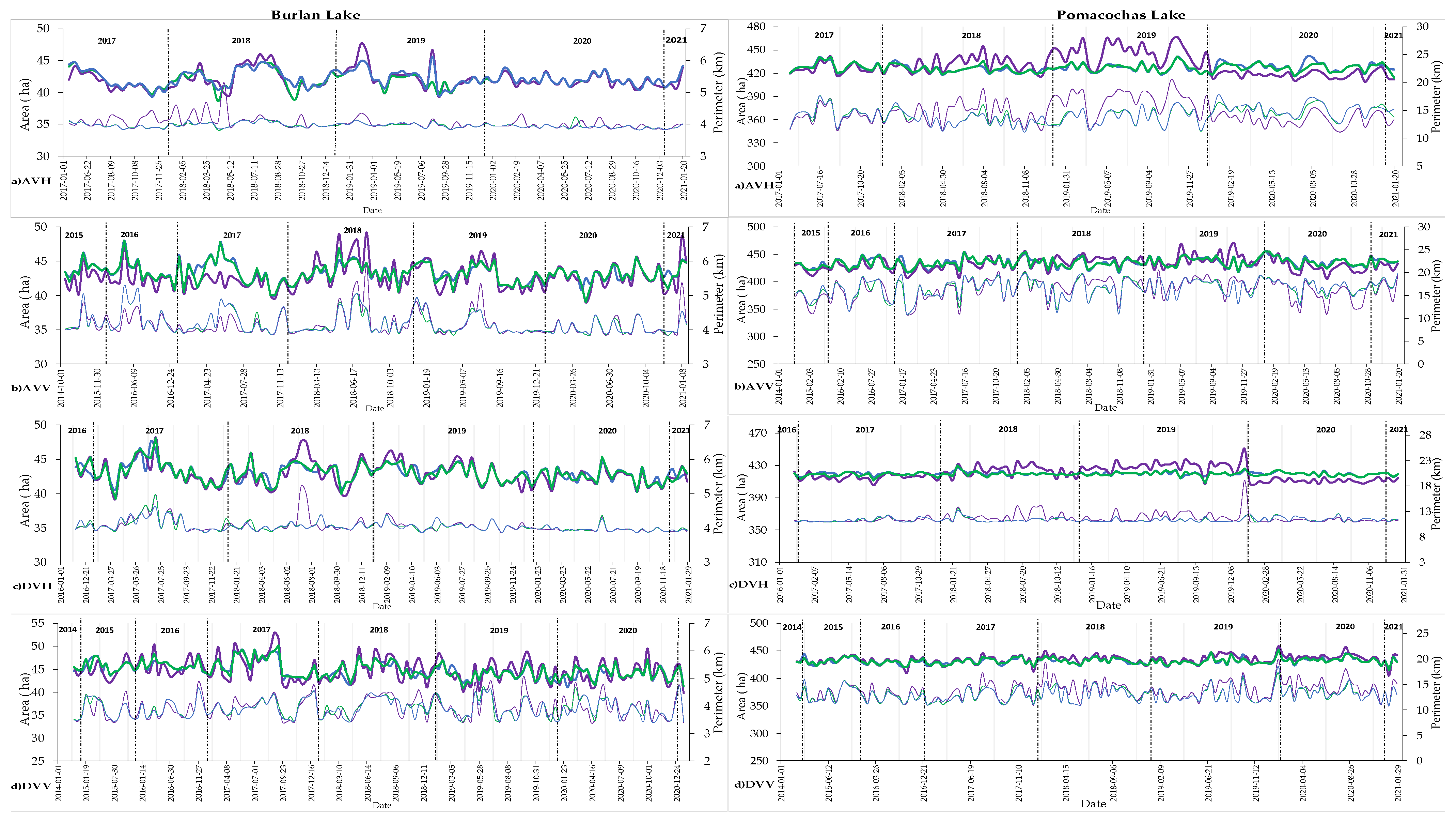
3.1. Distribution and Availability of SAR Data

Figure 4 shows the distribution and monthly availability of the SAR images used for the analysis of the dynamics of Burlan and Pomacochas Lakes from 2014–2021.

A total of 517 Sentinel-1 images were analysed for each study lake from 2014/10/06 to 2021/01/29 (

Table 1. Number of SAR images used to generate the water masks of Burlan and Pomacochas Lakes using CART, RF, and SVM.

Lake	SAR Images Available					Water Masks Analysed
	DVV 2014/10/15–2021/01/29	AVV 2014/10/06–2021/01/20	DVH 2016/02/07–2021/01/29	AVH 2017/05/17–2021/01/20	Total	CART	RF	SVM	Total
Burlan	153	137	123	104	517	517	517	517	1551
Pomacochas	153	137	123	104	517	517	517	517	1551
Total					1034				3102

). In addition, due to the classification using CART, RF, and SVM, 3 products were obtained per image, generating a total of 3102 water masks for both lakes.

Table S1 shows the attributes of all the images used to obtain the water masks of Burlan and Pomacochas Lakes from 2014–2021. We worked with the same scene because we used IW products (250 km for each sweep), and the distance between the lakes was approximately 50 km.

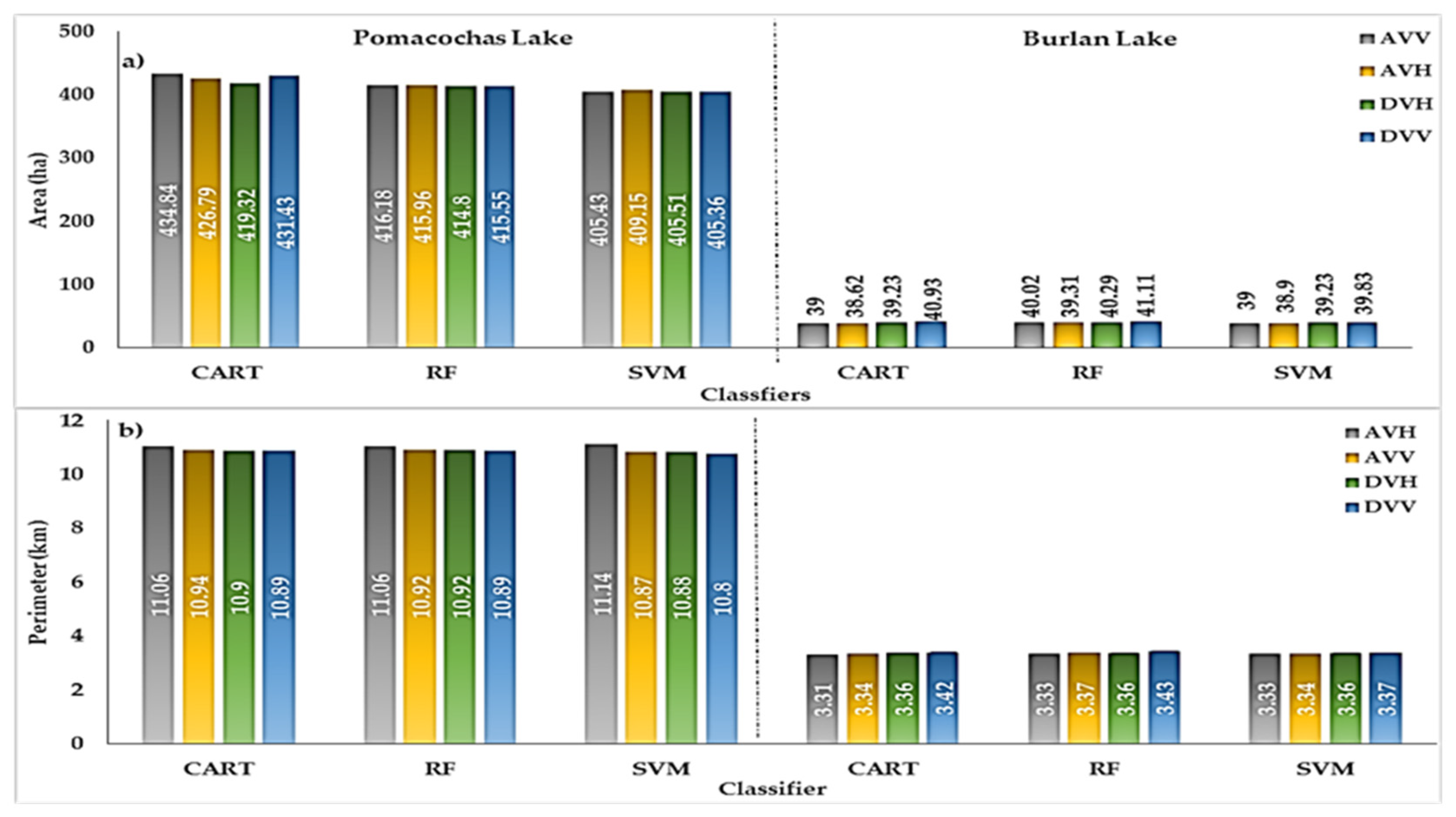
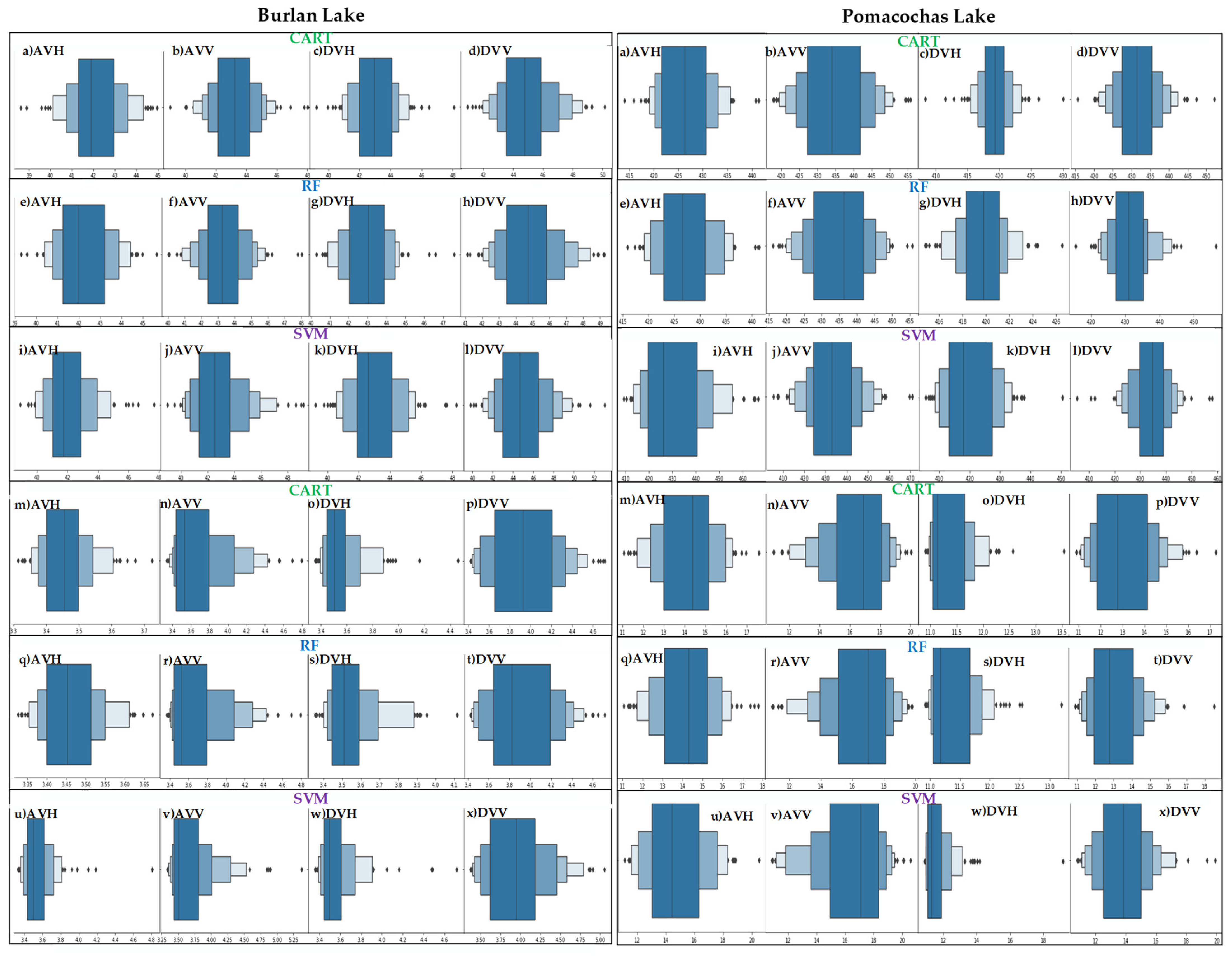
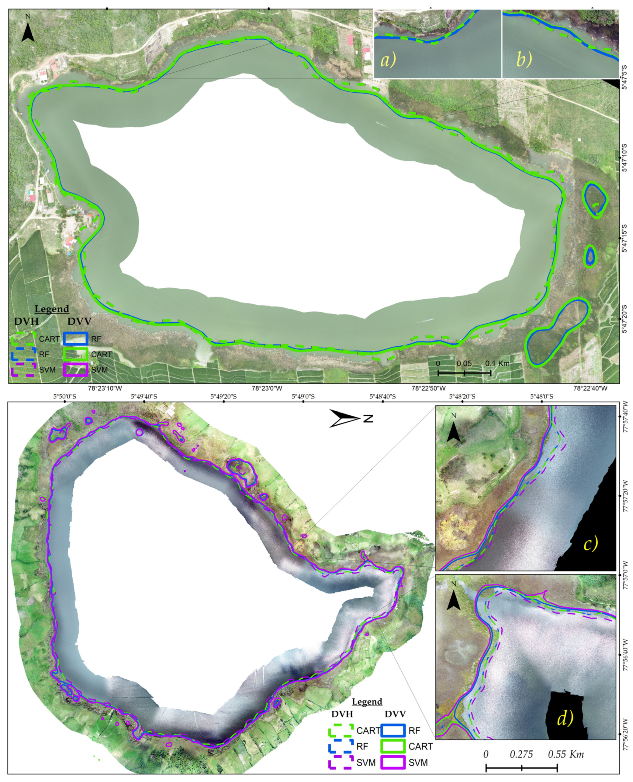
3.2. Obtaining the Geometric Attributes

Figure 5 shows the variation of area and perimeter for Burlan Lake (left) and Pomacochas (right). For Burlan Lake, the maximum values differ according to the flight direction and polarization, for example, 2018 and 2019 show maximum values for VH, while for VV, the maximum values are shown in 2016, 2017 and 2018. On the other hand, Pomacochas Lake presents a homogenous trend, for example, VH presents maximum values in 2018 and 2019, while VV presents a homogeneous trend with maximum values in 2019.

Table 2. Minimum, maximum, and average values of the area and perimeter of the Burlan and Pomacochas lakes obtained by classification of SAR images in the 2014–2020 period.

Classifier	Geometric Attribute		Burlan Lake				Pomacochas Lake
			AVH	AVV	DVH	DVV	AVH	AVV	DVH	DVV
Classification and regression tree(CART)	Area (ha)	Minimum	38.6	39	39.2	40.9	414	417.8	408.3	415.6
		Maximum	45	48	48.1	50.2	441.4	455.8	430.1	452.2
		Average	42.1	43.3	43	44.9	426.8	434.8	419.3	431.4
	Perimeter (km)	Minimum	3.31	3.34	3.36	3.42	11.06	10.94	10.9	10.89
		Maximum	3.72	4.8	4.46	4.72	17.59	20.06	13.54	17.26
		Average	3.46	3.67	3.55	3.93	14.16	16.52	11.36	13.03
Random Forest(RF)	Area (ha)	Minimum	39.3	40	40.3	41.1	416	416.2	414.8	415.6
		Maximum	45.6	48	47.6	49.3	441.4	455.8	426.5	456.5
		Average	42.2	43.3	43	44.8	427.2	435.1	419.7	431.3
	Perimeter (km)	Minimum	3.33	3.37	3.36	3.43	11.06	10.92	10.92	10.89
		Maximum	3.67	4.8	4.12	4.72	17.79	19.79	13.2	18.52
		Average	3.46	3.68	3.54	3.91	14.2	16.59	11.38	13.02
Support Vector Machine(SVM)	Area (ha)	Minimum	38.9	39	39.2	39.8	409.2	405.4	405.5	405.4
		Maximum	47.7	49.2	48.3	53	466.8	470.8	450.6	458
		Average	42.1	42.8	43	44.9	430.5	433.5	420.1	434.3
	Perimeter (km)	Minimum	3.33	3.34	3.36	3.37	11.14	10.87	10.88	10.8
		Maximum	4.81	5.73	4.72	5.05	20.52	20.58	19.17	19.92
		Average	3.55	3.66	3.57	3.95	14.72	16.43	11.65	13.86

shows the minimum, maximum and average values obtained for the area (A) and perimeter (P) of Burlan and Pomacochas Lakes calculated according to the classification of SAR images using CART, RF, and SVM. The behaviour of the values obtained by CART and RF was similar for both lakes, while the SVM values were much higher, due to the algorithm used in the classification.

Figure 6 compares the averaged values of the area (ha) and perimeter (km) of the Pomacochas and Burlan lakes for the combinations AVH, AVV, DVH, and DVV resulting from the classification of SAR images using CART, RF and SVM.

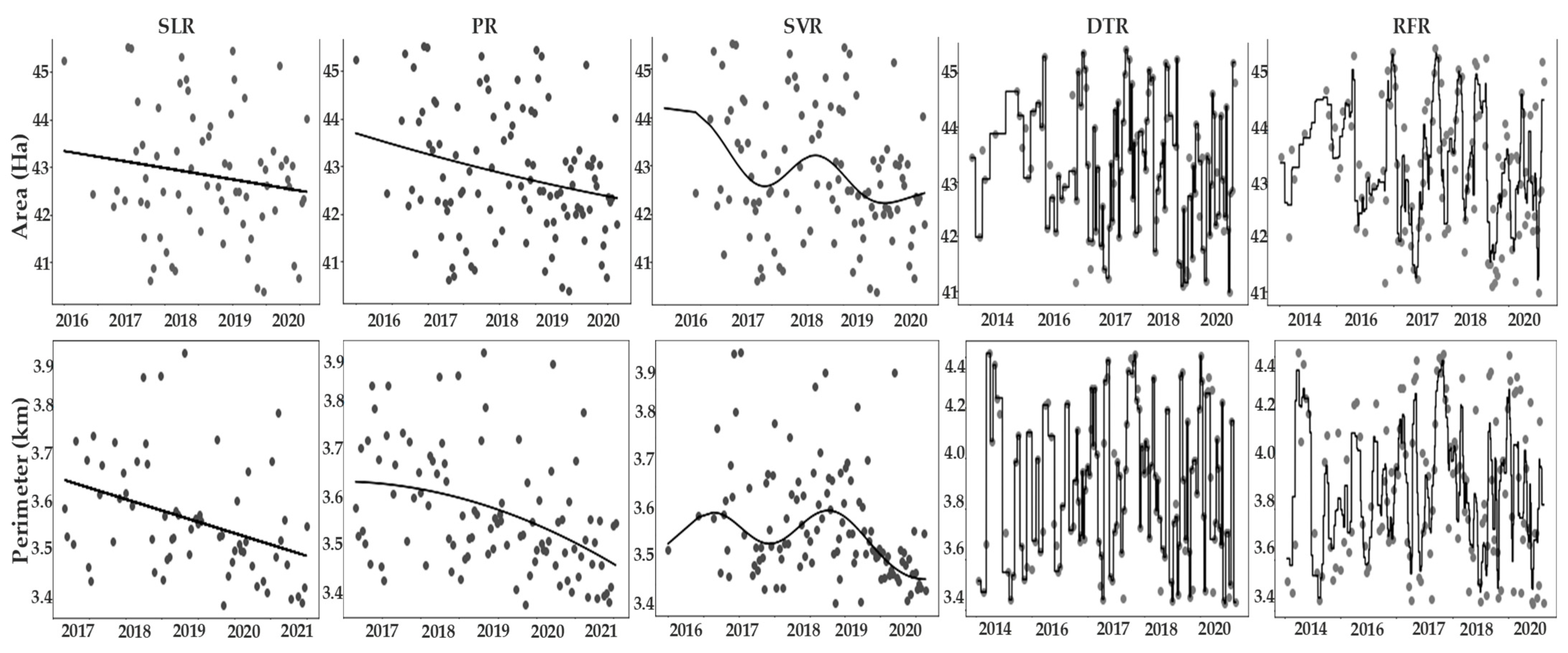
3.3. Data Analysis and Prediction

3.3.1. Data Normalization

For each combination, graphs of letter values (Boxenplots) were created in Google Colaboratory [50] because each batch of data was less than 200 elements [51].

Figure 7 shows the data distribution for each combination (AVV, AVH, DVV, and DVH), where the subfigures of a—l, m—x of each lake represent the data distributions of the area and perimeter, respectively.

As shown in Figure 7, there are outliers for each lake dataset. For example, in sub-figure (o) DVH of Burlan Lake, which represents the distribution of perimeter data obtained in Sentinel-1 descending pass and VH polarization, the majority of data are grouped from 3.4 to 3.6 km, but there are outliers that exceed 4 km (4.2 and 4.4). For its part, the data for Pomacochas Lake was also dispersed, for example, in sub-figure (i) AVH, most of the area data were grouped from 420 to 440 ha, but there are also values that exceed 460 ha and there are also values smaller than 415 ha. Therefore, to perform a correct regression analysis without the inclusion of outliers that can negatively impact the regression models, we proceeded to delete those values.

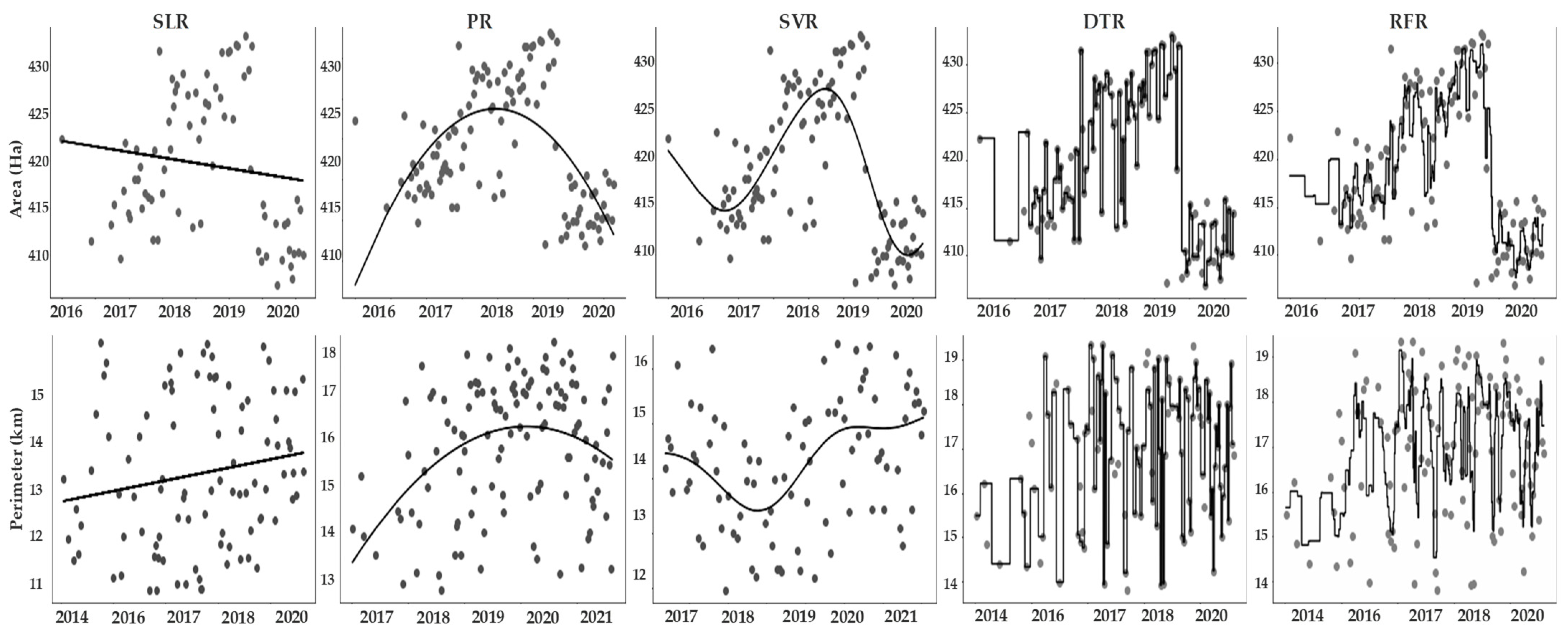
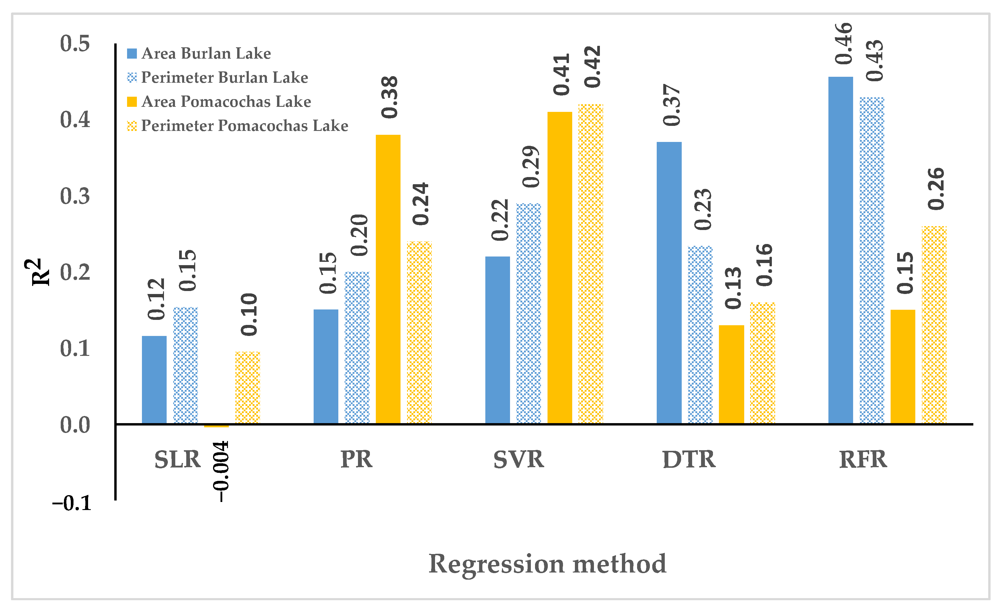
3.3.2. Regression Methods

Table 3. Area (ha) and perimeter (km) estimated with SLR, PR, SVR, DTR and RFR of greater R².

		SLR	PR	SVR	DTR	RFR
Burlan Lake	Area	42.46	42.3	42.43	45.2	44.47
	R2	0.12	0.15	0.22	0.37	0.46
	Combination	DVH	DVH	DVH	AVV	AVV
	Perimeter	3.43	3.41	3.41	3.43	3.82
	R2	0.15	0.2	0.29	0.23	0.43
	Combination	AVH	AVH	DVH	DVV	DVV
Pomacochas Lake	Area	417.8	408	411.42	414	413.1
	R2	-0.004	0.38	0.41	0.13	0.15
	Combination	DVH	DVH	DVH	DVH	DVH
	Perimeter	13.28	16.5	15.14	17.1	17.46
	R2	0.095	0.24	0.42	0.16	0.26
	Combination	DVV	AVV	AVH	AVV	AVV

shows the values of the area, perimeter, and coefficients of determination (R²) that had the highest degree of fit estimated according to SLR, PR, SVR, DTR, and RFR for 2021-02-10. Table S2 of the supplementary material shows all the R² calculated in the present investigation.

To complement Table 3, Figure 8 and Figure 9 show the best fit of the model to the area and perimeter data. For Burlan Lake, SLR, PR, and SVR were better fit to the area data of the DVH combination classified by SVM, while DTR and RFR were better fit to the AVV combination classified by CART. For the perimeter, SLR and PR was a better fit to the AVH combination classified by SVM, and SVR was a better fit to the DVH combination classified by SVM. Finally, DTR and RFR were a better fit for the DVV combination classified by CART. For Pomacochas Lake, all regression models were better fit to the area data of the DVH combination classified by SVM; for the perimeter, SLR was better fit to the DVV combination classified by CART, PR to AVV classified by SVM, SVR to AVH classified by RF, and finally, DTR and RFR to DVV classified by CART.

For Burlan Lake, with the AVV and DVV combinations classified by CART, RFR obtained the best R² for the area (0.46) and perimeter (0.43), respectively. In turn, for Pomacochas Lake, the combination DVH classified by SVM and AVH classified by RF obtained the best R² for the area (0.41) and perimeter (0.42), respectively, according to SVR.

Next, Figure 10 compares the R² of each regression method. It can be seen that for Burlan Lake, RFR showed higher R² in the area and perimeter data, thus showing an average adaptation of the model to the data, while for Pomacochas Lake the model that best fits the area and perimeter was the regression model by support vectors.

3.3.3. Validation

Figure 11 shows the polygons obtained from the classification of a SAR image of 2021-02-10, using CART (green), RF (blue) and SVM (purple) and overlaid with the orthomosaic of Burlan and Pomacochas lakes obtained by the RPAS on the same passage date.

The continuous lines were obtained from the classification of a descending combination SAR image in VV polarization (DVV), while the discontinuous lines are the result of the descending combination in VH polarization (DVH).

The orthomosaics had a mean RMS error of 0.043 m for pomacochas and 0.008 m for Burlan lake. The area (A) and perimeter (P) in hectares and kilometres, respectively, were calculated for each polygon extracted from the SAR image of the DVH and DVV combinations. These values were compared with the estimation by the best regression method and the flight with RPAS performed on Burlan and Pomacochas Lakes. In addition, the percentage of variation of the SAR image and the regression estimation were calculated with respect to the values obtained by the RPAS, as shown in

Table 4. Cross comparison of area and perimeter of SAR classification, the method of regression of higher R² with respect to photogrammetric flight.

SAR Image														Best Regressionmethod	∆%	RPAS
	DVV							DVH
		CART	∆%	RF	∆%	SVM	∆%	CART	∆%	RF	∆%	SVM	∆%
Burlan lake	A	43.53	−3.27	42.89	−4.69	43.42	−3.51	42.46	−5.64	42.48	−5.60	42.48	−5.60	44.47	−1.18	45.63
	P	3.4	−17.68	3.3	−20.10	3.38	−18.16	2.87	−30.51	2.87	−30.51	2.87	−30.51	3.82	−7.51	4.13
Pomacochas lake	A	434.89	1.35	430.77	0.39	437.18	1.89	420.57	−1.99	420.57	−1.99	414.23	−3.46	411.89	−4.01	429.09
	P	12.21	23.46	11.13	12.54	13.03	31.75	9.51	−3.84	9.49	−4.04	9.14	−7.58	17.46	76.54	9.89

.

4. Discussion

The monitoring of lakes using SAR images is very diverse, and commercial SAR products [6,52] or free access products such as those of the Sentinel-1 mission [28] can be used. In 2015, the launch of GEE [23] and the incorporation of the GRD products of Sentinel-1 facilitated the management of and access to SAR images. In this study, we used 517 Sentinel-1 A/B images for both lakes under study, having greater data availability as of 2016, we considered the period 2014–2020, as did Zijie et al. [53], but we calculated water masks by combining the polarizations and directions flight of the satellite. This approach was proposed because the retrospection in the images is different according to the direct flight or polarization considered; we based it on Table 4 and Figure 5.

To calibrate the first-level data of Sentinel-1, there are four look-up tables (LUTs). In the case of the level 1 files in Sentinel-1 GRD format, the zero sigma correction type is the most commonly used to generate the dispersion coefficient (σ°) [54]. To perform the correction of Sentinel-1 images, processes such as the application of orbit files, thermal noise removal, border noise removal, speckle filtering, and range-Doppler terrain correction are performed, all of which are performed in SNAP. In China, Zeng et al. [14] used this data processing approach for their research. For our part, we used the Sentinel-1 GRD products already available in GEE. This dataset provides images in which the pixel values are directly related to the backscatter of the radar by scene. That is, they are radiometrically calibrated, including thermal noise removal and terrain correction using Shuttle Radar Topography Mission (SRTM) and Advanced Spaceborne Thermal Emission and Reflection Radiometer (ASTER) digital elevation models (DEMs). Therefore, when using the GEE functions to homogenize the images, we opted to eliminate the noise using reducing filtering.

There are several ways to approach the extraction of water bodies from SAR images, for example, Otsu segmentation [55] and delineation through active contour models [56]. In this study, we used SAR images classified by three machine learning algorithms [32] to compare the results of the classification and to take advantage of the versatility and adaptability of GEE for the processing of SAR images, in addition to the parallel execution of the three algorithms CART, RF, and SVM.

Because similar studies have not been reported for the study lakes, we cannot compare the results of the classification, and we only lay the foundations for subsequent studies framed in the sixth sustainable development goal (target 6.6, indicator 6.6.1), which mentions that there are changes in the extent of water-related ecosystems over time [57].

Due to the geographical location of the study lakes, no marked trends were found with respect to monthly changes in area and perimeter, with the exception of the month of January, which is the month of greatest rainfall in the area. The area and perimeter values obtained by CART and Random Forest were similar, but the Support Vector Machine yields different values due to the input parameters of each algorithm, for example, the decision trees (CART and Random Forest) and the types of kernels (SMV) used in the classification. Several studies compare the performance of classifiers in different applications [58,59,60], and obtain different accuracies by simply modifying the number of decision trees or the type of kernel [61], so, at present, there are no defined parameters for image classification, and it is the task of each researcher to use and modify the input parameters. In our case, the accuracies were similar, but the values of the area and perimeter differed in some cases.

In China, Zijie et al. [53] found a slow upwards trend since 2014–2020 in Baiyangdian Lake and that the area of the lake was greater in spring and winter; in our case, the precipitation shows a similar behaviour with the area of Burlan lake, while for Pomacochas lake there is no defined trend regarding precipitation. Indeed, in Figure 12, we show the precipitation (mm/day) extracted from Climate Hazards Group InfraRed Precipitation with Station data (CHIRPS) for the study lakes.

We consider that in the high-resolution orthomosaic obtained by the RPAS, the contour of the lakes is better defined than in the SAR image, these overlapping errors at the edges of the lakes are due to the different spatial resolutions. Valdez-Lazalde et al. [62] used high (Ikonos and QuickBird-2) and medium-resolution (SPOT-4 and Landsat-7 ETM⁺) images for the estimation of the tree cover of a pine forest. In turn, Hernán et al. [63] found better results with aerial and satellite images of 1m and 2.44 m spatial resolution, respectively, for the estimation of biomass in vineyards. As shown in Figure 11 and Table 4, the area and perimeter values of the images with the VH band were lower because the waves that were transmitted vertically and those that return to the sensor horizontally are small. This means that the intensity of the VH band was lower than that of the VV band [64].

In Peru, especially for the Amazonas region, there is no geospatial information with high spatial resolution [65], which is why the regression analysis was limited regarding including other variables such as precipitation, evapotranspiration, and temperature, the same variables that influence the dynamics of a lake [66]. For the calculation of meteorological variables, established models can be used or calibrations can be performed to obtain greater precision in the estimation of these variables [67]. In this investigation, we tried to relate only the area and date of acquisition of the SAR image; for this purpose, the dates were transformed to ordinal numbers, and taking advantage of the robustness of the nonlinear regressors (RFR, SVR, and DTR), a correlation and predicted area and perimeter data with a mean R² fit (±0.4) were obtained.

Through the type of regression analysis used in this research, the area and perimeter values were similar to those of the validation with the RPAS, unlike the perimeter of Pomacochas lake, which was overestimated, in addition, the shape of the polygons extracted from the SAR images classified by our approach differs slightly with the shape of each lake, as shown in Figure 11. The variation in the contour shapes of each lake occurs because the spatial resolution of the RPAS used is much higher (50 cm/pixel) than that of Sentinel-1 (approximately 10 m/pixel).

The use of single polarizations can help to detect water bodies, but double polarizations have better performance [68,69]. In particular, we used dual polarizations, specifically the data obtained from VV polarization obtained better consistency according to SVR for Burlan Lake, while the VH polarization according to RFR for Pomacochas Lake. As shown in Figure 10, the maximum R² of the regression methods does not exceed 0.5, so data from different sensors can be used to correct this [70].

Generating geospatial information from optical data in areas of cloud cover is a challenge [71]. Additionally, analyzing the dynamics of lakes in the Amazonas using data from all the factors that influence a lake continues to be a challenge due to the temporal resolution (different acquisition dates), absence of historical climate data, and low density of meteorological stations, which are issues to be resolved in future research. It should be noted that there are various products that can be obtained from SAR images (vegetation indices, and interferograms), but our research was focused only on providing a rapid methodology for the analysis of the dynamics of two lakes using the area and perimeter and their correlation with the date of acquisition of the GRD-type SAR images.

5. Conclusions

Processing Sentinel-1 data in GEE is efficient, fast, and suitable for studies of lake dynamics located in areas with high cloud cover. In addition, the good spatial and temporal resolution of Sentinel-1 data is suitable for an analysis of changes in short periods, helping to show the multitemporal dynamics of water bodies. In particular, this research helped to show the variation in the area and perimeter of the Burlan and Pomacochas lakes, which was greater in the first months of each year.

On the other hand, GC was essential for quickly and easily executing five regression methods, showing that Random Forest Regression worked better both as a classifier and as a predictor. Variations of −1.18% and −7.51% were achieved with respect to the area and perimeter of Burlan Lake obtained through the Remote Pilot Aircraft System. On the other hand, for Pomacochas Lake, RFR underestimated the area of Pomacochas Lake by −4.01% and overestimated the value of the perimeter by 76.54%.

Finally, this research provided a general methodology for the processing of Sentinel-1 data to analyse water bodies, using Classification and Regression Trees, Random Forests and Support Vector Machines similar to a classifier. In addition, customizable scripts were provided for prediction using five regression methods in Google Colaboratory.

References

1. USGS Where Is Earth’s Water? Available online: https://www.usgs.gov/special-topic/water-science-school/science/where-earths-water?qt-science_center_objects=0#qt-science_center_objects (accessed on 10 April 2021).
2. Meyer, M.F.; Labou, S.G.; Cramer, A.N.; Brousil, M.R.; Luff, B.T. The global lake area, climate, and population dataset. Sci. Data 2020, 7, 1–12. [Google Scholar] [CrossRef]
3. Messager, M.L.; Lehner, B.; Grill, G.; Nedeva, I.; Schmitt, O. Estimating the volume and age of water stored in global lakes using a geo-statistical approach. Nat. Commun. 2016, 7, 13603. [Google Scholar] [CrossRef] [PubMed]
4. Lee, Z.; Shang, S.; Qi, L.; Yan, J.; Lin, G. A semi-analytical scheme to estimate Secchi-disk depth from Landsat-8 measurements. Remote Sens. Environ. 2016, 177, 101–106. [Google Scholar] [CrossRef]
5. Liu, J.; Yang, H.; Gosling, S.N.; Kummu, M.; Flörke, M.; Pfister, S.; Hanasaki, N.; Wada, Y.; Zhang, X.; Zheng, C.; et al. Water scarcity assessments in the past, present, and future. Earth’s Future 2017, 5, 545–559. [Google Scholar] [CrossRef]
6. Li, S.; Tan, H.; Liu, Z.; Zhou, Z.; Liu, Y.; Zhang, W.; Liu, K.; Qin, B. Mapping High Mountain Lakes Using Space-Borne Near-Nadir SAR Observations. Remote Sens. 2018, 10, 1418. [Google Scholar] [CrossRef] [Green Version]
7. Bioresita, F.; Puissant, A.; Stumpf, A.; Malet, J.P. Fusion of Sentinel-1 and Sentinel-2 image time series for permanent and temporary surface water mapping. Int. J. Remote Sens. 2019, 40, 9026–9049. [Google Scholar] [CrossRef]
8. Liao, H.-Y.; Wen, T.-H. Extracting urban water bodies from high-resolution radar images: Measuring the urban surface morphology to control for radar’s double-bounce effect. Int. J. Appl. Earth Obs. Geoinf. 2020, 85, 102003. [Google Scholar] [CrossRef]
9. Barasa, B.; Wanyama, J. Freshwater lake inundation monitoring using Sentinel-1 SAR imagery in Eastern Uganda. Ann. GIS 2020, 26, 191–200. [Google Scholar] [CrossRef] [Green Version]
10. Musa, Z.N.; Popescu, I.; Mynett, A. A review of applications of satellite SAR, optical, altimetry and DEM data for surface water modelling, mapping and parameter estimation. Hydrol. Earth Syst. Sci. 2015, 19, 3755–3769. [Google Scholar] [CrossRef] [Green Version]
11. Brisco, B. Mapping and Monitoring Surface Water and Wetlands with Synthetic Aperture Radar. Remote Sens. Wetl. Appl. Adv. 2015, 119–136. Available online: https://www.researchgate.net/profile/B-Brisco/publication/271765042_Remote_Sensing_of_Wetlands_Applications_and_Advances/links/59e4b1e1a6fdcc7154e140aa/Remote-Sensing-of-Wetlands-Applications-and-Advances.pdf (accessed on 15 October 2022).
12. Dewan, A.M.; Kankam-Yeboah, K.; Nishigaki, M. Using Synthetic Aperture Radar (SAR) Data for Mapping River Water Flooding in an Urban Landscape: A Case Study of Greater Dhaka, Bangladesh. J. Jpn. Soc. Hydrol. Water Resour. 2006, 19, 44–54. [Google Scholar] [CrossRef]
13. Nath, R.K.; Deb, S.K. Water-Body Area Extraction From High Resolution Satellite Images-An Introduction, Review, and Comparison. Int. J. Image Process. 2010, 3, 353–372. [Google Scholar]
14. Zeng, L.; Schmitt, M.; Li, L.; Zhu, X.X. Analysing changes of the poyang lake water area using sentinel-1 synthetic aperture radar imagery. Int. J. Remote Sens. 2017, 38, 7041–7069. [Google Scholar] [CrossRef]
15. Ding, X.W.; Li, X.F. Monitoring of the water-area variations of Lake Dongting in China with ENVISAT ASAR images. Int. J. Appl. Earth Obs. Geoinf. 2011, 13, 894–901. [Google Scholar] [CrossRef]
16. Costa, M.P.F.; Telmer, K.H. Utilizing SAR imagery and aquatic vegetation to map fresh and brackish lakes in the Brazilian Pantanal wetland. Remote Sens. Environ. 2006, 105, 204–213. [Google Scholar] [CrossRef]
17. Grunblatt, J.; Atwood, D. Mapping lakes for winter liquid water availability using SAR on the north slope of alaska. Int. J. Appl. Earth Obs. Geoinf. 2014, 27, 63–69. [Google Scholar] [CrossRef]
18. Nery, T.; Sadler, R.; Solis-Aulestia, M.; White, B.; Polyakov, M.; Chalak, M. Comparing supervised algorithms in Land Use and Land Cover classification of a Landsat time-series. In Proceedings of the International Geoscience and Remote Sensing Symposium (IGARSS), Beijing, China, 10–15 July 2016; Institute of Electrical and Electronics Engineers Inc.: Piscataway, NJ, USA, 2016; pp. 5165–5168. [Google Scholar]
19. Shetty, S. Analysis of Machine Learning Classifiers for LULC Classification on Google Earth Engine Analysis of Machine Learning Classifiers for LULC Classification on Google Earth Engine. Master’s Thesis, Universidad de Twente, Enschede, The Netherlands, 2019. [Google Scholar]
20. Liaw, A.; Wiener, M. Classification and Regression by randomForest. R News 2002, 2, 18–22. [Google Scholar]
21. Schapire, R.E.; Freund, Y.; Bartlett, P.; Lee, W.S. Boosting the margin: A new explanation for the effectiveness of voting methods. Ann. Stat. 1998, 26, 1651–1686. [Google Scholar] [CrossRef]
22. Breiman, L. Bagging Predictors. Mach. Learn. 1996, 2, 123–140. [Google Scholar] [CrossRef] [Green Version]
23. Gorelick, N.; Hancher, M.; Dixon, M.; Ilyushchenko, S.; Thau, D.; Moore, R. Google Earth Engine: Planetary-scale geospatial analysis for everyone. Remote Sens. Environ. 2017, 202, 18–27. [Google Scholar] [CrossRef]
24. Tamiminia, H.; Salehi, B.; Mahdianpari, M.; Quackenbush, L.; Adeli, S.; Brisco, B. Google Earth Engine for geo-big data applications: A meta-analysis and systematic review. ISPRS J. Photogramm. Remote Sens. 2020, 164, 152–170. [Google Scholar] [CrossRef]
25. Brownlee, J. Master Machine Learning Algorithms, 2016. Available online: https://machinelearningmastery.com/master-machine-learning-algorithms/(accessed on 15 October 2020).
26. SENAMHI Mapa Climático del Perú. Available online: https://www.senamhi.gob.pe/?p=mapa-climatico-del-peru (accessed on 22 October 2020).
27. Barboza-Castillo, E.; Maicelo-Quintana, J.L.; Vigo-Mestanza, C.; Castro-Silupú, J.; Oliva-Cruz, S.M. Análisis morfométrico y batimétrico del lago Pomacochas (Perú). Indes 2016, 2, 90–97. [Google Scholar] [CrossRef]
28. ESA Sentinel-1. Available online: https://sentinel.esa.int/web/sentinel/missions/sentinel-1 (accessed on 12 January 2021).
29. GEE Sentinel-1 Algorithms. Available online: https://developers.google.com/earth-engine/guides/sentinel1 (accessed on 15 January 2021).
30. Maitre, H. (Ed.) Processing of Synthetic Aperture Radar Images; ISTE Ltd Jhon Wiley & Sons, Inc.: Hoboken, NJ, USA, 2008; ISBN 978-1-84821-024-0. [Google Scholar]
31. GEE ee.Image.focal_median. Available online: https://developers.google.com/earth-engine/apidocs/ee-image-focal_median#javascript (accessed on 15 January 2021).
32. GEE Supervised Classification. Available online: https://developers.google.com/earth-engine/guides/classification (accessed on 22 January 2021).
33. Breiman, L. Random forests. Mach. Learn. 2001, 45, 5–32. [Google Scholar] [CrossRef]
34. Breiman, L.; Jerome, F.; Stone, C.J.; Olshen, R.A. Classification and Regresion Trees; Taylor & Francis Group: Abingdon, UK, 1984; ISBN 978-0-412-04841-8. [Google Scholar]
35. Burges, C.J.C. A tutorial on support vector machines for pattern recognition. Data Min. Knowl. Discov. 1998, 2, 121–167. [Google Scholar] [CrossRef]
36. Hsu, C.-W.; Chang, C.-C.; Lin, C.-J. A Practical Guide to Support Vector Classification 2003; Available online: https://www.bibsonomy.org/bibtex/2c04ef97dc3c3de168e684c3e4abe061b/jil (accessed on 15 October 2021).
37. Stehman, S.V. Selecting and interpreting measures of thematic classification accuracy. Remote Sens. Environ. 1997, 62, 77–89. [Google Scholar] [CrossRef]
38. Pedregosa, F.; Varoquaux, G.; Gramfort, A.; Michael, V.; Thirion, B.; Grisel, O.; Blondel, M.; Prettenhofer, P.; Weiss, R.; Dubourg, V.; et al. Scikit-learn: Machine Learning in Python. J. Mach. Learn. Res. 2011, 12, 2825–2830. [Google Scholar]
39. Altman, N.; Krzywinski, M. Association, correlation and causation. Nat. Methods 2015, 12, 899–900. [Google Scholar] [CrossRef] [PubMed] [Green Version]
40. Altman, N.; Krzywinski, M. Simple linear regression. Nat. Methods 2015, 12, 999–1000. [Google Scholar] [CrossRef] [PubMed]
41. sklearn.linear_model.LinearRegression. Available online: https://scikit-learn.org/stable/modules/generated/sklearn.linear_model.LinearRegression.html (accessed on 25 January 2021).
42. sklearn.preprocessing.PolynomialFeatures. Available online: https://scikit-learn.org/stable/modules/generated/sklearn.preprocessing.PolynomialFeatures.html (accessed on 25 January 2021).
43. sklearn.preprocessing.StandardScaler. Available online: https://scikit-learn.org/stable/modules/generated/sklearn.preprocessing.StandardScaler.html (accessed on 26 January 2021).
44. Vapnik, V.N. The Nature of Statistical Learning Theory; Springer: New York, NY, USA, 2000. [Google Scholar]
45. sklearn.svm.SVR. Available online: https://scikit-learn.org/stable/modules/generated/sklearn.svm.SVR.html (accessed on 25 January 2021).
46. Support Vector Regression (SVR) Using Linear and Non-Linear Kernels—Scikit-Learn 1.1.2 Documentation. Available online: https://scikit-learn.org/stable/auto_examples/svm/plot_svm_regression.html#sphx-glr-auto-examples-svm-plot-svm-regression-py (accessed on 5 October 2022).
47. sklearn.ensemble.RandomForestRegressor. Available online: https://scikit-learn.org/stable/modules/generated/sklearn.ensemble.RandomForestRegressor.html#examples-using-sklearn-ensemble-randomforestregressor (accessed on 25 January 2021).
48. sklearn.tree.DecisionTreeRegressor . Available online: https://scikit-learn.org/stable/modules/generated/sklearn.tree.DecisionTreeRegressor.html (accessed on 25 January 2021).
49. Metrics and Scoring: Quantifying the Quality of Predictions. Available online: https://scikit-learn.org/stable/modules/model_evaluation.html#regression-metrics (accessed on 26 January 2021).
50. seaborn.boxenplot. Available online: https://seaborn.pydata.org/generated/seaborn.boxenplot.html#seaborn.boxenplot (accessed on 25 March 2021).
51. Hofmann, H.; Kafadar, K.; Wickham, H. Letter-value plots: Boxplots for large data. Am. Stat. 2011, 22. [Google Scholar] [CrossRef]
52. Strozzi, T.; Wiesmann, A.; Kääb, A.; Joshi, S.; Mool, P. Glacial lake mapping with very high resolution satellite SAR data. Nat. Hazards Earth Syst. Sci. 2012, 12, 2487–2498. [Google Scholar] [CrossRef] [Green Version]
53. Jiang, Z.; Jiang, W.; Ling, Z.; Wang, X.; Peng, K.; Wang, C. Surface Water Extraction and Dynamic Analysis of Baiyangdian Lake Based on the Google Earth Engine Platform Using Sentinel-1 for Reporting SDG 6.6.1 Indicators. Water 2021, 13, 138. [Google Scholar] [CrossRef]
54. European Space Agency Radiometric Calibration of Level-1 Products. Available online: https://sentinel.esa.int/web/sentinel/radiometric-calibration-of-level-1-products (accessed on 26 September 2021).
55. Li, J.; Wang, S. An automatic method for mapping inland surface waterbodies with Radarsat-2 imagery. Int. J. Remote Sens. 2015, 36, 1367–1384. [Google Scholar] [CrossRef]
56. Horritt, M.S.; Mason, D.C.; Luckman, A.J. Flood boundary delineation from synthetic aperture radar imagery using a statistical active contour model. Int. J. Remote Sens. 2001, 22, 2489–2507. [Google Scholar] [CrossRef]
57. Indicators for the Sustainable Development Goals. Available online: https://sdg.data.gov/es/ (accessed on 24 May 2021).
58. Pande-Chhetri, R.; Abd-Elrahman, A.; Liu, T.; Morton, J.; Wilhelm, V.L. Object-based classification of wetland vegetation using very high-resolution unmanned air system imagery. Eur. J. Remote Sens. 2017, 50, 564–576. [Google Scholar] [CrossRef]
59. Statnikov, A.; Wang, L.; Aliferis, C.F. A comprehensive comparison of random forests and support vector machines for microarray-based cancer classification. BMC Bioinform. 2008, 9, 319. [Google Scholar] [CrossRef] [Green Version]
60. Liu, M.; Wang, M.; Wang, J.; Li, D. Comparison of random forest, support vector machine and back propagation neural network for electronic tongue data classification: Application to the recognition of orange beverage and Chinese vinegar. Sens. Actuators B Chem. 2013, 177, 970–980. [Google Scholar] [CrossRef]
61. Liu, T.; Abd-Elrahman, A.; Morton, J.; Wilhelm, V.L. Comparing fully convolutional networks, random forest, support vector machine, and patch-based deep convolutional neural networks for object-based wetland mapping using images from small unmanned aircraft system. GISci. Remote Sens. 2018, 55, 243–264. [Google Scholar] [CrossRef]
62. Valdez-Lazalde, J.R.; González-Guillén, M.d.J.; de los Santos-Posadas, H.M. Estimación de cobertura arbórea mediante imágenes satelitales multiespectrales de alta resolución. Agrociencia 2006, 40, 383–394. [Google Scholar]
63. Vila, H.; Perez Peña, J.; García, M.; Vallone, R.C.; Mastrantonio, L.; Olmedo, G.F.; Rodríguez Plaza, L.; Salcedo, C. Congreso Internacional de la AET. “Teledetección Hacia un Mejor Entendimiento de la Dinámica Global y Regional”; Estación Experimental Agropecuaria Mendoza INTA: Mendoza, Argentina, 2007. [Google Scholar]
64. Moreira, A.; Prats-Iraola, P.; Younis, M.; Krieger, G.; Hajnsek, I.; Papathanassiou, K. A Tutorial on Synthetic Aperture Radar. IEEE Geosci. Remote Sens. Mag. 2013, 1, 6–43. [Google Scholar] [CrossRef] [Green Version]
65. Yunis, C.R.C.; López, R.S.; Cruz, S.M.O.; Castillo, E.B.; López, J.O.S.; Trigoso, D.I.; Briceño, N.B.R. Land Suitability for Sustainable Aquaculture of Rainbow Trout (Oncorhynchus mykiss) in Molinopampa (Peru) Based on RS, GIS, and AHP. ISPRS Int. J. Geo-Inf. 2020, 9, 28. [Google Scholar] [CrossRef] [Green Version]
66. Jin-Ming, Y.; Li-Gang, M.; Cheng-Zhi, L.; Yang, L.; Jian-li, D.; Sheng-Tian, Y. Temporal-spatial variations and influencing factors of Lakes in inland arid areas from 2000 to 2017: A case study in Xinjiang. Geomat. Nat. Hazards Risk 2019, 10, 519–543. [Google Scholar] [CrossRef]
67. Valipour, M. Calibration of mass transfer-based models to predict reference crop evapotranspiration. Appl. Water Sci. 2017, 7, 625–635. [Google Scholar] [CrossRef] [Green Version]
68. Irwin, K.; Braun, A.; Fotopoulos, G.; Roth, A.; Wessel, B. Assessing Single-Polarization and Dual-Polarization TerraSAR-X Data for Surface Water Monitoring. Remote Sens. 2018, 10, 949. [Google Scholar] [CrossRef] [Green Version]
69. Scott, K.A.; Xu, L.; Pour, H.K. Retrieval of ice/water observations from synthetic aperture radar imagery for use in lake ice data assimilation. J. Great Lakes Res. 2020, 46, 1521–1532. [Google Scholar] [CrossRef]
70. Vickers, H.; Malnes, E.; Høgda, K.-A. Long-Term Water Surface Area Monitoring and Derived Water Level Using Synthetic Aperture Radar (SAR) at Altevatn, a Medium-Sized Arctic Lake. Remote Sens. 2019, 11, 2780. [Google Scholar] [CrossRef]
71. Zhang, H.; Zhang, Y.; Lin, H. A comparison study of impervious surfaces estimation using optical and SAR remote sensing images. Int. J. Appl. Earth Obs. Geoinf. 2012, 18, 148–156. [Google Scholar] [CrossRef]
Figure 1. Geographic location of the study lakes in NW Peru.
Ijgi 11 00534 g001
Figure 2. Methodological design for analysing the dynamics of the water surface of Burlan and Pomacochas Lakes during 2014–2020 using SAR images. * This procedure was performed internally by GEE.
Ijgi 11 00534 g002
Figure 3. Methodological flow for the regression analysis.
Ijgi 11 00534 g003
Figure 4. Distribution and monthly availability of the Sentinel-1 images used for the analysis of the dynamics of Burlan and Pomacochas Lakes from 2014 to 2021. The geometric figures represent the number of images available in a month, where circles, triangles, and parallelograms represent 1, 2, and 3 images, respectively. In addition, the colour of each represents the combination of the direction of passage and polarization, where orange, green, blue, and black represent the combinations of DVV, AVV, DVH, and AVH, respectively.
Ijgi 11 00534 g004
Figure 5. Variation in the area and perimeter of the Burlan and Pomacochas lakes using CART, RF, and SVM as classifiers of the SAR images. The thick lines represent the area (ha), and the thin lines represent the perimeter (km). In addition, the purple, green and blue lines represent the values obtained by SVM, CART and RF, respectively. In addition, AVH, AVV, DVH and DVV, represents the dataset obtained by: flight directions Ascending (A) and Descending (D), polarizations transmitted and received vertically (VV) and transmitted vertically and received horizontally (VH).
Ijgi 11 00534 g005
Figure 6. Average values of the (a) area and (b) perimeter of Pomacochas and Burlan Lakes.
Ijgi 11 00534 g006
Figure 7. Dispersion of the area and perimeter data for Burlan and Pomacochas Lakes, where the black points represent outliers, and the rectangles represent the highest clustering of data according to quantiles.
Ijgi 11 00534 g007
Figure 8. Regression models with greater R2 for the area and perimeter data of Burlan Lake.
Ijgi 11 00534 g008
Figure 9. Regression models with higher R2 for the area and perimeter data of Pomacochas Lake.
Ijgi 11 00534 g009
Figure 10. Comparison of the R2 calculated for the models of SLR, PR, SVR, DTR, and RFR.
Ijgi 11 00534 g010
Figure 11. Overlapping of the SAR classification and orthomosaic of Burlan (top) and Pomacochas (bottom) Lakes for 2021-02-10, and subfigures (ad) represent a zooming of each zone to visualize the classification result on the RPAS orthomosaic.
Ijgi 11 00534 g011
Figure 12. Daily distribution of precipitation for (a) Burlan and (b) Pomacochas lakes.
Ijgi 11 00534 g012