Morphometric Prioritization, Fluvial Classification, and Hydrogeomorphological Quality in High Andean Livestock Micro-Watersheds in Northern Peru

Abstract

Anthropic activity affects the hydrogeomorphological quality of fluvial systems. River and valley classifications are fundamental preliminary steps in determining their ecological status, and their prioritization is essential for the proper planning and management of soil and water resources. Given the importance of the High Andean livestock micro-watershed (HAL-MWs) ecosystems in Peru, an integrated methodological framework is presented for morphometric prioritization that uses a Principal Component Analysis (PCA) and Weighted Sum Approach (WSA), geomorphological fluvial classifications (channel, slope, and valley), and hydrogeomorphological evaluations using the Hydrogeomorphological Index (IHG). Of six HAL-MWs studied in Leimebamba and Molinopampa (Amazonas region), the PCWSA hybrid model identified the San Antonio HAL-MW as a top priority, needing the rapid adoption of appropriate conservation practices. Thirty-nine types of river course were identified, by combining 13 types of valley and 11 types of riverbed. The total assessment of the IHG indicated that 7.6% (21.8 km), 14.5% (41.6 km), 27.9% (80.0 km), and 50.0% (143.2 km) of the basin lengths have “Poor”, “Moderate”, “Good”, and “Very good” quality rankings, respectively. The increase in the artificial use of river channels and flood plains is closely linked to the decrease in hydrogeomorphological quality.

1. Introduction

In 2011, 11% of Earth’s surface and 70% of water extracted from aquifers, rivers, and lakes were purposed for agriculture [1]. By 2050, a world population of 9.1 billion [2] and a 70% increase in food production, compared to 2009, is estimated, which will have a direct impact on land and water resource availability [3]. Thirty-one percent of Earth’s 35 million km³ fresh water resources, on which aquatic and terrestrial ecosystems as well as mankind and diversity depend, are concentrated in Latin America and the Caribbean [4]. In Peru, the average availability of renewable water sources was 65.726 m³/inhabitant/year in 2016, ranking 17th out of 180 countries [5]. However, this availability does not correspond to the spatial distribution of the population, is non-uniform in time (mainly because of variable precipitation) and has decreased due to population growth [5,6]. These circumstances have resulted in scarcity and water stress, thus generating social and productive inequalities [5,7]. Moreover, socioeconomic changes and the accumulation of environmental problems exceed the pace of institutional responses [5].

Socioeconomic activities impact fluvial systems [8]. These activities generate both point and diffuse sources of contamination, morphological alterations, regulation, water extraction, the occupation of floodplains, the retention and extraction of solid flows [8], the proliferation of invasive species [9], and the modification and loss of the riverbank forest [10], among other consequences. These impacts are a result of external elements, such as gabions, dams [11], bridges [12,13], and also of disruptive activities including transfers [14], discharges, aggregate extraction, dredging, channeling, channel diversions, and the use of the land for urbanization [15], mining [16], plantations, landfills and dumps, transport routes [17], and grazing [18]. In summary, alteration is caused by (i) hydrological denaturalization; (ii) reduced sediment transport; (iii) the functional reduction of floodplains; (iv) direct action over the river channel, river bottom, and riverbank morphology; (v) and the deterioration of the flow, width, structure, naturalness, and connectivity of the river corridor [8].

Such impacts directly affect principal fluvial functions (the transport of water, sediment, nutrients, and organisms) and natural hydrogeomorphological processes (erosion, transport, and sedimentation) of the river system [19,20,21]. Land use also has important impacts on river systems, but particularly on small river basins that have a steeper slope and channel coupling than the riverbeds below [22]. In these micro-basins, cattle and sheep grazing tend to impact large geographical areas and produce geomorphic repercussions through trampling, which leads to soil compaction, accelerated runoff and gullying, riverbed vegetation disturbance, riverbed chiseling and detachment, the disruption of protective soil crusts, and the formation of terraces [18]. There are various ecological studies [23] of the deforestation of forests [24,25,26,27], weeds [28], the physicochemical properties of the soil [29,30,31], macroinvertebrates, and the physicochemical and microbiological properties of water [32,33,34,35,36], as evidence of the degradation of the high Andean livestock micro-basins in the Amazon region (in northern Peru). However, the hydrogeomorphological approach has been scarcely studied [37,38], as in all of Peru [39].

In this framework, hydrogeomorphology takes into account river channel processes and characteristics for the purpose of river management and restoration [40,41]. In Europe, numerous hydrogeomorphological methodologies have been developed, mainly after the launch of the European Union Water Framework Directive (DMA; 2000/60/CE) [42]. One hundred and twenty-one methods created in Europe, Africa, and the US have been created, tested, and revised from 1983 to 2013 [43]. For example, the Hydrogeomorphological Index (IHG) was developed in 2007 [19] and successfully applied in Spanish river channels [44,45]. It was consequently modified [46] and applied in other basins in Spain [47,48] and also adapted by South American countries such as Argentina [49], Chile [50,51], and Peru [37,38]. In Peru, there is no framework for river system hydrogeomorphological evaluation, but establishing such a framework is of primary importance due to the rugged high Andean territory and high non-uniform rainfall, which promote highly dynamic river behavior, in space and time.

Hydrogeomorphological evaluations, or any other fluvial studies, must begin with river channel and valley classification [52]. This process has been traditionally carried out in accordance with hydrological (ephemeral, intermittent, seasonal, permanent, etc.) and biological parameters, without taking into account geomorphological parameters [53]. However, the latter is more applicable and consistent with an hydro-morphological evaluation [52]. Internally and functionally homogenous river sections are quickly and easily identified according to geomorphological parameters, with data obtained by Remote Sensing (RS) and Geographic Information System (GIS) tools [53,54]. In the 21st century, methodologies proposed by Ollero et al. [55], Díaz and Ollero [54], Horacio and Ollero [53], Horacio et al. [56], and the most recent proposal by Horacio et al. [57], which uses lithological and topographic units (Lithotopo), stand out.

As such, the rugged High Andean topography and high rainfall conditions favor erosion-induced soil degradation [58]. In Peru, High Andean average erosion rates (162 tn/ha/year, from 1981 to 2014) were estimated with the use of the Revised Universal Soil Loss Equation (RUSLE) model [59]. In addition to the application of the RUSLE model, erosion-prone watersheds are evaluated and prioritized worldwide based on the Sediment Yield Index (SYI) [60], land use, land cover, morphometric variables, etc. The latter is more feasible, because it evaluates and prioritizes watersheds even without the soil map or land cover/use map [61]. Based on morphometric variables obtained from RS and GIS, several researchers have prioritized river basins by ordinary methods such as: Fuzzy Analytical Hierarchy Process (FAHP) [62], Principal Component Analysis (PCA) [63], and the Weighted Sum Approach (WSA) [64]. Nonetheless, a recent hybrid PCA and WSA methodology (PCSWSA), has proven to be an optimal strategy for micro-basin prioritization [65].

In this study, an integrated methodological framework for morphometric prioritization, geomorphological river classification, and the hydrogeomorphological evaluation of hydrographic basins is presented. This methodology was applied on six High Andean livestock micro-basins (HAL-MW) of high environmental and economic importance located in Leimebamba (Atuén, Cabildo, Pomacochas and Timbambo) and Molinopampa (San Antonio and Ventilla) in Amazonas (northern Peru). Consequently, (a) the land cover and uses of each HAL-MW were delimited and identified; (b) the HAL-MWs were prioritized according to morphometric variables (linear, areal, and morphology) and multivariate statistics; (c) the river network was classified based on geomorphological aspects (riverbed geomorphology, slope, and valley geomorphology); and (d) an IHG Index was applied for each river section that was classified as internally and functionally homogeneous. Ultimately, this research seeks to provide decision-making tools for river system management and restoration.

2. Materials and Methods

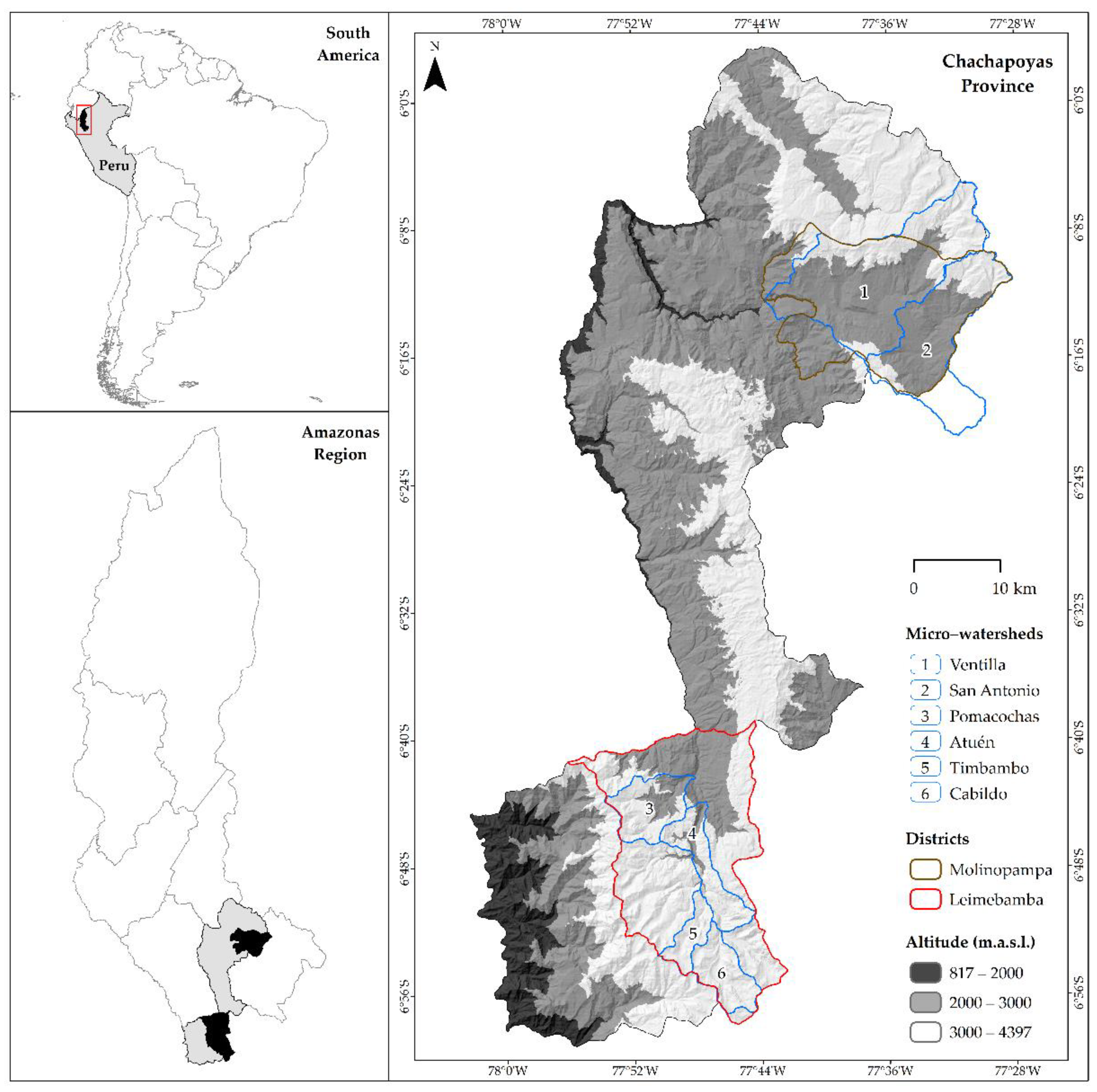
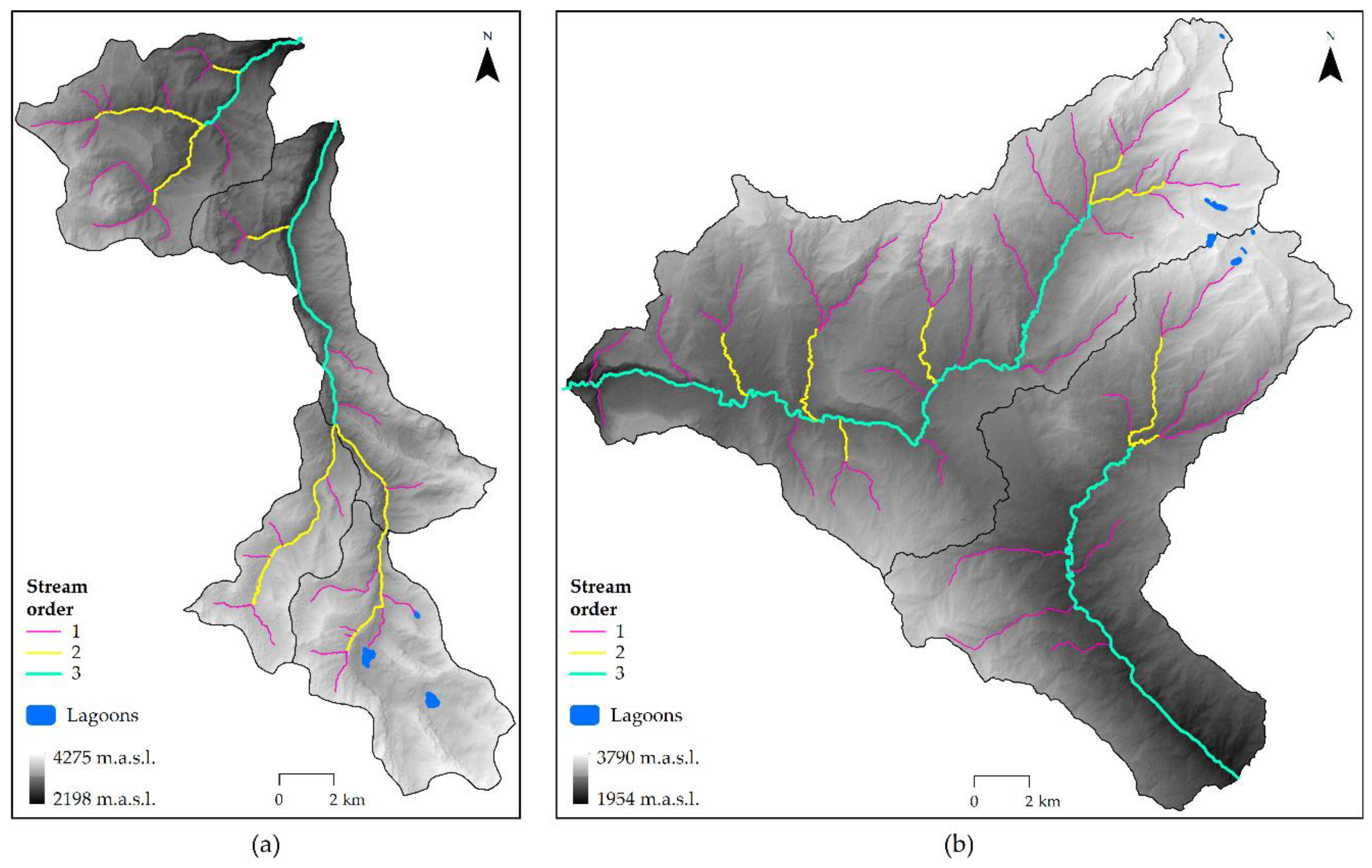
2.1. Study Area

Our study area corresponding to Northern Peru’s Amazonas region has an approximate surface area of 39.25 km², much of it covered by unexplored tropical forests. It is geographically located between parallels 3°0′15″, 7°2′0″ south latitude and meridians 77°0′15″ and 78°42′15″ west longitude, with an altitudinal gradient between 120 m.a.s.l. in the north, where humid lowland tropical forests predominate, and 4900 m.a.s.l. to the south where humid highland Andean tropical forests, cloud forests, and deforested grasslands predominate. Agriculture is the main economic activity in Amazonas, occupying 24.9% of the territory and being responsible for 51.22% of the regional Gross Domestic Product (GDP) [66]. There are four areas dedicated to livestock in the region [67]: (1) Pomacochas–Jumbilla, (2) Molinopampa–Mendoza, (3) Leimebamba, and (4) Chiriaco. The first three zones are located in areas of cold temperate climate, where dairy cattle predominate; while the last zone, which has a warm and humid climate, is dedicated to raising Zebu cattle. In Leimebamba and Molinopampa, situated in the province of Chachapoyas (Figure 1), open-field cattle raising (extensive cattle farming) is executed alongside the Andean crop farming of potatoes, corn, and beans [68]. These areas include HAL-MW, belonging to the Utcubamba River level 5 Hydrographic Unit (HU N5) [37], located on slopes and mountain tops with altitudes exceeding 2000 m.a.s.l. They cover large areas of Andean grasslands and scrublands, used as natural pastures managed by anthropic burning [67], which in some cases is complemented by the planting of small pasture areas and forages near stables used for young bovine management. In that regard, Chachapoyas is noteworthy for being an exceptionally suitable area for dairy and beef cattle farming, to such an extent that 42.22% of the economically active population is dedicated to the aforementioned activities [68]. However, as a result of poor agricultural practices, unsustainable logging, urban expansion, and the construction of road infrastructure, these high Andean ecosystems are being degraded [23,24,25,26,27,28,29,30,31,32,33,34,35,36,37,38].

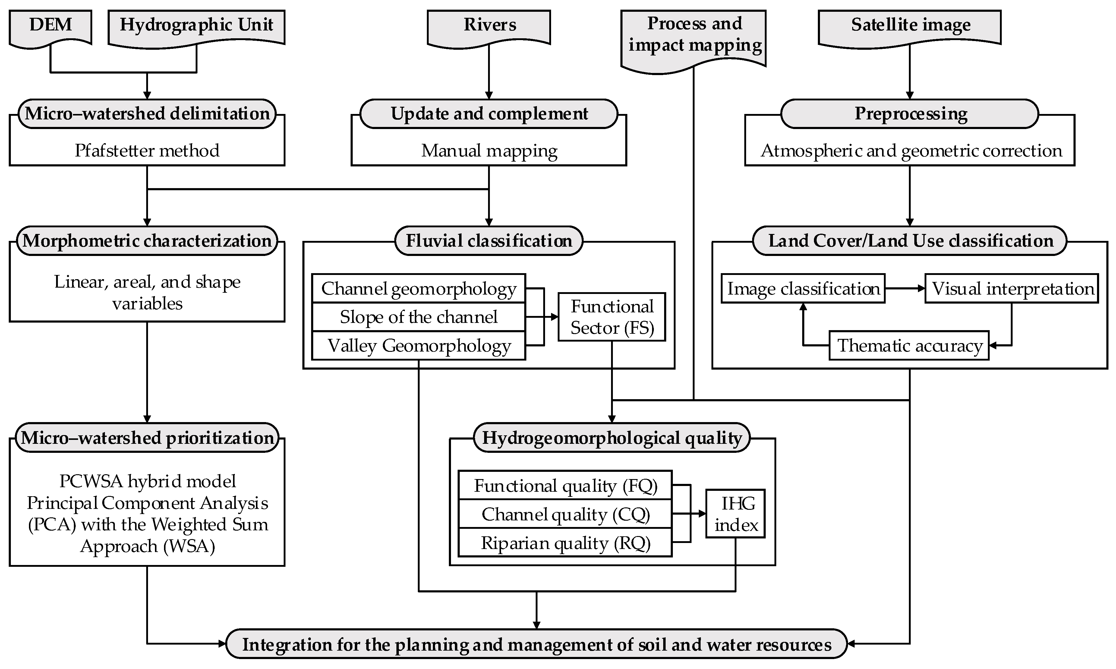
2.2. Methodological Design

This study constitutes the first integration of the three methodologies just described [19,53,65] to prioritize and evaluate hydrogeomorphological quality in high Andean watersheds. Figure 2 illustrates the methodological process developed for the morphometric prioritization process using PCWSA, geomorphological fluvial classification, and hydrogeomorphological quality evaluation through the use of the IHG in six HAL-MWs in northern Peru.

2.3. Base Map and Satellite Framework

To construct the base map and satellite framework, we utilized the HU N5 of the Utcubamba River, contained in the Peruvian hydrographic watershed vector layer, obtained from the National Water Authority’s (ANA) Geo-hydro portal [69]. Populated centers and the hydrography from the digitized 13h, 13i, and 14h quadrangles in the National Geographic Institute (IGN) topographical map series (scale of 1:100,000) were downloaded from the Ministry of Education’s web portal [70]. Road and bridge infrastructure data were obtained from the Transport and Communication Ministry’s website [71]. The Digital Elevation Model (DEM), generated by the Phased Array Type L-band Synthetic Aperture Radar (PALSAR) of Advanced Land Observing Satellite (ALOS) [72] from the Japan Aerospace Exploration Agency (JAXA), was also utilized. The data were downloaded from the National Aeronautics and Space Administration’s (NASA) ASD Data Search Vertex web portal [73], with a 12.5 meter spatial resolution. To generate the Coverage and Land Use (LC/LU) maps, we used two images with a spatial resolution of 10 meters acquired on July 23rd, 2017 from the Sentinel 2A satellite, Path 17, and Row MRP and MRN. These were acquired from the European Space Agency’s (ESA) Copernicus Services Data Hub platform, through QGIS’s Semi-Automatic Classification Plugin (SCP) [74].

2.4. Micro-Watershed Delimitation

Delimitation of the HAL-MWs was done using the DEM and coded from the Utcubamba River HU N5. This process was based on the Pfafstetter method [75,76] while using PgHydro Tools, a QGIS (version 2.18.10) plugin [77], to activate the PgHydro Extension functions for PostgreSQL/PostGIS. The linear water network layer was imported from Google Earth Pro (version 7.3.2.5576) and SAS Planet (version 190707) interfaces, and subsequently updated and complemented with manual mapping [78,79]. This procedure was critical in obtaining the detailed geomorphology of the channel at the micro-watershed level, because the base layer brought the smoothed and generalized rivers (scale 1:100000).

2.5. Micro–Watershed Priorization Model

HAL-MW prioritization was carried out based on linear, areal, and shape morphometric variables using the PCWSA hybrid model proposed by Malik et al. [65]. The linear variables that were measured were: maximum and minimum height (Hmax, Hmin), area (A), perimeter (P), basin length (Lb), Strahler order (u), length (L), slope of the main stream (Sl), stream length (Lu), stream length mean (Lsm), and the Bifurcation ratio (Rb), which depends on Lu and the total number of streams of order u (Nu) (

Table 1. Linear, areal, and shape morphometric variables and computation formulae with references.

Variables	Symbology	Unit	Formula	References
Linear Variables
Maximum altitude	Hmax	m.a.s.l.	Maximum altitude of watershed
Minimum altitude	Hmin	m.a.s.l.	Minimum altitude of watershed
Basin perimeter	P	km	Perimeter of watershed
Basin area	A	km2	Plan area of watershed
Stream order	u		Hierarchical rank	[80]
Total of flows of the order u	Nu		Total number of streams of order u	[81]
Stream length	Lu	km	Total length of stream of order u	[81]
Mean stream length	Lsm	km	Lu/Nu	[81]
Length of the main channel	L	km	Length of the main channel	[82]
Slope of the main channel	Sl	%	(Hmax of the main channel − Hmin)/L	[82]
Basin length	Lb	km	1.312 × A0.568	[83]
Bifurcation ratio	Rb		Nu/(Nu + 1)	[84]
Areal Variables
Mean slope of the basin 1	Sb	%	ΔH × ΣLl/A	[82]
Drainage density	Dd	km/km2	ΣLu/A	[85]
Stream frequency	Fs	km−2	ΣNu/A	[85]
Texture ratio	Rt	km−1	ΣNu/P	[81]
Mean length of overland Flow	Lom	km	1/2Dd	[81]
Shape Variables
Form factor	Ff		A/Lb2, Ff < 1	[85]
Circularity ratio	Rc		4πA/P2, RC ≤ 1	[86]
Compactness coefficient	Cc		0.2821P/A0.5, Cc ≥ 1	[80]
Elongation ratio	Re		1.128A0.5/Lb, Re ≤ 1	[84]

¹ΔH and ΣLl are the equidistance and the total length of the contour lines that pass through the basin, respectively.

). The areal variables were: the mean slope of the basin (Sb), drainage density (Dd), stream frequency (Fs), texture ratio (Rt), and mean length of the overland flow (Lom) (Table 1). The analyzed shape variables were: the form factor (Ff), Circularity ratio (Rc), Compactness coefficient (Cc), and Elongation ratio (Re) (Table 1).

Preliminary Priority Ranks (PPR) were assigned to each HAL-MW, with the use of one linear variable (Rb), four areal variables (Dd, Fs, Rt, Lom), and four shape variables (Ff, Rc, Cc, Re) [58,64,65]. Higher values of linear and area variables indicate a greater potential for soil erosion (direct relationship), while morphometric shape variables have an inverse relationship. Therefore, the highest erosion potential of these variables was assigned rank 1 (highest priority), the next highest potential value was assigned rank 2, and so forth for all HAL-MWs [58,61]. The correlation matrix, the first Load Factor (FL), and the rotated FL of the nine morphometric variables were constructed using PCA. This allowed us to identify the most significant morphometric variables. The PCA was performed using the SPSS 22.0 software; the methodological background for this can be found in Malik et al. [65]. The WSA was later applied to significant morphometric variables, and the value of the Composite Factor (CF) was calculated for the final priority classification. CF is defined by the PPR of the significant morphometric variable and its weight (Wi) (Equation (1)) [58,64,65]. Wi is obtained by analyzing the cross-correlation matrix between the significant morphometric variables (one per each component) and is calculated as the quotient between the vertical sum of the correlations for each variable (ri) and the total sum of correlations of the matrix (rij) (Equation (2)):

CF = Σ (PPRi × Wi),

(1)

Wi = Σ ri/Σ rij,

(2)

The final priority range for the six HAL-MWs was assigned based on the value of CF. The lowest value was assigned priority rank 1, the next lowest value was assigned priority rank 2, and so forth for all HAL-MWs [65].

2.6. Land Cover and Land Use (LC/LU) Classification

To generate LC/LU maps, we followed the methodological flowchart developed by Rojas et al. [24]. All spectral bands were atmospherically and automatically calibrated by applying the Dark Object Subtraction (DOS1) [87] correction in the QGIS’ SCP [74], and then bands 2–8, 11, and 12 were combined to construct multispectral images. These were adapted to the existing geographical boundaries of the study area and georeferenced using a second order polynomial transformation based on 33 Earth Control Points. Pixels were resampled to a new location by interpolation, with a permissible Mean Square Error (MSE) < 0.15 [88].

Based on the CORINE Land Cover methodology adapted for Peru [89] and prior knowledge of the study area, five classes of LC/LU were identified: built Area (BA), Andean grassland/scrubs (AG/S), grasses and crops (PC), water bodies (WB), and forest (Fo). Multispectral images were classified using the Maximum Probability algorithm based on the spectral signature of 218 training areas mapped in the field. Then, with the purpose of minimizing position and classification errors [90], the images were visually interpreted taking into account morphological characteristics such as shape, size, tone and color, patterns, texture, geographical position, and the association of the different LC/LU types [91]. Only the polygons where classification errors occurred due to the spectral similarity of the classes were modified [24].

The thematic accuracy of the maps was evaluated with the construction of a Confusion Matrix based on 196 verification sites [88]. These were established through a systematic randomized non-aligned stratified sampling on the final classified map [92] and verified in the field and in Google Earth Pro and SAS Planet interface [24]. The Global Accuracy and the Kappa Index (k) [93] were calculated.

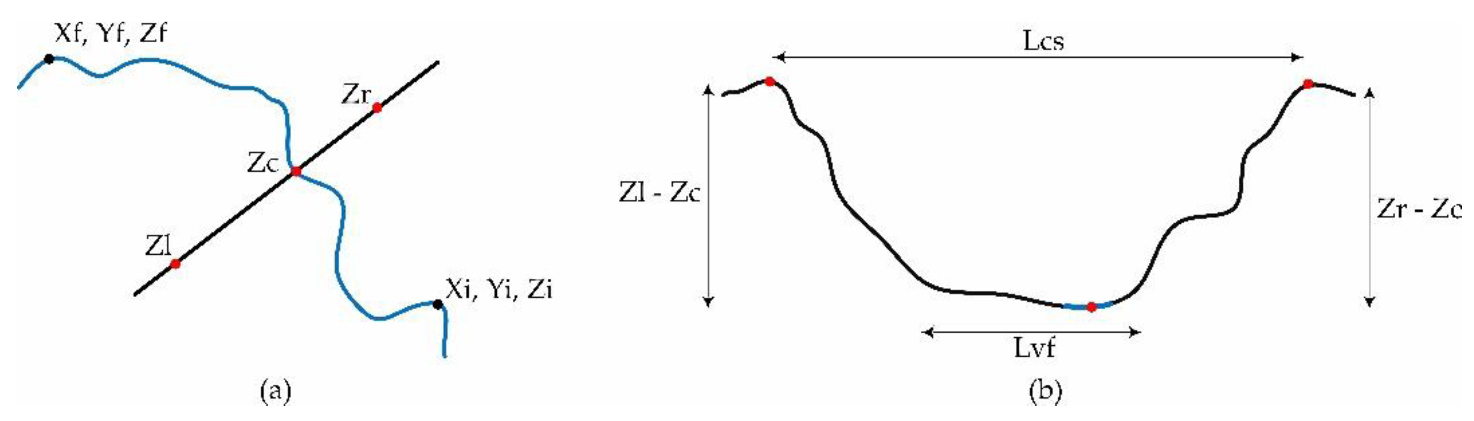
2.7. Geomorphological Classification of Fluvial Systems

The classification of a territory’s fluvial system is an important step in determining its ecological state [55]. The classification of fluvial systems is based on three geomorphological aspects: micro-watershed geomorphology (river style), channel slope, and valley geomorphology (

Table 2. Parameters and geomorphological aspects for river zoning and typification ¹.

Geomorphological Aspects	Geomorphological Parameters	Classification	Range	Symbol
Channel geomorphology	Type of channel	Single channel		N1
		Multiple channels		N2
		Transition		N3
	Sinuosity Index	Straight	<1.05	S1
		Winding	1.05–1.3	S2
		Twisty	1.3–1.5	S3
		Meandering	>1.5	S4
Channel slope	Slope	Level	<0.5%	P1
		Nearly level	0.5–2%	P2
		Gentle slope	2–10%	P3
		Steep	>10%	P4
Valley geomorphology	Confinement	Totally confined	<3	E1
		Very confined	3–12	E2
		Moderately confined	12–22	E3
		Gently confined	22–40	E4
		Unconfined	>40	E5
	Valley bottom width	Null		V1
		Narrow	<50 m	V2
		Medium	50–250 m	V3
		Wide	250–1000 m	V4
		Very Wide	>1000 m	V5

¹ Based on Horacio and Ollero [53], Pardo and Palomar [95].

) [53,54]. The classification process was carried out in two stages allowing fluvial system characterization from a geomorphological perspective: zoning and typification [53]. In regards to zoning, a sectorization of the river system was made for each geomorphological parameter, while with the intersection of these results, the typification stage was carried out. The latter stage involved categorizing, internally and functionally, homogenous types of river channel depending upon geomorphological aspects.

The linear channel layer (.shp) was interpolated with the DEM to acquire the altimetric data of the channel and was divided into sections of 1 km, which is the ideal observation scale for the use of IHG [44]. In the table of attributes, basic descriptors of each section were calculated (Figure 3a): length (L), altitude, and the east and north coordinates of the initial node (Xi, Yi, Zi) and end (Xf, Yf, Zf). Then, over the center of each section, cross sections were drawn with an offset of 750 m on both sides, with the help of the QGIS’s RiverGIS Plugin [94]. These were interpolated with the DEM and the length (Lcs) between the maximum altitude on the left (Zl) and right (Zr) of each cross section was calculated, as well as Zl, Zr, and the central altitude (Zc) corresponding to the channel axis (Figure 3b).

All sections were classified as single channels (N1) (Table 2), due to the infrequency of other channel variants (626 m of 286.50 km). Sinuosity index (S), slope (P), and valley confinement (E) were estimated with the use of Equations (3)–(5) respectively. To calculate valley bottom width (V) through the use of Equation (6), the linear cross-sectional layer (.shp) was imported to the Google Earth Pro interface, where the ruler tool was used to measure said horizontal distance in accordance with each section’s valley morphology as seen in Figure 3b. These data were manually registered to the table of attributes.

S = L/[(Xf − Xi)² + (Yf − Yi)²]^0.5,

(3)

P = [(Zi − Zf)/L] × 100,

(4)

E = Lcs/{[(Zl − Zc) + (Zr − Zc)]/2}

(5)

V = Lvf

(6)

Each morphological parameter was reclassified according to established zoning criteria (Table 2). For the typification process, the fields S, P, E, and V were concatenated for each section. Moreover, adjacent sections with the same classification were grouped. Each group, or Functional Sector (FS), is an internally and functionally homogenous fluvial channel.

2.8. Hydrogeomorphological Quality Evaluation

The hydrogeomorphological quality of each FS of the HAL-MWs was evaluated with the use of the IHG Index [19,46,96]. In the laboratory, hydrological and infrastructure documentation, satellite images (recent and old to assess the change processes; Figure 4), and cartography (terrain topography, land use and road network) were acquired to distinguish pressures and impacts on the river system that may distance its functionality, continuity, naturalness, complexity, and dynamics from a reference state [44]. A hydrogeomorphological process and impact cartographic base was generated [47]. In the field, the channel margins of almost all evaluated kilometers were traveled, during July and August 2017, to apply the final IHG through observations of the current state of the river system. This stage allowed the confirmation of observations in the laboratory, resolving doubts, looking for symptoms of impacts, finding others not visible in images or maps, and combining the expected effects of the these. FSs with difficult access were evaluated only in the laboratory.

The IHG was used to assess three sections of a fluvial system: (1) Functional Quality (FQ), (2) Channel Quality (CQ), and (3) Riparian Quality (RQ), with three subsections each. A score of 10 points was assigned to each subsection. However, these points were subtracted when impacts and damage were observed in accordance with every subsection criterion in the IHG Index. Final hydromorphological quality is calculated according to each FS’ final score in conformity with

Table 3. Total and partial scores for each section (Functional Quality (FQ), Channel Quality (CQ), and Riparian Quality (RQ)) of the Hydrogeomorphological Index (IHG) index and hydrogeomorphological quality classes.

Functional Quality (FQ)	Channel Quality (CQ)	Riparian Quality (RQ)	IHG Index	Hydrogeomorphological Quality
0–6	0–6	0–6	0–20	Very bad
7–13	7–13	7–13	21–41	Poor
14–19	14–19	14–19	42–59	Moderate
20–24	20–24	20–24	60–74	Good
25–30	25–30	25–30	75–90	Very good

[46].

3. Results and Discussion

3.1. Morphometry and Preliminary Priority Ranges (PPR) of the Micro-Watersheds

The HAL-MWs are located at 2198–4275 m.a.s.l in Leimebamba and 1954–3790 m.a.s.l. in Molinopampa (Figure 5). According to Strahler [80], the maximum stream order is three (3).

The morphometric characterizations of HAL-MWs, based on linear variables, area, and shape are reported in

Table 4. Linear, areal, and shape variables of the four HAL-MWs in Leimebamba and two HAL-MWs in Molinopampa (Amazonas, Peru).

Variables		Leimebamba				Molinopampa
		Atuen	Cabildo	Pomacochas	Timbambo	San Antonio	Ventilla
Linear variables
Hmax (m.a.s.l.)		4165	4275	3793	4085	3715	3790
Hmin (m.a.s.l.)		2422	3205	2198	3022	1954	2015
P (km)		44.669	32.753	34.159	28.350	76.506	87.367
A (km2)		48.745	42.967	52.034	23.943	149.785	232.267
Stream order, u	1	5	7	11	5	9	26
	2	1	2	3	1	2	6
	3	2	0	1	0	1	3
Nu	u	8	9	15	6	12	35
Lu (km)		26.792	16.623	36.165	16.715	58.238	131.967
Lsm (km)		3.349	1.847	2.411	2.786	4.853	3.770
L (km)		17.340	7.299	13.087	11.235	27.684	38.113
Sl (%)		4.516	9.248	9.674	7.058	5.375	3.655
Lb (km)		11.931	11.106	12.382	7.967	22.574	28.961
Rb		2.750	3.500	3.333	5.000	3.250	3.167
Areal Variables
Sb (%)		56.298	44.476	41.281	39.391	30.097	31.017
Dd (km/km2)		0.550	0.387	0.695	0.698	0.389	0.568
Fs (km−2)		0.164	0.209	0.288	0.251	0.080	0.151
Rt (km−1)		0.179	0.275	0.439	0.212	0.157	0.401
Lom (km)		0.910	1.292	0.719	0.716	1.286	0.880
Shape Variables
Ff		0.342	0.348	0.339	0.377	0.294	0.277
Rc		0.307	0.503	0.560	0.374	0.322	0.382
Cc		1.805	1.410	1.336	1.634	1.763	1.617
Re		0.660	0.666	0.657	0.693	0.612	0.594

. The results show Rb values ranging from 2.750 (Atuen HAL-WS) to 5.00 (Timbambo HAL-MW). Higher values of Rb indicate greater soil erosion [84]. Dd indicates the closeness of spacing of channels [61], which varies between 0.387 (Cabildo HAL-MW) and 0.698 (Timbambo HAL-MW). Low Dd values occur in regions with dense vegetation, low relief, and highly resistant and permeable subsoils, while high Dd are found in regions with sparse vegetation, high relief, and weak and impermeable subsoils [80]. Melton [97] analyzed the direct relationship between Dd, Fs, and the runoff processes. The high Fs value of the HAL-MW in Pomacochas (0.288) indicates there is more runoff in comparison to other HAL-MWs. Rt is classified into five kinds of texture, ranging from very thick (<2), thick (2–4), moderate (4–6), and good (6–8), to very fine (>8) [98]. All evaluated HAL-MWs show Rt < 2. Lom is an important independent variable that affects the hydrological and physiographic developments of the drainage basin [81]. The shortest Lom, in Timbambo’s HAL-MW (0.716), indicates a faster runoff process than in other HAL-MWs. Ff values > 0.78 indicate circular basins, while lower values indicate elongated basins [99]. Every evaluated HAL-MW has a Ff result of < 0.377. Rc values range between 0.2 and 0.8. Higher results (>0.5), indicate circular basins and homogenous geological material, while lower results (<0.5) indicate elongated basins [86]. Only Cabildo HAL-MW (0.503) and Pomacochas HAL-MW (0.560) have higher Rc values (>0.5). In the case of Cc results, these range from 1.336 (Pomacochas HAL-MW) to 1.805 (Atuen-HAL-MW). Low values of Cc indicate less erosion vulnerability, while higher Cc values indicate a greater erosion risk or vulnerability and the need to implement conservation measures [81]. Regarding Re results, these vary from 0.594 (Ventilla HAL-MW) to 0.693 (Timbambo HAL-MW). Re values close to 1.0 indicate very low relief regions, while 0.4 to 0.8 values indicate very high relief regions and steep slopes [61,65].

After morphometric analysis, PPRs were assigned to all six HAL-MWs (according to the concept of direct and inverse relationships), as indicated in

Table 5. Preliminary Priority Rank (PPR) based on linear, areal, and shape variables of the four HAL-MWs in Leimebamba and two HAL-MWs in Molinopampa (Amazonas, Peru).

Variables	Leimebamba				Molinopampa
	Atuen	Cabildo	Pomacochas	Timbambo	San Antonio	Ventilla
Rb	6	2	3	1	4	5
Dd	4	6	2	1	5	3
Fs	4	3	1	2	6	5
Rt	5	3	1	4	6	2
Lom	3	1	5	6	2	4
Ff	4	5	3	6	2	1
Rc	1	5	6	3	2	4
Cc	6	2	1	4	5	3
Re	4	5	3	6	2	1

.

3.2. Micro-Watershed Prioritization using PCWSA

The positive correlations between the linear morphometric, areal, and shape variables are shown in

Table 6. Correlation matrix between linear, areal, and shape morphometric variables of the four HAL-MWs in Leimebamba and two HAL-MWs in Molinopampa (Amazonas, Peru).

Variables	Rb	Dd	Fs	Rt	Lom	Ff	Rc	Cc	Re
Rb	1.000	0.432	0.465	−0.136	−0.338	0.603 *	0.075	−0.144	0.587
Dd		1.000	0.718 *	0.437	−0.988 ***	0.397	0.212	−0.218	0.386
Fs			1.000	0.515	−0.650 *	0.708 *	0.730 *	−0.732 *	0.706 *
Rt				1.000	−0.439	−0.231	0.727 *	−0.742 *	−0.232
Lom					1.000	−0.324	−0.133	0.139	−0.314
Ff						1.000	0.252	−0.246	0.999 ***
Rc							1.000	−0.993 ***	0.259
Cc								1.000	−0.250
Re									1.000

*** Strong correlation (r > 0.90); ** Good correlation (0.90 ≥ r > 0.75); * Moderate correlation (0.75 ≥ r > 0.60).

. A strong correlation (r > 0.9) is observed between Dd–Lom, Ff–Re, and Rc–Cc, and moderate correlations (r > 0.60) exist between Rb–Ff, Fs–Dd, Fs–Lom, Fs–Ff, Fs–Rc, Fs–Cc, Fs–Re, Rt–Rc, and Rt–Cc.

Table 7. Total variance shown for four HAL-MWs in Leimebamba and two HAL-MWs in Molinopampa (Amazonas, Peru).

Variables	Initial Eigen Value			Extraction Sums of Squared Loadings			Rotation Sums of Squared Loadings
	Total	% of Variance	Cumulative %	Total	% of Variance	Cumulative %	Total	% of Variance	Cumulative %
Rb	4.538	50.424	50.424	4.538	50.424	50.424	3.044	33.817	33.817
Dd	2.407	26.743	77.166	2.407	26.743	77.166	3.012	33.466	67.283
Fs	1.510	16.783	93.949	1.510	16.783	93.949	2.400	26.666	93.949
Rt	0.517	5.742	99.691
Lom	0.028	0.309	100.000
Ff	2.354 × 10−16	2.615 × 10−15	100.000
Rc	−1.559 × 10−17	−1.732 × 10−16	100.000
Cc	−3.626 × 10−17	−4.029 × 10−16	100.000
Re	−9.133 × 10−17	−1.015 × 10−15	100.000

indicates that the top three components have values >1.5, and together, these represent about 93.949% of the total variance. However, at this stage, it was too difficult to classify the variables into components and add physical significance [65].

Therefore, the first FL (not rotated) and the rotated FL were constructed using principal component analysis (

Table 8. Unrotated and rotated factor-loading matrix of morphometric variables.

Variables	Principal Component—Unrotated			Principal Component—Rotated (VARIMAX)
	1	2	3	1	2	3
Rb	0.549	0.534	0.033	−0.035	0.715 *	0.275
Dd	0.762 **	0.098	−0.634 *	0.148	0.272	0.947 ***
Fs	0.993 ***	−0.043	0.056	0.647 *	0.576	0.490
Rt	0.499	−0.825 **	−0.232	0.794 **	−0.381	0.458
Lom	−0.690 *	−0.080	0.713 *	−0.087	−0.186	−0.974 ***
Ff	0.703 *	0.607 *	0.318	0.113	0.968 ***	0.120
Rc	0.688 *	−0.592	0.412	0.986 ***	0.146	0.021
Cc	−0.698 *	0.585	−0.402	−0.983 ***	−0.153	−0.035
Re	0.699 *	0.601 *	0.329	0.120	0.966 ***	0.108

*** Strong correlation (r > 0.90); ** Good correlation (0.90 ≥ r > 0.75); * Moderate correlation (0.75 ≥ r > 0.60).

). Due to the fact that the third component (PC–3) of the first FL is moderately correlated with Dd and Lom, it is difficult to obtain a physically important component [65]. However, after analyzing the rotated FL matrix, the most important morphometric variables were Lom (PC–3), Ff (PC–2), and Rc (PC–1). This is in contrast to research done by Malik et al. [65], who, while using the same nine morphometric variables, found that the most important variables for nine sub basins in the Bino basin of India were Fs, Lom, and Ff.

Cross-correlation between the three significant morphometric variables (Lom, Ff, and Rc) is shown in

Table 9. Cross-correlation matrix of the Lom, Ff, and Rc variables of four HAL-MWs in Leimebamba and two HAL-MWs in Molinopampa (Amazonas, Peru).

Variables	Lom	Ff	Rc
Lom	1.000	−0.324	−0.133
Ff	−0.324	1.000	0.252
Rc	−0.133	0.252	1.000
Sum of correlation	0.543	0.928	1.119
Grand total	2.590	2.590	2.590
Weight	0.209	0.358	0.432

, while CF values and the final priority range are indicated in

Table 10. Final priority rank based on the Composite Factor (CF) value of the four HAL-MWs in Leimebamba and two HAL-MWs in Molinopampa (Amazonas, Peru).

	Leimebamba				Molinopampa
	Atuen	Cabildo	Pomacochas	Timbambo	San Antonio	Ventilla
Composite Factor (CF)	2.491	4.159	4.711	4.698	1.998	2.922
Priority Rank	2	4	6	5	1	3

. From the six evaluated HAL-MWs, the established priority for the San Antonio HAL-MW is 1 and the Pomacochas HAL-MW has a priority of 6.

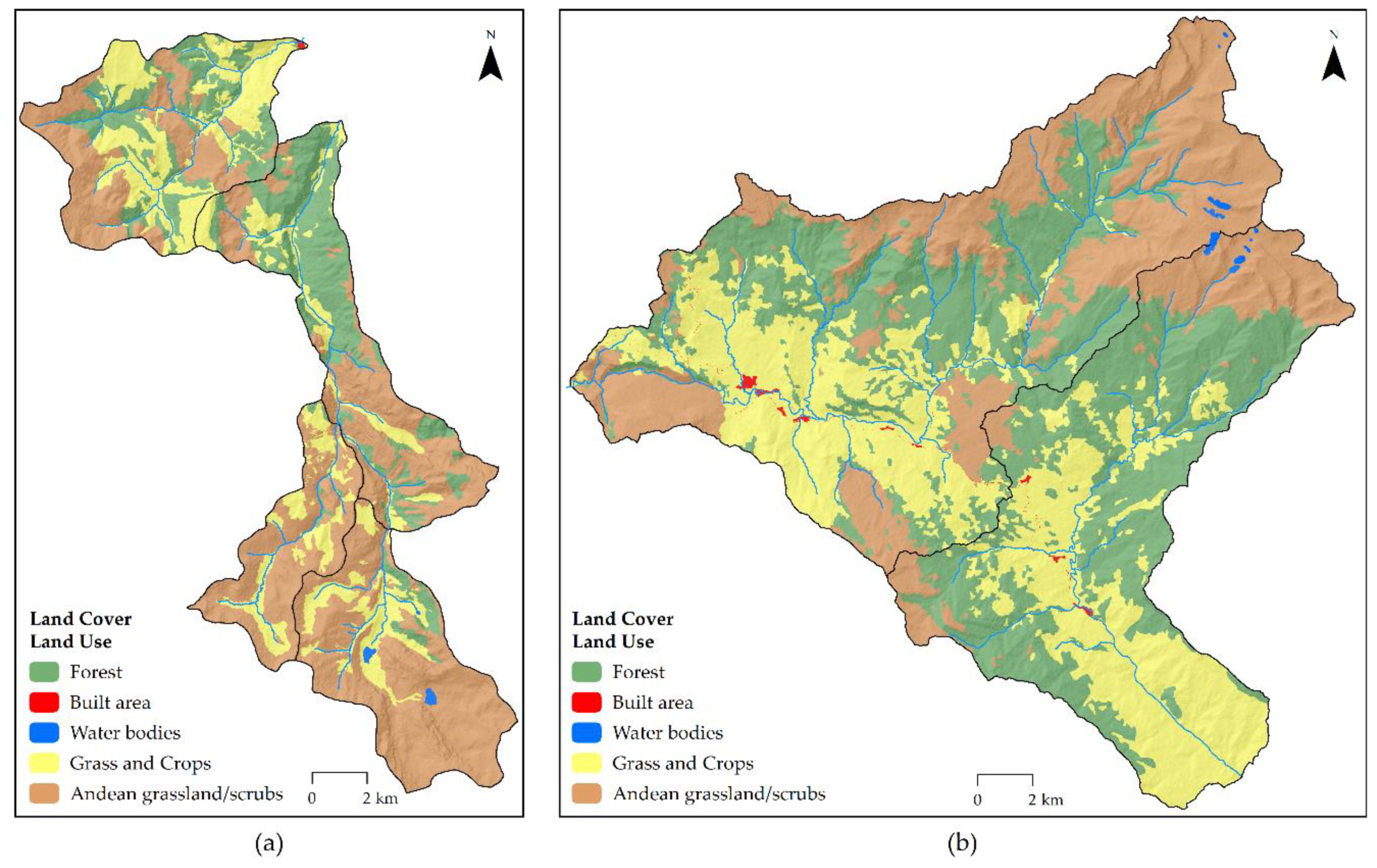
3.3. Land Cover/Land Use (LC/LU)

Figure 6 depicts the LC/LU spatial distribution pattern for the HAL-MWs in 2017. The general accuracies of the classifications for the LC/LU maps for the Leimebamba and Molinopampa MWs were 0.90 and 0.93. The calculated kappa coefficient (k) for Leimebamba (k = 0.84) and Molinopampa (k = 0.90) indicates an “Almost Perfect” map–terrain agreement [100]. After a supervised classification, visual interpretation allowed us to correct errors generated by the spectral similarity between the “GC” and “AG/S” types of grass. This is a direct consequence of the frequent transitions and overlapping of the types of grass [24].

Natural land coverage (“Fo” plus “AG/S”) constitutes 62.3% to 84.4% of the territory of each HAL-MW, as well as 75.2% and 69.0% of the territory evaluated in Leimebamba and Molinopampa, respectively (

Table 11. Land Cover/Land Use (LC/LU) of the four HAL-MWs in Leimebamba and two HAL-MWs in Molinopampa (Amazonas, Peru).

LC/LU	Leimebamba										Molinopampa
	Atuen		Cabildo		Pomacochas		Timbambo		Total		San Antonio		Ventilla		Total
	km2	%	km2	%	km2	%	km2	%	km2	%	km2	%	km2	%	km2	%
Fo	20.69	42.4	2.10	4.9	13.56	26.1	0.50	2.1	36.85	22.0	69.74	46.6	72.57	31.2	142.31	37.2
AG/S	20.46	42.0	32.85	76.4	19.03	36.6	16.95	70.8	89.29	53.2	23.54	15.7	97.65	42.0	121.19	31.7
GC	7.60	15.6	7.62	17.7	19.37	37.2	6.50	27.1	41.08	24.5	56.02	37.4	61.15	26.3	117.17	30.7
WB	–	–	0.40	0.9	–	–	–	–	0.40	0.2	0.22	0.1	0.13	0.1	0.36	0.1
BA	–	–	–	–	0.07	0.1	–	–	0.07	0.0	0.27	0.2	0.77	0.3	1.03	0.3
Total	48.75	100.0	42.97	100.0	52.03	100.0	23.94	100.0	167.69	100.0	149.79	100.0	232.27	100.0	382.06	100.0

). The largest areas of “BA” (0.77 km²) and “GC” (61.15 km²) are found in the Ventilla HAL-MW. Agricultural and livestock activities are present throughout all HAL-MWs and present the greatest anthropic pressure on soil and water. Oliva et al. [31] evaluated four different productive systems in Molinopampa: forest (PS1), open field pasture (PS2), a silvopasture system with Pinus patula (PS3), and another with Alnus acuminata (PS4). Of these, PS2 recorded the highest soil compaction value (395 psi), apparent density (0.93 g/cm³), and EC (0.36 μS/cm), as well as the lowest values of phosphorus (4.22 ppm), organic carbon (3.64%), organic matter (5.92%), and nitrogen (0.31 ppm). According to both this research and another investigation [30], pH levels tend to decrease in the high Andean Pinus patula plantations of Amazonas because they are closely linked to plantation age and vegetation density. In the San Antonio HAL-WS, Oliva et al. [29] studied seven stages of migratory agriculture and observed that this process generates significant changes in physiochemical soil characteristics at different depths (greater impact at 0–15 cm than at 15–30 cm) due to forest-cutting and burning practices.

The “AG/S” type is the most representative (53.2%) amongst the HAL-MWs in Leimebamba, followed by “GC” (24.5%) and “Fo” (22.0 %). Ramírez [67], Salas et al. [25], and Rojas et al. [24] report that “AG/S ‘s” natural meadows in Amazonas are used as natural open field pastures and managed by periodic anthropic burning. Furthermore, Vasquez et al. [28] recorded 129 weed species (out of 148 herbaceous plants) in these natural grasslands. The average abundance and the number of weed species in PS2 and silvopastures (PS3, PS4, and others) were 41.32% and 22.07%, and 111 and 70, respectively. Mendoza et al. [27] found that between 1989 and 2016, 32.02 km² of forest were lost in Leimebamba, at a rate of 1.19 km²/year, attributed to agricultural and livestock pasture expansion (“GC”). In the case of the Molinopampa HAL-MW, the “Fo” type is the most representative with 37.2%. In the specific case of the San Antonio HAL-MW, García-Pérez et al. [23] characterized the local homogeneous palm forest (genus Ceroxylon) and indicated that the low diversity of species (C. peruvianum, C. quindiuense, C. vogelianum, and C. parvifrons) is due to interaction with activities such as agriculture and livestock. However, Sanín [101] explains that a similar density of adult C. quindiuense in deforested grasslands and in forests may be due to (i) adult palm trees being saved from logging and (ii) regeneration through underground meristems after pasture installation.

Bacteriological parameters were analyzed in the most dynamic river areas of “GC” and “BC” types of HAL-MW in Ventilla (Figure 4b) by Chávez et al. [33], and indicated that this area is considerably contaminated by the presence of cattle near riverbanks and city wastewater discharge. Studies of macroinvertebrates, and the physicochemical and microbiological properties of water in other HAL-MWs of Amazonas, such as Alto Imaza [32], El Chido and Allpachaca–Lindapa [34], Chinata, and Gocta [36] and Shocol [35], show that quality decreases as a consequence of anthropic pressure in “GC”, and “BA”. Lastly, Ibisate et al. [47] indicate that the loss of hydrogeomorphological quality is closely linked to the sociodemographic pressure caused by the proliferation of artificial uses in the channel and the flood plain, but also by changes in basin land uses.

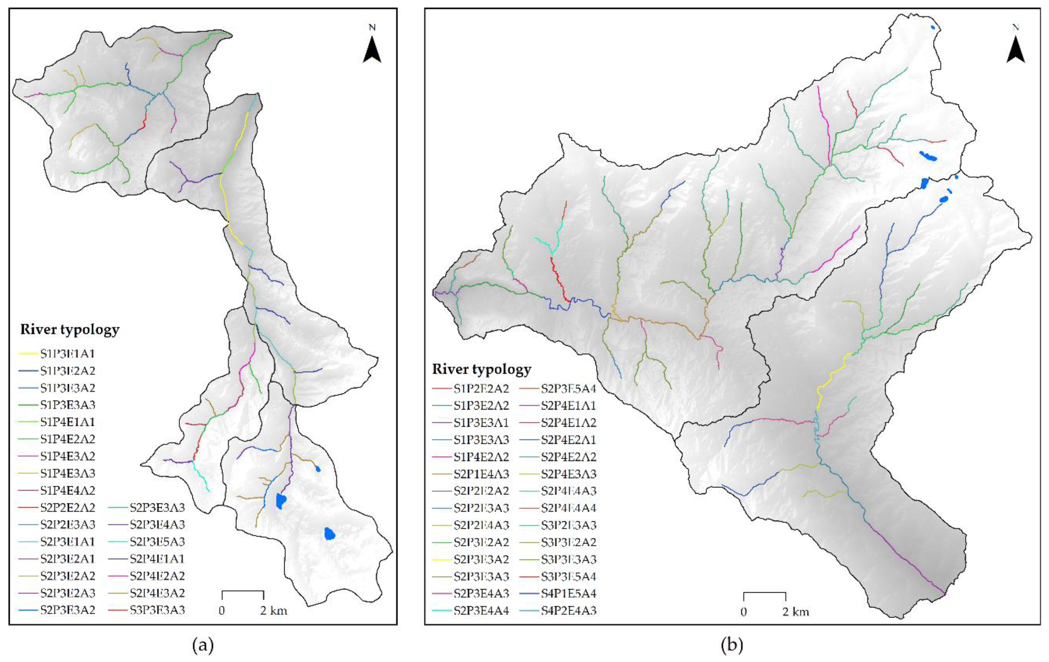
3.4. Fluvial Typology and Functional Sectors (FS)

Twenty-three types of river typology were identified in the Leimebamba HAL-MWs as a result of the combination of nine types of valley and six types of riverbed characterized in the fluvial typification stage (Figure 7a;

Table 12. Percentages (%) of occupancy of types of riverbed and valley of the four HAL-MWs in Leimebamba (Amazonas, Peru).

		Valley Geomorphology									Total
		E1V1	E2V2	E3V2	E3V3	E4V2	E2V1	E2V3	E4V3	E5V3
Channel Geomorphology	S1P3	5.99	2.36	1.17	7.21	–	–	–	–	–	16.73
	S1P4	1.33	12.74	3.70	6.63	1.07	–	–	–	–	25.47
	S2P2	–	1.05	–	4.39	–	–	–	–	–	5.44
	S2P3	6.33	5.26	3.37	2.14	–	2.17	2.14	8.99	2.14	32.54
	S2P4	6.79	2.14	8.74	–	–	–	–	–	–	17.68
	S3P3	–	–	–	2.14	–	–	–	–	–	2.14
Total		20.44	23.55	16.98	22.52	1.07	2.17	2.14	8.99	2.14	100.00

). Twenty-eight river typologies were identified in Molinopampa from 10 types of valley and nine types of riverbed (Figure 7b;

Table 13. Percentages (%) of occupancy of types of riverbed and valley in the two HAL-MWs in Molinopampa (Amazonas, Peru).

		Valley Geomorphology										Total
		E2V2	E3V1	E3V3	E4V3	E3V2	E4V4	E5V4	E1V1	E1V2	E2V1
Channel Geomorphology	S1P2	0.53	–	–	–	–	–	–	–	–	–	0.53
	S1P3	6.40	2.70	0.60	–	–	–	–	–	–	–	9.70
	S1P4	3.89	–	–	–	–	–	–	–	–	–	3.89
	S2P1	–	–	–	4.22	–	–	–	–	–	–	4.22
	S2P2	2.18	–	5.16	1.08	–	–	–	–	–	–	8.42
	S2P3	5.00	–	12.80	4.77	2.16	1.80	0.75	–	–	–	27.27
	S2P4	17.81	–	4.39	0.56	–	0.55	–	0.59	1.66	8.14	33.70
	S3P2	–	–	3.34	–	–	–	–	–	–	–	3.34
	S3P3	1.62	–	1.11	–	–	–	1.64	–	–	–	4.36
	S4P1	–	–	–	–	–	–	2.94	–	–	–	2.94
	S4P2	–	–	–	1.62	–	–	–	–	–	–	1.62
Total		37.43	2.70	27.40	12.24	2.16	2.34	5.33	0.59	1.66	8.14	100.00

). In sum, 39 river typologies were identified from a combination of 13 types of valley and 11 types of riverbed. This figure reflects a very high landscape and river diversity.

Table 12 and Table 13 indicate the occupancy percentages of each type of riverbed and valley. The dominant river typology in Leimebamba is a high slope straight channel located in a very tight valley and narrow river bottom (S1P4–E2V2) with 12.74%, followed by a moderately high sloped winding channel located in a gently fitted valley with a medium width river bottom (S2P3–E4V3; 8.99%), and finally by a high sloped winding channel located in a moderately fitted valley with a narrow width river bottom (S2P4–E3V2; 8.74%). In conclusion, sinuous riverbends with moderately high slopes (S2P3; 32.54%) and fitted valleys with wide width river bottoms (E2V2; 23.55%) are predominant.

In Molinopampa, the dominant typology, with 17.81%, is rivers with sinuous high slopes located in a very tight valley with a narrow river bottom (S2P4–E2V2), followed by winding channel rivers with moderately high slopes in moderately fitted valleys and medium-width river bottoms (S2P3–E3V3; 12.80%), and finally by straight channel rivers with moderately-high slopes in very tight valleys with narrow river bottoms (S1P3–E2V2; 8.74%). In general, sinuous rivers with high slopes (S2P4; 33.70%) located in very embedded valleys with narrow river bottoms are predominant (E2V2; 37.43%).

Ollero [52] stated that river geodiversity is one of the planet’s richest natural heritage features and therefore classifying channels and valleys is fundamental for any river study. Even though the most recent geomorphological methodology [53,54,55,56,57] is based on lithological units at a 1:50,000 scale and topographic units are generated with a 5 m spatial resolution DEM (Lithotopo) [57], this approach was not applied for the present study. Regardless of the fact that topographic units (altitude, slope, and roughness) can be generated from the most detailed DEM available in Peru (ALOS PALSAR, 12.5 m), the National Geological Cuadrangle lithology is not yet available at a 1:50,000 scale for the entire Peruvian territory. In addition, this computing resource is not useful for detailed local scale (micro-basins and stretches <1 km) work.

In Leimebamba and Molinopampa, 53 FS and 65 FS were assembled within 48.96 km and 65.80 km of total channel length, respectively (

Table 14. Number of Functional Sectors (FS) of the four HAL-MWs in Leimebamba and two HAL-MWs in Molinopampa (Amazonas, Peru).

Leimebamba					Molinopampa			Grand Total
Atuen	Cabildo	Pomacochas	Timbambo	Total	San Antonio	Ventilla	Total
12	12	19	10	53	17	48	65	118

). These had variable lengths, from 0.30 km (FS4 in Cabildo HAL-MW) to 8.02 km (FS25 in Ventilla HAL-MW). Ollero et al. [44] mention that the smaller the FS (greater detailed work), the more accurate the resulting evaluation. However, they also state that the level of detail is conditioned by the study objective, or even by the budget itself. For example, Barboza et al. in the Utcubamba basin [37] and in the Leiva MW [38] considered eight FS and 17 FS in 250 km and 56.48 km of the total channel, respectively.

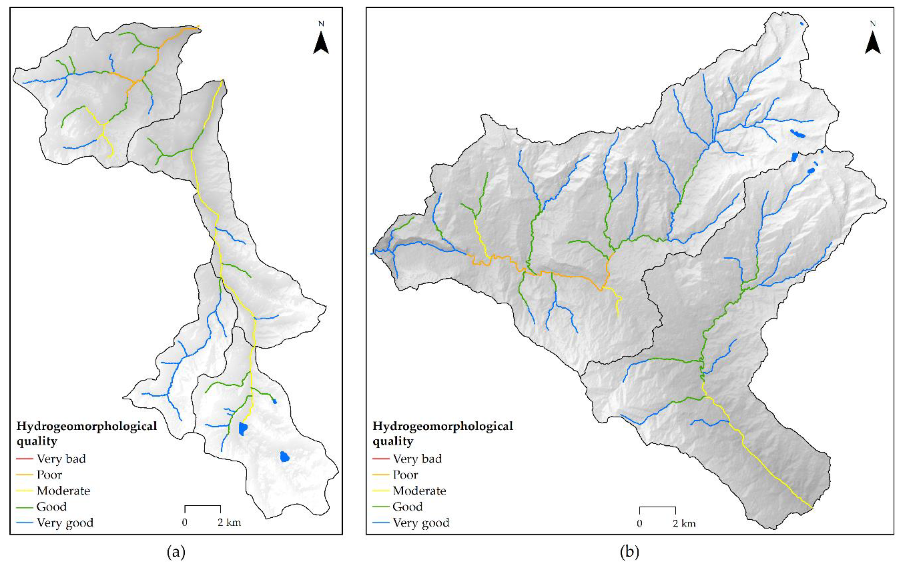
3.5. Hydromorphological Quality Determination using IHG

Figure 8 shows the hydrogeomorphological quality pattern of the channels in all six HAL-MWs. In general, a deterioration in quality is observed as the altitude descends, from the high channels (tributaries of order 1) to the medium and low channels, except in the Ventilla HAL-MW. This pattern was found by Barboza et al. [37] in the Utcubamba basin.

In Leimebamba, the total IHG assessment showed that 8.5%, 26.6%, 30.5%, and 34.4% of the lengths of the channels are assessed as being of “Poor”, “Moderate”, “Good”, and “Very good” quality, respectively (

Table 15. Hydrogeomorphological quality (IHG) assessments of the four HAL-MWs in Leimebamba and two HAL-MWs in Molinopampa (Amazonas, Peru).

Quality	Leimebamba										Molinopampa
	Atuen		Cabildo		Pomacochas		Timbambo		Total		San Antonio		Ventilla		Total
	km	%	km	%	km	%	km	%	km	%	km	%	km	%	km	%
Functional quality
Very bad	–	–	–	–	–	–	–	–	–	–	–	–	–	–	–	–
Poor	–	–	–	–	4.21	11.7	–	–	4.21	4.4	–	–	13.61	10.3	13.61	7.2
Moderate	8.93	33.3	1.15	6.9	8.84	24.4	–	–	18.91	19.6	10.25	17.6	3.11	2.4	13.36	7.0
Good	9.06	33.8	7.61	45.8	5.64	15.6	–	–	22.31	23.2	15.64	26.9	25.99	19.7	41.63	21.9
Very good	8.81	32.9	7.87	47.3	17.48	48.3	16.72	100.0	50.86	52.8	32.34	55.5	89.26	67.6	121.61	63.9
Channel quality
Very bad	–	–	–	–	–	–	–	–	–	–	–	–	–	–	–	–
Poor	–	–	–	–	–	–	–	–	–	–	–	–	–	–	–	–
Moderate	10.20	38.1	2.09	12.5	13.05	36.1	–	–	25.34	26.3	–	–	16.72	12.7	16.72	8.8
Good	13.01	48.6	9.84	59.2	11.60	32.1	–	–	34.45	35.8	13.33	22.9	13.34	10.1	26.67	14.0
Very good	3.58	13.4	4.70	28.3	11.51	31.8	16.72	100.0	36.51	37.9	44.91	77.1	101.91	77.2	146.82	77.2
Riparian quality
Very bad	–	–	–	–	–	–	–	–	–	–	–	–	–	–	–	–
Poor	–	–	–	–	4.03	11.1	–	–	4.03	4.2	–	–	13.61	10.3	13.61	7.2
Moderate	1.27	4.8	5.97	35.9	4.21	11.7	–	–	11.45	11.9	16.57	28.5	8.28	6.3	24.86	13.1
Good	21.94	81.9	7.10	42.7	17.74	49.1	8.835	52.9	55.62	57.8	14.91	25.6	30.05	22.8	44.96	23.6
Very good	3.58	13.4	3.55	21.4	10.18	28.2	7.88	47.1	25.19	26.2	26.75	45.9	80.02	60.6	106.78	56.1
Hydrogeomorphological quality (IHG index)
Very bad	–	–	–	–	–	–	–	–	–	–	–	–	–	–	–	–
Poor	–	–	–	–	8.14	22.5	–	–	8.14	8.5	–	–	13.61	10.3	13.61	7.2
Moderate	15.94	59.5	4.84	29.1	4.81	13.3	–	–	25.60	26.6	10.25	17.6	5.74	4.4	15.99	8.4
Good	7.27	27.1	8.18	49.2	12.99	35.9	0.97	5.8	29.41	30.5	17.88	30.7	32.69	24.8	50.57	26.6
Very good	3.58	13.4	3.59	21.6	10.22	28.3	15.75	94.2	33.14	34.4	30.11	51.7	79.92	60.6	110.03	57.8
Total	26.79	100.0	16.62	100.0	36.17	100.0	16.72	100.0	96.29	100.0	58.24	100.0	131.97	100.0	190.21	100.0

). In Molinopampa, 7.2%, 8.4%, 26.6%, and 57.8% of the lengths of the channels have “Poor”, “Moderate”, “Good”, and “Very good” quality assessments. None of the sections of the six assessed HAL-MWs had a “Very bad” quality. Hence, sections that were assessed as “Good” and “Very good” can be considered as reference sections for river restoration [47].

In the high channels of Leimebamba and Molinopampa, the riverbank and floodplain degradation is predominantly caused by pressure from livestock and agricultural activities, such as grazing, migratory agriculture, clearing, fires, etc., that alter soil structure [18,22], induce shrubland growth due to the disconnection with the phreatic zone [10], stimulate weed proliferation [28], and produce longitudinal discontinuities [37]. The most important immediate impacts registered are those derived from vehicular and pedestrian bridges, small weirs, channels, and longitudinal stone defenses. Dams, canals, irrigation systems, and other hydraulic works cause deterioration in the river current, which often has irreversible and sometimes unknown consequences [11,48]. One exception is the Timbambo HAL-MW, where aggregate extraction is non-existent due to its road inaccessibility. This particular activity (aggregate extraction), when done massively and indiscriminately, causes lateral river incision and tends to affect riverbank and riverbed natural sediment accumulation areas [8]. Furthermore, the extensive access roads to crop parcels and access trails to basins for cattle break transversal riverbank connectivity are noteworthy [44]. The gravel surface of the Leimebamba–Chuquibamba road that runs parallel to, and sometimes intersects, the Cabildo and Atuen HAL-MWs, alters their hydromorphological processes causing overflows, floods, and flood flows [44]. The same impacts on San Antonio and Ventilla HAL-MWs are caused by the asphalt-covered road that connects Chachapoyas and Mendoza. Irrespective of the negative impacts just described, road infrastructure favors livestock growth and small-scale agricultural migration [24]. The case of the Pomacochas HAL-MW differs as it is located near the final road section and the district capital of Leimebamba (Figure 4a). Along this urban section, the floodplain has disappeared, the margins have been completely channeled, there are abundant obstacles, and the entire floodplain has been raised or waterproofed. In the Timbambo HAL-MW, 5.8% and 94.2% of the lengths of the channels have “Good” and “Very good” quality assessments, and this therefore has the largest number of sections that can be considered as reference conditions for river restoration [47].

Finally, it can be concluded that hydrogeomorphological river alterations originate because of socio-economical activities that consume water, sediments (“aggregates”), and territory (river space), and also due to community preferences for living next to rivers in risky situations that require infrastructural protection against floods and river dynamics [8].

3.6. Morphometric Prioritization, Fluvial Classification, and Hydrogeomorphological Quality

Watershed prioritization examines the intensity of each HAL-MW’s erosion problem so that the range will be used to prioritize the treatment of each with soil and water conservation measures [65]. River and valley geomorphological classification is fundamental for any kind of fluvial study. Hence, it must be used in any land planning project as an essential reference instrument for the understanding, functioning, and enhancement of natural systems [53]. Hydrogeomorphological dynamics guarantee the protection of each and every one of the elements of the river system, and it is the key not only to its functioning but also to its ecological, landscape, and environmental value [19]. Various studies of morphometric prioritization utilizing multivariate statistics [58,61,62,63,64,65], geomorphological river classifications [53,54,55,56,57], and evaluations of hydrogeomorphological quality using IHG have been carried out [37,38,44,45,47,48,49]. From the aforementioned, two did not integrate fluvial classification prior to the use of the IHG [48,49]. However, the integration of the three different methodologies used in this study [19,53,65] has not yet been reported.

This study evaluated the feasibility of an integrated approach to morphometric prioritization, geomorphological river classification, and the hydrogeomorphological assessment of micro-watersheds. The proposed methodology allows us to identify and prioritize micro-watersheds susceptible to erosion and riverbed sections in need of conservation and/or restoration to inform and improve the decision-making process in the selected study area. However, future research could incorporate ecological, socioeconomic, and geospatial perspectives to further enhance this kind of modeling.

4. Conclusions

The PCWSA hybrid model reveals that the San Antonio HAL-MW and the Atuen HAL-MW are located in areas very susceptible to erosion. Therefore, they were assigned top priorities, and rapid soil adaptation and water conservation practices are recommended. Consequently, the priority order is as follows: Ventilla HAL-MW, Cabildo HAL-MW, Timbambo HAL-MW, and Pomacochas HAL-MW. Concerning geomorphological river classification, 39 types of river course were identified within the six HAL-MWs, as the result of combining 13 types of valley and 11 types of riverbed, thereby indicating very high landscape and river diversity. Total IHG assessment gave results of 7.6% (21.8 km), 14.5% (41.6 km), 27.9% (80.0 km), and 50.0% (143.2 km) of the total channel lengths being of a “Poor”, “Moderate”, “Good”, and “Very good” quality, respectively. None of the sections of the six assessed HAL-MWs had a “Very bad” quality assessment, hence sections that were assessed as “Good” and “Very good” can be considered as reference sections for river restoration. The loss of hydrogeomorphological quality is closely linked to the sociodemographic pressures caused by the rise in anthropic modifications of the basin and floodplain.

Given the importance of the HAL-MW ecosystems in Amazonas and in Peru, an integrated methodological framework of morphometric prioritization, geomorphological river classification, and hydrogeomorphological evaluation of hydrographic micro-watersheds is presented. Ergo, due to its low complexity, this methodology can be replicated, with the use of necessary complements, in all Peruvian ecosystems and will ultimately contribute to adequate territory, soil, and water planning and management.

References

1. FAO. El Estado de los Recursos de Tierras y aguas del Mundo para la Alimentación y la Agricultura. La Gestión de los Sistemas en Situación de Riesgo; FAO: Roma, Italy, 2012; ISBN 9789253066148. [Google Scholar]
2. ONU. La Situación Demográfica en el Mundo, Informe Conciso; ONU: New York, NY, USA, 2014; pp. 1–38. Available online: https://shop.un.org/books/informe-conciso-sobre-la-situacion-43680 (accessed on 6 May 2020).
3. FAO. Huella de agua de la industria bananera. In Proceedings of the Foro Mundial Bananero; FAO: Roma, Italy, 2017; p. 5. Available online: http://www.fao.org/3/a-i6914s.pdf (accessed on 6 May 2020).
4. PNUMA. Estado del Medio Ambiente en ALC. In Perspectivas del Medio Ambiente: America Latina y El Caribe—GEO ALC 3; PNUMA: Panamá, Panamá, 2010; pp. 59–182. ISBN 9789280729566. [Google Scholar]
5. Guevara, P.E.; De La Torre, V.A.A. La situación de los recursos hídricos en el Perú. In Gestión Integrada de los Recursos Hídricos por Cuenca y Cultura del Agua; Guevara Pérez, E., De La Torre Villanueva, A.A., Eds.; ANA: Lima, Perú, 2019; pp. 715–770. ISBN 9786124273278. [Google Scholar]
6. Kámiche, Z.J. Agua: Buscando Mecanismos para Lograr un Manejo Eficiente del agua. En Agenda 2011; Universidad del Pacífico: Lima, Perú, 2011; pp. 1–4. [Google Scholar]
7. ANA. Política y Estrategia Nacional de Recursos Hídricos; ANA: Lima, Perú, 2015. [Google Scholar]
8. Ballarín Ferrer, D.; Rodríguez Muñoz, I. Hidromorfología Fluvial: Algunos Apuntes Aplicados a la Restauración de Ríos en la Cuenca del Duero; Confederación Hidrográfica del Duero (Ministerio de Agricultura, Alimentación y Medio Ambiente): Valladolid, Spain, 2013. [Google Scholar]
9. Aguiar, F.C.; Ferreira, M.T. Plant invasions in the rivers of the Iberian Peninsula, south-western Europe: A review. Plant Biosyst. Int. J. Deal. All Asp. Plant Biol. 2013, 147, 1107–1119. [Google Scholar] [CrossRef]
10. Lozanovska, I.; Ferreira, M.; Aguiar, F.C. Functional diversity assessment in riparian forests—Multiple approaches and trends: A review. Ecol. Indic. 2018, 95, 781–793. [Google Scholar] [CrossRef]
11. Braatne, J.H.; Rood, S.B.; Goater, L.A.; Blair, C.L. Analyzing the Impacts of Dams on Riparian Ecosystems: A Review of Research Strategies and Their Relevance to the Snake River Through Hells Canyon. Environ. Manag. 2007, 41, 267–281. [Google Scholar] [CrossRef] [PubMed] [Green Version]
12. Atlas Merrill, M. The Effects of Culverts and Bridges on Stream Geomorphology. Master’s Thesis, North Carolina State University, Raleigh, NC, USA, 2005. Available online: https://repository.lib.ncsu.edu/handle/1840.16/1476 (accessed on 6 May 2020).
13. Gregory, K.; Brookes, A. Hydrogeomorphology downstream from bridges. Appl. Geogr. 1983, 3, 145–159. [Google Scholar] [CrossRef]
14. Petts, G.; Gurnell, A. 13.7 Hydrogeomorphic Effects of Reservoirs, Dams, and Diversions. Treatise Geomorphol. 2013, 13, 96–114. [Google Scholar] [CrossRef]
15. Vietz, G.J.; Walsh, C.J.; Fletcher, T.D. Urban hydrogeomorphology and the urban stream syndrome. Prog. Phys. Geogr. Earth Environ. 2015, 40, 480–492. [Google Scholar] [CrossRef]
16. Mossa, J.; James, L.; James, A. 13.6 Impacts of Mining on Geomorphic Systems. Treatise Geomorphol. 2013, 13, 74–95. [Google Scholar] [CrossRef]
17. Roy, S.; Sahu, A.S. Potential interaction between transport and stream networks over the lowland rivers in Eastern India. J. Environ. Manag. 2017, 197, 316–330. [Google Scholar] [CrossRef]
18. Butler, D. Grazing Influences on Geomorphic Systems. Treatise Geomorphol. 2013, 13, 68–73. [Google Scholar] [CrossRef]
19. Ollero, A.O.; Ferrer, D.B.; Bea, E.D.; Mur, D.M.; Fabre, M.S.; Naverac, V.A.; Arnedo, M.T.E.; García, D.G.; De Matauco, A.I.G.; Gil, L.S. Un índice hidrogeomorfológico (IHG) para la evaluación del estado ecológico de sistemas fluviales. Geographicalia 2007, 52, 113–141. [Google Scholar] [CrossRef] [Green Version]
20. Gutiérrez, E.M. Geomorfología Fluvial I. In Geomorfología; Pearson/Prentice Hall: Madrid, Spain, 2008; pp. 275–302. ISBN 9788483223895. [Google Scholar]
21. Elosegi, A.; Sabater, S. Effects of hydromorphological impacts on river ecosystem functioning: A review and suggestions for assessing ecological impacts. Hydrobiologia 2012, 712, 129–143. [Google Scholar] [CrossRef]
22. Royall, D. 13.3 Land-Use Impacts on the Hydrogeomorphology of Small Watersheds. Treatise Geomorphol. 2013, 13, 28–47. [Google Scholar] [CrossRef]
23. García-Pérez, A.; Rubio, R.K.B.; Meléndez, M.J.B.; Corroto, F.; Rascón, J.; Oliva, M. Estudio ecológico de los bosques homogéneos en el distrito de Molinopampa, Región Amazonas. Rev. Investig. Agroproducción Sustentable 2018, 2, 73–79. [Google Scholar]
24. Briceño, N.B.R.; Castillo, E.B.; Maicelo-Quintana, J.; Oliva-Cruz, M.; López, R.S. Deforestación en la Amazonía peruana: Índices de cambios de cobertura y uso del suelo basado en SIG. BAGE 2019, 81, 1–34. [Google Scholar] [CrossRef]
25. Salas, L.R.; Barboza, C.E.; Rojas, B.N.B.; Rodriguez, C.N.Y. Deforestación en el área de conservación privada Tilacancha: Zona de recarga hídrica y de abastecimiento de agua para Chachapoyas. Rev. Investig. Agroproducción Sustentable 2018, 2, 54–64. [Google Scholar]
26. Salas, L.R.; Barboza, C.E.; Oliva, C.M. Dinámica multitemporal de índices de deforestación en el distrito de Florida, departamento de Amazonas, Perú. Revista INDES 2014, 2, 18–27. [Google Scholar]
27. Mendoza, C.M.E.; Salas, L.R.; Barboza, C.E. Análisis multitemporal de la deforestación usando la clasificación basada en objetos, distrito de Leymebamba (Perú). Rev. INDES 2015, 3, 67–76. [Google Scholar] [CrossRef] [Green Version]
28. Vasquez, P.H.; Maicelo, Q.J.L.; Collazos, S.R.; Oliva, C.S.M. Selección, identificación y distribución de malezas (adventicias), en praderas naturales de las principales microcuencas ganaderas de la región Amazonas. Revista INDES 2014, 2, 71–79. [Google Scholar]
29. Oliva, C.S.M.; Maicelo, Q.J.L.; Torres, G.C.; Bardales, E.W. Propiedades fisicoquímicas del suelo en diferentes estadios de la agricultura migratoria en el Área de Conservación Privada “Palmeras de Ocol”, distrito de Molinopampa, provincia de Chachapoyas (departamento de Amazonas). Rev. Investig. Agroproducción Sustentable 2017, 1, 9–21. [Google Scholar]
30. Oliva, C.S.M.; Collazos, S.R.; Espárraga, E.T.A. Efecto de las plantaciones de Pinus patula sobre las características fisicoquímicas de los suelos en áreas altoandinas de la región Amazonas. Revista INDES 2014, 2, 28–36. [Google Scholar]
31. Oliva, C.M.; Collazos, S.R.; Goñas, M.M.; Bacalla, E.; Vigo, M.C.; Vásquez, P.H.; Espinosa, L.S.T.; Maicelo, Q.J.L. Efecto de los sistemas de producción sobre las características físico-químicas de los suelos del distrito de Molinopampa, provincia de Chachapoyas, región Amazonas. Revista INDES 2014, 2, 44–52. [Google Scholar]
32. Corroto, F.; Yalta, M.J.R.; Vásquez, P.H.V.; Gamarra, T.O.A. Evaluación de la calidad ecológica del agua en la cuenca alta del río Imaza (Perú). Revista INDES 2014, 2, 20–29. [Google Scholar]
33. Chávez, O.J.; Rascón, J.; Eneque, P.A. Evaluación del impacto del vertimiento de aguas residuales en la calidad del río Ventilla, Amazonas. Revista INDES 2015, 3, 99–107. [Google Scholar]
34. Gamarra, T.O.A.; Yalta, M.J.R.; Salas, L.R.; Alvarado, C.L.; Oliva, C.S.M. Evaluación de la calidad ecológica del agua en la microcuenca El Chido e intermicrocuenca Allpachaca—Lindapa, Amazonas, Perú. Revista INDES 2014, 2, 49–59. [Google Scholar]
35. Leiva, T.D.; Chávez, O.J.; Corroto, F. Evaluación de la calidad fisicoquímica y microbiológica del río Shocol, provincia de Rodríguez de Mendoza, Amazonas. Revista INDES 2014, 2, 62–70. [Google Scholar]
36. Yalta, M.J.R.; Salas, L.R.; Alvarado, C.L. Evaluación de la calidad ecológica del agua en las microcuencas de Chinata y Gocta, cuenca media del río Utcubamba, región Amazonas. Revista INDES 2013, 1, 14–28. [Google Scholar]
37. Barboza, E.; Corroto, F.; Salas, R.; Gamarra, Ó.; Ballarín, D.; Ollero, A. Hidrogeomorfología en áreas tropicales: Aplicación del índice hidrogeomorfológico (IHG) en el río Utcubamba (Perú). Ecología Aplicada 2017, 16, 39. [Google Scholar] [CrossRef] [Green Version]
38. Barboza, E.; Salas, R.; Mendoza, M.; Oliva, M.; Corroto, F. Uso actual del suelo y calidad hidrogeomorfológica del río San Antonio: Alternativas para la restauración fluvial en el Norte de Perú. Rev. de Investig. Altoandinas J. High Andean Res. 2018, 20, 203–214. [Google Scholar] [CrossRef]
39. Calle, B.C. Hidrogeomorfologia del Rio Samiria. In Documento Técnico No 22; IIAP: Iquitos, Perú, 1995; p. 29. Available online: http://repositorio.iiap.gob.pe/handle/IIAP/197 (accessed on 6 May 2020).
40. Newson, M.; Large, A.R. ‘Natural’ rivers, ‘hydromorphological quality’ and river restoration: A challenging new agenda for applied fluvial geomorphology. Earth Surf. Process. Landforms 2006, 31, 1606–1624. [Google Scholar] [CrossRef]
41. Vaughan, I.P.; Diamond, M.; Gurnell, A.; Hall, K.; Jenkins, A.; Milner, N.; Naylor, L.; Sear, D.; Woodward, G.; Ormerod, S.J. Integrating ecology with hydromorphology: A priority for river science and management. Aquat. Conserv. Mar. Freshw. Ecosyst. 2009, 19, 113–125. [Google Scholar] [CrossRef] [Green Version]
42. Parlamento Europeo y Consejo de la Unión Europea. Directiva 2000/60/CE del Parlamento Europeo y del Consejo, de 23 de octubre de 2000, por la que se establece un marco comunitario de actuación en el ámbito de la política de aguas; Diario Oficial de las Comunidades Europeas: Luxemburgo, 2000; p. 72. [Google Scholar]
43. Belletti, B.; Rinaldi, M.; Buijse, A.D.; Gurnell, A.M.; Mosselman, E. A review of assessment methods for river hydromorphology. Environ. Earth Sci. 2014, 73, 2079–2100. [Google Scholar] [CrossRef]
44. Ollero, O.A.; Ballarín, F.D.; Mora, M.D. Aplicación del índice hidrogeomorfológico IHG en la cuenca del Ebro. Guía metodológica; Confederación Hidrográfica del Ebro, Ministerio de Medio Ambiente y Medio Rural y Marino: Zaragoza, Spain, 2009. [Google Scholar]
45. MASTERGEO. Aplicación del índice hidrogeomorfológico IHG en la cuenca del Ebro; Medio Ambiente, Territorio y Geografía—MASTERGEO: Zaragoza, Spain, 2010. [Google Scholar] [CrossRef]
46. Ollero, A.; Ibisate, A.; Gonzalo, L.E.; Acín, V.; Ballarín, D.; Díaz, E.; Domenech, S.; Gimeno, M.; Granado, D.; Horacio, J.; et al. The IHG index for hydromorphological quality assessment of rivers and streams: Updated version. Limnetica 2011, 30, 255–262. [Google Scholar]
47. De Matauco, A.I.G.; Ojeda, A.O.; Blanco, A.S.D.O.; Naverac, V.A.; García, D.G.; Ferrer, D.B.; Otero, X.H.; García, J.H.; Mur, D.M. Condiciones de referencia para la restauración de la morfología fluvial de los ríos de las cuencas de Oiartzun y Oria (Gipuzkoa). Cuaternario y Geomorfología 2016, 30, 49. [Google Scholar] [CrossRef] [Green Version]
48. Talavera, J.M.; Sánchez, R.N. Aplicación del Índice Hidrogeomorfológico (IHG) en la cuenca del Segura: Embalse de la Fuensanta-Llano de la Vida (Desembocadura del río Taibilla). Geogr. Rev. Digit. Para Estud. Geogr. Cienc. Soc. 2019, 10, 238–268. [Google Scholar] [CrossRef]
49. Volonte, A.; Campo, A.M.; Gil, V. Estado Ecológico De La Cuenca Baja Del Arroyo San Bernardo, Sierra De La Ventana, Argentina. Revista Geográfica de América Central 2016, 1, 135. [Google Scholar] [CrossRef] [Green Version]
50. Parra, J.C.; Espinosa, P.; Jaque, E.; Ollero, A. Caracterización y evaluación hidrogeomorfológica para la restauración fluvial urbana en la cuenca del Andalién (Región Biobío, Chile). In Proceedings of the II Congreso Ibérico de Restauración Fluvial—RESTAURARIOS; Centro Ibérico de Restauración Fluvial (CIREF): Pamplona, Spain, 2015; pp. 692–696. Available online: https://lirias.kuleuven.be/1954031?limo=0 (accessed on 6 May 2020).
51. Richardson, R.; Tapia, M.; Landeros, F. Cartografía de riesgo de inundación, por modelo de IHG. Rev. Geográfica de Chile Terra Aust. 2019, 55, 66–73. [Google Scholar] [CrossRef]
52. Ollero, O.A. Hidrogeomorfología y Geodiversidad: El patrimonio fluvial; Centro de Documentación del Agua y el Medio Ambiente (CDAMAZ), Agencia de Medio Ambiente y Sostenibilidad (Ayuntamiento de Zaragoza): Zaragoza, Spain, 2017; ISBN 9788469769522. [Google Scholar]
53. Horacio, J.; Ollero, A. Clasificación geomorfológica de cursos fluviales apartir de sistemas de información geográfica (S.I.G.). Boletin de la Asociacion de Geografos Espanoles 2011, 56, 373–396. [Google Scholar]
54. Bea, E.D.; Ojeda, A.O. Metodología para la clasificación geomorfológica de los cursos fluviales de la cuenca del Ebro. Geographicalia 2016, 47, 23. [Google Scholar] [CrossRef] [Green Version]
55. Ojeda, A.O.; Arnedo, M.T.E.; Fabre, M.S.; Izquierdo, V.A.; Ferrer, D.B.; Mur, D.M. Metodología para la tipificación hidromorfológica de los cursos fluviales de Aragón en aplicaciones de la directiva marco de aguas (2000/60/CE). Geographicalia 2016, 44, 7. [Google Scholar] [CrossRef]
56. García, J.H.; Ollero, A.; Alberti, A.P. Geomorphic classification of rivers: A new methodology applied in an Atlantic Region (Galicia, NW Iberian Peninsula). Environ. Earth Sci. 2017, 76, 76. [Google Scholar] [CrossRef]
57. García, J.H.; Montgomery, D.; Ollero, A.; Ibisate, A.; Alberti, A.P. Application of lithotopo units for automatic classification of rivers: Concept, development and validation. Ecol. Indic. 2018, 84, 459–469. [Google Scholar] [CrossRef]
58. Malik, A.; Kumar, A.; Kandpal, H. Morphometric analysis and prioritization of sub-watersheds in a hilly watershed using weighted sum approach. Arab. J. Geosci. 2019, 12, 118. [Google Scholar] [CrossRef]
59. Sabino, E.; Felipe, O.G.; Lavado, W.C. Atlas de erosión de suelos por regiones hidrológicas del Perú. Nota Técnica 002 SENAMHI-DHI-2017 2017, 132. Available online: https://hdl.handle.net/20.500.12542/261 (accessed on 6 May 2020).
60. Bali, Y.P.; Karale, R.L. A sediment yield index as a criterion for choosing priority basins. IAHS-AISH Publ. 1977, 122, 180–188. [Google Scholar]
61. Gajbhiye, S.; Mishra, S.K.; Pandey, A. Prioritizing erosion-prone area through morphometric analysis: An RS and GIS perspective. Appl. Water Sci. 2013, 4, 51–61. [Google Scholar] [CrossRef] [Green Version]
62. Rahaman, S.A.; Ajeez, S.A.; Aruchamy, S.; Jegankumar, R. Prioritization of Sub Watershed Based on Morphometric Characteristics Using Fuzzy Analytical Hierarchy Process and Geographical Information System—A Study of Kallar Watershed, Tamil Nadu. Aquat. Procedia 2015, 4, 1322–1330. [Google Scholar] [CrossRef]
63. Meshram, S.G.; Sharma, S.K. Prioritization of watershed through morphometric parameters: A PCA-based approach. Appl. Water Sci. 2015, 7, 1505–1519. [Google Scholar] [CrossRef] [Green Version]
64. Aher, P.; Adinarayana, J.; Gorantiwar, S. Quantification of morphometric characterization and prioritization for management planning in semi-arid tropics of India: A remote sensing and GIS approach. J. Hydrol. 2014, 511, 850–860. [Google Scholar] [CrossRef]
65. Malik, A.; Kumar, A.; Kushwaha, D.P.; Kisi, O.; Salih, S.Q.; Al-Ansari, N.; Yaseen, Z.M. The Implementation of a Hybrid Model for Hilly Sub-Watershed Prioritization Using Morphometric Variables: Case Study in India. Water 2019, 11, 1138. [Google Scholar] [CrossRef] [Green Version]
66. GRA; IIAP. Zonificación Ecológica y Económica (ZEE) del departamento de Amazonas; GRA; GRA; IIAP: Iquitos, Perú, 2010.
67. Ramírez, B.J.M. Uso actual de la tierra. En Estudios temáticos para la Zonificación Ecológica Económica del departamento de Amazonas; Instituto de Investigaciones de la Amazonía Peruana (IIAP) & Programa de Investigaciones en Cambio Climático, Desarrollo Territorial y Ambiente (PROTERRA): Chachapoyas, Perú, 2010; pp. 1–39. [Google Scholar]
68. Municipalidad Provincial de Chachapoyas. Plan de Desarrollo Provincial Concertado de Chachapoyas 2011–2021; Municipalidad Provincial de Chachapoyas: Chachapoyas, Perú, 2011. [Google Scholar]
69. ANA. Geohidro: Sistema Nacional de Infromación de Recursos Hídrigcos. Available online: https://geo.ana.gob.pe/geohidro/ (accessed on 30 June 2017).
70. MINEDU. Descarga de Información espacial del MED. Available online: http://sigmed.minedu.gob.pe/descargas/ (accessed on 15 June 2017).
71. MTC. Descarga de datos espaciales. Available online: https://portal.mtc.gob.pe/estadisticas/descarga.html (accessed on 15 June 2017).
72. Rosenqvist, A.; Shimada, M.; Ito, N.; Watanabe, M. ALOS PALSAR: A Pathfinder Mission for Global-Scale Monitoring of the Environment. IEEE Trans. Geosci. Remote. Sens. 2007, 45, 3307–3316. [Google Scholar] [CrossRef]
73. NASA. NASA’s Earth Observing System Data and Information System (EOSDIS). Available online: https://search.asf.alaska.edu/#/?flightDirs= (accessed on 15 June 2017).
74. Congedo, L. Semi-Automatic Classification Plugin for QGIS; Sapienza University: Roma, Italy, 2013; p. 25. [Google Scholar]
75. Romanholi, M.P.; De Queiroz, A.P. Base hidrográfica ottocodificada na escala 1:25000: Exemplo da bacia do Córrego Itapiranga (SP). Revista Caminhos de Geografia 2018, 19, 46–60. [Google Scholar] [CrossRef]
76. Zambrano, R.A.; Torres, C.J.; Ibarra, G.J. Delimitación, codificación de las cuencas hidrográficas según los métodos de Pfasftetter y Strahler utilizando Modelos de Elevación Digital y técnicas de Teledetección. In Proceedings of the Anais XV Simpósio Brasileiro de Sensoriamento Remoto—SBSR; Instituto Nacional de Investigación Espacial del Brasil (INPE): Curitiva, Brazil, 2011; pp. 1105–1112. [Google Scholar]
77. De Amorim, T.A.; Moreira, S.A.; Fontes, M.G.S.; Ferreira, F.V.; Borelli, A.J. PgHydro—Objetos Hidrográficos em banco de dados geográfico. In Proceedings of the XX Simpósio Brasileiro de Recursos Hídricos; Associação Brasileira de Recursos Hídricos (ABRH): Bento Gonçalves, RS, BraZil, 2013; pp. 1–8. [Google Scholar]
78. Gilvear, D.J.; Hunter, P.; Stewardson, M. Remote Sensing: Mapping Natural and Managed River Corridors from the Micro to the Network Scale. In River Science: Research and Management for the 21st Century; Gilvear, D.J., Greenwood, M.T., Thoms, M.C., Wood, P.J., Eds.; John Wiley & Sons, Ltd.: Chennai, India, 2016; pp. 171–196. [Google Scholar]
79. Large, A.R.G.; Gilvear, D. UsingGoogle Earth, A Virtual-Globe Imaging Platform, for Ecosystem Services-Based River Assessment. River Res. Appl. 2014, 31, 406–421. [Google Scholar] [CrossRef] [Green Version]
80. Strahler, A.N. Quantitative geomorphology of drainage basin and channel networks. In Handbook of Applied Hydrology; Chow, V.T., Ed.; McGraw Hill Book Company: New York, NY, USA, 1964; pp. 4–76. [Google Scholar]
81. Horton, R.E. Erosional development of streams and their drainage basins; Hydrophysical approach to quantitative morphology. Geol. Soc. Am. Bull. 1945, 56, 275–370. [Google Scholar] [CrossRef] [Green Version]
82. Zavoianu, I. Morphometry of Drainage Basins; Elsevier Science: Bucharest, Romania, 1985; ISBN 9780080870113. [Google Scholar]
83. Gray, D.M. Interrelationships of watershed characteristics. J. Geophys. Res. Space Phys. 1961, 66, 1215–1223. [Google Scholar] [CrossRef]
84. Schumm, S.A. Evolution of drainage system and slopes in badlands at Perth Amboy, NEW Jessey. Geol. Soc. Am. Bull. 1956, 67, 597. [Google Scholar] [CrossRef]
85. Horton, R.E. Drainage-basin characteristics. Trans. Am. Geophys. Union 1932, 13, 350. [Google Scholar] [CrossRef]
86. Miller, V.C. A Quantitative Geomorphic Study of Drainage Basin Characteristics in the Clinch Mountain Area, Virginia and Tennessee; Department of Geology, Columbia University: New York, NY, USA, 1953. [Google Scholar]
87. Chavez, P.S. An improved dark-object subtraction technique for atmospheric scattering correction of multispectral data. Remote. Sens. Environ. 1988, 24, 459–479. [Google Scholar] [CrossRef]
88. Chuvieco, E. Fundamentals of Satellite Remote Sensing. An Enviromental Approach, 2nd ed.; CRC Press, Taylor & Francis Group: New York, NY, USA, 2016; ISBN 978-1-4987-2807-2. [Google Scholar]
89. MINAM. Mapa nacional de cobertura vegetal. Memoria Descriptiva; Dirección General de Evaluación, Valoración y Financiamiento del Patrimonio Natural: Lima, Perú, 2015.
90. Ramírez, I.; Zubieta, R.; Luna, L.; López, C. Análisis regional y comparación metodológica del cambio en la cubierta forestal en la Región Mariposa Monarca Informe Técnico Final Convenio KE31; Universidad Nacional Autónoma de México: Mexico City, Mexico, 2005. [Google Scholar]
91. Vargas, G.E. Análisis y clasificación del uso y cobertura de la tierra con interpretación de imágenes; Instituto Geográfico Agustin Codazzi (IGAC) & Ministerio de Hacienda y Crédito Público: Bogotá, Colombia, 1992. [Google Scholar]
92. MINAM. Protocolo: Evaluacion de la Exactitud Tematica del Mapa de Deforestación; Dirección General de Ordenamiento Territorial: Lima, Perú, 2014.
93. Story, M.; Congalton, R.G. Accuracy Assessment: A User’ s Perspective. Photogramm. Eng. Remote Sens. 1986, 52, 397–399. [Google Scholar]
94. Pasiok, R.; Dębek, Ł. RiverGIS. Available online: http://rivergis.com/index.html (accessed on 15 June 2017).
95. Pardo, P.J.E.; Palomar, V.J. Metodología para la caracterización geomorfológica de los barrancos del sur de Menorca mediante perfiles transversales. In Proceedings of the X Congreso del Grupo de Métodos Cuantitativos, Sistemas de Información Geográfica y Teledetección; García Cuesta, J.L., Molina de la Torre, I., López, G.A., Eds.; Universidad de Valladolid: Valladolid, Spain, 2002; pp. 1–13. [Google Scholar]
96. Ollero, O.A.; Ballarín, F.D.; Díaz, B.E.; Mora, M.D.; Sánchez, F.M.; Acín, N.V.; Echeverría, A.M.; Granado, G.D.; González de, M.A.I.; Sánchez, G.L.; et al. IHG: Un índice para la valoración hidrogeomorfológica de sistemas fluviales. Limnetica 2008, 27, 171–187. [Google Scholar]
97. Melton, M.A. Correlation Structure of Morphometric Properties of Drainage Systems and Their Controlling Agents. J. Geol. 1958, 66, 442–460. [Google Scholar] [CrossRef]
98. Smith, K.G. Standards for grading texture of erosional topography. Am. J. Sci. 1950, 248, 655–668. [Google Scholar] [CrossRef]
99. Rai, P.K.; Mohan, K.; Mishra, S.; Ahmad, A.; Mishra, V.N. A GIS-based approach in drainage morphometric analysis of Kanhar River Basin, India. Appl. Water Sci. 2014, 7, 217–232. [Google Scholar] [CrossRef] [Green Version]
100. Landis, J.R.; Koch, G.G. An Application of Hierarchical Kappa-type Statistics in the Assessment of Majority Agreement among Multiple Observers. Biometrics 1977, 33, 363. [Google Scholar] [CrossRef] [PubMed]
101. Sanín, M.J.; Anthelme, F.; Pintaud, J.-C.; Galeano, G.; Bernal, R. Juvenile Resilience and Adult Longevity Explain Residual Populations of the Andean Wax Palm Ceroxylon quindiuense after Deforestation. PLoS ONE 2013, 8, e74139. [Google Scholar] [CrossRef] [PubMed]
Figure 1. Location of High Andean livestock micro-watershed (HAL-MWs) in Leimebamba and Molinopampa, Chachapoyas–Amazonas, in northern Peru.
Ijgi 09 00305 g001
Figure 2. Flowchart of the integrated morphometric prioritization methodology, geomorphological fluvial classification, and hydrogeomorphological evaluation of hydrographic micro-watersheds.
Ijgi 09 00305 g002
Figure 3. Basic descriptors for each (a) section and (b) cross section.
Ijgi 09 00305 g003
Figure 4. Identification of processes and impacts in the river system using satellite imagery in the (a) Pomacochas HAL-MW in Leimebamba and (b) Ventilla HAL-MW in Molinopampa (Amazonas, Peru). The images show the loss of the floodplain due to intense agricultural activity and the presence of anthropic infrastructures in the river systems.
Ijgi 09 00305 g004
Figure 5. DEM and Stream order (u) of the (a) four HAL-MWs in Leimebamba and (b) two HAL-MWs in Molinopampa (Amazonas, Peru).
Ijgi 09 00305 g005
Figure 6. Land Cover/Land Use (LC/LU) of the (a) four HAL-MWs in Leimebamba and (b) two HAL-MWs in Molinopampa (Amazonas, Peru), in 2017.
Ijgi 09 00305 g006
Figure 7. River typology of the (a) four HAL-MWs in Leimebamba and (b) two HAL-MWs in Molinopampa (Amazonas, Peru). The typology (or acronym) results from the concatenation of the symbols of each class of the geomorphological parameters (Table 2).
Ijgi 09 00305 g007
Figure 8. Hydrogeomorphological quality (IHG) of the (a) four HAL-MWs in Leimebamba and (b) two HAL-MWs in Molinopampa (Amazonas, Peru).
Ijgi 09 00305 g008