
Spatiotemporal Dynamics of Grasslands Using Landsat Data in Livestock Micro-Watersheds in Amazonas (NW Peru)

 ,
,  ,
,  , ,
, ,  ,
,  ,
,  , ,
, ,  and
and 
Abstract
:1. Introduction
2. Materials and Methods
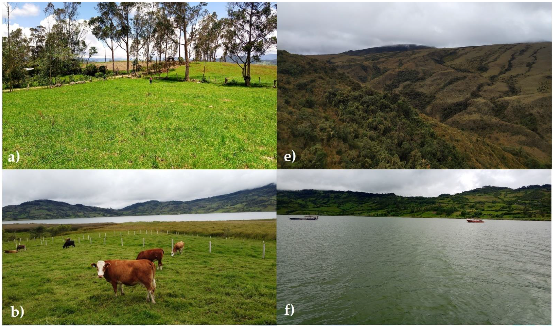
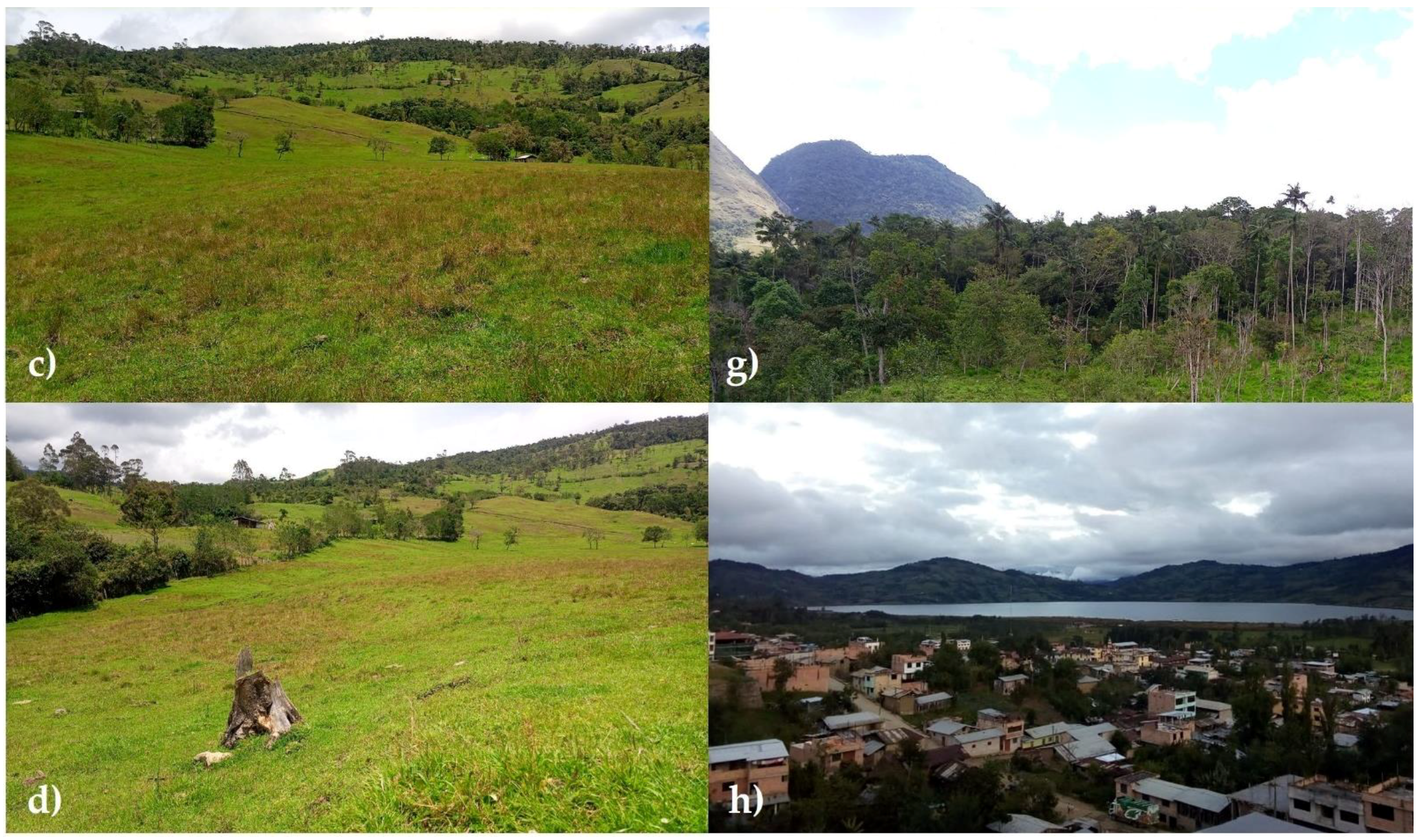
2.1. Study Area
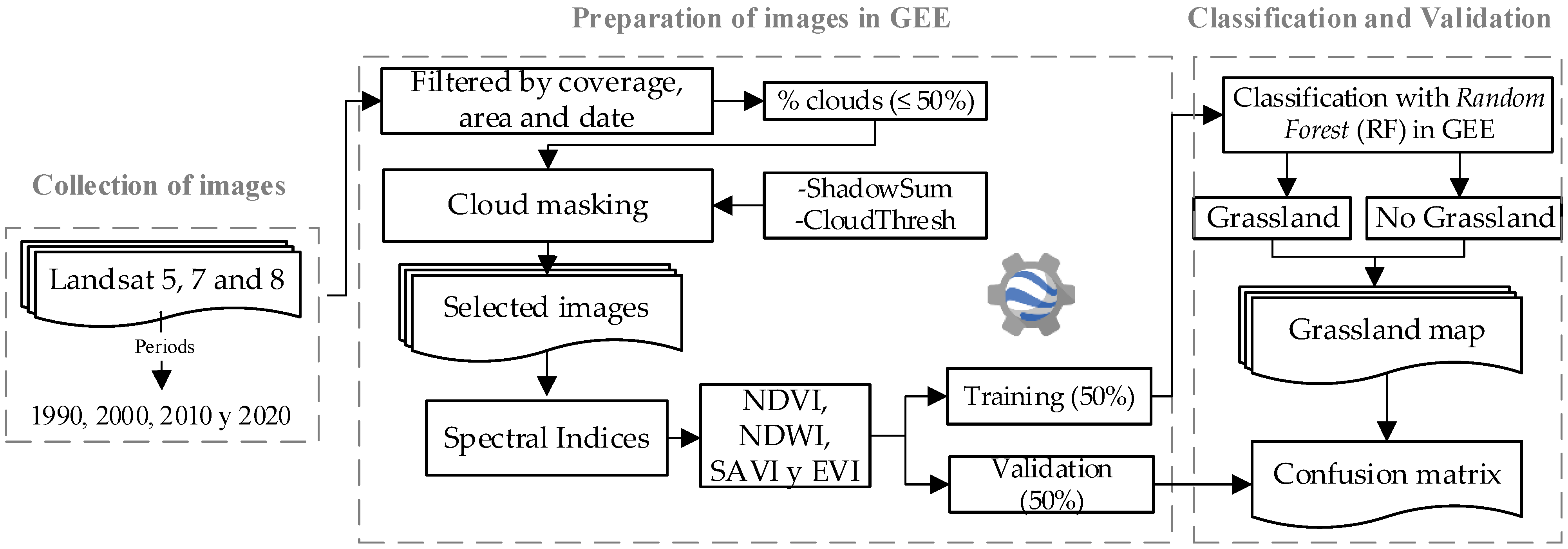
2.2. Methodological Design
2.3. Spatial Input Data
2.4. Preprocessing
2.5. Classification of Satellite Images
2.6. Intensity of Changes and Transition Matrices
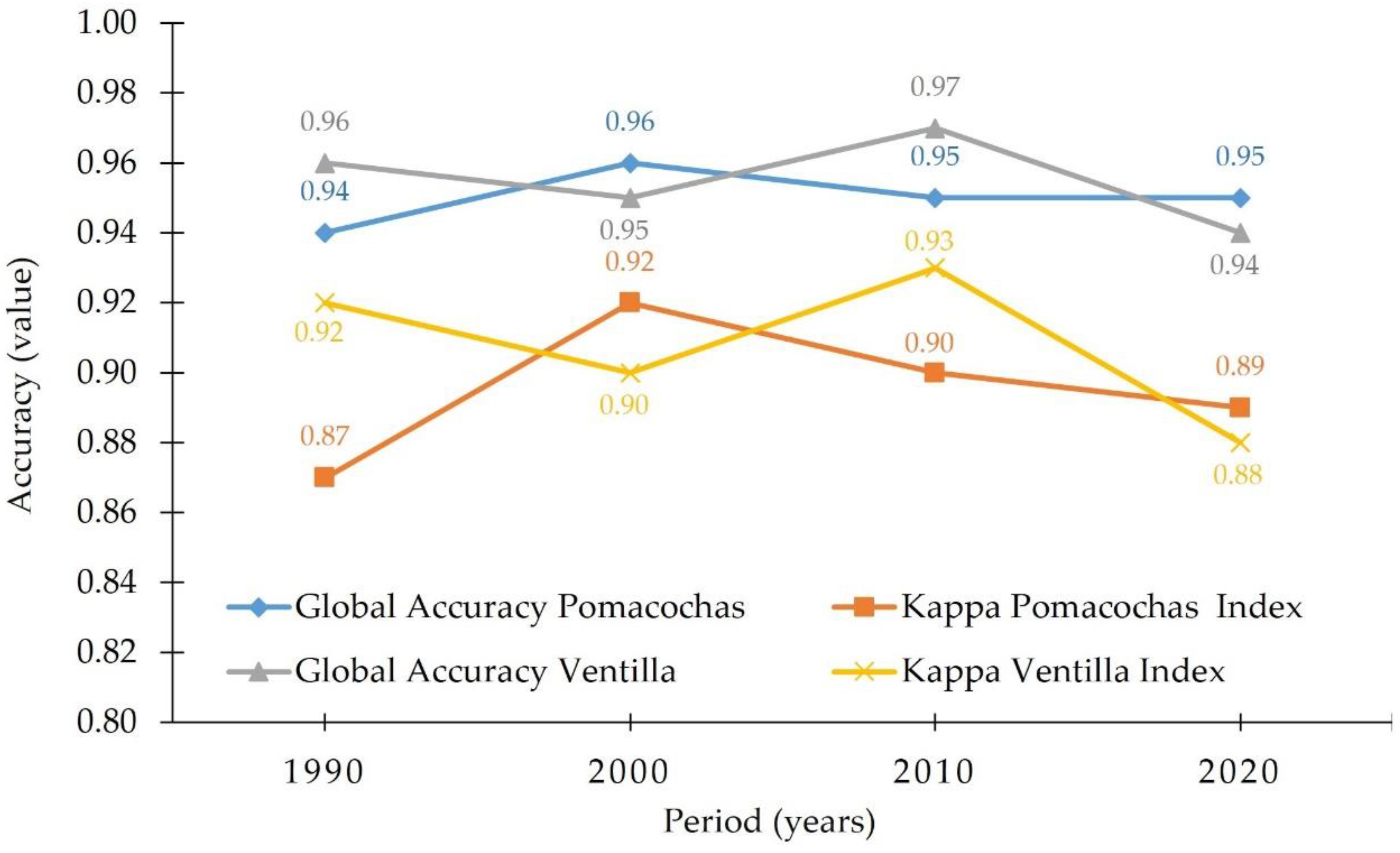
3. Results
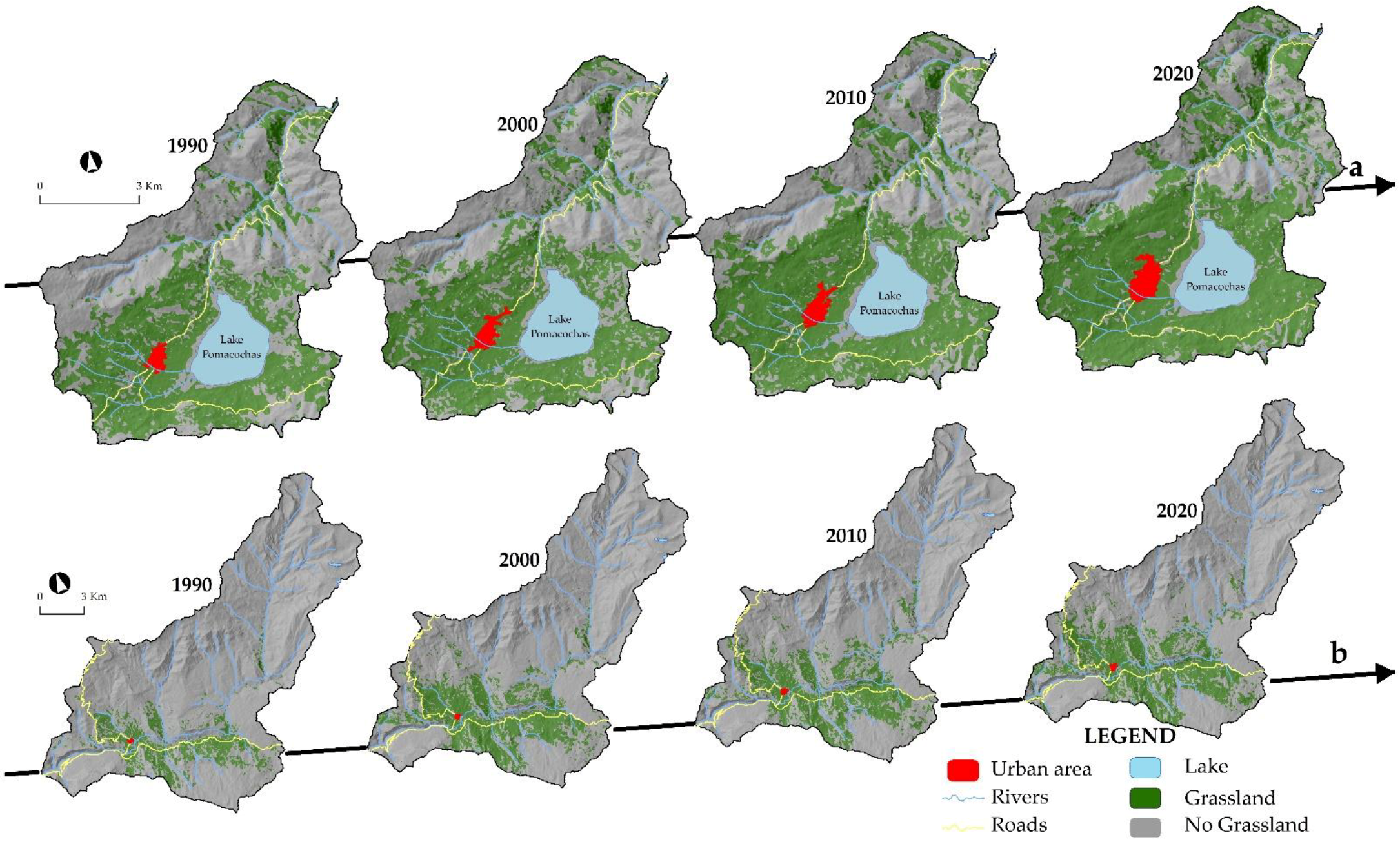
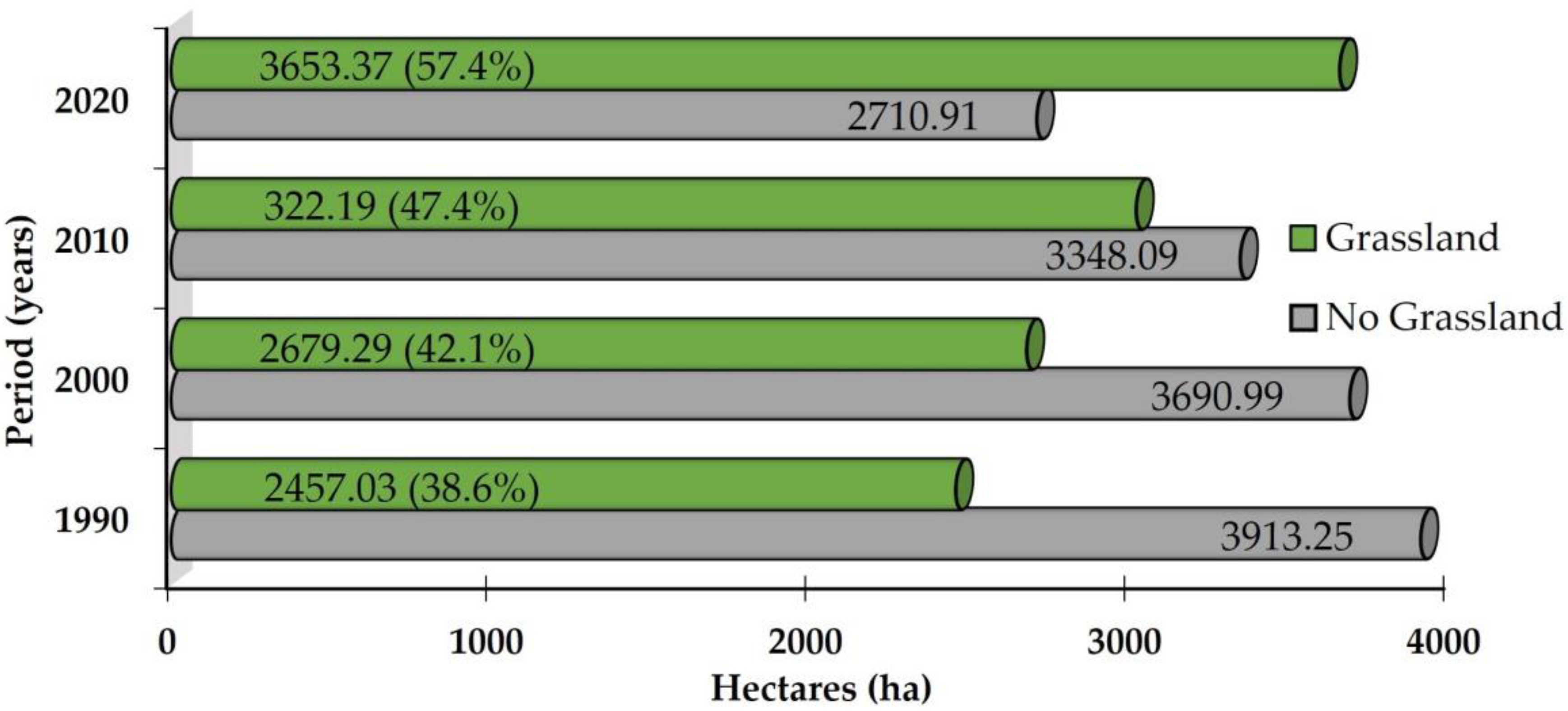
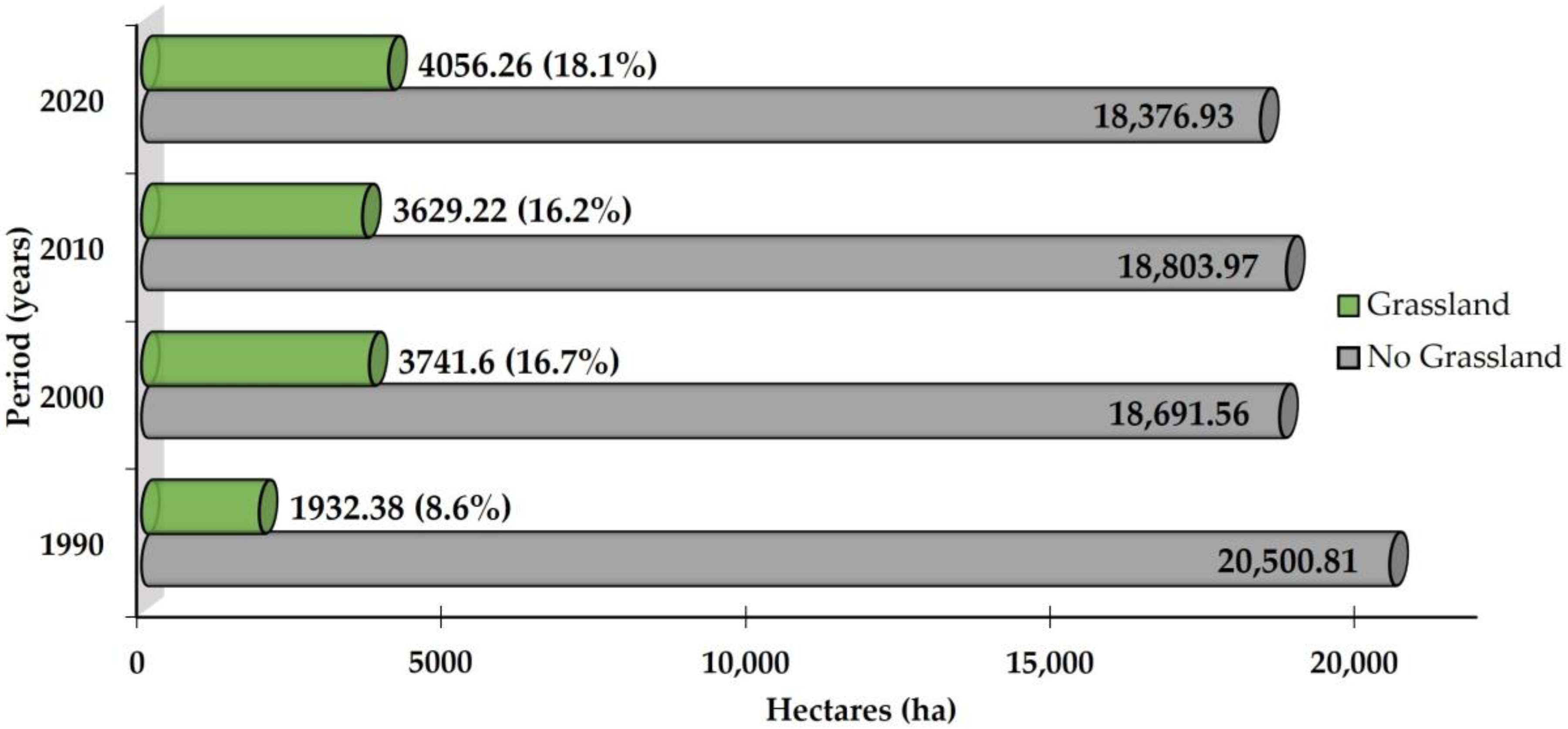
3.1. Grassland and Non-Grassland Maps
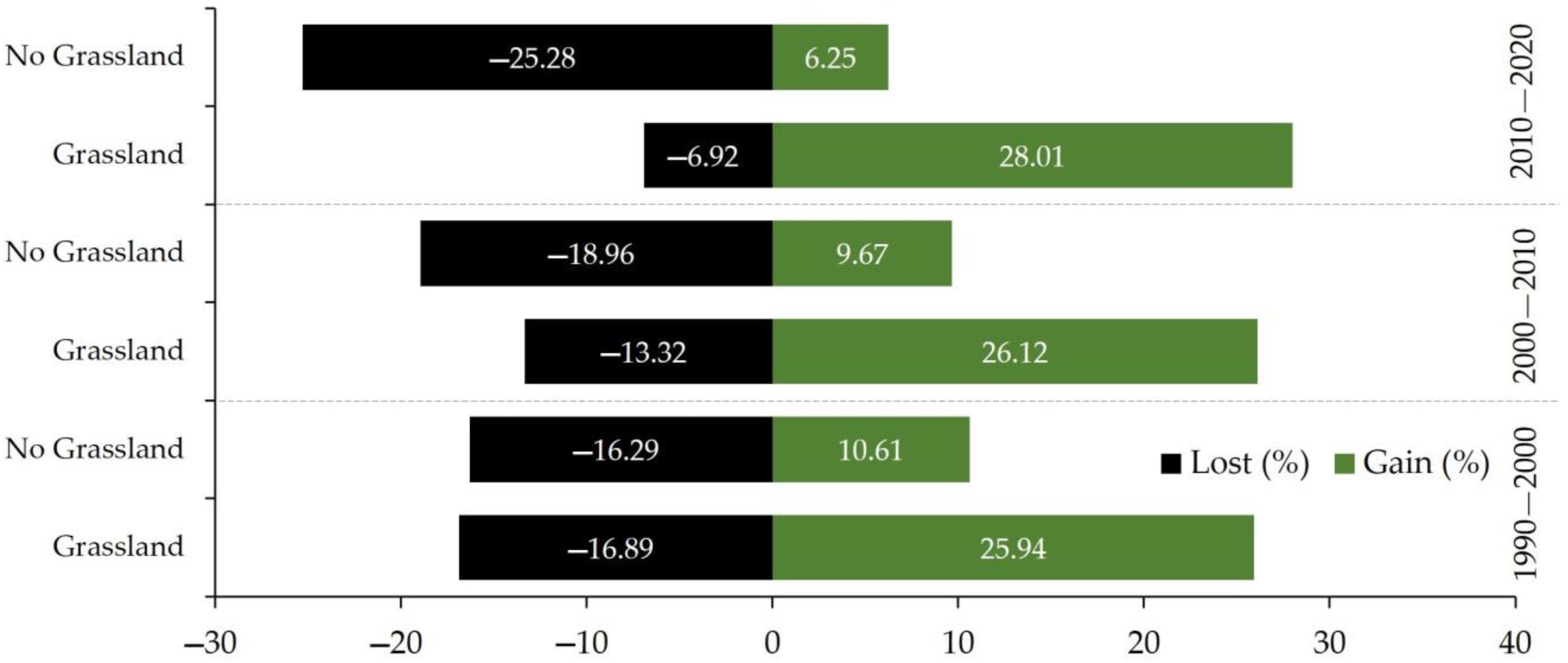
3.2. Exchange Rates (s)
3.3. Evaluation of Changes from Grassland to Non-Grassland by Period
4. Discussion
5. Conclusions
Supplementary Materials
Author Contributions
Funding
Institutional Review Board Statement
Informed Consent Statement
Data Availability Statement
Acknowledgments
Conflicts of Interest
References
- Wang, J.; Xiao, X.; Bajgain, R.; Starks, P.; Steiner, J.; Doughty, R.B.; Chang, Q. Estimating leaf area index and aboveground biomass of grazing pastures using sentinel-1, sentinel-2 and landsat images. ISPRS J. Photogramm. Remote Sens. 2019, 154, 189–201. [Google Scholar] [CrossRef] [Green Version]
- Umuhoza, J.; Jiapaer, G.; Yin, H.; Mind’je, R.; Gasirabo, A.; Nzabarinda, V.; Umwali, E.D. The analysis of grassland carrying capacity and its impact factors in typical mountain areas in central asia—A case of Kyrgyzstan and Tajikistan. Ecol. Indic. 2021, 131, 108129. [Google Scholar] [CrossRef]
- Blair, J.; Nippert, J.; Briggs, J. Grassland Ecology; Springer: Berlin/Heidelberg, Germany, 2014; ISBN 9781461475019. [Google Scholar]
- Flores, M. Captura de Dióxido de Carbono (CO2) en la “Chillihua” (Festuca Dolichophylla Presl) de los Pastizales del CIP-Illpa-Puno; Universidad Nacional del Altiplano Facultad de Ciencias Agrarias: Puno, Peru, 2017. [Google Scholar]
- Rebollo, S.; Gómez, A. Aprovechamiento Sostenible de los Pastizales. Ecosistemas 2003, 12, 7. Available online: https://www.revistaecosistemas.net/index.php/ecosistemas/article/view/231 (accessed on 6 November 2021).
- Lyu, X.; Li, X.; Dang, D.; Dou, H.; Xuan, X.; Liu, S. A new method for grassland degradation monitoring by vegetation species composition using hyperspectral remote sensing. Ecol. Indic. 2020, 114, 106310. [Google Scholar] [CrossRef]
- CONYCET. La Importancia de la Conservación de Pastizales. Available online: https://www.conicet.gov.ar/la-importancia-de-la-conservacion-de-pastizales/ (accessed on 21 December 2021).
- Cuesta, F.; Muriel, P.; Beck, S.; Meneses, R.I.; Halloy, S.; Salgado, S.; Ortiz, E.; Becerra, M.T. Biodiversidad y cambio climático en los andes tropicales. Rev. Virtual REDESMA 2012, 6, 180. [Google Scholar]
- Pérez, R. El lado oscuro de la ganadería. Probl. Desarro. 2008, 39, 217–227. [Google Scholar]
- Padilla, C.; Crespo, G.; Sardiñas, Y. Degradación y recuperación de pastizales. Rev. Cuba. Cienc. Agríc. 2009, 43, 351–354. [Google Scholar]
- Wang, M.P.; Zhao, C.Z.; Long, R.J.; Yang, Y.H. Rangeland governance in China: Overview, impacts on Sunan County in Gansu Province and future options. Rangel. J. 2010, 32, 155–163. [Google Scholar] [CrossRef]
- Mamani, S.J.; Servan, L.N. Evaluación Multitemporal de la Deforestación en El Distrito de Molinopampa, Provincia de Chachapoyas Departamento Amazonas 2015; Universidad Nacional Toribio Rodriguez de Mendoza de Amazonas: Chachapoyas, Peru, 2018. [Google Scholar]
- Chen, L.; Ma, Z.; Zhao, T. Modeling and analysis of the potential impacts on regional climate due to vegetation degradation over arid and semi-arid regions of China. Clim. Change 2017, 144, 461–473. [Google Scholar] [CrossRef]
- IPBES. Plataforma Intergubernamental Científico Normativa sobre Diversidad Biológica y Servicios de los Ecosistemas: Informe y Resumen para Tomadores de Decisiones de las Evaluaciones Regionales: África, América, Asia Pacífico, Europa y Asia Central; IPBES: Bonn, Germany, 2018. [Google Scholar]
- Bolt, C. Nuevo Atlas de Pastizales Revela la Importancia de los Pastizales Saludables Para la Vida Silvestre y Los Seres Humanos|Historias|Descubre WWF. Available online: https://www.worldwildlife.org/descubre-wwf/historias/nuevo-atlas-de-pastizales-revela-la-importancia-de-los-pastizales-saludables-para-la-vida-silvestre-y-los-seres-humanos (accessed on 17 September 2021).
- Zeme, S.; Entraigas, I.; Varni, M. Análisis de los servicios ecosistémicos en un pastizal natural de la pampa deprimida bonaerense. Contrib. Científicas GÆA 2015, 27, 161–174. [Google Scholar]
- Hott, M.C.; Carvalho, L.M.T.; Antunes, M.A.H.; Resende, J.C.; Rocha, W.S.D. Analysis of grassland degradation in Zona da Mata, MG, Brazil, based on NDVI time series data with the integration of phenological metrics. Remote Sens. 2019, 11, 2956. [Google Scholar] [CrossRef] [Green Version]
- Lu, H.; Raupach, M.R.; McVicar, T.R.; Barrett, D.J. Decomposition of vegetation cover into woody and herbaceous components using AVHRR NDVI time series. Remote Sens. Environ. 2003, 86, 1–18. [Google Scholar] [CrossRef]
- Fauvel, M.; Lopes, M.; Dubo, T.; Rivers-Moore, J.; Frison, P.L.; Gross, N.; Ouin, A. Prediction of plant diversity in grasslands using Sentinel-1 and -2 satellite image time series. Remote Sens. Environ. 2020, 237, 111536. [Google Scholar] [CrossRef]
- Ali, I.; Cawkwell, F.; Dwyer, E.; Barrett, B.; Green, S. Satellite remote sensing of grasslands: From observation to management. J. Plant Ecol. 2016, 9, 649–671. [Google Scholar] [CrossRef] [Green Version]
- Wachendorf, M.; Fricke, T.; Möckel, T. Remote sensing as a tool to assess botanical composition, structure, quantity and quality of temperate grasslands. Grass Forage Sci. 2018, 73, 1–14. [Google Scholar] [CrossRef]
- Gorelick, N.; Hancher, M.; Dixon, M.; Ilyushchenko, S.; Thau, D.; Moore, R. Google earth engine: Planetary-scale geospatial analysis for everyone. Remote Sens. Environ. 2017, 202, 18–27. [Google Scholar] [CrossRef]
- Tamiminia, H.; Salehi, B.; Mahdianpari, M.; Quackenbush, L.; Adeli, S.; Brisco, B. Google Earth Engine for geo-big data applications: A meta-analysis and systematic review. ISPRS J. Photogramm. Remote Sens. 2020, 164, 152–170. [Google Scholar] [CrossRef]
- Yu, R.; Yao, Y.; Wang, Q.; Wan, H.; Xie, Z.; Tang, W.; Zhang, Z.; Yang, J.; Shang, K.; Guo, X.; et al. Satellite-derived estimation of grassland aboveground biomass in the three-river headwaters region of China during 1982–2018. Remote Sens. 2021, 13, 2993. [Google Scholar] [CrossRef]
- Parente, L.; Ferreira, L. Assessing the spatial and occupation dynamics of the Brazilian Pasturelands based on the automated classification of MODIS images from 2000 to 2016. Remote Sens. Environ. 2018, 10, 606. [Google Scholar] [CrossRef] [Green Version]
- Peng, D.; Zhang, X.; Zhang, B.; Liu, L.; Liu, X.; Huete, A.R.; Huang, W.; Wang, S.; Luo, S.; Zhang, X.; et al. Scaling effects on spring phenology detections from MODIS data at multiple spatial resolutions over the contiguous United States. ISPRS J. Photogramm. Remote Sens. 2017, 132, 185–198. [Google Scholar] [CrossRef]
- Barboza, E.; Turpo Cayo, E.Y.; De Almeida, C.M.; Salas, R.; Rojas Briceño, N.B.; Silva López, J.O.; Barrena, M.Á.; Oliva, M.; Espinoza-Villar, R. Monitoring wildfires in the northeastern peruvian amazon using landsat-8 and sentinel-2 imagery in the GEE platform. ISPRS Int. J. Geo-Inf. 2020, 9, 564. [Google Scholar] [CrossRef]
- Amies, A.C.; Dymond, J.R.; Shepherd, J.D.; Pairman, D.; Hoogendoorn, C.; Sabetizade, M.; Belliss, S.E. National mapping of new zealand pasture productivity using temporal sentinel-2 data. Remote Sens. 2021, 13, 1481. [Google Scholar] [CrossRef]
- Serrano, J.; Shahidian, S.; Paixão, L.; Marques da Silva, J.; Morais, T.; Teixeira, R.; Domingos, T. Spatiotemporal patterns of pasture quality based on ndvi time-series in mediterranean montado ecosystem. Remote Sens. 2021, 13, 3820. [Google Scholar] [CrossRef]
- Tangud, T.; Nasahara, K.; Borjigin, H.; Bagan, H. Land-cover change in the Wulagai grassland, Inner Mongolia of China between 1986 and 2014 analysed using multi-temporal Landsat images. Geocarto Int. 2019, 34, 1237–1251. [Google Scholar] [CrossRef]
- Parente, L.; Mesquita, V.; Miziara, F.; Baumann, L.; Ferreira, L. Assessing the pasturelands and livestock dynamics in brazil, from 1985 to 2017: A novel approach based on high spatial resolution imagery and google earth engine cloud computing. Remote Sens. Environ. 2019, 232, 111301. [Google Scholar] [CrossRef]
- Fassnacht, F.E.; Li, L.; Fritz, A. Mapping degraded grassland on the Eastern Tibetan Plateau with multi-temporal Landsat 8 data —Where do the severely degraded areas occur? Int. J. Appl. Earth Obs. Geoinf. 2015, 42, 115–127. [Google Scholar] [CrossRef]
- Fernández-Habas, J.; García Moreno, A.M.; Hidalgo-Fernández, M.T.; Leal-Murillo, J.R.; Abellanas Oar, B.; Gómez-Giráldez, P.J.; González-Dugo, M.P.; Fernández-Rebollo, P. Investigating the potential of Sentinel-2 configuration to predict the quality of Mediterranean permanent grasslands in open woodlands. Sci. Total Environ. 2021, 791, 148101. [Google Scholar] [CrossRef]
- Matsushita, B.; Yang, W.; Chen, J.; Onda, Y.; Qiu, G. Sensitivity of the enhanced vegetation index (EVI) and normalized difference vegetation index (NDVI) to topographic effects: A case study in high-density cypress forest. Sensors 2007, 7, 2636–2651. [Google Scholar] [CrossRef] [Green Version]
- Elbeltagi, A.; Aslam, M.R.; Malik, A.; Mehdinejadiani, B.; Srivastava, A.; Bhatia, A.S.; Deng, J. The impact of climate changes on the water footprint of wheat and maize production in the Nile Delta, Egypt. Sci. Total Environ. 2020, 743, 140770. [Google Scholar] [CrossRef]
- La Cecilia, D.; Toffolon, M.; Woodcock, C.E.; Fagherazzi, S. Interactions between river stage and wetland vegetation detected with a seasonality index derived from LANDSAT images in the Apalachicola delta, Florida. Adv. Water Resour. 2016, 89, 10–23. [Google Scholar] [CrossRef] [Green Version]
- Cord, A.F.; Brauman, K.A.; Chaplin-Kramer, R.; Huth, A.; Ziv, G.; Seppelt, R. Priorities to advance monitoring of ecosystem services using earth observation. Trends Ecol. Evol. 2017, 32, 416–428. [Google Scholar] [CrossRef] [PubMed]
- Huete, A.R.; Didan, K.; Van Leeuwen, W. Modis vegetation index. Veg. Index Phenol. Lab 1999, 3, 129. [Google Scholar]
- Rouse, J.W.; Hass, R.H.; Schell, J.A.; Deering, D.W. Monitoring Vegetation Systems in the Great Plains with ERTS. In Proceedings of the Third Earth Resources Technology Satellite-1 Symposium, Washington, DC, USA, 10–14 December 1973; Volume 1, pp. 309–317. [Google Scholar]
- Gao, X.; Huete, A.R.; Ni, W.; Miura, T. Optical-biophysical relationships of vegetation spectra without background contamination. Remote Sens. Environ. 2000, 74, 609–620. [Google Scholar] [CrossRef]
- Gao, X.; Huete, A.R.; Didan, K. Multisensor comparisons and validation of MODIS vegetation indices at the semiarid jornada experimental range. IEEE Trans. Geosci. Remote Sens. 2003, 41, 2368–2381. [Google Scholar] [CrossRef]
- Huete, A.R. A soil-adjusted vegetation index (SAVI). Remote Sens. Environ. 1988, 25, 295–309. [Google Scholar] [CrossRef]
- Kumari, N.; Srivastava, A.; Dumka, U.C. A long-term spatiotemporal analysis of vegetation greenness over the himalayan region using google earth engine. Climate 2021, 9, 109. [Google Scholar] [CrossRef]
- Edirisinghe, A.; Clark, D.; Waugh, D. Spatio-temporal modelling of biomass of intensively grazed perennial dairy pastures using multispectral remote sensing. Int. J. Appl. Earth Obs. Geoinf. 2012, 16, 5–16. [Google Scholar] [CrossRef]
- Shelestov, A.; Lavreniuk, M.; Kussul, N.; Novikov, A.; Skakun, S. Exploring google earth engine platform for big data processing: Classification of multi-temporal satellite imagery for crop mapping. Front. Earth Sci. 2017, 5, 17. [Google Scholar] [CrossRef] [Green Version]
- Wang, J.; Xiao, X.; Qin, Y.; Dong, J.; Geissler, G.; Zhang, G.; Cejda, N.; Alikhani, B.; Doughty, R.B. Mapping the dynamics of eastern redcedar encroachment into grasslands during 1984–2010 through PALSAR and time series landsat images. Remote Sens. Environ. 2017, 190, 233–246. [Google Scholar] [CrossRef] [Green Version]
- Oliva, M.; Collazos, R.; Vásquez, H.; Rubio, K.; Maicelo, J.L. Floristic composition of herbaceous forage species in natural prairies of the main livestock watersheds of the Amazon region. Sci. Agropecu. 2019, 10, 109–117. [Google Scholar] [CrossRef]
- Manuel, O.; Diórman, R.; Antonio, M.; Carmen, O.; Mario, A.O. Nutritional content, digestibility and performance of native grasses biomass that dominate livestock Molinopampa, Pomacochas and Leymebamba basins, Amazonas, Peru. Sci. Agropecu. 2015, 6, 211–215. [Google Scholar] [CrossRef] [Green Version]
- Caro, C.; Sánchez, E.; Quinteros, Z.; Castañeda, L. Respuesta de los pastizales altoandinos a la perturbación generada por extracción mediante la actividad de “Champeo” en los terrenos de la comunidad campesina Villa De Junín, Perú. Ecol. Apl. 2014, 13, 85. [Google Scholar] [CrossRef] [Green Version]
- Tovar, O. Estudio florístico de los pastizales de la costa Norte Del Perú. Rev. Peru. Biol. 2005, 12, 397–416. [Google Scholar] [CrossRef]
- MINAGRI. Plan Nacional de Desarrollo Ganadro 2017–2027; Lima, Perú. 2017. Available online: https://www.midagri.gob.pe/portal/download/pdf/dg-ganaderia/plan-nacional-ganadero-2017-2027.pdf (accessed on 25 November 2021).
- Estrada Zuñiga, A.C.; Zapana Pari, J.G. Capacidad de carga de pastos de puna húmeda en un contexto de cambio climático. Rev. Investig. Altoandinas J. High Andean Res. 2018, 20, 361–379. [Google Scholar] [CrossRef]
- Pasricha, N.S.; Ghosh, P.K. Soil organic carbon dynamics in tropical and subtropical grassland ecosystem. In Carbon Management in Tropical and Sub-Tropical Terrestrial Systems; Springer: Singapore, 2019; pp. 283–297. [Google Scholar] [CrossRef]
- Rolando, J.L.; Dubeux, J.C.B.; Ramirez, D.A.; Ruiz-Moreno, M.; Turin, C.; Mares, V.; Sollenberger, L.E.; Quiroz, R. Land use effects on soil fertility and nutrient cycling in the peruvian high-andean puna grasslands. Soil Sci. Soc. Am. J. 2018, 82, 463–474. [Google Scholar] [CrossRef]
- Rodríguez, A.F.; Limachi, H.L.; Reátegui, R.F.; Escobedo, T.R.; Ramírez, B.J.; Encarnación, C.F.; Maco, G.J.; Guzman, C.W.; Castro, M.W.; Fachin, M.L.; et al. Zonificación Ecológica y Económica (ZEE) del Departamento de Amazonas; Instituto de Investigaciones de la Amazonía Peruana: Iquitos, Peru, 2010; Available online: https://alicia.concytec.gob.pe/vufind/Record/IIAP_9c9763ff6479f6a1b3956d99a0fb6b7e (accessed on 2 February 2022).
- Briceño, N.B.R.; Castillo, E.B.; Torres, O.A.G.; Oliva, M.; Tafur, D.L.; Gurbillón, M.Á.B.; Corroto, F.; López, R.S.; Rascón, J. Morphometric prioritization, fluvial classification, and hydrogeomorphological quality in high Andean livestock micro-watersheds in northern Peru. ISPRS Int. J. Geo-Inf. 2020, 9, 305. [Google Scholar] [CrossRef]
- Ruiz, R.E.; Saucedo-Uriarte, J.A.; Portocarrero-Villegas, S.M.; Quispe-Ccasa, H.A.; Cayo-Colca, I.S. Zoometric characterization of creole cows from the Southern Amazon region of Peru. Diversity 2021, 13, 510. [Google Scholar] [CrossRef]
- Ramírez, J.M. Uso Actual de la Tierra, Informe Temático. Proyecto Zonificación Ecológica y Económica del Departamento de Amazonas; Iquitos, Peru, 2010. Available online: http://terra.iiap.gob.pe/assets/files/macro/zee-amazonas/02_Geologia_2010.pdf (accessed on 15 February 2022).
- Murga, L.; Vásquez, H.; Bardales, J. Caracterización de los sistemas de producción de ganado bovino en las cuencas ganaderas de Ventilla, Florida y Leyva -región Amazonas. Rev. Científica UNTRM Cienc. Nat. Ing. 2019, 1, 28–37. [Google Scholar] [CrossRef]
- Vásquez, H.V.; Valqui, L.; Castillo, M.S.; Alegre, J.; Gómez, C.A.; Bobadilla, L.G.; Maicelo, J.L. Caracterización de sistemas silvopastoriles en la cuenca ganadera de molinopampa, zona noroccidental del Perú. Temas Agrar. 2020, 25, 23–34. [Google Scholar] [CrossRef]
- Masek, J.G.; Vermote, E.F.; Saleous, N.E.; Wolfe, R.; Hall, F.G.; Huemmrich, K.F.; Gao, F.; Kutler, J.; Teng-Kui, L. A landsat surface reflectance dataset for North America, 1990–2000. IEEE Geosci. Remote Sens. Lett. 2006, 3, 68–72. [Google Scholar] [CrossRef]
- Chuvieco, E. Fundamentals of Satellite Remote Sensing. An Environmental Approach, 2nd ed.; CRC Press: Boca Raton, FL, USA, 2016; ISBN 9781498728072. [Google Scholar]
- Souza, C.M.; Shimbo, J.Z.; Rosa, M.R.; Parente, L.L.; Alencar, A.A.; Rudorff, B.F.T.; Hasenack, H.; Matsumoto, M.; Ferreira, L.G.; Souza-Filho, P.W.M.; et al. Reconstructing three decades of land use and land cover changes in brazilian biomes with landsat archive and earth engine. Remote Sens. 2020, 12, 2735. [Google Scholar] [CrossRef]
- Foga, S.; Scaramuzza, P.L.; Guo, S.; Zhu, Z.; Dilley, R.D.; Beckmann, T.; Schmidt, G.L.; Dwyer, J.L.; Joseph Hughes, M.; Laue, B. Cloud detection algorithm comparison and validation for operational Landsat data products. Remote Sens. Environ. 2017, 194, 379–390. [Google Scholar] [CrossRef] [Green Version]
- Housman, I.W.; Chastain, R.A.; Finco, M.V. An evaluation of forest health insect and disease survey data and satellite-based remote sensing forest change detection methods: Case studies in the United States. Remote Sens. 2018, 10, 1184. [Google Scholar] [CrossRef] [Green Version]
- McFeeters, S.K. The use of the normalized difference water index (NDWI) in the delineation of open water features. Int. J. Remote Sens. 1996, 17, 1425–1432. [Google Scholar] [CrossRef]
- Zhu, Z.; Bi, J.; Pan, Y.; Ganguly, S.; Anav, A.; Xu, L.; Samanta, A.; Piao, S.; Nemani, R.R.; Myneni, R.B. Global data sets of vegetation leaf area index (LAI)3g and fraction of photosynthetically active radiation (FPAR)3g derived from global inventory modeling and mapping studies (GIMMS) normalized difference vegetation index (NDVI3G) for the period 1981 to 2. Remote Sens. 2013, 5, 927–948. [Google Scholar] [CrossRef] [Green Version]
- Tucker, C.J. Red and photographic infrared linear combinations for monitoring vegetation. Remote Sens. Environ. 1979, 8, 127–150. [Google Scholar] [CrossRef] [Green Version]
- Huete, A.; Didan, K.; Miura, T.; Rodriguez, E..; Gao, X.; Ferreira, L. Overview of the radiometric and biophysical performance of the MODIS vegetation indices. Remote Sens. 2002, 83, 1967. [Google Scholar] [CrossRef]
- Ren, H.; Zhou, G.; Zhang, F. Using negative soil adjustment factor in soil-adjusted vegetation index (SAVI) for aboveground living biomass estimation in arid grasslands. Remote Sens. Environ. 2018, 209, 439–445. [Google Scholar] [CrossRef]
- Rhyma, P.P.; Norizah, K.; Hamdan, O.; Faridah-Hanum, I.; Zulfa, A.W. Integration of normalised different vegetation index and Soil-Adjusted Vegetation Index for mangrove vegetation delineation. Remote Sens. Appl. Soc. Environ. 2020, 17, 100280. [Google Scholar] [CrossRef]
- Breiman, L.E.O. Random forests. Mach. Learn. 2001, 45, 5–32. [Google Scholar] [CrossRef] [Green Version]
- Tsai, Y.H.; Stow, D.; Chen, H.L.; Lewison, R.; An, L.; Shi, L. Mapping vegetation and land use types in Fanjingshan National Nature Reserve using google earth engine. Remote Sens. 2018, 10, 927. [Google Scholar] [CrossRef] [Green Version]
- FAO. Global Forest Resources Assessment 2000 Main Report; FAO: Rome, Italy, 2001. [Google Scholar]
- MINAM. Protocolo: Evaluacion de la Exactitud Tematica del Mapa de Deforestación; MINAM: Lima, Perú, 2014. [Google Scholar]
- Padilla, M.; Stehman, S.V.; Chuvieco, E. Validation of the 2008 MODIS-MCD45 global burned area product using strati fi ed random sampling. Remote Sens. Environ. 2014, 144, 187–196. [Google Scholar] [CrossRef]
- Rojas, N.B.; Castillo, E.B.; Quintana, J.L.M.; Cruz, S.M.O.; López, R.S. Deforestation in the peruvian Amazon: Indexes of land cover/land use (LC/LU) changes based on GIS. Boletín De La Asociación De Geógrafos Españoles. 2019, 81, 1–34. [Google Scholar] [CrossRef]
- Pontius, R.G.; Shusas, E.; McEachern, M. Detecting important categorical land changes while accounting for persistence. Agric. Ecosyst. Environ. 2004, 101, 251–268. [Google Scholar] [CrossRef]
- Pettorelli, N.; Vik, J.O.; Mysterud, A.; Gaillard, J.M.; Tucker, C.J.; Stenseth, N.C. Using the satellite-derived NDVI to assess ecological responses to environmental change. Trends Ecol. Evol. 2005, 20, 503–510. [Google Scholar] [CrossRef] [PubMed]
- Chávez, R.O.; Clevers, J.G.P.W.; Decuyper, M.; de Bruin, S.; Herold, M. 50 years of water extraction in the Pampa del Tamarugal basin: Can prosopis tamarugo trees survive in the hyper-arid Atacama Desert (Northern Chile)? J. Arid Environ. 2016, 124, 292–303. [Google Scholar] [CrossRef]
- Gitelson, A.A. Wide dynamic range vegetation index for remote quantification of biophysical characteristics of vegetation. J. Plant Physiol. 2004, 161, 165–173. [Google Scholar] [CrossRef] [PubMed] [Green Version]
- Guzman, J.; Atkinson, P.M.; Dash, J.; Rioja-Nieto, R. Spatiotemporal variation in mangrove chlorophyll concentration using Landsat 8. Remote Sens. 2015, 7, 14530–14558. [Google Scholar] [CrossRef] [Green Version]
- Huang, S.; Tang, L.; Hupy, J.P.; Wang, Y.; Shao, G. A commentary review on the use of normalized difference vegetation index (NDVI) in the era of popular remote sensing. J. For. Res. 2020, 32, 2719. [Google Scholar] [CrossRef]
- NASA. MODIS Land Cover Type/Dynamics. Available online: https://modis.gsfc.nasa.gov/data/dataprod/mod12.php (accessed on 18 November 2021).
- EUMETSAT. AVHRR Advanced Very High Resolution Radiometer. Available online: https://www.eumetsat.int/avhrr (accessed on 25 December 2021).
- Wu, G.; De Leeuw, J.; Skidmore, A.; Prins, H.; Liu, Y. Comparison of MODIS and Landsat TM5 images for mapping tempo-spatial dynamics of Secchi disk depths in Poyang Lake National Nature Reserve, China. Int. J. Remote Sens. 2008, 29, 2183–2198. [Google Scholar] [CrossRef]
- Salas, R.; Barboza, E.; Oliva, S.M. Dinámica multitemporal de índices de deforestación en el distrito de Florida, departamento de Amazonas, Perú. INDES Rev. Investig. Desarro. Sustent. 2016, 2, 18–27. [Google Scholar] [CrossRef]
- Oliva, M.; Maicelo Quintana, J.L.; Torres Guzmán, C.; Bardales Escalante, W. Propiedades fisicoquímicas del suelo en diferentes estadios de la agricultura migratoria en el Área de Conservación Privada “Palmeras de Ocol”, distrito de Molinopampa, provincia de Chachapoyas (departamento de Amazonas). Rev. Investig. Agroproducc. Sustent. 2017, 1, 9–21. [Google Scholar] [CrossRef]
- Oliva, M.; Oliva, C.; Rojas, D.; Oliva, M.; Morales, A. Botanical identification of native species most important of dairy basins molinopampa, pomacochas and leymebamba, amazonas, Peru. Sci. Agropecu. 2015, 6, 125–129. [Google Scholar] [CrossRef] [Green Version]
- Smith, P.; Gregory, P.J.; Van Vuuren, D.; Obersteiner, M.; Havlík, P.; Rounsevell, M.; Woods, J.; Stehfest, E.; Bellarby, J. Competition for land. Philos. Trans. R. Soc. B Biol. Sci. 2010, 365, 2941–2957. [Google Scholar] [CrossRef] [Green Version]
- Alkimim, A.; Sparovek, G.; Clarke, K.C. Converting Brazil’s pastures to cropland: An alternative way to meet sugarcane demand and to spare forestlands. Appl. Geogr. 2015, 62, 75–84. [Google Scholar] [CrossRef]
- Thorvaldsson, G.; Bjornsson, H.; Hermannsson, J. The influence of weather on early growth rate of grasses. Búvísindi 2005, 9, 65–73. [Google Scholar]
- Han, G.; Hao, X.; Zhao, M.; Wang, M.; Ellert, B.H.; Willms, W.; Wang, M. Effect of grazing intensity on carbon and nitrogen in soil and vegetation in a meadow steppe in Inner Mongolia. Agric. Ecosyst. Environ. 2008, 125, 21–32. [Google Scholar] [CrossRef]
- Wang, Y.; Zhou, G.; Jia, B. Modeling SOC and NPP responses of meadow steppe to different grazing intensities in Northeast China. Ecol. Model. 2008, 217, 72–78. [Google Scholar] [CrossRef]
- Liu, Y.; Zhang, Z.; Tong, L.; Khalifa, M.; Wang, Q.; Gang, C.; Wang, Z.; Li, J.; Sun, Z. Assessing the effects of climate variation and human activities on grassland degradation and restoration across the globe. Ecol. Indic. 2019, 106, 105504. [Google Scholar] [CrossRef]
- Xu, B.; Yang, X.C.; Tao, W.G.; Qin, Z.H.; Liu, H.Q.; Miao, J.M.; Bi, Y.Y. Modis-based remote sensing monitoring of grass production in China. Int. J. Remote Sens. 2008, 29, 5313–5327. [Google Scholar] [CrossRef]
- Contreras, J.R.; Volke, V.; Oropeza, J.L.; Rodriguez, C.; Martínez, T.; Martínez, A. Estado actual y causas de la degradación de los agostaderos en el municipio deYanhuitlán, Oaxaca. Terra Latinoam. 2003, 21, 427–435. [Google Scholar]
- Tovar, C.; Seijmonsbergen, A.C.; Duivenvoorden, J.F. Monitoring land use and land cover change in mountain regions: An example in the Jalca grasslands of the Peruvian Andes. Landsc. Urban Plan. 2013, 112, 40–49. [Google Scholar] [CrossRef]
- Opazo, S.; Garay, E.; Muñoz, R.; López-Saldaña, G.; Aguilar, R.; Radic, S. Desarrollo de una plataforma web sig para el monitoreo dinámico de pastizales en magallania. An. Inst. Patagon. 2014, 42, 39–51. [Google Scholar] [CrossRef] [Green Version]
- Zhao, W.; Luo, T.; Wei, H.; Zhang, L. Relative impact of climate change and grazing on NDVI changes in grassland in the Mt. Qomolangma nature reserve and adjacent regions during 2000–2018. Diversity 2022, 14, 171. [Google Scholar] [CrossRef]
- Li, Q.; Wang, J.; Xie, H.; Ochir, A. Applicability of grassland production estimation using remote sensing for the Mongolian Plateau by comparing typical regions in China and Mongolia. Sustainability 2022, 14, 3122. [Google Scholar] [CrossRef]


| Collection | No. of Images * (Cloud Cover < 50%) | |||||||
|---|---|---|---|---|---|---|---|---|
| Ventilla Micro-Watershed ** | Pomacochas Micro-Watershed ** | |||||||
| 1900 | 2000 | 2010 | 2020 | 1900 | 2000 | 2010 | 2020 | |
| LANDSAT/LT05/C01/T1_SR | 7 | 3 | 4 | 2 | 2 | 2 | ||
| LANDSAT/LE07/C01/T1_SR | 2 | 3 | ||||||
| LANDSAT/LC08/C01/T1_SR | 12 | 3 | ||||||
| Name | Abbreviation | Formula | Source |
|---|---|---|---|
| Normalized Difference Vegetation Index | NDVI | [39] | |
| Enhanced Vegetation Index | EVI | [41] | |
| Soil-Adjusted Vegetation Index | SAVI | [42] | |
| Normalized Difference Water Index | NDWI | [66] |
| Class | 1990 | 2000 | 2010 | 2020 | 1990–2020 | |||||
| ha | % | ha | % | ha | % | ha | % | ha | % | |
| Pomacochas | ||||||||||
| Grassland | 2457.03 | 38.6 | 2679.29 | 42.1 | 3022.19 | 47.4 | 3659.37 | 57.4 | 1202.34 | 48.9 |
| No-grassland | 3913.25 | 61.4 | 3690.99 | 57.9 | 3348.09 | 52.6 | 2710.91 | 42.6 | −1202.34 | −30.7 |
| Total | 6370.28 | 100 | 6370.28 | 100 | 6370.28 | 100 | 6370.28 | 100 | ||
| Ventilla | ||||||||||
| Grassland | 1932.38 | 8.6 | 3741.63 | 16.7 | 3629.22 | 16.2 | 4056.26 | 18.1 | 2123.88 | 109.9 |
| No-grassland | 20,500.81 | 91.4 | 18,691.56 | 83.3 | 18,803.97 | 83.8 | 18,376.93 | 81.9 | −2123.88 | −10.4 |
| Total | 22,433.19 | 100 | 22,433.19 | 100 | 22,433.19 | 100 | 22,433.19 | 100 | ||
| Period | Year 1 | Year 2 | Total Year 2 (ha) | Exchange Rate (s) | Loss | Total Change | Net Change | Exchange | |
|---|---|---|---|---|---|---|---|---|---|
| (Year 1–Year 2) | Grassland | No-Grassland | Percentage (%) | ||||||
| 1990–2000 | Grassland | 2042.01 | 415.02 | 2457.03 | 0.87 | 16.89 | 42.83 | 9.05 | 33.78 |
| No-grassland | 637.28 | 3275.97 | 3913.25 | −0.58 | 16.29 | 26.89 | 5.68 | 21.21 | |
| Total Year 1 (ha) | 2679.29 | 3690.99 | 6370.28 | ||||||
| Gain (%) | 25.94 | 10.61 | |||||||
| 2000–2010 | Grassland | 2322.37 | 356.92 | 2679.29 | 1.21 | 13.32 | 39.44 | 12.80 | 26.64 |
| No-grassland | 699.82 | 2991.17 | 3690.99 | −0.97 | 18.96 | 28.63 | 9.29 | 19.34 | |
| Total Year 1 (ha) | 3022.19 | 3348.09 | 6370.28 | ||||||
| Gain (%) | 26.12 | 9.67 | |||||||
| 2010–2020 | Grassland | 2812.93 | 209.26 | 3022.19 | 1.93 | 6.92 | 34.93 | 21.08 | 13.85 |
| No-grassland | 846.45 | 2501.64 | 3348.09 | −2.09 | 25.28 | 31.53 | 19.03 | 12.50 | |
| Total Year 1 (ha) | 3659.38 | 2710.90 | 6370.28 | ||||||
| Gain (%) | 28.01 | 6.25 | |||||||
| Period | Year 1 | Year 2 | Total Year 2 (ha) | Exchange Rate (s) | Loss | Total Change | Net Change | Exchange | |
|---|---|---|---|---|---|---|---|---|---|
| (Year 1–Year 2) | Grassland | No-Grassland | Percentage (%) | ||||||
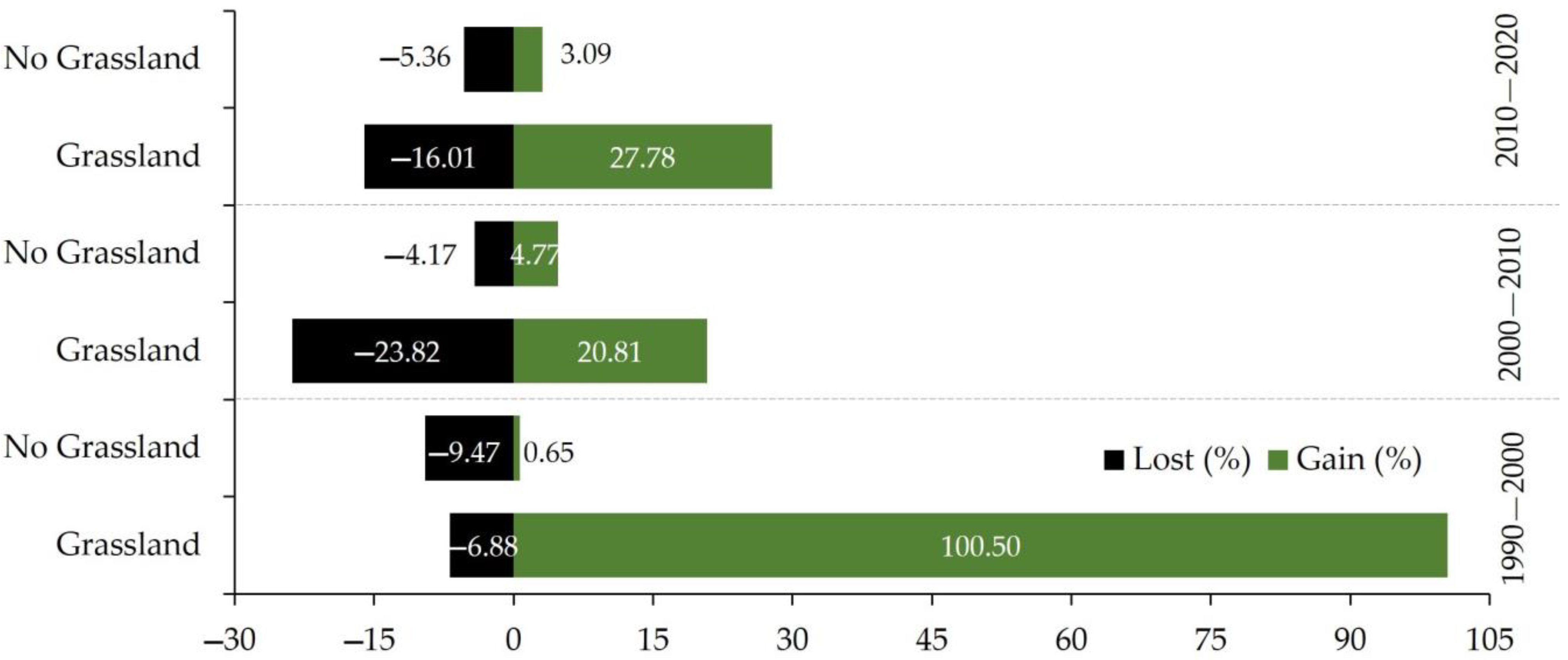
| 1990–2000 | Grassland | 1799.53 | 132.86 | 1932.39 | 6.83 | 6.88 | 107.38 | 93.63 | 13.75 |
| No-grassland | 1942.10 | 18,558.70 | 20,500.80 | −0.92 | 9.47 | 10.12 | 8.83 | 1.30 | |
| Total Year 1 (ha) | 3741.63 | 18,691.56 | 22,433.19 | ||||||
| Gain (%) | 100.50 | 0.65 | |||||||
| 2000–2010 | Grassland | 2850.42 | 891.21 | 3741.63 | −0.30 | 23.82 | 44.63 | 3.00 | 41.63 |
| No-grassland | 778.80 | 17,912.76 | 18,691.56 | 0.06 | 4.17 | 8.93 | 0.60 | 8.33 | |
| Total Year 1 (ha) | 3629.22 | 18,803.97 | 22,433.19 | ||||||
| Gain (%) | 20.81 | 4.77 | |||||||
| 2010–2020 | Pasture | 3048.12 | 581.11 | 3629.23 | 1.12 | 16.01 | 43.79 | 11.77 | 32.02 |
| No-grassland | 1008.14 | 17,795.82 | 18,803.96 | −0.23 | 5.36 | 8.45 | 2.27 | 6.18 | |
| Total Year 1 (ha) | 4056.26 | 18,376.93 | 22,433.19 | ||||||
| Gain (%) | 27.78 | 3.09 | |||||||
Publisher’s Note: MDPI stays neutral with regard to jurisdictional claims in published maps and institutional affiliations. |
© 2022 by the authors. Licensee MDPI, Basel, Switzerland. This article is an open access article distributed under the terms and conditions of the Creative Commons Attribution (CC BY) license (https://creativecommons.org/licenses/by/4.0/).
Share and Cite
Marin, N.A.; Barboza, E.; López, R.S.; Vásquez, H.V.; Gómez Fernández, D.; Terrones Murga, R.E.; Rojas Briceño, N.B.; Oliva-Cruz, M.; Gamarra Torres, O.A.; Silva López, J.O.; et al. Spatiotemporal Dynamics of Grasslands Using Landsat Data in Livestock Micro-Watersheds in Amazonas (NW Peru). Land 2022, 11, 674. https://doi.org/10.3390/land11050674
Marin NA, Barboza E, López RS, Vásquez HV, Gómez Fernández D, Terrones Murga RE, Rojas Briceño NB, Oliva-Cruz M, Gamarra Torres OA, Silva López JO, et al. Spatiotemporal Dynamics of Grasslands Using Landsat Data in Livestock Micro-Watersheds in Amazonas (NW Peru). Land. 2022; 11(5):674. https://doi.org/10.3390/land11050674
Chicago/Turabian StyleMarin, Nilton Atalaya, Elgar Barboza, Rolando Salas López, Héctor V. Vásquez, Darwin Gómez Fernández, Renzo E. Terrones Murga, Nilton B. Rojas Briceño, Manuel Oliva-Cruz, Oscar Andrés Gamarra Torres, Jhonsy O. Silva López, and et al. 2022. "Spatiotemporal Dynamics of Grasslands Using Landsat Data in Livestock Micro-Watersheds in Amazonas (NW Peru)" Land 11, no. 5: 674. https://doi.org/10.3390/land11050674