Article

Spatial and Temporal Analysis of Precipitation and Effective Rainfall Using Gauge Observations, Satellite, and Gridded Climate Data for Agricultural Water Management in the Upper Colorado River Basin

Department of Civil and Environmental Engineering, Utah State University, Logan, UT 84322, USA
*
Author to whom correspondence should be addressed.
Current address: Utah Water Research Laboratory, 1600 Canyon Road, Logan, UT 84321, USA.
Remote Sens. 2018, 10(12), 2058; https://doi.org/10.3390/rs10122058
Submission received: 2 November 2018 / Revised: 14 December 2018 / Accepted: 14 December 2018 / Published: 18 December 2018
(This article belongs to the Special Issue Remote Sensing for Crop Water Management)

Abstract

:
Accurate spatial and temporal precipitation estimates are important for hydrological studies of irrigation depletion, net irrigation requirement, natural recharge, and hydrological water balances in defined areas. This analysis supports the verification of water savings (reduced depletion) from deficit irrigation of pastures in the Upper Colorado River Basin. The study area has diverse topography with scattered fields and few precipitation gauges that are not representative of the basin. Gridded precipitation products from TRMM-3B42, PRISM, Daymet, and gauge observations were evaluated on two case studies located in Colorado and Wyoming during the 2014–2016 irrigation seasons. First, the resolution at the farm level is discussed. Next, bias occurrence at different time scales (daily to monthly) is evaluated and addressed. Then, the coverage area of the gauge station, along with the impact of the dominant wind direction on the shape of the coverage area, is evaluated. Ultimately, available actual ET maps derived from the METRIC model are used to estimate spatial effective rainfall. The results show that the spatial resolutions of TRMM and PRISM are not adequate at the farm level, while Daymet is a better fit but lacks the adequate latency versus TRMM and PRISM. When compared against local weather station records, all three spatial datasets were found to have a bias that decreases at coarser temporal intervals. However, the performance of Daymet and PRISM at the monthly time step is acceptable, and they can be used for water resource management at the farm level. The adequacy of an existing gauge station for a given farm location depends on the willingness to accept the risk of the bias associated with a non-persistent, non-symmetric gauge coverage area that is highly correlated with the dominant wind direction. Among all goodness of fit statistics considered in the study, the interpretation of the summation of error makes more sense for quantifying the rainfall bias and risk for the user. Finally, based on the USDA-SCS model and actual spatial ET, overall, seasonal effective rainfall tends to be less than 60% of total rainfall for agricultural lands.

Graphical Abstract

1. Introduction

The rain gauge is the most basic meteorological instrument for measuring the amount of precipitation at a specific location. Rain gauge records are useful for meteorology, hydrology, agriculture, and scientific and practical activities. For the latter, rainfall records can be used to evaluate the impact of the amount of precipitation on the plant water needs and its absence in drought conditions. Moreover, rain gauge records are an essential input for effective rainfall estimation models. Numerous studies conducted by many researchers have benefited from rain gauge datasets and their applications. Most of these studies can be classified into three categories: (1) the generation of new rainfall or precipitation datasets, (2) validation or comparison between rain gauge and other sources, and (3) evaluation of spatial and temporal correlation to find trends between rainfall and other hydrological and non-hydrological parameters. In the first category, Huffman et al. (1994) [1] presented a new model called the Satellite-Gauge-Model (SGM) to estimate monthly global precipitation with 2.5° resolution using microwave and infrared satellite data, rain gauge information, and numerical predictions models. Afterward, Xie and Arkin (1995) [2] developed a new algorithm to produce monthly global gridded precipitation using five sources of information. These sources were rain gauge-based analysis from the Global Precipitation Climatology Center (GPCC), predictions generated by the European Center using the operational forecast model, and three sources of information obtained by satellites. Six years later, Huffman et al. (2000) [3] described a new technique called One-Degree Daily (1DD) to generate a daily estimation of precipitation with 1° resolution and global scale using observational records and satellite data. The product of this technique was officially approved by the Global Precipitation Climatology Project (GPCP). Adler et al. (2000) [4] presented a technique to modify geosynchronous infrared satellite data using the combination of the Tropical Rainfall Measuring Mission (TRMM) and a radar-radiometer to generate a new dataset by merging with rain gauge information. Yatagai et al. (2009) [5] created a daily gridded precipitation database using several rain gauge station observations (∼8500 valid stations) for 1961–2004. This database, called APHRO-V0902, was released for Monsoon Asia, Russia, and the Middle East with 0.5° and 0.25° resolution. The new version of this dataset was released in 2012 by Yatagai et al. (2012) [6]. Prat and Nelson (2015) [7] estimated precipitation over the contiguous United States (CONUS) using satellite, radar, and surface observation (rain gauge) information. Then, they evaluated the new dataset versus surface observations from the Global Historical Climatology Network-Daily (GHCN-D) and the Parameter-Elevation Regression on Independent Slopes Model (PRISM) at annual, seasonal, and daily scales. The results indicated a satisfying agreement between the new dataset and GHCN-D in terms of annual average rain rates.
In the second category, Austin (1987) [8] conducted research on the impacts of physical factors such as raindrop size and evaporation on the rainfall measurement from two sources. These two sources were radar reflectivity and surface rainfall measured by a rain gauge. After evaluating 374 comparisons in 22 storms, they estimated and presented the influence of each physical factor. Joss and Lee (1995) [9] evaluated the impacts of topography, radar parameter, and the network rain gauge on the accuracy of precipitation produced by radar in the Swiss Alps. Sorooshian et al. (2000) [10] evaluated the precipitation product obtained from the Precipitation Estimation from Remotely-Sensed Information using Artificial Neural Networks (PERSIANN) model versus the resulting rain-rate estimated climatic data center radar-gauge composite data over Florida and Texas. In that study, the PERSIANN model, as an automated system for estimating precipitation using remote sensing data and an Artificial Neural Network (ANN), enjoyed 77%–90% accuracy in terms of the correlation coefficient (R). Dinku et al. (2007) [11] presented a comprehensive evaluation of the accuracy of precipitation products from several satellite sources such as TRMM 3B43 and the Climate Prediction Center Merged Analysis of Precipitation (CMAP) using a dense station network over the Ethiopian highlands. The results showed that CMAP and TRMM 3B43 have the minimum bias (∼10%) from the gauge station. Su et al. (2007) [12] evaluated the precipitation estimated by TRMM 3B42 from 1998–2009 with the available gauge data in the La Plata basin in South America. The results indicated a strong relationship between TRMM 3B42 and the gauge data network at a monthly scale. Salio et al. (2014) [13] assessed the accuracy of high-resolution precipitation estimated by five different sources using a dense rain gauge network over southern South America. These sources were TRMM 3B42 V6, V7, RT (Real Time), NOAA, hydro-estimator, and the combined scheme algorithm. Furthermore, Gao and Liu (2013) [14], Liu et al. (2014) [15], and Chen et al. (2014) [16] conducted the same research over complex terrain in southwest China, Beijing, and the Tibetan Plateau, respectively. Recently, Lolli et al. (2018) [17] developed a new method to estimate vertically-resolved rain parameters such as rainfall intensity using a synergy between ground-based LiDAR measurements, disdrometer data, and an analytical solution. The results showed that this method can help validate satellite mission data particularly for low intensity precipitation (less than 3 mm/h).
Concerning the third group, Buytaert et al. (2006) [18] applied the Thiessen polygon and kriging method for spatial interpolation of the daily rainfall data using 14 rain gauge stations in the Rio Paute basin. The results showed a significant correlation between daily rainfall and slope, aspect, and topography. Moreover, kriging provided better results than Thiessen. Haberlandt (2006) [19] used four types of kriging methods for the spatial interpolation of hourly rainfall data records obtained from the Elbe River basin rain gauge in Germany and compared the results of four types of kriging methods with two traditional techniques: Thiessen polygon and Inverse square Distance Weighting (IDW). The results showed that Kriging with External Drift (KED) had the best performance among the kriging-based and traditional methods. Schmidli and Frei (2005) [20] applied two common regression models, linear regression and logistic regression, to extract the seasonal trend of the heavy precipitation and drought conditions in Switzerland using 104 rain gauge stations during 1901–2000. The results showed a clear trend for winter and autumn.
It is evident, based on to the presented literature reviews, that most of the studies were focused on applications using the rain gauge as a ground based source of information in constructing local or global precipitation datasets or in evaluating the performance of precipitation products. Moreover, they showed that rain gauge information can be useful in prediction and climate change models and in assessing the trends or correlations between precipitation measured at these stations and other hydrological variables. Clearly, rain gauge information can be used directly as a precipitation dataset or indirectly as an important component in the aforementioned applications, including the generation of new spatial datasets, validation and bias correction of precipitation algorithms at different scales, evaluation of correlation between precipitation and other parameters such as slope, and as a major input for hydrological models. However, in agriculture, one of the most important and yet ignored aspects of rain gauge station characterizations, and one that was not addressed in detail in any of the aforementioned studies, is the assessment of their coverage area, or influencing area, in the spatial scale. Furthermore, while it is expected that the dominant wind direction would have a significant impact on the shape of the coverage area, the magnitude of error between rain gauge records and the precipitation product at different temporal and spatial scales has not been clearly evaluated in previous studies. The main goals of this study then are to propose an approach to show the importance of the resolution of precipitation datasets at the farm level, to evaluate the behavior of bias in precipitation datasets at different time scales (daily to monthly) and at different resolutions (1 km to 0.25°), to determine the influencing area of rain gauges in terms of rainfall during the growing season and their relationship with the dominant wind direction, and finally, to generate effective rainfall maps using the USDA-SCS [21] method and available ET maps.

2. Materials and Methods
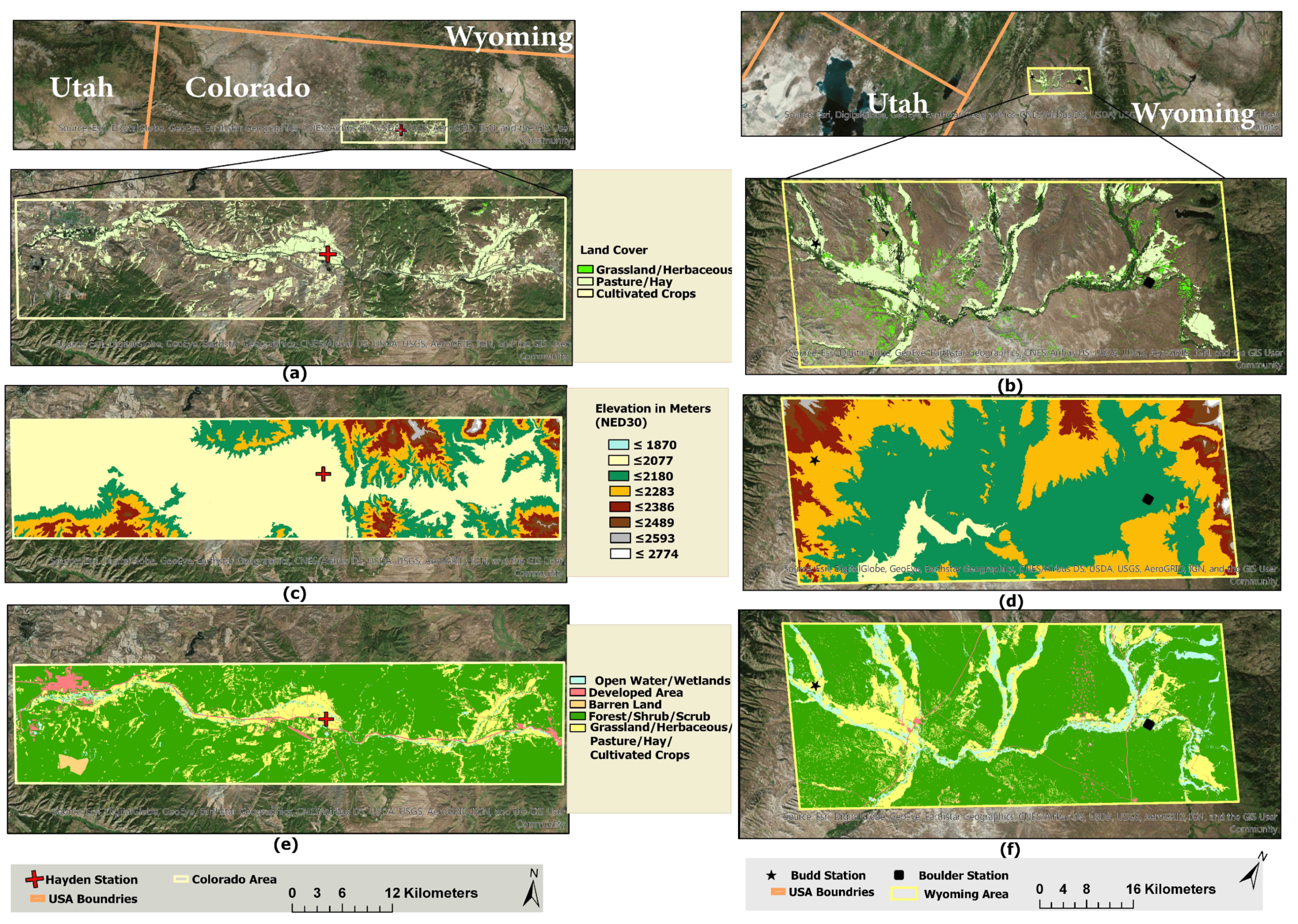
2.1. Area of Study

This research considered two study areas or locations. The first consisted of agricultural lands in a small sub-basin in Central Colorado with only one active hourly station called “Hayden, Yampa Vall”. The latitude and longitude of the weather station are 40.4833 N and 107.2166 W, respectively, at 2011 m above sea level (asl), and the study area is about 1000 km 2 . The second area of study is located in Wyoming and has two active hourly stations called “Budd” and “Boulder Rearing”. The coordinates are 42.5780 N, 110.10972 W at 2117 m asl and 42.7158 N, 109.6897 W at 2130 m asl, respectively. The distance between the two stations is 57 km, and the study area is about 2300 km 2 . The rectangular shape around these stations that is considered the area of study includes dense pasture, hay, grassland, herbaceous, and cultivated crop lands. Both Haden station in Colorado and Boulder station in Wyoming are located in plateau regions, but Budd station in Wyoming is located in a mountain region. The performance of all three spatial datasets against rain gauges was evaluated for the growing season in 2014, 2015 and 2016. The geographic location layout of these case studies and the location of weather stations with elevation and 2011 NLCD (land cover classes) [22] are shown in Figure 1.
As shown in the left column in Figure 1, the first case study located in Colorado has only one active weather station (Figure 1a) as is also shown on the MesoWest website [23]. Except for the western edges, the elevation increases from the center to the edges in a north/south direction (narrow valley). The center area toward the west has a low elevation and is almost flat (Figure 1c). The middle area is covered by grassland, herbaceous plants, pasture, and hay [22]. Most of the other hill slope locations are covered by forest (Figure 1e).
The right column of Figure 1 illustrates the geographical location of the second case study located in the Wyoming basin and its weather stations (Figure 1b), along with maps of peaks and valleys (Figure 1d). As shown in these figures, the “Boulder Rearing” station is located at a low elevation, while the “Budd” station is located at a high elevation. As in the Colorado case study, most parts of the Wyoming study area are covered by shrub, forest, and grassland. The majority of the forest lands are in the high-elevation terrain, whereas the grassland areas are in the lowlands (Figure 1f). The middle part of the Wyoming study area has lower elevations and is covered by grassland, pasture, and hay.

2.2. Precipitation Products

In this study, three data sources were used to show the importance of resolution at the farm level. These datasets are described below, and a summary of their temporal and geographical resolution and availability is presented in Table 1. The quality control of the precipitation products, as well as the weather station records was performed by other competent agencies. The same is true for the gridded datasets, such as PRISM. According to the PRISM documentation (https://developers.google.com/earth-engine/datasets/catalog/OREGONSTATE_PRISM_AN81d), the quality control of the observation network requires a comparatively long period of time. Thus, PRISM datasets are re-calculated several times until six months have elapsed. Regarding Daymet, the data provider (Oak Ridge National Laboratory) carried out the cross-validation. TRMM 3B42 is also provided by NASA along with its relative error (mm/h). Regarding the rain gauge data, we refer the interested readers to MesoWest [23] operated by the University of Utah and CoAgmet [24] operated by Colorado State University.

2.2.1. TRMM-3B42

TRMM-3B42 is an algorithm that produces precipitation data using a combination of thermal infrared data from geostationary satellite and passive microwave data from four sources: TRMM microwave imager (TMI), Special Sensor Microwave Imager (SSM/I), Advanced Microwave Sounding Unit (AMSU), and Advanced Microwave Sounding Radiometer-Earth Observing System (AMSR-E) (Huffman et al., 2007 [25]). This precipitation estimate was generated in four steps: adjusting and combining the Passive Microwave (PM) estimations, creating Thermal Infrared (TIR) precipitation estimations using adjusted and combined PM estimations, evaluating TIR precipitations, and indirectly adjusting the data using gauge observations. TRMM-3B42 is available after the end of each month at a resolution of 0.25° (∼25 km).

2.2.2. PRISM

The Precipitation-elevation Regression on Independent Slopes Model (PRISM) is an interpolation model developed at Oregon State University (Dally et al., 2007 [26], and Dally et al., 2015 [27]). PRISM provides several distributed variables on a regular grid size with different spatial and temporal resolutions (1 km and 4 km). These variables are calculated using linear relationships between climatic variables and elevation values. The factors considered in this weighted regression model are location, elevation, topographic features, vertical atmospheric layer information, coastal proximity, and terrain orographic effectiveness. Values assigned to a grid cell are calculated based on a linear regression of climate station values versus elevation. In this model, a moving-window procedure is employed to extract a unique regression function for each grid cell. Next, a specific weight is assigned to each station based on the aforementioned factors, and a climate-elevation gradient is calculated. Ultimately, an averaged center-cell value is calculated based on its neighboring values and the distance between the center grid cell and neighboring grid cells. One of the most important variables achieved by PRISM is precipitation (4 km), which is used as input information for hydrologic modeling and climatic research. After 6 complete months have passed, the datasets are considered stable, but before that time, the datasets are not finalized and are called “provisional”.

2.2.3. Daymet

This set provides gridded daily weather variables for North America. These variables are minimum and maximum temperature, precipitation, humidity, shortwave radiation, snow water equivalent, and day length. The temporal resolution of Daymet is a daily time step, and the spatial resolution is 1 km. The outputs of this model are useful in hydrology, carbon cycle science, climate change analysis, etc. This dataset is available for 1980 through the latest full calendar year for the United States, Mexico, Canada, Hawaii, and Puerto Rico (Thornton et al., 2017 [28]). Most of the time, there is a one-year latency in Daymet data availability.

2.2.4. Weather Station Data Source
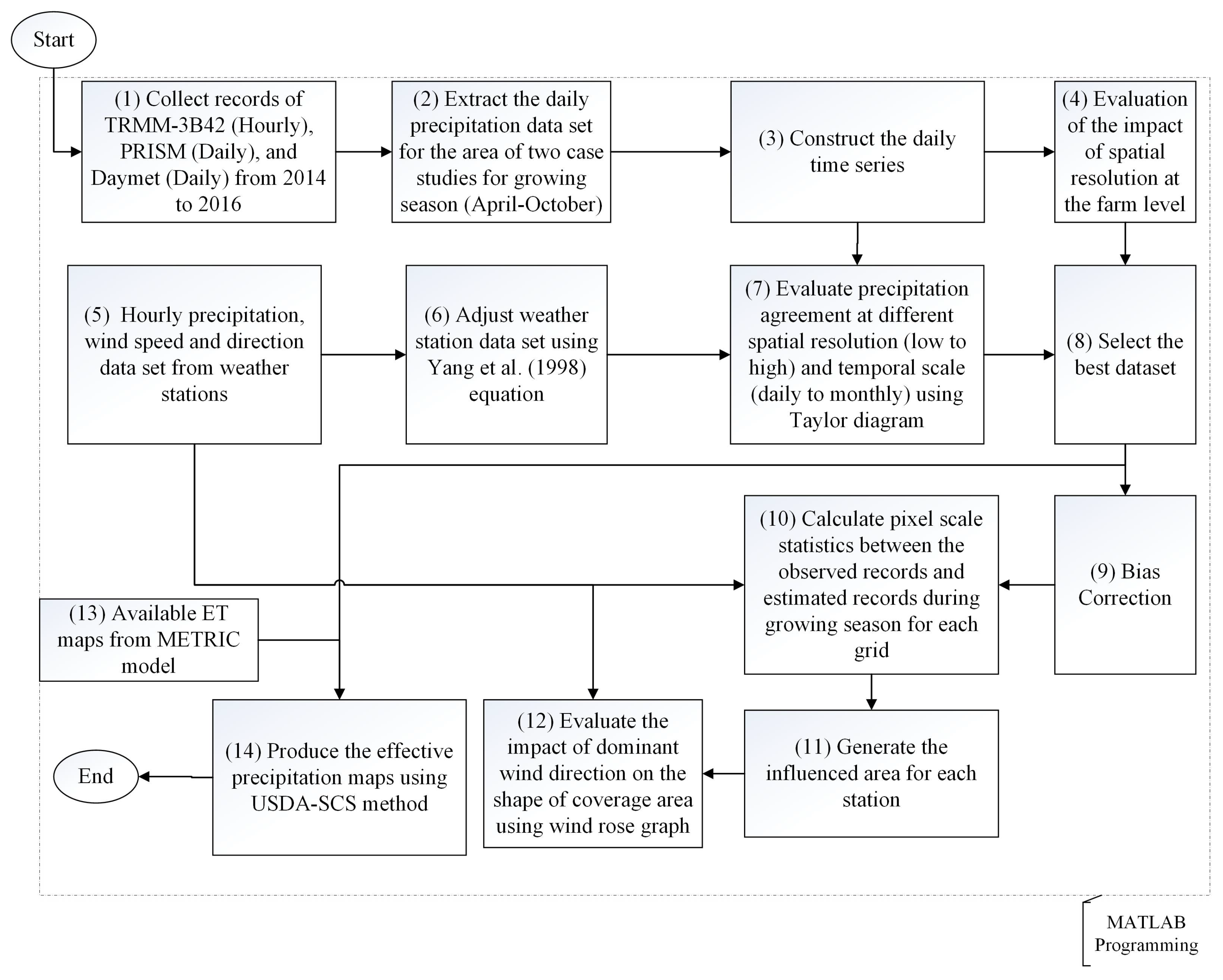
Weather station records can be obtained from several sources, such as CoAgmet [24], MesoWest [23], and Cli-Mate [29]. The precipitation records for Wyoming (Budd and Boulder stations) were provided by the Wyoming Division of Water Resources, and the records for Colorado were downloaded from the CoAgmet server [24]. For the aforementioned regions, the required information to plot wind rose graphs was not available. However, MesoWest ([23]) provides near real-time active weather station observation records in a Comma-Separated Values (CSV) format. Wind speed and wind direction were extracted from this source and used in this study. All of the gauge records that included rain, wind direction, and wind speed are provided at hourly time step by these data sources.

2.3. Methodology

The methodology of this study is presented graphically below. The analysis was performed for the growing season (April–October) as shown in Figure 2.
As illustrated in Figure 2, precipitation sources including TRMM-3B42, PRISM, and Daymet were first downloaded for 2014–2016 (Step 1). TRMM-3B42 provides 3-h time scale precipitation, whereas PRISM and Daymet are daily datasets. The datasets were clipped for the case studies and for the growing season (April–October). TRMM-3B42 precipitation values were converted to a daily scale (Step 2). In the third step, the three daily spatial time series (TRMM-3B42, PRISM, and Daymet) were constructed for each year (Step 3). Next, the impact of high-resolution spatial precipitation maps at the farm level (i.e., 30-m resolution) was evaluated by comparing the irrigated unit from NLCD 2011 [22] versus the three different precipitation products (Step 4). In Steps 5 and 6, the hourly observed rainfall, wind speed, and wind direction for the gauge station (Figure 1) were obtained and converted to a daily time step, and the rainfall records were adjusted using Equation (1) provided by Yang et al. (1998) [30]. After these adjustments, precipitation agreement at different temporal and spatial scales between all precipitation sources versus rain gauge records was examined using a Taylor diagram (Taylor, 2011 [31]) and statistical indices (Step 7). Based on the results of Steps 4 and 7, one of the spatial precipitation products was selected, and its bias from observed records was addressed (Steps 8 and 9). Because both case studies were poor in terms of the number of active stations, it was assumed that the daily bias of all sources at the gauge location was a constant value for other surrounding locations. After bias correction, the Summation of Absolute Error (SAE) during the growing season as a statistical index was calculated between the daily rainfall records of the gauge and daily precipitation of the chosen precipitation data, and then, the gauge coverage area was generated (Steps 10 and 11). In Step 12, the “wind rose” graph was drawn using the wind direction and wind speed recorded at the gauge, and the relationship between the dominant wind direction and the elongation direction of the influenced area for each station was examined. As a final step, ET maps from the METRIC model (Step 13) were used in the USDA-SCS approach, along with monthly rainfall calculated using Equation (3), to estimate effective rainfall maps (Step 14). The code for this methodology can be found at http://www.hydroshare.org/resource/591bfb4171834eb287fb6c0725d7e3dd.

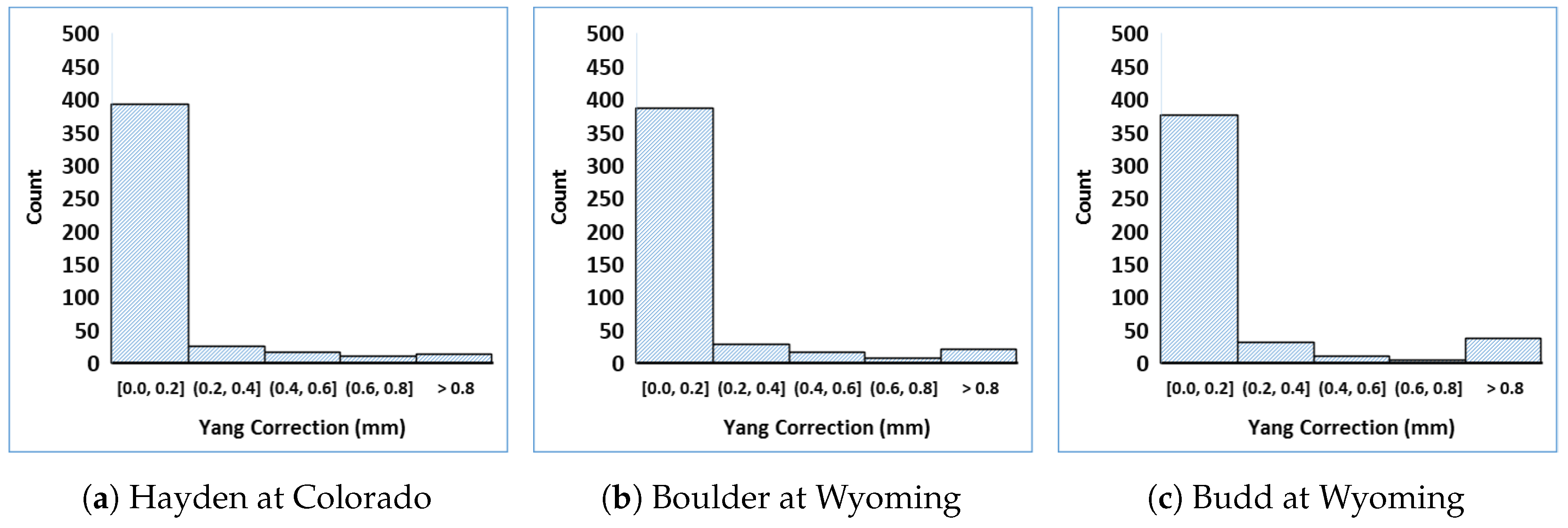
2.3.1. Yang Correction for Gauge Precipitation Data

Because of Venturi effects and evaporation, precipitation records measured by precipitation gauges are usually underestimated. To adjust these records, all of the daily rainfall gathered from the weather stations for both case studies during the growing season (1 April–1 October) of each year were adjusted by Equation (1), recommended by the World Meteorological Organization (Yang et al. 1998 [30]) based on the wind values at the weather stations. This step is necessary because the Yang adjustment is rarely performed for any weather data.
P a d j = P g a u g e ( e x p ( 0.062 × u g 0.58 ) )
in which P a d j = the adjusted precipitation (mm); P g a u g e = precipitation recorded at the weather station (mm); and u g = wind speed at the weather station (m/s).

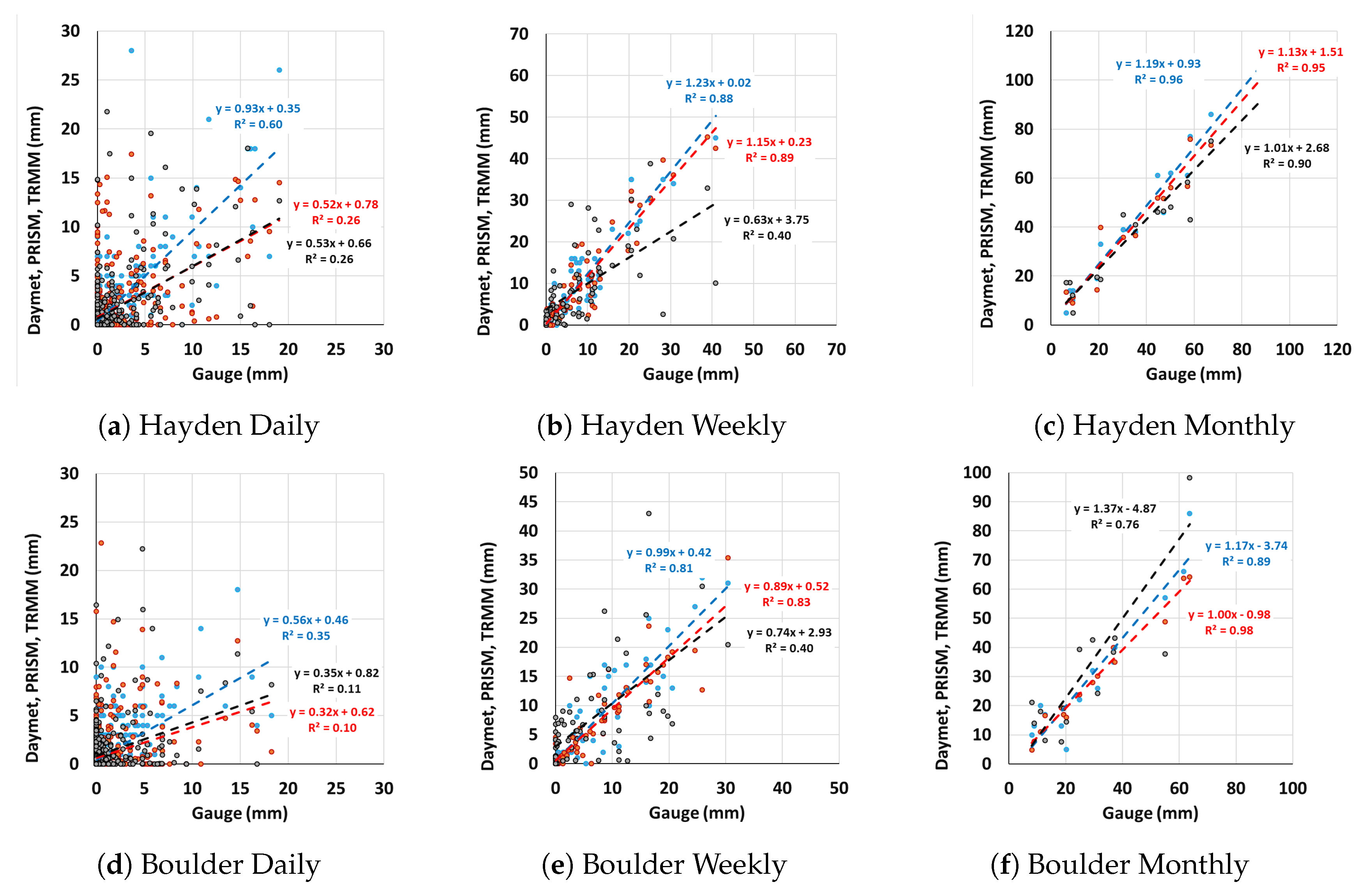
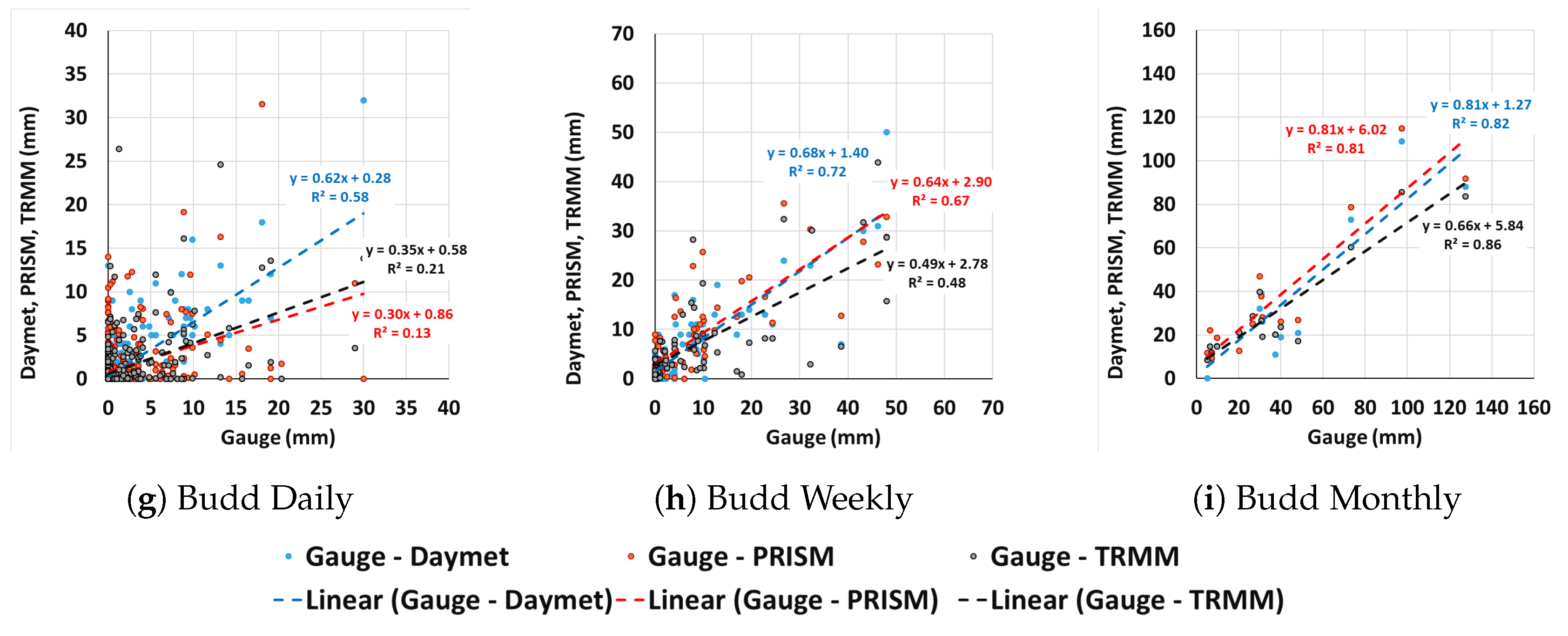
2.3.2. Bias Analysis with Statistical Indices

After adjusting rain gauge records to account for Venturi and evaporation effects, the bias of each spatial dataset versus the adjusted gauge records was examined. To do that, the time series of precipitation from the weather station versus the time series of precipitation from the pixel of the spatial datasets on which the weather station was located was evaluated at three time scales (daily, weekly, and monthly). For the evaluation, the Taylor diagram ([31]), Nash–Sutcliffe model efficiency coefficient ( N S E , Equation (6)), and Summation of Absolute Error ( S A E , Equation (7)), along with scatter plots of the gauge records versus the aforementioned datasets were used. In the Taylor diagram, three statistics are related to each other based on Equation (2): Pearson correlation coefficient ( ρ ), root-mean-squared error ( R M S E ), and standard deviation ( S D ) (Equations (3)–(5)). Therefore, this diagram can show multiple aspects of model performance in a single diagram.
E = σ e 2 + σ o 2 2 σ e σ o ρ
in which E = the centered RMSE between observations and estimations; ρ = Pearson correlation coefficient; σ o and σ e = the standard deviation of the observations and estimations, respectively.
ρ = t = 1 n ( P a d j ( t ) P a d j ¯ ) ( P s ( t ) P s ¯ ) t = 1 n ( P a d j ( t ) P a d j ¯ ) 2 t = 1 n ( P s ( t ) P s ¯ ) 2
R M S E = t = 1 n ( P s ( t ) P a d j ( t ) ) 2 n
S D = t = 1 n ( P ( t ) P ( t ) ¯ ) 2 n
in which P a d j ( t ) = the adjusted precipitation in time period t; P s ( t ) = the precipitation estimation in period t; P a d j ¯ = the average adjusted precipitation in period t; P s ¯ = the average precipitation estimation in period t; P ( t ) = the precipitation in period t; P ( t ) ¯ = the average precipitation in period t; n = the number of records.
N S E = 1 i = 1 n ( P s ( t ) P a d j ( t ) ) 2 i = 1 n ( P s ( t ) P ¯ a d j ( t ) ) 2
S A E = M A E n = i = 1 n | P s ( t ) P a d j ( t ) |
It is important to clarify the use of SAE instead of MAE in this study. While MAE provides an averaged value for the precipitation differences between the gauge station and the corresponding pixel in the precipitation dataset, SAE presents the same information, but it can be tied to the risk to the irrigator (in mm/season) using the precipitation information, depending on the distance between the field and the gauge location.

2.3.3. Bias Correction

After choosing a spatial precipitation product for further analysis in this study, it was necessary to remove the bias from estimation records based on local observations. Because these case studies were in poor regions in terms of the number of active gauge stations (1 in Colorado and 2 in Wyoming), a simple daily spatial bias correction procedure was applied on the selected dataset. For bias correction in both regions under study, the differences between daily time series of rainfall measured at the weather stations and daily time series of the selected spatial dataset were calculated and subtracted. These bias values were considered as a constant correction for each day.

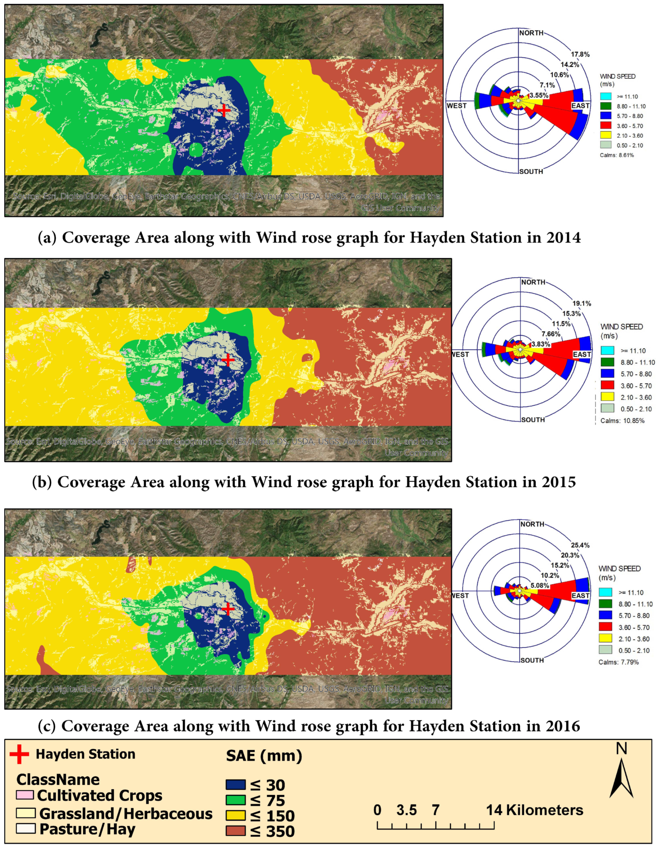
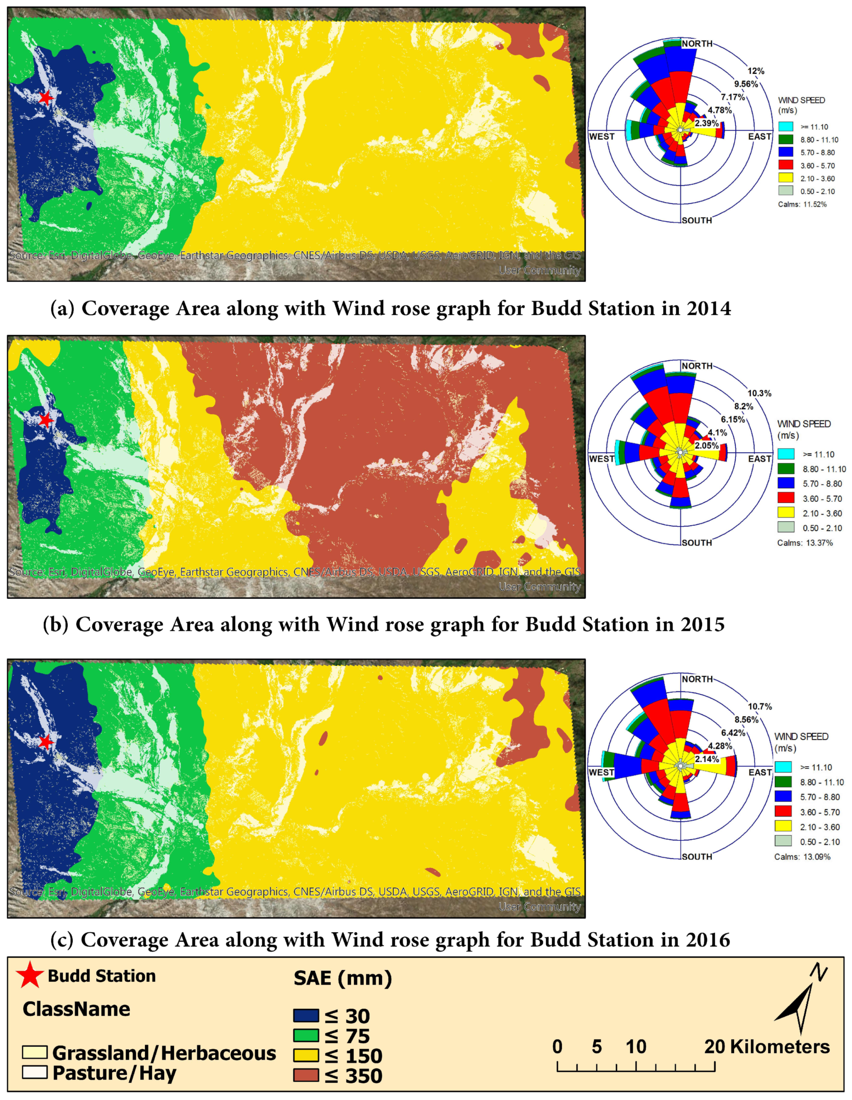
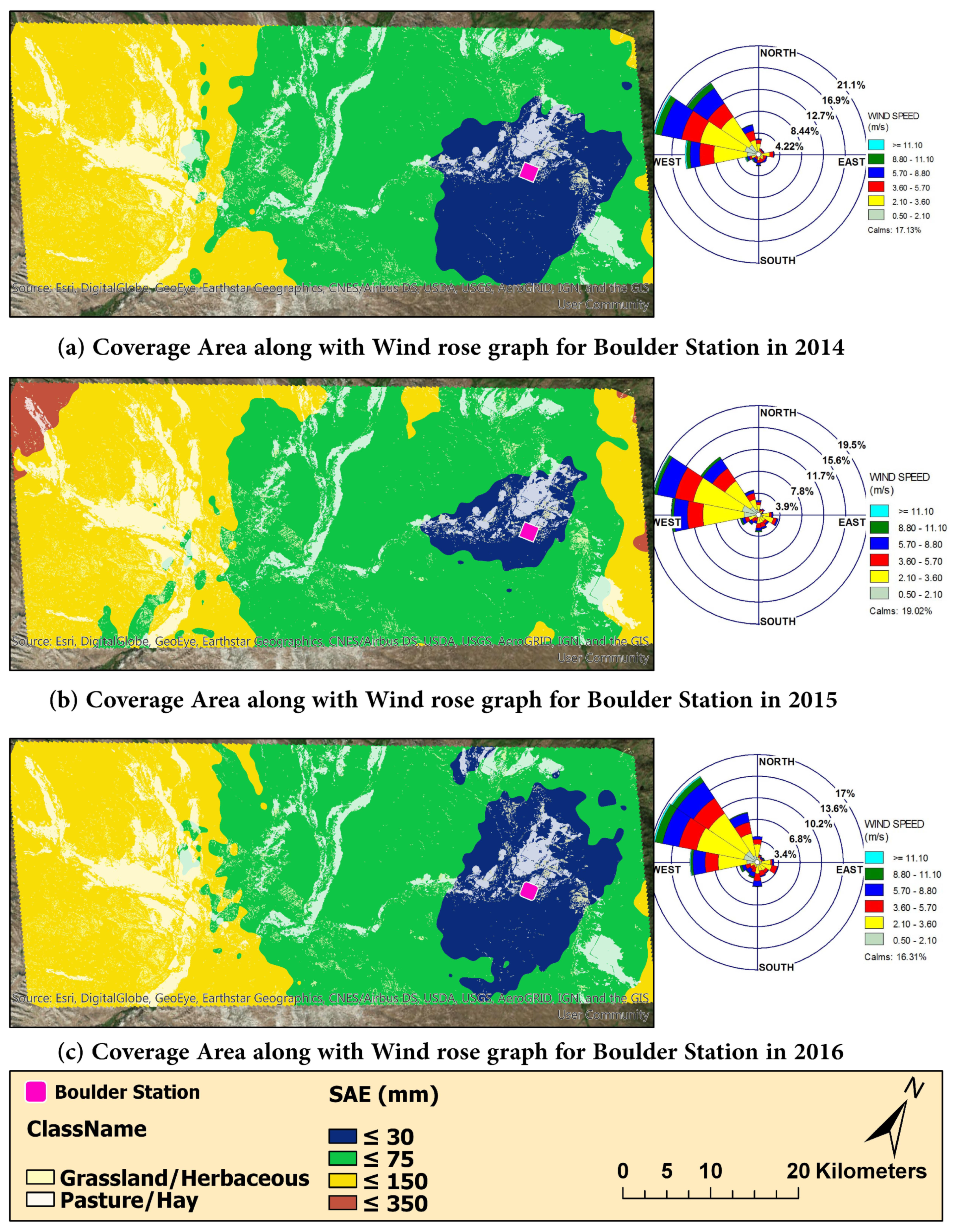
2.3.4. Gauge Coverage Area or Area of Influence

To determine the gauge coverage area, SAE using Equation (7) during the growing season between the adjusted gauge records (observations) and the bias corrected precipitation of each pixel from the selected products (estimations) was calculated and shown spatially.

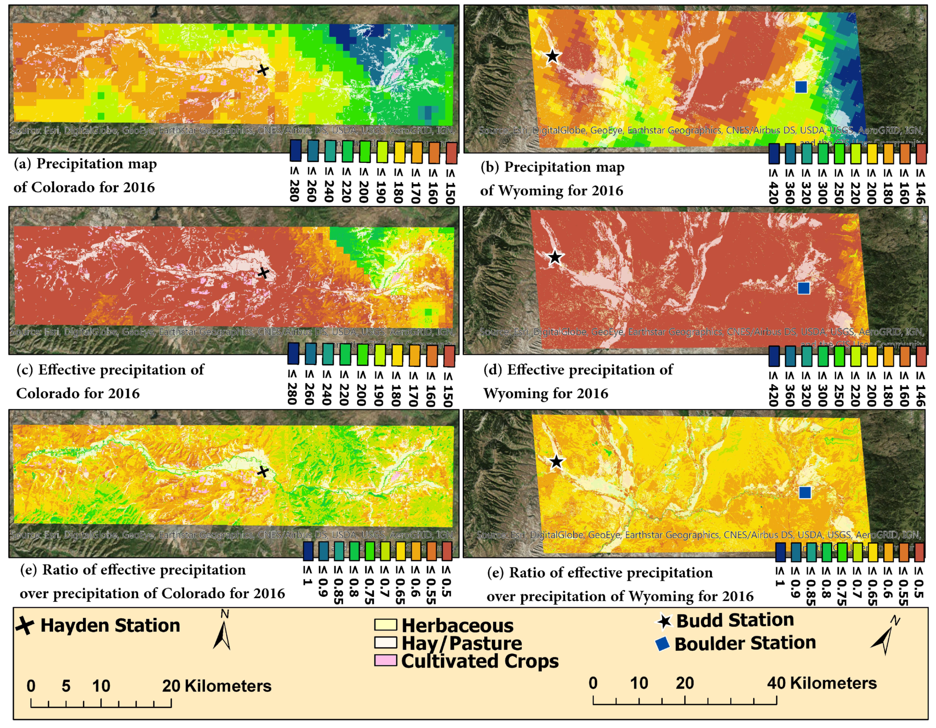
2.3.5. Effective Precipitation Using the USDA-SCS Method

Numerous methods have been presented to estimate effective rainfall. These methods can be categorized into three groups: direct measurement, modeling water balance, and empirical or semi-empirical equations [32]. In this study, due to the availability of actual spatial ET estimates, the approach proposed by the U.S. Department of Agriculture (1970) called the USDA-Soil Conservation Service (SCS) was used to determine the effective rainfall. Equations (8) and (9) were extracted based on the 50 years of rainfall records analyzed at 22 meteorological stations over the United States.
P e = S F ( 1.253 P t 0.824 2.935 ) ( 10 0.001 E T C )
S F = ( 0.531747 + 0.295164 D 0.057697 D 2 + 0.003804 D 3 )
in which P e = average monthly effective precipitation (mm/month); P t = total precipitation for the month in mm (mm/month); E T C = crop ET per month (mm/month) [33]; S F = multiplication factors that depend on net depth of irrigation (D) in inches [34]. The value of the net depth of irrigation can be estimated from Table 2 [35]. To calculate the spatial effective rainfall, it is necessary to access the monthly value of actual ET. In this study, the monthly ET maps using METRIC models from the study prepared by Allen and Torres-Rua, 2018 [36], were used. Furthermore, D = 40 mm (1.57 inches) because of the loamy soil texture of both case study areas and assuming medium rooting crops as expected for alfalfa and pasture hay. Therefore, SF is equal to 0.87, and effective rainfall for each pixel can be calculated using Equation (8).

3. Results and Discussion

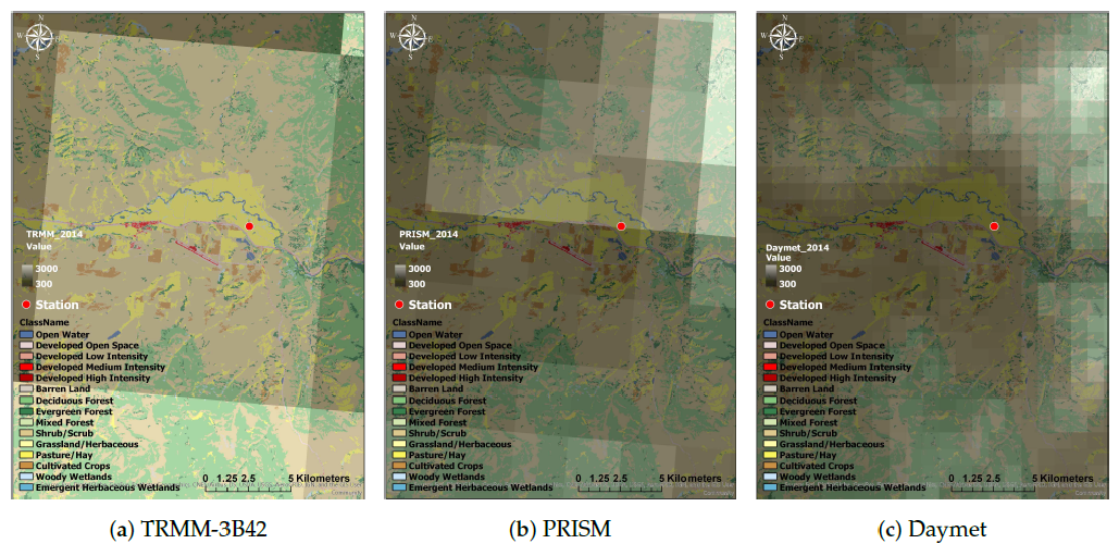
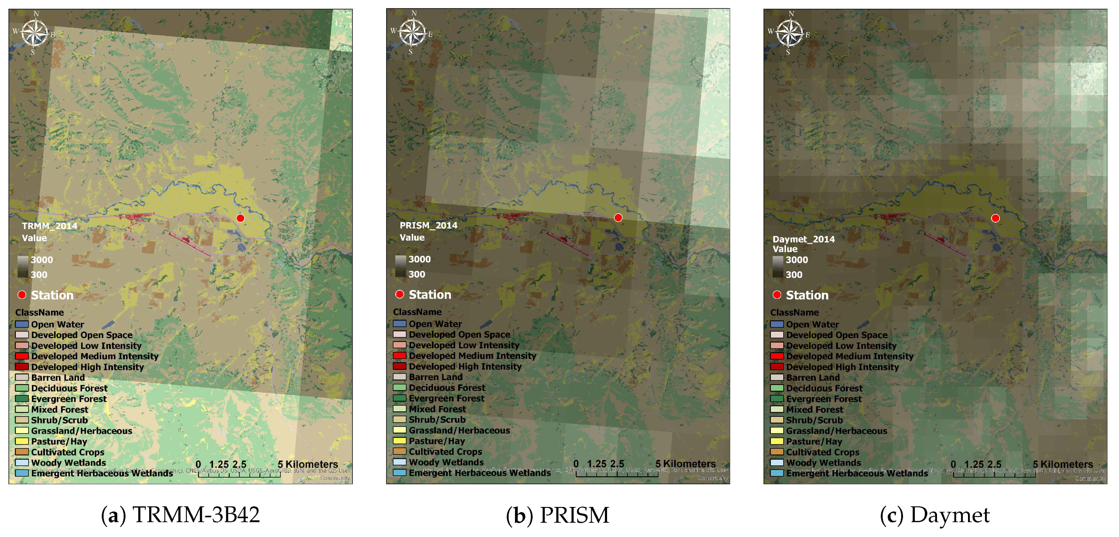
3.1. Spatial Precipitation Resolution Impact

In addition to the delay time for availability (“latency”) discussed in the precipitation products (Table 1), an important aspect of precipitation datasets is their spatial resolution. The adequacy of spatial resolution for farm units is shown in Figure 3. This figure presents the cumulative precipitation layer for 2014 from each dataset, along with the land cover layer from the National Land Cover Database (NLCD 2011 [22]) for the area around the weather station in Colorado. The NLCD is a 30-m Landsat-based land cover created by the Multi-Resolution Land Characteristics (MRLC) Consortium using a decision tree classification method. The resolution of TRMM is 0.25 degrees (∼25 km), while PRISM is 4 km, and Daymet is 1 km. It is evident that, for irrigation purposes at the farm unit, the resolution of TRMM and PRISM will not provide useful information. The TRMM pixel located on the weather station has a high degree of aggregation that becomes non-representative of terrain elevation or other factors influencing the weather station. Although a higher resolution of precipitation data is desired, Daymet resolution seems to be enough for the average American farm, which is 435 acres or 1.7 km 2 (USDA, 2012 [37]).

3.2. Yang Correction

After assessing the importance of high-resolution rainfall datasets at the farm level, it is necessary to compare the estimation records with the observed records in terms of their accuracy. However, before making this comparison, the gauge records need to be adjusted because of Venturi effects and evaporation. The histogram of differences between precipitation gauges before and after adjustment based on the Yang correction is shown in Figure 4.
Figure 4 indicates that the Yang correction adjustment needed on the precipitation recorded at the stations is about 0.1 mm/day. However, on windy days, the Venturi effect and evaporation were larger. On those days, the difference was greater than 0.8 mm/day, particularly at Budd station in Wyoming, which is located at a high elevation (2117 m asl).

3.3. Spatial Precipitation Bias Analysis

Figure 5 presents the performance of several aspects of each dataset ( ρ , RMSE, and SD) using the Taylor diagram after the Yang correction. The Taylor diagram is a graph facilitating the comparative assessment of three statistical indices (Pearson correlation coefficient, root-mean-squared error, and the standard deviation) calculated between observed records and modeled values for a specific variable or parameter. The Taylor diagram can summarize the accuracy of all three datasets versus observations using the aforementioned indices simultaneously (Ghajarnia et al. [38]). This figure illustrates the results of the Taylor diagram at different time scales (daily, weekly, monthly).
In terms of the effect of temporal resolution (daily, weekly, monthly), the monthly scale showed a stronger correlation between precipitation products and gauge records in terms of ρ than the weekly or daily scale. This might originate from the impact of aggregation on outliers. In upscaling, errors at higher resolution scales (in terms of both temporal and spatial resolution) will be indemnified, to some extent (Ren et al., 2018 [39], and Zhang et al., 2018 [40]). For example, the correlation of ρ between TRMM and the gauge for all three stations at the daily scale was about 0.5, while at the monthly scale, it increased to 0.90. This pattern held for PRISM and Daymet, with the correlation of PRISM vs. gauge and Daymet vs. gauge increasing from 0.4–0.95 and 0.7–0.97, respectively. The R M S E of TRMM was ∼3 mm/day, 7–9 mm/week, and 10–15 mm/month; and the R M S E of both PRISM and Daymet was ∼2.5 mm/day, 3–7 mm/week, and 4–15 mm/month. Furthermore, Daymet outperformed PRISM at all daily, weekly, and monthly scales, and PRISM performed better than TRMM at the monthly scale. In general, the accuracy of Daymet and PRISM were similar, and decreasing the temporal resolution led to an improved relationship between the estimation records (TRMM, Daymet, and PRISM) and observations (gauge).
The N S E and S A E reported in Table 3 and the scatter plots shown in Figure 6 are useful for assessing the performance of the spatial precipitation versus the gauge records. According to Table 3, the performance of all datasets versus the observations was acceptable in terms of N S E , except for the estimation records at the daily scale and estimation of TRMM at both daily and weekly scales. In terms of SAE, the performances of TRMM and Daymet at the daily scale were similar (between 400 and 500 mm/day). However, when the temporal resolution decreased, the performances of Daymet and PRISM were similar. To summarize, Daymet and PRISM, as provided online, can be considered adequate only at weekly and monthly scales, and the TRMM dataset could not be considered an accurate source at either the daily or weekly scale. In other words, Table 3 reveals that, even though N S E is close to 1.0 for most of the situations at weekly and monthly scales, there is a considerable disagreement with gauge records (i.e., more than 100 mm during the growing season), which could have a significant impact on farmers’ decisions for irrigation management.
Figure 6 illustrates the impact of different time scales on the spatial precipitation. In general, the correlation of Daymet with the gauge records was stronger than PRISM, and the correlation of PRISM with the gauge was stronger than TRMM, which agrees with the Taylor diagram results. Decreasing the temporal resolution also decreased the uncertainties between the spatial precipitation datasets versus the observations. Moving from daily to monthly scale, the difference in terms of trend lines between Daymet, PRISM, and TRMM-3B42 was insignificant, and those lines were similar to one another.

3.4. Weather Station Coverage Area for Rainfall

Despite latency, spatial resolution, and the disagreement of spatial precipitation products with gauge stations, these datasets, particularly Daymet, can be used to for estimation of weather station coverage area maps, assuming that the disagreement between the spatial precipitation dataset and the gauge station is removed. For this study, the disagreement (or bias) was removed in the Daymet dataset at a daily scale, assuming the disagreement was constant for the day across the areas of study. The estimation can be based on a comparison of indices such as ρ , R M S E , and N S E from the gauge time series and the time series of each Daymet pixel. However, from the perspective of irrigators and farmers, this map should clearly indicate the risk of inaccurate data due to the distance of the gauge location, with meaningful units, when they use station records for irrigation management. For xample, if they use the gauge records, they need to know the seasonal difference in precipitation for their farms during the growing season. Therefore, S A E is more adequate as a fundamental statistic (baseline) for producing the coverage area of the weather station. In addition, the pattern of the coverage area maps would be expected to be correlated to the seasonal dominant wind direction. To evaluate this assumption, the wind rose graphs of the gauge were plotted by “WRPLOT VIEW” [41] software and are shown in Figure 7, Figure 8 and Figure 9 for the three gauge stations included in this study.
Figure 7, Figure 8 and Figure 9 provide a visual approximation of the weather station coverage areas in terms of rainfall for the growing season each year (2014, 2015, 2016) along with the wind rose graphs. The wind rose graphs were plotted using wind direction and wind speed for the growing season. To follow the SAE on a spatial scale, the pasture/hay, grassland/herbaceous, and cultivated crop areas were extracted from NLCD 2011 [22] and mapped over these figures (pale color). These figures show that the gauge coverage area was affected by the selected SAE threshold and was not a fixed radius or area; it had a different area and shape in every season. The thresholds proposed in Figure 7, Figure 8 and Figure 9 were based on what an irrigator or farmer in the U.S. might choose. For example, an irrigator dependent on rainfall as an irrigation water source, or using a pressurized irrigation system, or with reduced access to water shares would prefer a small SAE (less than 0.25 ft or 75 mm) in the season, which would reduce the area of influence of the gauge station to near proximity (or require installing a weather station close to farms). Furthermore, considering the SAE threshold of 150 mm for Hayden in Colorado and Budd in Wyoming indicates that the weather station coverage area was influenced by wind direction and that the area changed depending on the year. The Boulder station in Wyoming was also influenced by wind direction, but the coverage area seemed constant in the three years evaluated. Therefore, elevation and topographic configuration will play an important role in determining gauge area of coverage. In terms of SAE, 150 mm (1/2 ft) could be a reasonable risk threshold for farmers beyond which the weather station records cannot be considered reliable. With this threshold, there may not be a need for additional stations for Wyoming (when combining Figure 8 and Figure 9). In addition, for each pixel, these maps can show which weather station should have the higher priority to be used. In contrast, the single Colorado station was not enough to cover that study area. As shown in Figure 7, the performance of the station could be adequate for the farm units located in the western part of the study area, but not in the eastern and northeastern parts. Another important aspect of these figures is the relationship between the dominant wind direction and the elongation of the weather station coverage areas. This relationship is more pronounced for the Colorado and Budd stations. In Colorado, the dominant wind was blowing from east to west and in Budd was blowing from north to south. For both stations, the elongation of the influence area was compatible with wind direction patterns.

3.5. Spatial Effective Rainfall Estimates

The evaluation of the Daymet dataset in this study revealed that its performance was acceptable at the monthly scale. Thus, if monthly ET maps are available, the methodology proposed by USDA-SCS can be used to estimate effective rainfall, which would be more desirable for irrigators and farmers. Since ET maps from METRIC, using Landsat imagery at 30-m resolution, are available for the areas of study, the effective rainfall estimates can be achieved using ET (at 30-m resolution) and a resampled version of Daymet (from 1 km–30 m). To resample Daymet, a simple resampling tool in the ArcGIS resampling toolbox was used with a “nearest” method. Thus, the resolution of the effective rainfall in Figure 10 was 30 m. Since the differences between the rainfall and effective rainfall were related to runoff and deep percolation, the Ratio of Effective precipitation over precipitation (REP) showed how much of the seasonal rainfall was stored in the root zone to be used by the crops. Therefore, the information from the REP maps can provide essential information for irrigators and farmers in terms of decisions about supplemental irrigation. Figure 10 shows the precipitation, effective precipitation, and REP of both the Colorado and Wyoming regions for the 2016 growing season.
As illustrated in the left column in Figure 10, the amount of precipitation extracted from Daymet for the 2016 growing season in the Colorado region ranged from 146 mm–412 mm (Figure 10a). However, some part of this precipitation will be stored in the soil as effective precipitation, ranging from 77 mm–321 mm (Figure 10c). Although the pattern of precipitation and effective precipitation was quite similar, the REP was not a constant value for the entire study area. According to Figure 10e, REP for agricultural units in 2016 was about 65%, which means that up to 65% of the seasonal precipitation successfully infiltrated the root zone and 35% was lost through deep percolation and run-off. Since the USDA-SCS approach was developed only for agricultural fields, the REP values for non-agricultural units cannot be considered accurate. As in the Colorado region, the spatial pattern of precipitation and effective precipitation in the Wyoming region were similar to one another, and the amounts of precipitation and effective precipitation were 137 mm–277 mm and 71 mm–247 mm, respectively. Again, in the Wyoming region, almost 65% of the seasonal precipitation can be considered as effective rainfall.
While this study presents the effective rainfall analysis at seasonal scale, two major factors influence its accuracy and stability: (a) Daymet accuracy at the monthly scale was assumed to be adequate, and evaluation and correction of Daymet data requires additional (nonexistent) gauge stations, which is beyond the scope and objective of this study; and (b) given that rainfall is stochastic in nature, within a growing season, some months can be wetter or drier than the historical monthly pattern, and the accuracy and stability are influenced by the season (wetter years). Thus, a more detailed analysis of monthly effective precipitation using USDA-SCS implies the disaggregation of the analysis done in this study at the monthly scale and spatial estimation the multiplication factor based on soil type and crop root size.

4. Summary and Conclusions

Rainfall plays an important role in water resources management; thus, its adequate quantification helps water managers, irrigators, and farmers to have a significant impact on water efficiency. In this study, precipitation data (as gauge or spatial datasets) were evaluated on their adequacy for use as sources of information for agricultural water management at the farm scale. All evaluated spatial precipitation products (TRMM-3B42, PRISM and Daymet) had disagreement with gauge station data. Spatial and temporal resolution, along with data latency, were other limitations for field- and farm-level analysis. Thus, observed rainfall records obtained from gauges are the most reliable and real-time accessible data. However, because of the distance from the gauge, these records may not be applicable for specific farms. Distance to weather stations, topography, wind direction, wind speed, and the value and frequency of precipitation can all affect the coverage area of the weather stations. Therefore, maps that show the coverage area are essential for farmers and water managers. In this study, the coverage area of weather stations located in two different regions in the Upper Colorado River Basin (Colorado and Wyoming regions) for 2014, 2015, and 2016 were estimated using a statistical approach based on gauge records, remote sensing data, and gridded climate data in terms of rainfall and effective rainfall. To select the proper precipitation datasets, the records of the gauges were adjusted and then compared to one another based on the spatial resolution of the farms and their agreement with observed records using the Taylor diagram. Daymet was selected as the proper dataset; its bias was corrected, and the coverage area of the stations was determined based on the SAE between the corrected Daymet and the gauge records. In addition, the shape of the coverage area was compared to the dominant wind direction using wind rose diagrams. Finally, the USDA-SCS method was used to generate the effective rainfall on a spatial scale utilizing available monthly ET maps derived from the METRIC model and monthly precipitation from Daymet.
The results revealed that decreasing the temporal resolution or intervals (daily to monthly) and increasing the spatial resolution (TRMM to Daymet) increases the agreement of the spatial datasets (estimations) to the gauge (observations). Furthermore, PRISM and Daymet were similar in performance and were better than TRMM. However, all three datasets showed significant bias from observations on a daily and weekly scale in terms of SAE, despite their acceptable performance in terms of NSE. Results showed that, although the pattern of the coverage area for each of the stations was nearly consistent during the study years (2014–2016), the extent of that areas was not constant. In terms of coverage area based on rainfall, the dominant wind direction could be related to the elongated shape of the coverage area. However, no definitive pattern emerged between the wind factor and the extent of the area of influence. Regarding the risk level thresholds for disagreement in rainfall values, the gauges in Wyoming were shown to cover significant portions of the study area, but data users should pay attention to the coverage extent of each station. In contrast, the gauge located in the Colorado region covers only the western area around its location. Therefore, the records from this station cannot provide a reliable estimation for the eastern side of the gauge in this study area. The technique used in this study has the potential to be used in determining optimal or near-optimal additional gauge locations while maximizing the coverage area as an objective function. Future work could evaluate factors that affect the fluctuation of the coverage area. Since Daymet had acceptable agreement with the gauge records at the monthly scale and had a higher spatial resolution, it can be consider as a useful spatial rainfall source to produce spatial maps of loss (run-off and deep percolation) using effective rainfall methods (direct measurements, water balance models, statistical models). Providing the effective rainfall maps at this temporal and spatial scale not only is important for water resources managers, but is useful for irrigators. However, one-year latency in Daymet data availability is a challenge for a real-time field irrigation scheduling. The analysis of effective precipitation using the USDA-SCS approach revealed that in most agricultural areas, up to 65% of the seasonal precipitation can be stored in the soil to be used by the crops, and about 35% will be lost through run-off and deep percolation processes.

Author Contributions

M.A. and A.F.T.-R. conceived of and designed the experiments; M.A. performed the experiments; M.A. and A.F.T.-R. analyzed the data; N.A. and A.F.T.-R. contributed reagents/materials/analysis tools; M.A. wrote the paper.

Funding

This project was financially supported by the Utah Water Research Laboratory at Utah State University. The project was also partially funded by the Walton Family Foundation and SD Betchel Foundation.

Acknowledgments

The authors would like to thank Carri Richards for editing the manuscript and also to anonymous reviewers for improving the paper by providing constructive comments.

Conflicts of Interest

The authors declare no conflict of interest.

Abbreviations

The following abbreviations are used in this manuscript:
SGMSatellite-Gauge-Model
GPCCGlobal Precipitation Climatology Center
1DDOne-Degree Daily
GPCPGlobal Precipitation Climatology Project
TRMMTropical Rainfall Measuring Mission
CONUSContiguous United States
GHCN-DGlobal Historical Climatology Network-Daily
PRISMParameter-Elevation Regression on Independent Slopes Model
PERSIANNPrecipitation Estimation from Remotely-Sensed Information using Artificial Neural Networks
ANNArtificial Neural Network
IDWInverse Square Distance Weighting
KEDKriging with the External Drift
ETEvapotranspiration
TMITRMM microwave imager
SSM/ISpecial Sensor Microwave Imager
AMSUAdvanced Microwave Sounding Unit
AMSR-EAdvanced Microwave Sounding Radiometer-Earth Observing System
PMPassive Microwave
TIRThermal Infrared
NLCDNational Land Cover Database
SAESummation of Absolute Error
RMSERoot-Mean-Squared Error
SDStandard Deviation
NSENash–Sutcliffe model Efficiency
USDAU.S. Department of Agriculture
SCSSoil Conservation Service
MRLCMulti-Resolution Land Characteristics
CMAPThe Climate Prediction Center Merged Analysis of Precipitation
REPThe Ratio of Effective precipitation over Precipitation

References

  1. Huffman, G.J.; Adler, F.R.; Rudolf, B.; Schneider, U.; Keehn, P.R. Global precipitation estimates based on a technique for combining satellite-based estimates, rain gauge analysis, and NWP model precipitation information. J. Clim. 1994, 8, 1284–1295. [Google Scholar] [CrossRef]
  2. Xie, P.; Arkin, P. Analyses of global monthly precipitation using gauge observations, satellite estimates, and numerical model predictions. J. Clim. 1995, 9, 840–855. [Google Scholar] [CrossRef]
  3. Huffman, G.J.; Adler, F.R.; Morrissey, M.M.; Bolvin, D.T.; Curtis, S.; Joyce, R.; McGavock, B.; Susskind, J. Global precipitation at one-degree daily resolution from multisatellite observations. J. Hydrometeorol. 2000, 2, 36–50. [Google Scholar] [CrossRef]
  4. Adler, F.R.; Huffman, G.J.; Bolvin, D.T.; Curtis, S.; Nelkin, E.J. Tropical Rainfall Distributions Determined Using TRMM Combined with Other Satellite and Rain Gauge Information. J. Appl. Meteorol. Climatol. 2000, 39, 2007–2023. [Google Scholar] [CrossRef] [Green Version]
  5. Yatagai, A.; Arakawa, O.; Kamiguchi, K.; Kawamoto, H.; Nodzu, M.I.; Hamada, A. A 44-year daily gridded precipitation dataset for Asia based on a dense network of rain gauges. Sci. Online Lett. Atmos. 2009, 5, 137–140. [Google Scholar] [CrossRef]
  6. Yatagai, A.; Kamiguchi, K.; Arakawa, O.; Hamada, A.; Yasutomi, N.; Kitoh, A. APHRODITE: Constructing a long-term daily gridded precipitation dataset for Asia based on a dense network of rain gauges. Bull. Am. Meteorol. Soc. 2012, 93, 1401–1415. [Google Scholar] [CrossRef]
  7. Prat, O.P.; Nelson, B.P. Evaluation of precipitation estimates over CONUS derived from satellite, radar, and rain gauge datasets at daily to annual scales (2002–2012). Hydrol. Earth Syst. Sci. 2015, 19, 2037–2056. [Google Scholar] [CrossRef]
  8. Austin, P.M. Relation between measured radar reflectivity and surface rainfall. Mon. Weather Rev. 1987, 115, 1053–1069. [Google Scholar] [CrossRef]
  9. Joss, J.; Lee, R. The application of radar-gauge comparison to operational profile corrections. J. Appl. Meteorol. 1995, 34, 2612–2630. [Google Scholar] [CrossRef]
  10. Sorooshian, S.; Hsu, K.; Gao, X.; Gupta, H.V.; Imam, B.; Braithwaite, D. Evaluation of PERSIANN system satellite-based estimates of tropical rainfall. Bull. Am. Meteorol. Soc. 2000, 81, 2035–2046. [Google Scholar] [CrossRef]
  11. Dinku, T.; Ceccato, P.; Grover-Kopec, E.; Lemma, M.; Connor, S.J.; Ropelewski, C.F. Validation of satellite rainfall products over East Africa’s complex topography. Int. J. Remote Sens. 2007, 28, 1503–1526. [Google Scholar] [CrossRef]
  12. Su, F.; Hong, Y.; Lettenmaier, D.P. Evaluation of TRMM Multisatellite Precipitation Analysis (TMPA) and Its Utility in Hydrologic Prediction in the La Plata Basin. J. Hydrometeorol. 2008, 9, 622–640. [Google Scholar] [CrossRef]
  13. Salio, P.; Hobouchian, M.P.; Skabar, Y.G.; Vila, D. Evaluation of high-resolution satellite precipitation estimates over southern South America using a dense rain gauge network. Atmos. Res. 2015, 163, 146–161. [Google Scholar] [CrossRef]
  14. Gao, Y.C.; Liu, M.F. Evaluation of high-resolution satellite precipitation products using rain gauge observation over Tibetan Plateau. Hydrol. Earth Syst. Sci. 2013, 17, 837–849. [Google Scholar] [CrossRef]
  15. Liu, M.; Xu, X.; Sun, A.Y.; Wang, K.; Yue, Y.; Tong, X.; Liu, W. Evaluation of high-resolution satellite rainfall products using rain gauge data over complex terrain in southwest China. Theor. Appl. Climatol. 2015, 119, 203–219. [Google Scholar] [CrossRef]
  16. Chen, S.; Liu, H.; You, Y.; Mullens, E.; Hu, J.; Yuan, Y.; Huang, M.; He, L.; Luo, Y.; Zeng, X. Evaluation of high-resolution precipitation estimates from satellites during July 2012 Beijing flood event using dense rain gauge observations. PLoS ONE 2014, 9. [Google Scholar] [CrossRef] [PubMed]
  17. Lolli, S.; D’Adderio, L.; Campbell, J.R.; Sicard, M.; Welton, E.J.; Binci, A.; Rea, A.; Tokay, A.; Comerón, A.; Barragan, R.; et al. Vertically resolved precipitation intensity retrieved through a synergy between the ground-based NASA MPLNET Lidar network measurements, surface disdrometer datasets and an analytical model solution. Remote Sens. 2018, 10, 1102. [Google Scholar] [CrossRef]
  18. Buytaert, W.; Celleri, R.; Willems, P.; Bievre, B.; Wyseure, G. Spatial and temporal rainfall variability in mountainous areas: A case study from the south Ecuadorian Andes. J. Hydrol. 2006, 329, 413–421. [Google Scholar] [CrossRef] [Green Version]
  19. Haberlandt, U. Geostatistical interpolation of hourly precipitation from rain gauges and radar for a large-scale extreme rainfall event. J. Hydrol. 2007, 332, 144–157. [Google Scholar] [CrossRef]
  20. Schmidli, J.; Frei, C. Trends of heavy precipitation and wet and dry spells in Switzerland during the 20th century. Int. J. Climatol. 2005, 25, 753–771. [Google Scholar] [CrossRef] [Green Version]
  21. United States Department of Agriculture. Irrigation Water Requirements, Technical Release; United States Department of Agriculture: Washington, DC, USA, 1967; Volume 21.
  22. Homer, C.G.; Dewitz, J.A.; Yang, L.; Jin, S.; Danielson, P.; Xian, G.; Coulston, J.; Herold, N.D.; Wickham, J.D.; Megown, K. Completion of the 2011 National Land Cover Database for the conterminous United States-Representing a decade of land cover change information. Photogramm. Eng. Remote Sens. 2015, 81, 345–354. [Google Scholar]
  23. Available online: https://mesowest.utah.edu/ (accessed on 18 December 2018).
  24. Available online: https://coagmet.colostate.edu/ (accessed on 18 December 2018).
  25. Huffman, G.J.; Adler, R.F.; Bolvin, D.T.; Gu, G.; Nelkin, E.J.; Bowman, K.P.; Hong, Y.; Stocker, E.F.; Wolff, D.B. The TRMM Multi-satellite Precipitation Analysis: Quasi-Global, Multi-Year, Combined-Sensor Precipitation Estimates at Fine Scale. J. Hydrometeorol. 2007, 8, 38–55. [Google Scholar] [CrossRef]
  26. Daly, C.; Halbleib, M.; Smith, J.I.; Gibson, W.P.; Doggett, M.K.; Taylor, G.H.; Curtis, J.; Pasteris, P.A. Physiographically-sensitive mapping of temperature and precipitation across the conterminous United States. Int. J. Climatol. 2008, 28, 2031–2064. [Google Scholar] [CrossRef]
  27. Daly, C.; Smith, J.I.; Olson, K.V. Mapping atmospheric moisture climatologies across the conterminous United States. PLoS ONE 2015, 10. [Google Scholar] [CrossRef] [PubMed]
  28. Thornton, P.E.; Thornton, M.M.; Mayer, B.W.; Wei, Y.; Devarakonda, R.; Vose, R.S.; Cook, R.B. Daymet: Daily Surface Weather Data on a 1-km Grid for North America; Version 3; ORNL DAAC: Oak Ridge, TN, USA, 2017. [Google Scholar] [CrossRef]
  29. Available online: https://mrcc.illinois.edu/CLIMATE/ (accessed on 18 December 2018).
  30. Yang, D.; Goodison, B.E.; Ishida, B.; Benson, C.S. Adjustment of daily precipitation data at 10 climate stations in Alaska: Application of World Meteorological Organization intercomparison results. Water Resour. Res. 1998, 34, 241–256. [Google Scholar] [CrossRef] [Green Version]
  31. Taylor, K.E. Summarizing multiple aspects of model performance in a single diagram. J. Geophys. Res. 2001, 106, 7183–7192. [Google Scholar] [CrossRef] [Green Version]
  32. Ali, M.H.; Mubarak, S. Effective rainfall calculation methods for field crops: An Overview, Analysis and New Formulation. Asian Res. J. Agric. 2017, 7, 1–12. [Google Scholar] [CrossRef]
  33. Bos, M.G.; Kselik, R.A.L.; Allen, R.G.; Molden, D.J. Water Requirements for Irrigation and the Environment; Springer Science and Business Media: Dordrecht, The Netherlands, 2009; Chapter 3; pp. 81–102. [Google Scholar]
  34. Martin, D.L.; Gilley, J.R. National Engineering Handbook; United States Department of Agriculture (USDA), Soil Conservation Service: Washington, DC, USA, 1993; Part 623, Chapter 2; pp. 142–154.
  35. Brouwer, C.; Prins, K.; Heibloem, M. Irrigation Water Management: Irrigation Scheduling; Training Manual No. 4; FAO: Rome, Italy, 1989. [Google Scholar]
  36. Allen, L.; Torres-rua, A. Verification of Water Conservation from Deficit Irrigation Pilot Project in the Upper Colorado River Basin; Walton Family Foundation: Sacramento, CA, USA, May 2018. [Google Scholar]
  37. USDA NASS. Census of Agriculture; USDA NASS: Washington, DC, USA, 2012.
  38. Ghajarnia, N.; Liaghat, A.; Arasteh, P.D. Comparison and evaluation of high resolution precipitation estimation products in Urmia Basin-Iran. Atmos. Res. 2015, 158, 50–65. [Google Scholar] [CrossRef]
  39. Ren, P.; Li, J.; Feng, P.; Guo, Y.; Ma, Q. Evaluation of multiple satellite precipitation products and their use in hydrological modelling over the Luanhe River basin, China. Water 2018, 10, 677. [Google Scholar] [CrossRef]
  40. Zhang, Y.; Li, Y.; Ji, X.; Luo, X.; Li, X. Evaluation and hydrologic validation of three satellite-based precipitation products in the upper catchment of the Red River basin, China. Remote Sens. 2018, 10, 1881. [Google Scholar] [CrossRef]
  41. Lakes Environmental Software. WRPLOT View—Air Dispersion Modelling; Lakes Environmental Software: Waterloo, ON, Canada, 2014; Available online: http://www.WebLakes.com/ (accessed on 18 December 2018).
Figure 1. (First row) World imagery and general information of weather station locations for 1st (left column) and 2nd case study (right column); (a,b): NLCD 2011 [22] agricultural land use; (c,d): elevation map using NED (The National Elevation Dataset) 1 arc-second dataset from the USGS National Elevation Dataset program; and (e,f): land use map using NLCD 2011 [22].
Remotesensing 10 02058 g001
Figure 2. Methodology followed in the present study.
Remotesensing 10 02058 g002
Figure 3. Example of the spatial resolution of (a) TRMM-3B42, (b) PRISM, and (c) Daymet over agricultural fields in Hayden, Colorado in 2014.
Remotesensing 10 02058 g003
Figure 4. Histogram of differences between precipitation recorded at each gauge for all three seasons (2014–2016), before and after correction using Equation (1) for (a) Hayden weather station in Colorado, (b) Boulder weather station; (c) Budd weather station in Wyoming.
Remotesensing 10 02058 g004
Figure 5. (a)–(i): Taylor diagram for three spatial precipitation product versus gauge records during the growing season at different time scales for all three years, with STD and RMSE in mm/time units (mm/day, mm/week, mm/month) per column, respectively.
Remotesensing 10 02058 g005
Figure 6. Scatter plots of three spatial precipitation product versus gauge records during the growing season at different time scales (daily, weekly, and monthly) for all three seasons (2014–2016).
Remotesensing 10 02058 g006aRemotesensing 10 02058 g006b
Figure 7. Coverage area along with the wind rose graph for Hayden Station.
Remotesensing 10 02058 g007
Figure 8. Coverage area along with the wind rose graph for Budd Station.
Remotesensing 10 02058 g008
Figure 9. Coverage area along with the wind rose graph for Boulder Station.
Remotesensing 10 02058 g009
Figure 10. The left column (a,c,e) shows (a) the precipitation map, (c) the USDA-SCS effective precipitation map, and (e) the ratio of effective precipitation over the precipitation map of Colorado for the 2016 growing season; the right column shows (b) the precipitation map, (d) the effective precipitation map, and (f) the ratio of effective precipitation over the precipitation map of Wyoming for the 2016 growing season. Note that USDA-SCS was developed for only agricultural lands; other areas are presented for visualization purposes.
Remotesensing 10 02058 g010
Table 1. A summary of the resolution, coverage, and latency of three precipitation datasets.
Precipitation ProductsSpatial ResolutionTemporal ResolutionLatencySpatial CoverageTemporal Coverage
TRMM-3B420.25°3 hReal time50 S–50 N
180 W–180 E
1998–2018
PRISM4 kmDaily6 months laterUnited Sates1981–2018
Daymet1 kmDaily1 year laterUnited States, Mexico, Canada,
Hawaii, and Puerto Rico
1980–2017
Table 2. Approximate net irrigation depths in mm obtained from [35].
Soil TypeShallow Rooting CropsMedium Rooting CropsDeep Rooting Crops
Shallow and/or sandy soil153040
Loamy soil204060
Clayey soil305070
Table 3. N S E and S A E for three spatial precipitation products versus gauge records during the growing season at the different time scales for all three years.
StationDatasetsNash CoeffSAE (mm)
DailyWeeklyMonthlyDailyWeeklyMonthly
Daymet0.420.700.80411219125
HaydenPRISM0.010.770.85606192102
TRMM−0.020.270.8757134695
Daymet0.210.800.8640817986
BoulderPRISM−0.430.800.9254914533
TRMM−0.390.230.48624346181
Daymet0.570.700.76408288160
BuddPRISM−0.10.660.80749307181
TRMM0.110.460.76609394183

