Incorporation of Unmanned Aerial Vehicle (UAV) Point Cloud Products into Remote Sensing Evapotranspiration Models

 , , , ,
Abstract
:
1. Introduction
2. Materials and Methods
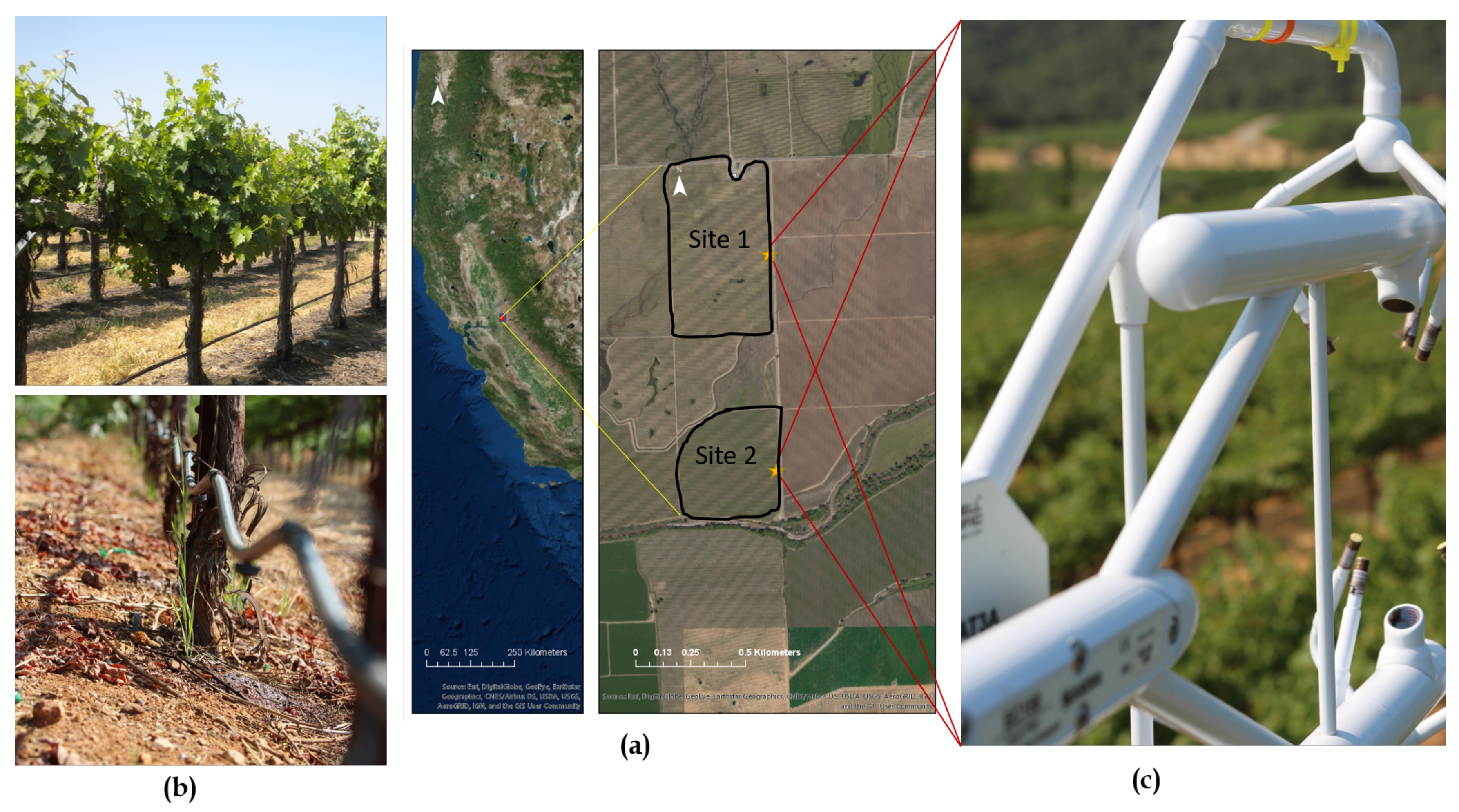
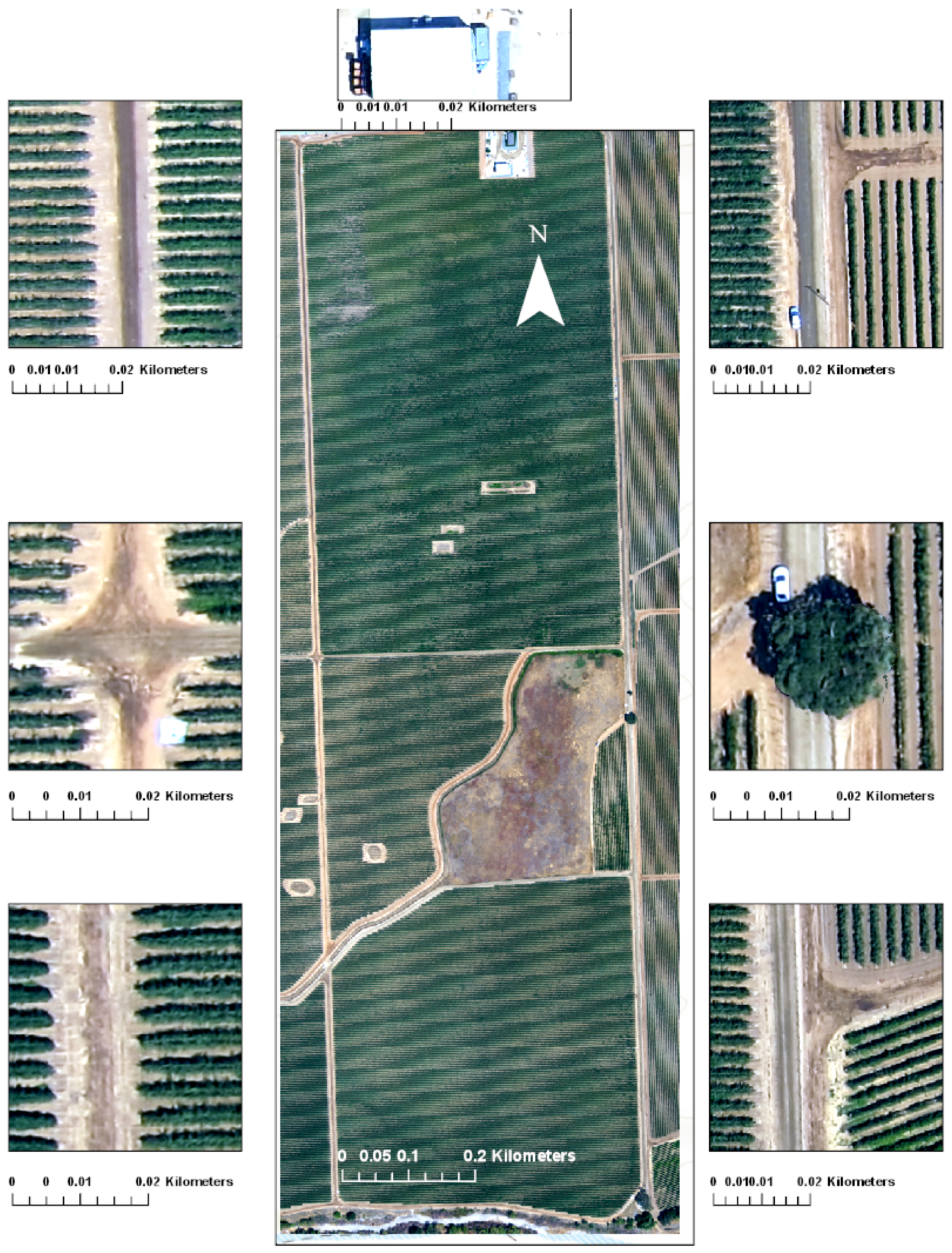
2.1. Site Description
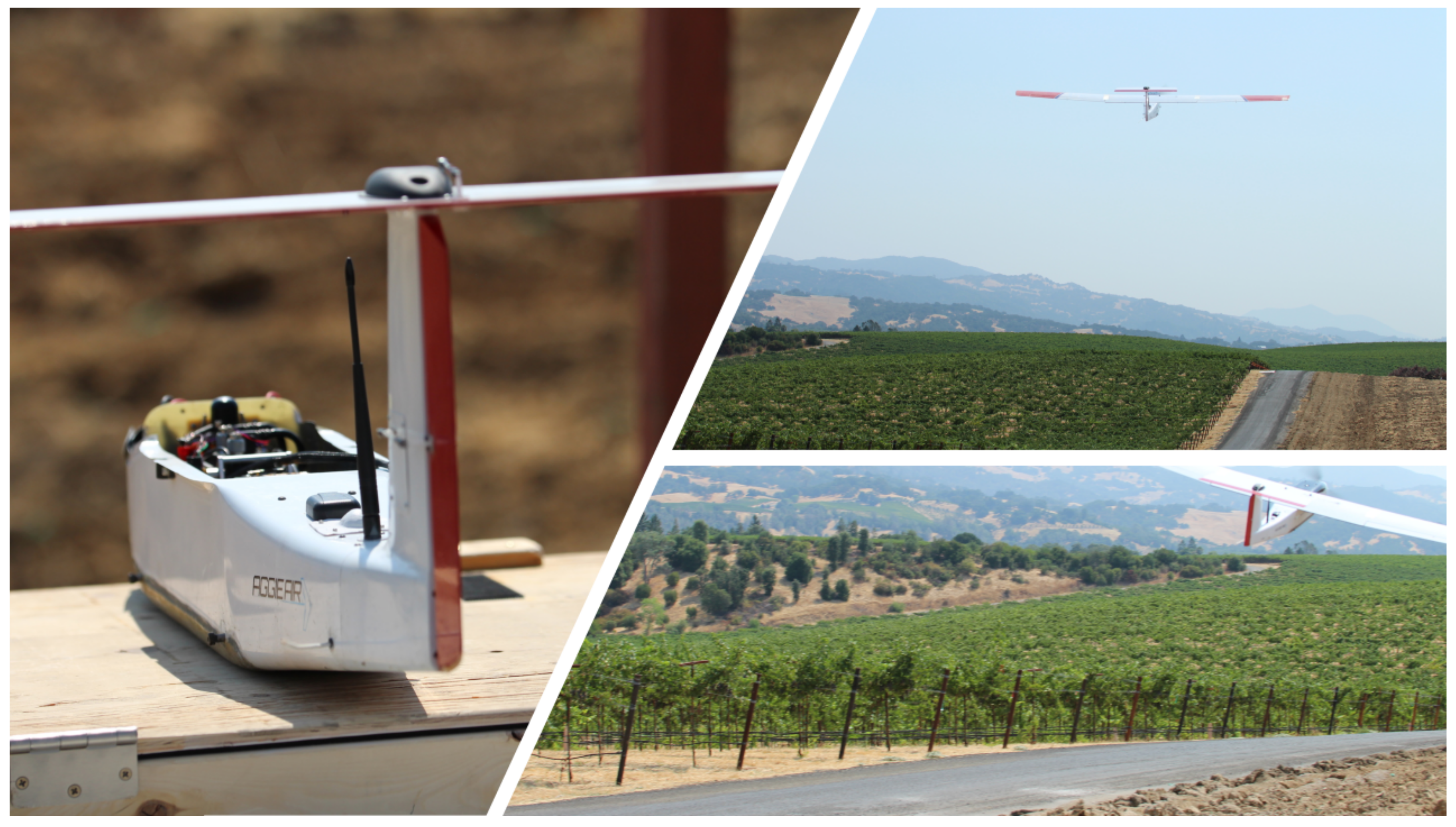
2.2. AggieAir Remote Sensing Platform
2.3. AggieAir UAV High-Resolution Imagery
2.4. AggieAir UAV Image Processing
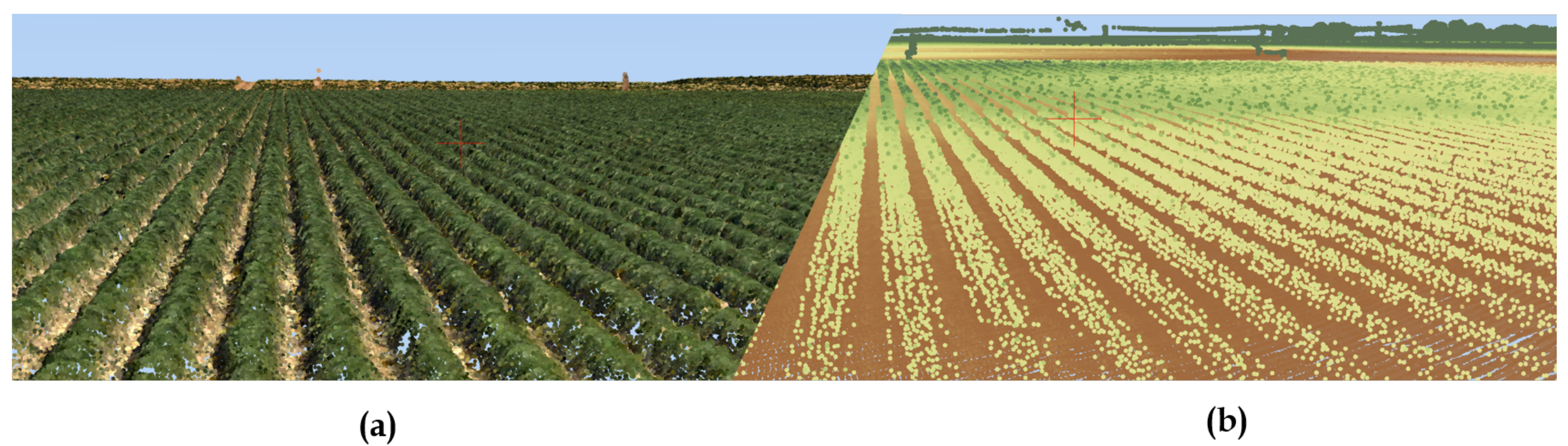
2.5. Field Measurements, Multi-Spectral Imagery, Point Cloud, and LiDAR Datasets
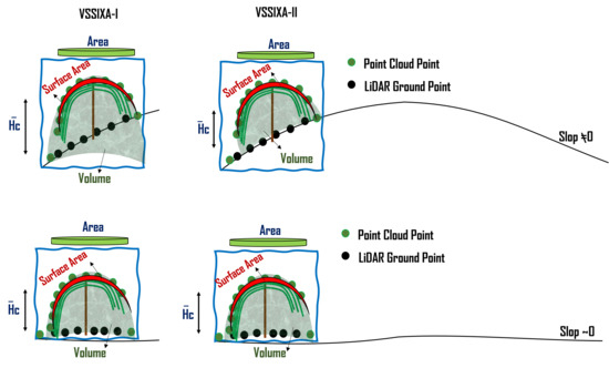
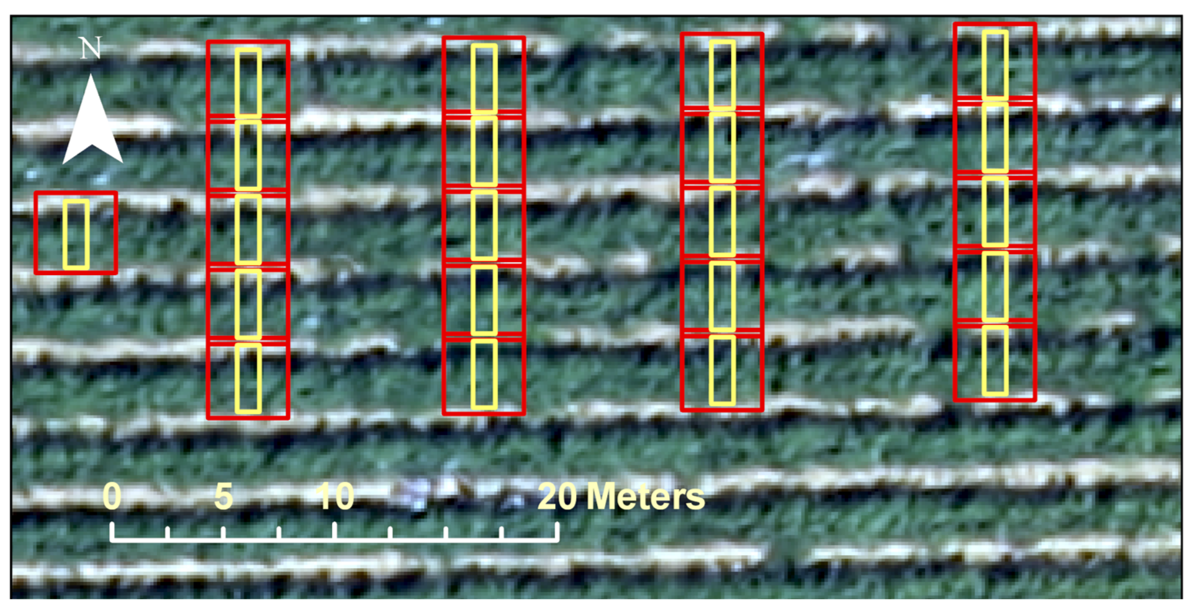
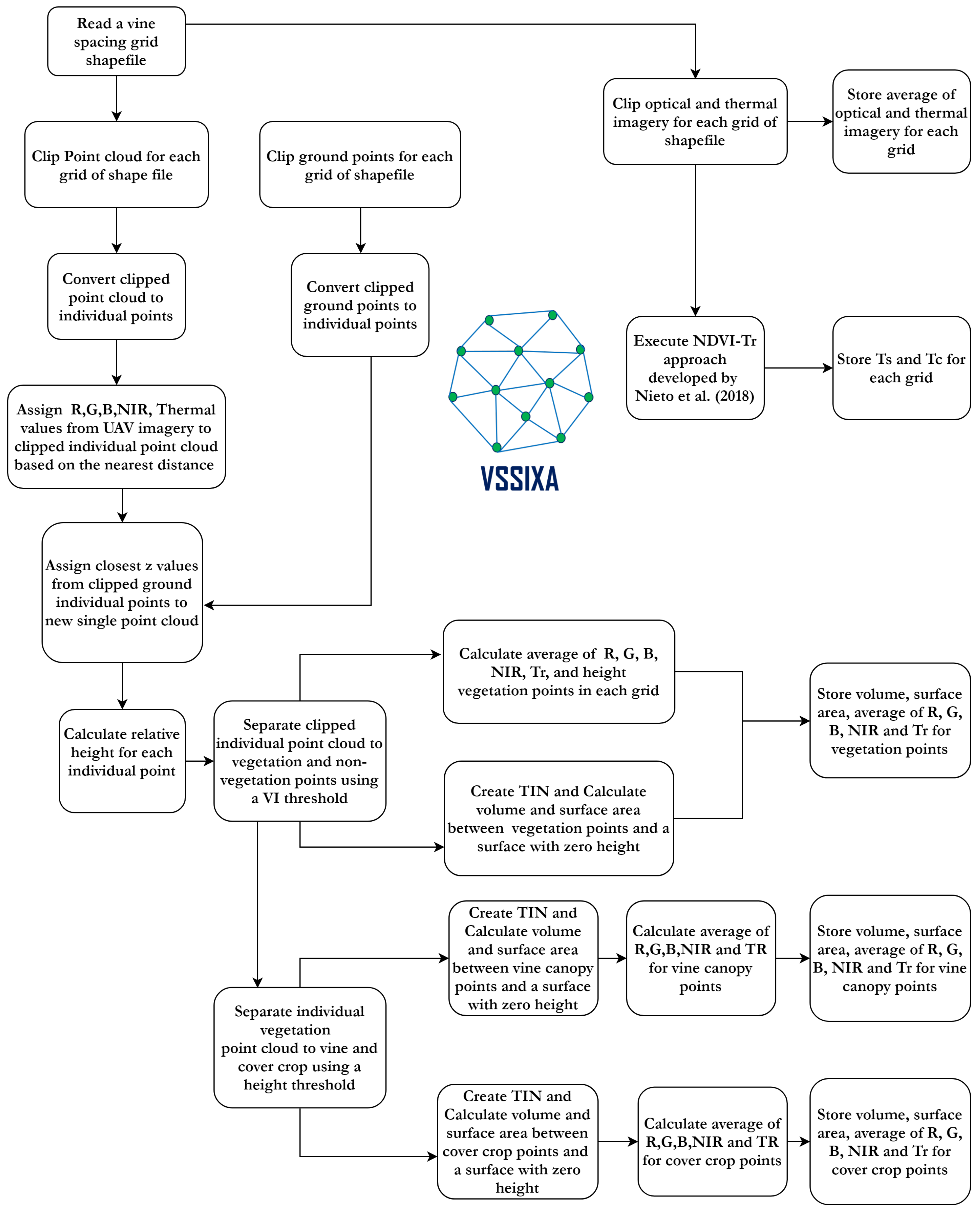
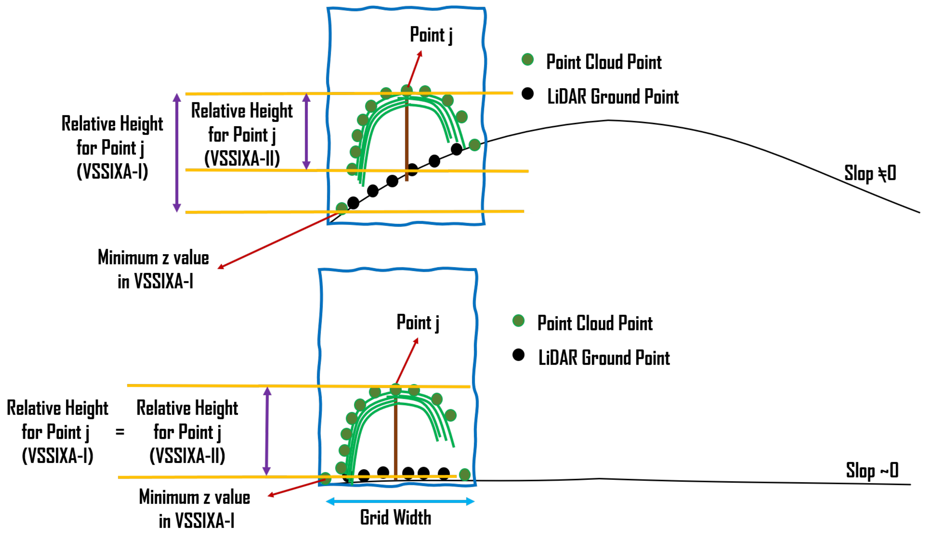
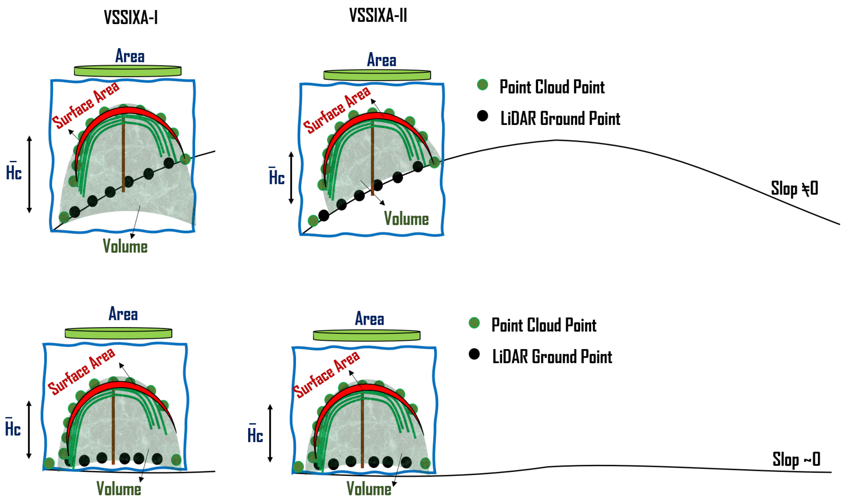
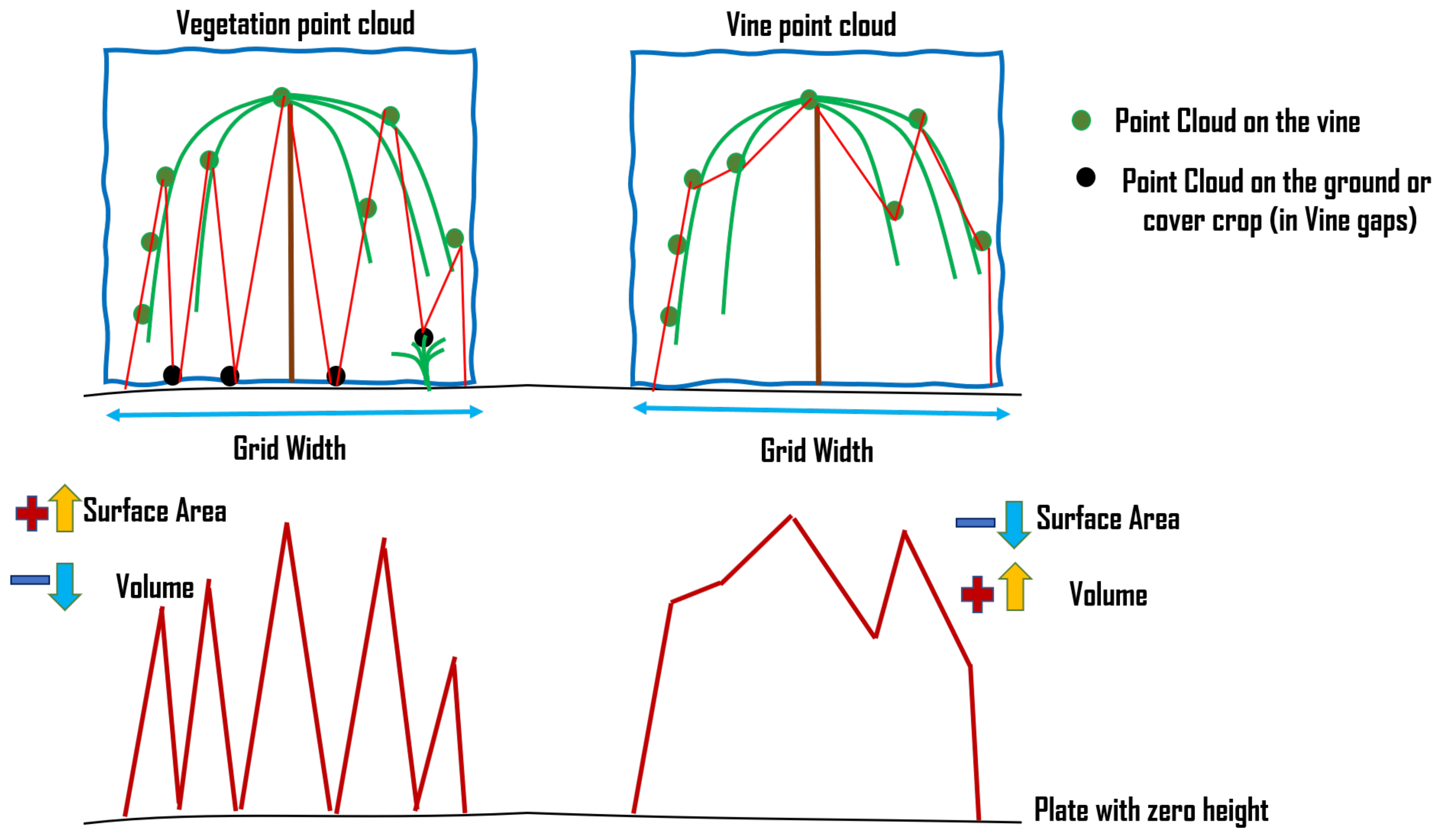
2.6. Vegetation Structural-Spectral Information Extraction Algorithm (VSSIXA)
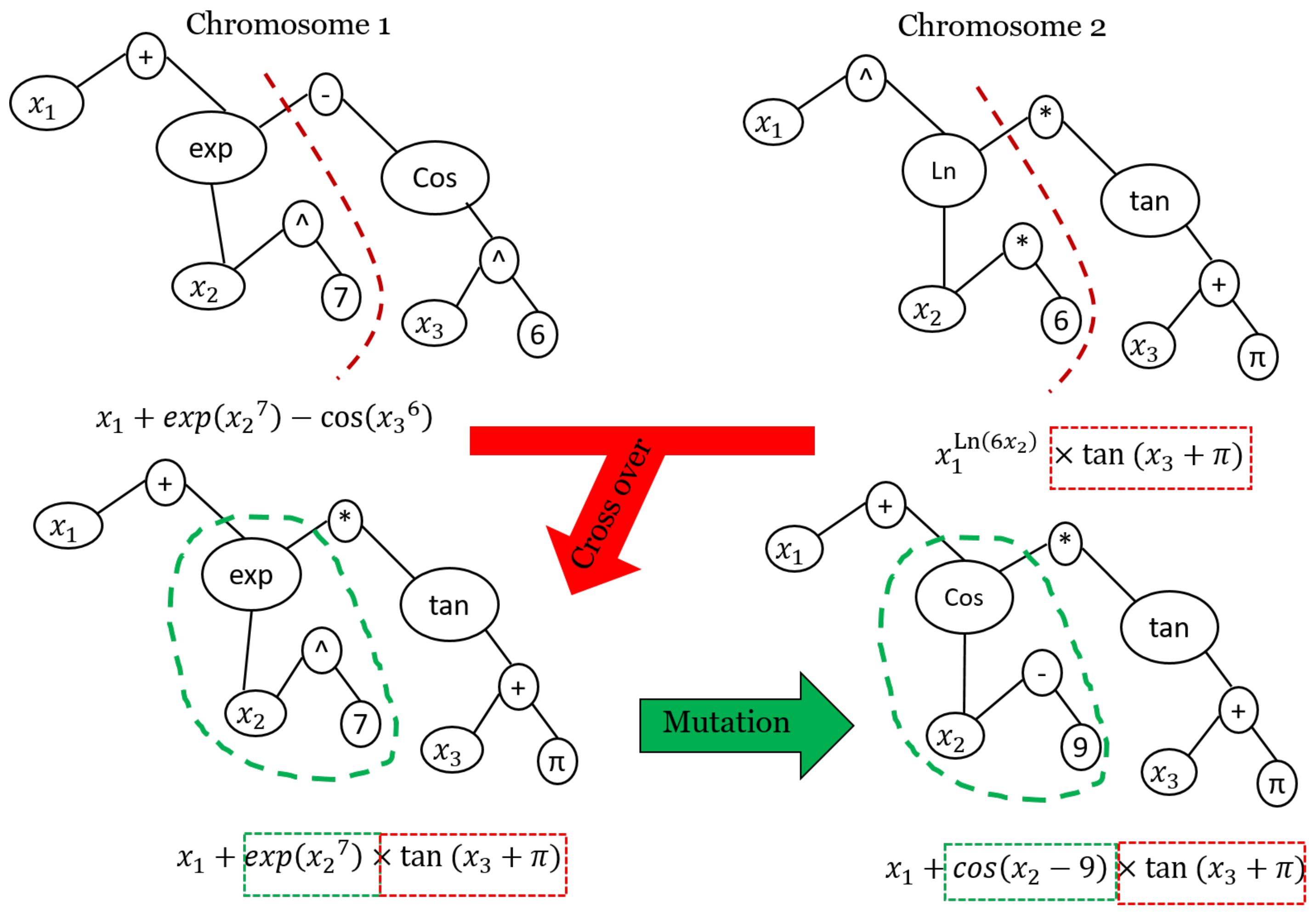
Genetic Programming: GP
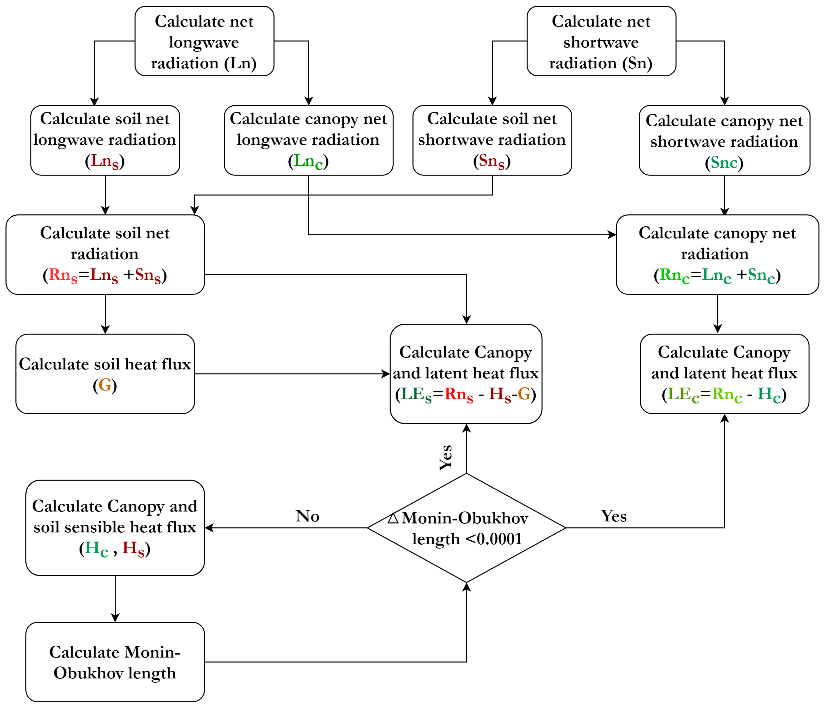
2.7. TSEB-2T Model
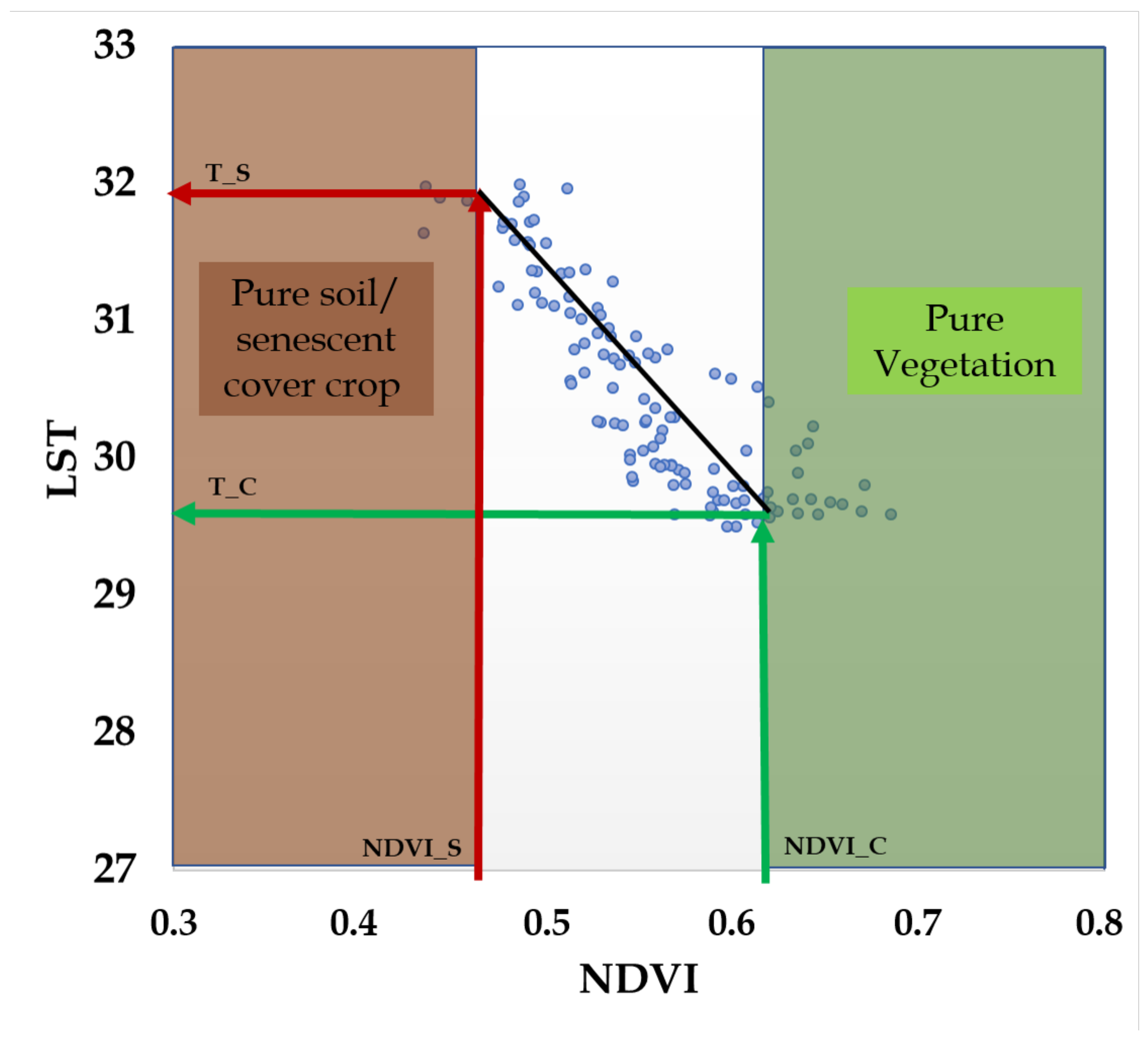
2.8. Data Analysis
3. Results
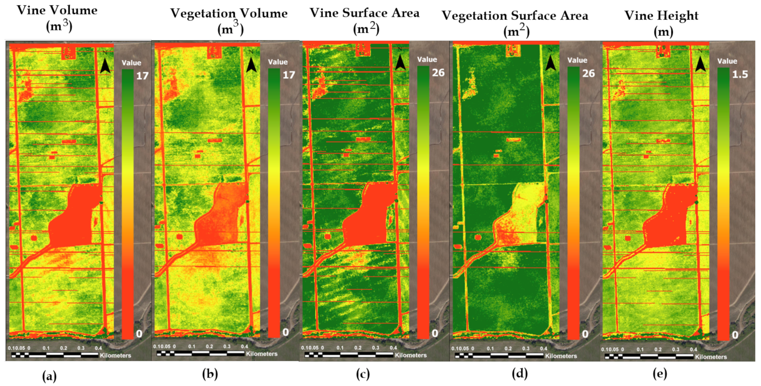
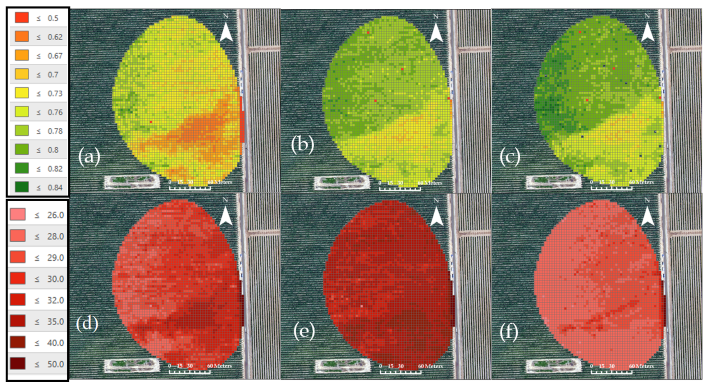
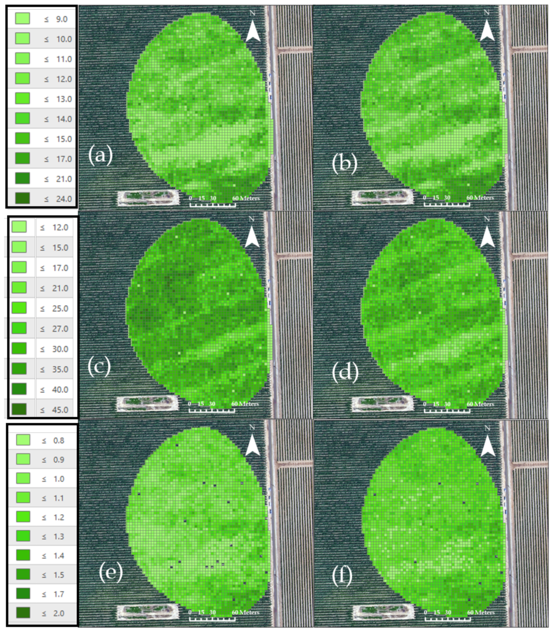
3.1. VSSIXA Outputs
3.2. Computation Time of VSSIXA
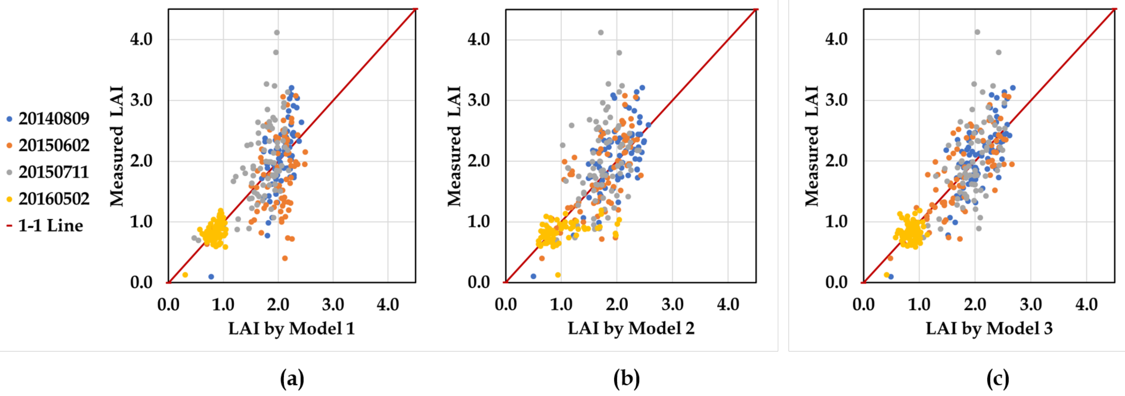
3.3. In-Situ LAI versus VSSIXA Outputs
3.4. Modeled LAI with Machine Learning Algorithms
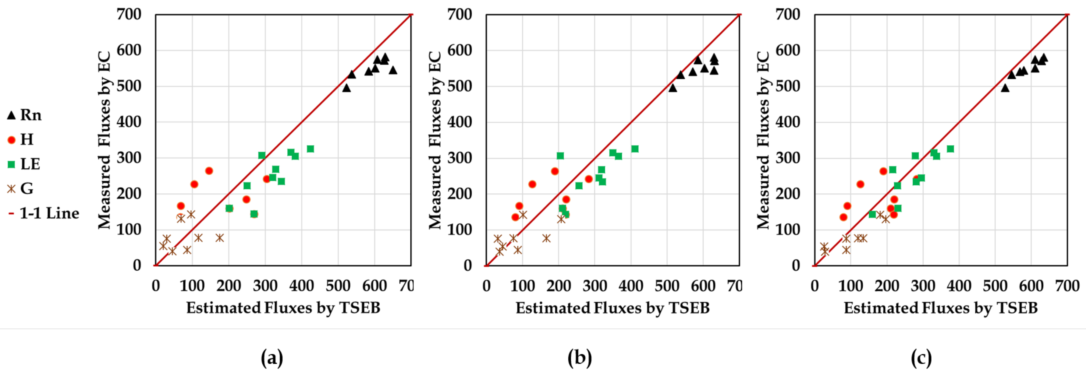
3.5. TSEB-2T Model versus Eddy Covariance Measurements
4. Discussion
5. Conclusions
Author Contributions
Funding
Acknowledgments
Conflicts of Interest
Abbreviations
| UAV | Unmanned Aerial Vehicles |
| TSEB | Two-Source Energy Balance Model |
| VSSIXA | Vegetation Structural-Spectral Information eXtraction Algorithm |
| LAI | Leaf Area Index |
| GRAPEX | Grape Remote sensing Atmospheric Profile and Evapotranspiration eXperiment |
| VIs | Vegetation indices |
| R | Red |
| G | Green |
| B | Blue |
| NIR | Near-Infrared |
| NDVI | Normalized Difference Vegetation Index |
| DSM | Digital Surface Models |
| SfM | Structure from Motion |
| MVS | Multiview-Stereo |
| LiDAR | Light Detection and Ranging |
| CSM | Crop Surface Model |
| GCP | Ground Control Points |
| CHM | Canopy Height Model |
| DEM | Digital Elevation Model |
| DTM | Digital Terrain Model |
| Radiometric Temperature | |
| USU | Utah State University |
| IMU | Inertial Measurement Unit |
| VNIR | Visible and Near-Infrared |
| Soil Temperature | |
| Canopy Temperature | |
| TIN | Triangulated Irregular Network |
| CSV | Comma-Separated Value |
| ANN | Artificial Neural Network |
| SVM | Support Vector Machine |
| GP | Genetic Programming |
| IOP | Intensive Observation Period |
| ASTER | Advanced Spaceborne Thermal Emission and Reflection Radiometer |
| agl | above ground level |
| ESRI | Environmental Systems Research Institute |
| USU | Utah State University |
| G-LiHT | Goddard’s LiDAR, Hyperspectral & Thermal Imager |
| IRGA | Infrared Gas Analyzer |
| GA | Genetic Algorithm |
| Shortwave Radiation | |
| Longwave Radiation | |
| Canopy Net Longwave Radiation | |
| Soil Net Longwave Radiation | |
| Canopy Net Shortwave Radiation | |
| Soil Net Shortwave Radiation | |
| Canopy Net Radiation | |
| Soil Net Radiation | |
| G | Soil Heat Flux |
| Sensible Heat Flux for Canopy | |
| Sensible Heat Flux for Soil | |
| Latent Heat Flux for Canopy | |
| Latent Heat Flux for Soil | |
| Coefficient of Determination | |
| MAE | Mean Absolute Error |
| RMSE | Root Mean Square Error |
| RRMSE | Relative Root Mean Square Error |
| RTK | Real-Time Kinematic |
| Average of R for Vegetation | |
| Average of G for Vegetation | |
| Average of B for Vegetation | |
| Average of N for Vegetation | |
| Average of NDVI for Vegetation | |
| Average of Vegetation Heights | |
| Volume of Vegetation | |
| Surface area of Vegetation | |
| Projected of | |
| Average of R for Vine Canopy | |
| Average of G for Vine Canopy | |
| Average of B for Vine Canopy | |
| Average of N for Vine Canopy | |
| Average of NDVI for Vine Canopy | |
| Average of Vine Canopy Height | |
| Volume of Vine Canopy | |
| Surface Area of Vine Canopy | |
| Projected of | |
| Fractional Cover | |
| Canopy Width | |
| Scenario 1 | |
| Scenario 2 | |
| Scenario 3 |
Appendix A


References
- Colaizzi, P.D.; Kustas, W.P.; Anderson, M.C.; Agam, N.; Tolk, J.A.; Evett, S.R.; Howell, T.A.; Gowda, P.H.; O’Shaughnessy, S.A. Two-source energy balance model estimates of evapotranspiration using component and composite surface temperatures. Adv. Water Resour. 2012, 50, 134–151. [Google Scholar] [CrossRef] [Green Version]
- Tang, R.; Li, Z.L.; Jia, Y.; Li, C.; Sun, X.; Kustas, W.P.; Anderson, M.C. An intercomparison of three remote sensing-based energy balance models using Large Aperture Scintillometer measurements over a wheat–corn production region. Remote Sens. Environ. 2011, 115, 3187–3202. [Google Scholar] [CrossRef]
- Timmermans, W.J.; Kustas, W.P.; Anderson, M.C.; French, A.N. An intercomparison of the Surface Energy Balance Algorithm for Land (SEBAL) and the Two-Source Energy Balance (TSEB) modeling schemes. Remote Sens. Environ. 2007, 108, 369–384. [Google Scholar] [CrossRef]
- Anderson, M.C.; Norman, J.M.; Kustas, W.P.; Li, F.; Prueger, J.H.; Mecikalski, J.R. Effects of Vegetation Clumping on Two–Source Model Estimates of Surface Energy Fluxes from an Agricultural Landscape during SMACEX. J. Hydrometeorol. 2005, 6, 892–909. [Google Scholar] [CrossRef]
- Norman, J.; Kustas, W.; Humes, K. Source approach for estimating soil and vegetation energy fluxes in observations of directional radiometric surface temperature. Agric. For. Meteorol. 1995, 77, 263–293. [Google Scholar] [CrossRef]
- Aboutalebi, M.; Torres-Rua, A.F.; Allen, N. Multispectral remote sensing for yield estimation using high-resolution imagery from an unmanned aerial vehicle. In Proceedings of the Autonomous Air and Ground Sensing Systems for Agricultural Optimization and Phenotyping III, Orlando, FL, USA, 15–19 April 2018; Volume 10664. [Google Scholar] [CrossRef]
- Kumar, L.; Schmidt, K.; Dury, S.; Skidmore, A. Imaging Spectrometry and Vegetation Science. In Imaging Spectrometry: Basic Principles and Prospective Applications; Meer, F.D.v.d., Jong, S.M.D., Eds.; Springer: Dordrecht, The Netherlands, 2001; pp. 111–155. [Google Scholar] [CrossRef]
- Xue, J.; Su, B. Significant Remote Sensing Vegetation Indices: A Review of Developments and Applications. J. Sensors 2017, 2017. [Google Scholar] [CrossRef] [Green Version]
- Sun, L.; Gao, F.; Anderson, M.C.; Kustas, W.P.; Alsina, M.M.; Sanchez, L.; Sams, B.; McKee, L.; Dulaney, W.; White, W.A.; et al. Daily Mapping of 30 m LAI and NDVI for Grape Yield Prediction in California Vineyards. Remote Sens. 2017, 9, 317. [Google Scholar] [CrossRef] [Green Version]
- Asrar, G.; Fuchs, M.; Kanemasu, E.T.; Hatfield, J.L. Estimating Absorbed Photosynthetic Radiation and Leaf Area Index from Spectral Reflectance in Wheat. Agron. J. 1989, 76, 300–306. [Google Scholar] [CrossRef]
- Serrano, L.; Filella, I.; Peñuelas, J. Remote sensing of biomass and yield of winter wheat under different nitrogen supplies. Crop. Sci. 2000, 40, 723–731. [Google Scholar] [CrossRef] [Green Version]
- Bendig, J.; Yu, K.; Aasen, H.; Bolten, A.; Bennertz, S.; Broscheit, J.; Gnyp, M.L.; Bareth, G. Combining UAV-based plant height from crop surface models, visible, and near infrared vegetation indices for biomass monitoring in barley. Int. J. Appl. Earth Obs. Geoinf. 2015, 39, 79–87. [Google Scholar] [CrossRef]
- Diarra, A.; Jarlan, L.; Er-Raki, S.; Page, M.L.; Aouade, G.; Tavernier, A.; Boulet, G.; Ezzahar, J.; Merlin, O.; Khabba, S. Performance of the two-source energy budget (TSEB) model for the monitoring of evapotranspiration over irrigated annual crops in North Africa. Agric. Water Manag. 2017, 193, 71–88. [Google Scholar] [CrossRef]
- White, W.A.; Alsina, M.M.; Nieto, H.; McKee, L.G.; Gao, F.; Kustas, W.P. Determining a robust indirect measurement of leaf area index in California vineyards for validating remote sensing-based retrievals. Irrig. Sci. 2018, 37, 269–280. [Google Scholar] [CrossRef]
- Zarco-Tejada, P.; Diaz-Varela, R.; Angileri, V.; Loudjani, P. Tree height quantification using very high resolution imagery acquired from an unmanned aerial vehicle (UAV) and automatic 3D photo-reconstruction methods. Eur. J. Agron. 2014, 55, 89–99. [Google Scholar] [CrossRef]
- Du, M.; Noguchi, N. Monitoring of Wheat Growth Status and Mapping of Wheat Yield’s within-Field Spatial Variations Using Color Images Acquired from UAV-camera System. Remote Sens. 2017, 9, 289. [Google Scholar] [CrossRef] [Green Version]
- Zermas, D.; Teng, D.; Stanitsas, P.; Bazakos, M.; Kaiser, D.; Morellas, V.; Mulla, D.; Papanikolopoulos, N. Automation solutions for the evaluation of plant health in corn fields. In Proceedings of the 2015 IEEE/RSJ International Conference on Intelligent Robots and Systems (IROS), Hamburg, Germany, 28 September–2 October 2015; pp. 6521–6527. [Google Scholar] [CrossRef]
- Santesteban, L.; Gennaro, S.D.; Herrero-Langreo, A.; Miranda, C.; Royo, J.; Matese, A. High-resolution UAV-based thermal imaging to estimate the instantaneous and seasonal variability of plant water status within a vineyard. Agric. Water Manag. 2017, 183, 49–59. [Google Scholar] [CrossRef]
- Jiménez-Bello, M.A.; Royuela, A.; Manzano, J.; Zarco-Tejada, P.J.; Intrigliolo, D. Assessment of drip irrigation sub-units using airborne thermal imagery acquired with an Unmanned Aerial Vehicle (UAV). In Precision Agriculture ’13; Stafford, J.V., Ed.; Wageningen Academic Publishers: Wageningen, The Netherlands, 2013; pp. 705–711. [Google Scholar]
- Holman, F.H.; Riche, A.B.; Michalski, A.; Castle, M.; Wooster, M.J.; Hawkesford, M.J. High Throughput Field Phenotyping of Wheat Plant Height and Growth Rate in Field Plot Trials Using UAV Based Remote Sensing. Remote Sens. 2016, 8, 1031. [Google Scholar] [CrossRef]
- Vanegas, F.; Bratanov, D.; Powell, K.; Weiss, J.; Gonzalez, F. A Novel Methodology for Improving Plant Pest Surveillance in Vineyards and Crops Using UAV-Based Hyperspectral and Spatial Data. Sensors 2018, 18, 260. [Google Scholar] [CrossRef] [Green Version]
- Rasmussen, J.; Nielsen, J.; Garcia-Ruiz, F.; Christensen, S.; Streibig, J.C. Potential uses of small unmanned aircraft systems (UAS) in weed research. Weed Res. 2013, 53, 242–248. [Google Scholar] [CrossRef]
- Rokhmana, C.A. The Potential of UAV-based Remote Sensing for Supporting Precision Agriculture in Indonesia. Procedia Environ. Sci. 2015, 24, 245–253. [Google Scholar] [CrossRef] [Green Version]
- Comba, L.; Biglia, A.; Aimonino, D.R.; Gay, P. Unsupervised detection of vineyards by 3D point-cloud UAV photogrammetry for precision agriculture. Comput. Electron. Agric. 2018, 155, 84–95. [Google Scholar] [CrossRef]
- Fraser, R.H.; Olthof, I.; Lantz, T.C.; Schmitt, C. UAV photogrammetry for mapping vegetation in the low-Arctic. Arct. Sci. 2016, 2, 79–102. [Google Scholar] [CrossRef] [Green Version]
- Thiel, C.; Schmullius, C. Comparison of UAV photograph-based and airborne lidar-based point clouds over forest from a forestry application perspective. Int. J. Remote Sens. 2017, 38, 2411–2426. [Google Scholar] [CrossRef]
- Yilmaz, V.; Konakoglu, B.; Serifoglu, C.; Gungor, O.; Gökalp, E. Image classification-based ground filtering of point clouds extracted from UAV-based aerial photos. Geocarto Int. 2018, 33, 310–320. [Google Scholar] [CrossRef]
- Hu, X.; Zhang, Z.; Duan, Y.; Zhang, Y.; Zhu, J.; Long, H. Lidar Photogrammetry and Its Data Organization. ISPRS-Int. Arch. Photogramm. Remote Sens. Spat. Inf. Sci. 2011, XXXVIII-5/W12, 181–184. [Google Scholar]
- Küng, O.; Strecha, C.; Beyeler, A.; Zufferey, J.C.; Floreano, D.; Fua, P.; Gervaix, F. The accuracy of automatic photogrammetric techniques on ultra-light UAV imagery. Int. Arch. Photogramm. Remote Sens. Spat. Inf. Sci.-ISPRS Arch. 2011, 38, 125–130. [Google Scholar] [CrossRef] [Green Version]
- Rock, G.; Ries, J.B.; Udelhoven, T. Sensitivity Analysis of Uav-Photogrammetry for Creating Digital Elevation Models (DEM). ISPRS-Int. Arch. Photogramm. Remote Sens. Spat. Inf. Sci. 2011, XXXVIII-1/C22, 69–73. [Google Scholar] [CrossRef] [Green Version]
- Amrullah, C.; Suwardhi, D.; Meilano, I. Product Accuracy Effect of Oblique and Vertical Non-Metric Digital Camera Utilization in Uav-Photogrammetry to Determine Fault Plane. ISPRS Ann. Photogramm. Remote Sens. Spat. Inf. Sci. 2016, III-6, 41–48. [Google Scholar] [CrossRef]
- Mesas-Carrascosa, F.J.; Notario García, M.D.; Meroño de Larriva, J.E.; García-Ferrer, A. An Analysis of the Influence of Flight Parameters in the Generation of Unmanned Aerial Vehicle (UAV) Orthomosaicks to Survey Archaeological Areas. Sensors 2016, 16, 1838. [Google Scholar] [CrossRef] [Green Version]
- Dandois, J.P.; Olano, M.; Ellis, E.C. Optimal Altitude, Overlap, and Weather Conditions for Computer Vision UAV Estimates of Forest Structure. Remote Sens. 2015, 7, 13895–13920. [Google Scholar] [CrossRef] [Green Version]
- Verhoeven, G. Taking computer vision aloft—Archaeological three-dimensional reconstructions from aerial photographs with photoscan. Archaeol. Prospect. 2011, 18, 67–73. [Google Scholar] [CrossRef]
- Tahar, K.N.; Ahmad, A. An Evaluation on Fixed Wing and Multi-Rotor UAV Images Using Photogrammetric Image Processing. Int. J. Comput. Electr. Autom. Control. Inf. Eng. 2013, 7, 48–52. [Google Scholar]
- Jaud, M.; Passot, S.; Le Bivic, R.; Delacourt, C.; Grandjean, P.; Le Dantec, N. Assessing the Accuracy of High Resolution Digital Surface Models Computed by PhotoScan® and MicMac® in Sub-Optimal Survey Conditions. Remote Sens. 2016, 8, 465. [Google Scholar] [CrossRef] [Green Version]
- Martínez-Carricondo, P.; Agüera-Vega, F.; Carvajal-Ramírez, F.; Mesas-Carrascosa, F.J.; García-Ferrer, A.; Pérez-Porras, F.J. Assessment of UAV-photogrammetric mapping accuracy based on variation of ground control points. Int. J. Appl. Earth Obs. Geoinf. 2018, 72, 1–10. [Google Scholar] [CrossRef]
- Aboutalebi, M.; Torres-Rua, A.F.; McKee, M.; Kustas, W.; Nieto, H.; Coopmans, C. Validation of digital surface models (DSMs) retrieved from unmanned aerial vehicle (UAV) point clouds using geometrical information from shadows. In Proceedings of the Autonomous Air and Ground Sensing Systems for Agricultural Optimization and Phenotyping IV, Baltimore, MD, USA, 14–18 April 2019; Volume 11008. [Google Scholar] [CrossRef]
- Aboutalebi, M.; Torres-Rua, A.F.; Kustas, W.P.; Nieto, H.; Coopmans, C.; McKee, M. Assessment of different methods for shadow detection in high-resolution optical imagery and evaluation of shadow impact on calculation of NDVI, and evapotranspiration. Irrig. Sci. 2019, 37, 407–429. [Google Scholar] [CrossRef]
- Garousi-Nejad, I.; Tarboton, D.; Aboutalebi, M.; Torres-Rua, A. Terrain Analysis Enhancements to the Height Above Nearest Drainage Flood Inundation Mapping Method. Water Resour. Res. 2019, 55, 7983–8009. [Google Scholar] [CrossRef]
- Jensen, J.L.R.; Mathews, A.J. Assessment of Image-Based Point Cloud Products to Generate a Bare Earth Surface and Estimate Canopy Heights in a Woodland Ecosystem. Remote Sens. 2016, 8, 50. [Google Scholar] [CrossRef] [Green Version]
- Panagiotidis, D.; Abdollahnejad, A.; Surový, P.; Chiteculo, V. Determining Tree Height and Crown Diameter from High-resolution UAV Imagery. Int. J. Remote Sens. 2017, 38, 2392–2410. [Google Scholar] [CrossRef]
- Díaz-Varela, R.A.; De la Rosa, R.; León, L.; Zarco-Tejada, P.J. High-Resolution Airborne UAV Imagery to Assess Olive Tree Crown Parameters Using 3D Photo Reconstruction: Application in Breeding Trials. Remote Sens. 2015, 7, 4213–4232. [Google Scholar] [CrossRef] [Green Version]
- Karpina, M.; Jarząbek-Rychard, M.; Tymków, P.; Borkowski, A. Uav-Based Automatic Tree Growth Measurement for Biomass Estimation. ISPRS-Int. Arch. Photogramm. Remote Sens. Spat. Inf. Sci. 2016, XLI-B8, 685–688. [Google Scholar] [CrossRef]
- Kattenborn, T.; Sperlich, M.; Bataua, K.; Koch, B. Automatic Single Tree Detection in Plantations using UAV-based Photogrammetric Point clouds. ISPRS-Int. Arch. Photogramm. Remote Sens. Spat. Inf. Sci. 2014, XL-3, 139–144. [Google Scholar] [CrossRef] [Green Version]
- Bendig, J.; Willkomm, M.; Tilly, N.; Gnyp, M.L.; Bennertz, S.; Qiang, C.; Miao, Y.; Lenz-Wiedemann, V.I.S.; Bareth, G. Very high resolution crop surface models (CSMs) from UAV-based stereo images for rice growth monitoring In Northeast China. ISPRS-Int. Arch. Photogramm. Remote Sens. Spat. Inf. Sci. 2013, XL-1/W2, 45–50. [Google Scholar] [CrossRef] [Green Version]
- Bendig, J.; Bolten, A.; Bennertz, S.; Broscheit, J.; Eichfuss, S.; Bareth, G. Estimating Biomass of Barley Using Crop Surface Models (CSMs) Derived from UAV-Based RGB Imaging. Remote Sens. 2014, 6, 10395–10412. [Google Scholar] [CrossRef] [Green Version]
- Gitelson, A.A.; Viña, A.; Arkebauer, T.J.; Rundquist, D.C.; Keydan, G.; Leavitt, B. Remote estimation of leaf area index and green leaf biomass in maize canopies. Geophys. Res. Lett. 2003, 30. [Google Scholar] [CrossRef] [Green Version]
- Honkavaara, E.; Kaivosoja, J.; Mäkynen, J.; Pellikka, I.; Pesonen, L.; Saari, H.; Salo, H.; Hakala, T.; Marklelin, L.; Rosnell, T. Hyperspectral Reflectance Signatures and Point Clouds for Precision Agriculture by Light Weight Uav Imaging System. ISPRS Ann. Photogramm. Remote Sens. Spat. Inf. Sci. 2012, I-7, 353–358. [Google Scholar] [CrossRef] [Green Version]
- Duan, T.; Zheng, B.; Guo, W.; Ninomiya, S.; Guo, Y.; Chapman, S.C. Comparison of ground cover estimates from experiment plots in cotton, sorghum and sugarcane based on images and ortho-mosaics captured by UAV. Funct. Plant Biol. 2017, 44, 169–183. [Google Scholar] [CrossRef]
- Calera, A.; Martínez, C.; Melia, J. A procedure for obtaining green plant cover: Relation to NDVI in a case study for barley. Int. J. Remote Sens. 2001, 22, 3357–3362. [Google Scholar] [CrossRef]
- Matese, A.; Gennaro, S.F.D.; Berton, A. Assessment of a canopy height model (CHM) in a vineyard using UAV-based multispectral imaging. Int. J. Remote Sens. 2017, 38, 2150–2160. [Google Scholar] [CrossRef]
- Mathews, A.J.; Jensen, J.L.R. Visualizing and Quantifying Vineyard Canopy LAI Using an Unmanned Aerial Vehicle (UAV) Collected High Density Structure from Motion Point Cloud. Remote Sens. 2013, 5, 2164–2183. [Google Scholar] [CrossRef] [Green Version]
- Weiss, M.; Baret, F. Using 3D Point Clouds Derived from UAV RGB Imagery to Describe Vineyard 3D Macro-Structure. Remote Sens. 2017, 9, 111. [Google Scholar] [CrossRef] [Green Version]
- Kustas, W.P.; Anderson, M.C.; Alfieri, J.G.; Knipper, K.; Torres-Rua, A.; Parry, C.K.; Nieto, H.; Agam, N.; White, A.; Gao, F.; et al. The Grape Remote Sensing Atmospheric Profile and Evapotranspiration Experiment (GRAPEX). Bull. Amer. Meteorol. Soc. 2018, 99, 1791–1812. [Google Scholar] [CrossRef] [Green Version]
- Elarab, M.; Ticlavilca, A.M.; Torres-Rua, A.F.; Maslova, I.; McKee, M. Estimating chlorophyll with thermal and broadband multispectral high resolution imagery from an unmanned aerial system using relevance vector machines for precision agriculture. Int. J. Appl. Earth Obs. Geoinf. 2015, 43, 32–42. [Google Scholar] [CrossRef] [Green Version]
- Hassan-Esfahani, L.; Torres-Rua, A.; Jensen, A.; McKee, M. Assessment of Surface Soil Moisture Using High-Resolution Multi-Spectral Imagery and Artificial Neural Networks. Remote Sens. 2015, 7, 2627–2646. [Google Scholar] [CrossRef] [Green Version]
- Aggieair. Available online: https://uwrl.usu.edu/aggieair/ (accessed on 15 December 2019).
- Labsphere. Available online: https://www.labsphere.com (accessed on 15 December 2019).
- Neale, C.M.; Crowther, B.G. An airborne multispectral video/radiometer remote sensing system: Development and calibration. Remote Sens. Environ. 1994, 49, 187–194. [Google Scholar] [CrossRef]
- Miura, T.; Huete, A. Performance of three reflectance calibration methods for airborne hyperspectral spectrometer data. Sensors 2009, 9, 794–813. [Google Scholar] [CrossRef] [Green Version]
- Crowther, B. Radiometric Calibration of Multispectral Video Imagery. Ph.D. Thesis, Utah State University, Logan, UT, USA, 1992. [Google Scholar]
- Agisoft, L.L.; St Petersburg, R. Agisoft Photoscan; Professional ed.; 2014. [Google Scholar]
- Aboutalebi, M.; Torres-Rua, A.F.; McKee, M.; Nieto, H.; Kustas, W.P.; Prueger, J.H.; McKee, L.; Alfieri, J.G.; Hipps, L.; Coopmans, C. Assessment of Landsat Harmonized sUAS Reflectance Products Using Point Spread Function (PSF) on Vegetation Indices (VIs) and Evapotranspiration (ET) Using the Two-Source Energy Balance (TSEB) Model. AGU Fall Meet. Abstr. 2018. Available online: https://ui.adsabs.harvard.edu/abs/2018AGUFM.H33I2193A/abstract (accessed on 15 December 2019).
- Torres-Rua, A. Vicarious Calibration of sUAS Microbolometer Temperature Imagery for Estimation of Radiometric Land Surface Temperature. Sensors 2017, 17, 1499. [Google Scholar] [CrossRef] [Green Version]
- Cook, B.; Corp, L.W.; Nelson, R.F.; Middleton, E.M.; Morton, D.C.; McCorkel, J.T.; Masek, J.G.; Ranson, K.J.; Ly, V.; Montesano, P.M. NASA Goddard’s Lidar, Hyperspectral and Thermal (G-LiHT) airborne imager. Remote Sens. 2013, 5, 4045–4066. [Google Scholar] [CrossRef] [Green Version]
- Nieto, H.; Kustas, W.P.; Torres-Rúa, A.; Alfieri, J.G.; Gao, F.; Anderson, M.C.; White, W.A.; Song, L.; Alsina, M.d.M.; Prueger, J.H.; et al. Evaluation of TSEB turbulent fluxes using different methods for the retrieval of soil and canopy component temperatures from UAV thermal and multispectral imagery. Irrig. Sci. 2019, 37, 389–406. [Google Scholar] [CrossRef] [Green Version]
- Schotanus, P.; Nieuwstadt, F.; De Bruin, H. Temperature measurement with a sonic anemometer and its application to heat and moisture fluxes. Bound.-Layer Meteorol. 1983, 26, 81–93. [Google Scholar] [CrossRef]
- Liu, H.; Peters, G.; Foken, T. New equations for sonic temperature variance And buoyancy heat flux with an omnidirectional sonic anemometer. Bound.-Layer Meteorol. 2001, 100, 459–468. [Google Scholar] [CrossRef]
- Tanner, C.B.; Thurtell, G.W.T. Anemoclinometer Measurements of Reynolds Stress and Heat Transport in the Atmospheric Surface Layer; Research and Development Technical Report ECOM 66-G22-F to the US Army Electronics Command; Dept. of Soil Science, Univ. of Wisconsin: Madison, WI, USA, 1969. [Google Scholar]
- Massman, W. A simple method for estimating frequency response corrections for eddy covariance systems. Agric. For. Meteorol. 2000, 104, 185–198. [Google Scholar] [CrossRef]
- Webb, E.K.; Pearman, G.I.; Leuning, R. Correction of flux measurements for density effects due to heat and water vapour transfer. Q. J. R. Meteorol. Soc. 1980, 106, 85–100. [Google Scholar] [CrossRef]
- Foken, T. The Energy Balance Closure Problem: An Overview. Ecol. Appl. 2008, 18, 1351–1367. [Google Scholar] [CrossRef] [PubMed]
- Oke, T. Boundary Layer Climates, 2nd ed.; Cambridge University Press: Cambridge, UK, 1987. [Google Scholar]
- Twine, T.; Kustas, W.; Norman, J.; Cook, D.; Houser, P.; Meyers, T.; Prueger, J.; Starks, P.; Wesely, M. Correcting eddy-covariance flux underestimates over a grassland. Agric. For. Meteorol. 2000, 103, 279–300. [Google Scholar] [CrossRef] [Green Version]
- Wilson, K.; Goldstein, A.; Falge, E.; Aubinet, M.; Baldocchi, D.; Berbigier, P.; Bernhofer, C.; Ceulemans, R.; Dolman, H.; Field, C.; et al. Energy balance closure at FLUXNET sites. Agric. For. Meteorol. 2002, 113, 223–243. [Google Scholar] [CrossRef] [Green Version]
- Frank, J.M.; Massman, W.J.; Ewers, B.E. A Bayesian model to correct underestimated 3-D wind speeds from sonic anemometers increases turbulent components of the surface energy balance. Atmos. Meas. Tech. 2016, 9, 5933–5953. [Google Scholar] [CrossRef]
- Frank, J.M.; Massman, W.J.; Ewers, B.E. Underestimates of sensible heat flux due to vertical velocity measurement errors in non-orthogonal sonic anemometers. Agric. For. Meteorol. 2013, 171–172, 72–81. [Google Scholar] [CrossRef]
- Horst, T.W.; Semmer, S.R.; Maclean, G. Correction of a Non-orthogonal, Three-Component Sonic Anemometer for Flow Distortion by Transducer Shadowing. Bound.-Layer Meteorol. 2015, 155, 371–395. [Google Scholar] [CrossRef] [Green Version]
- Kochendorfer, J.; Meyers, T.P.; Frank, J.; Massman, W.J.; Heuer, M.W. How Well Can We Measure the Vertical Wind Speed? Implications for Fluxes of Energy and Mass. Bound.-Layer Meteorol. 2012, 145, 383–398. [Google Scholar] [CrossRef]
- Vegetation Spectral-Structural Information eXtraction Algorithm (VSSIXA): Working with Point cloud and LiDAR. Available online: https://github.com/Mahyarona/VSSIXA (accessed on 15 December 2019).
- Aboutalebi, M.; Allen, L.N.; Torres-Rua, A.F.; McKee, M.; Coopmans, C. Estimation of soil moisture at different soil levels using machine learning techniques and unmanned aerial vehicle (UAV) multispectral imagery. In Proceedings of the Autonomous Air and Ground Sensing Systems for Agricultural Optimization and Phenotyping IV, Baltimore, MD, USA, 14–18 April 2019; Volume 11008. [Google Scholar] [CrossRef] [Green Version]
- Schmidt, M.; Lipson, H. Distilling free-form natural laws from experimental data. Science 2009, 324, 81–85. [Google Scholar] [CrossRef]
- Schmidt, M.; Lipson, H. Eureqa (Version 0.98 beta) [Software]. 2014. Available online: www.nutonian.com (accessed on 15 December 2019).
- Kustas, W.P.; Norman, J.M. A two-source approach for estimating turbulent fluxes using multiple angle thermal infrared observations. Water Resour. Res. 1997, 33, 1495–1508. [Google Scholar] [CrossRef]
- Kustas, W.P.; Norman, J.M. Evaluation of soil and vegetation heat flux predictions using a simple two-source model with radiometric temperatures for partial canopy cover. Agric. For. Meteorol. 1999, 94, 13–29. [Google Scholar] [CrossRef]
- Campbell, G.; Norman, J. An Introduction to Environmental Biophysics; Modern Acoustics and Signal; Springer: New York, NY, USA, 2000. [Google Scholar]
- Willmott, C.J.; Matsuura, K. Advantages of the mean absolute error (MAE) over the root mean square error (RMSE) in assessing average model performance. Clim. Res. 2005, 30, 79–82. [Google Scholar] [CrossRef]
- Despotovic, M.; Nedic, V.; Despotovic, D.; Cvetanovic, S. Evaluation of empirical models for predicting monthly mean horizontal diffuse solar radiation. Renew. Sustain. Energy Rev. 2016, 56, 246–260. [Google Scholar] [CrossRef]
- Li, M.F.; Tang, X.P.; Wu, W.; Liu, H.B. General models for estimating daily global solar radiation for different solar radiation zones in mainland China. Energy Convers. Manag. 2013, 70, 139–148. [Google Scholar] [CrossRef]
- Kljun, N.; Calanca, P.; Rotach, M.W.; Schmid, H.P. A simple two-dimensional parameterisation for Flux Footprint Prediction (FFP). Geosci. Model Dev. 2015, 8, 3695–3713. [Google Scholar] [CrossRef] [Green Version]
- Agam, N.; Kustas, W.P.; Alfieri, J.G.; Gao, F.; McKee, L.M.; Prueger, J.H.; Hipps, L.E. Micro-scale spatial variability in soil heat flux (SHF) in a wine-grape vineyard. Irrig. Sci. 2019, 37, 253–268. [Google Scholar] [CrossRef]
- Gao, F.; Anderson, M.C.; Kustas, W.P.; Houborg, R. Retrieving Leaf Area Index From Landsat Using MODIS LAI Products and Field Measurements. IEEE Geosci. Remote Sens. Lett. 2014, 11, 773–777. [Google Scholar] [CrossRef]
- Gao, F.; Kustas, W.P.; Anderson, M.C. A Data Mining Approach for Sharpening Thermal Satellite Imagery over Land. Remote Sens. 2012, 4, 3287–3319. [Google Scholar] [CrossRef] [Green Version]
- Nieto, H.; Kustas, W.P.; Alfieri, J.G.; Gao, F.; Hipps, L.E.; Los, S.; Prueger, J.H.; McKee, L.G.; Anderson, M.C. Impact of different within-canopy wind attenuation formulations on modelling sensible heat flux using TSEB. Irrig. Sci. 2019, 37, 315–331. [Google Scholar] [CrossRef]
- Villagarcía, L.; Were, A.; Domingo, F.; García, M.; Alados-Arboledas, L. Estimation of soil boundary-layer resistance in sparse semiarid stands for evapotranspiration modelling. J. Hydrol. 2007, 342, 173–183. [Google Scholar] [CrossRef]
- Andreu, A.; Kustas, W.P.; Polo, M.J.; Carrara, A.; González-Dugo, M.P. Modeling Surface Energy Fluxes over a Dehesa (Oak Savanna) Ecosystem Using a Thermal Based Two-Source Energy Balance Model (TSEB) I. Remote Sens. 2018, 10, 567. [Google Scholar] [CrossRef] [Green Version]
- Chávez, J.L.; Gowda, P.H.; Howell, T.A.; Neale, C.M.U.; Copeland, K.S. Estimating hourly crop ET using a two-source energy balance model and multispectral airborne imagery. Irrig. Sci. 2009, 28, 79–91. [Google Scholar] [CrossRef]
- Kustas, W.P.; Alfieri, J.G.; Nieto, H.; Wilson, T.G.; Gao, F.; Anderson, M.C. Utility of the two-source energy balance (TSEB) model in vine and interrow flux partitioning over the growing season. Irrig. Sci. 2019, 37, 375–388. [Google Scholar] [CrossRef]


| Date | UAV Flight Time (PDT) | UAV Elevation (agl) Meters | Bands | Cameras and Optical Filters | Spectral Response | |||
|---|---|---|---|---|---|---|---|---|
| Lunch Time | Landing | RGB | NIR | Radiometric Response | MegaPixels | |||
| 9 August 2014 | 11:30 a.m. | 11:50 a.m. | 450 | Cannon S95 | Cannon S95 modified (Manufacturer NIR block filter removed) | 8-bit | 10 | RGB: typical CMOS NIR: extended CMOS NIR Kodak Wratten 750 nm LongPass filter |
| 2 June 2015 | 11:21 a.m. | 12:06 p.m. | 450 | Lumenera Lt65R Color | Lumenera Lt65R Monochrome | 14-bit | 9 | RGB: typical CMOS NIR: Schneider 820 nm LongPass filter |
| 11 July 2015 | 11:26 a.m. | 12:00 p.m. | 450 | Lumenera Lt65R Color | Lumenera Lt65R Monochrome | 14-bit | 12 | RGB: typical CMOS NIR: Schneider 820 nm LongPass filter |
| 2 May 2016 | 12:53 p.m. | 1:17 p.m. | 450 | Lumenera Lt65R Mono | Lumenera Lt65R Mono | 14-bit | 12 | RGB: Landsat 8 Red Filter equivalent NIR: Landsat 8 NIR Filter equivalent |
| Date | Optical Resolution | Thermal Resolution | Point Cloud Density (Point/) | Vine Phenological Stage | Phenological Stage of Cover Crop |
|---|---|---|---|---|---|
| 9 August 2014 | 15 cm | 60 cm | 37 | Veraison towards harvest | Mowed stubble |
| 2 June 2015 | 10 cm | 60 cm | 118 | Near veraison | Senescent |
| 11 July 2015 | 10 cm | 60 cm | 108 | Veraison | Mowed stubble |
| 2 May 2016 | 10 cm | 60 cm | 120 | Bloom to fruit set | Active/green |
 |
| Stats | Model 1 | Model 2 | Model 3 |
|---|---|---|---|
| 0.56 | 0.54 | 0.70 | |
| MAE | 0.35 | 0.37 | 0.30 |
| RMSE | 0.43 | 0.44 | 0.32 |
| RRMS | 25% | 26% | 19% |
| Scenario | LAI | (Canopy Height) | (Fractional Cover) | (Canopy Width) |
|---|---|---|---|---|
| S1: Spectral-based | GP Model 1 | a fixed value | a fixed value | a fixed value |
| S2: Structural-based | GP Model 2 | estimated by VSSIXA | estimated by VSSIXA | = 3.35 * |
| S3: Spectral-Structural-based | GP Model 3 | estimated by VSSIXA | estimated by VSSIXA | = 3.35 * |
| Variable | Scenario | MAE | RMSE | RRMSE |
|---|---|---|---|---|
| Rn | S1 | 46 | 53 | 10% |
| S2 | 39 | 47 | 8% | |
| S3 | 39 | 42 | 8% | |
| H | S1 | 87 | 93 | 49% |
| S2 | 64 | 67 | 35% | |
| S3 | 35 | 40 | 21% | |
| LE | S1 | 65 | 72 | 26% |
| S2 | 65 | 69 | 25% | |
| S3 | 35 | 39 | 14% | |
| G | S1 | 46 | 52 | 65% |
| S2 | 38 | 49 | 61% | |
| S3 | 37 | 41 | 51% |
© 2019 by the authors. Licensee MDPI, Basel, Switzerland. This article is an open access article distributed under the terms and conditions of the Creative Commons Attribution (CC BY) license (http://creativecommons.org/licenses/by/4.0/).
Share and Cite
Aboutalebi, M.; Torres-Rua, A.F.; McKee, M.; Kustas, W.P.; Nieto, H.; Alsina, M.M.; White, A.; Prueger, J.H.; McKee, L.; Alfieri, J.; et al. Incorporation of Unmanned Aerial Vehicle (UAV) Point Cloud Products into Remote Sensing Evapotranspiration Models. Remote Sens. 2020, 12, 50. https://doi.org/10.3390/rs12010050
Aboutalebi M, Torres-Rua AF, McKee M, Kustas WP, Nieto H, Alsina MM, White A, Prueger JH, McKee L, Alfieri J, et al. Incorporation of Unmanned Aerial Vehicle (UAV) Point Cloud Products into Remote Sensing Evapotranspiration Models. Remote Sensing. 2020; 12(1):50. https://doi.org/10.3390/rs12010050
Chicago/Turabian StyleAboutalebi, Mahyar, Alfonso F. Torres-Rua, Mac McKee, William P. Kustas, Hector Nieto, Maria Mar Alsina, Alex White, John H. Prueger, Lynn McKee, Joseph Alfieri, and et al. 2020. "Incorporation of Unmanned Aerial Vehicle (UAV) Point Cloud Products into Remote Sensing Evapotranspiration Models" Remote Sensing 12, no. 1: 50. https://doi.org/10.3390/rs12010050