
Assessing Daily Evapotranspiration Methodologies from One-Time-of-Day sUAS and EC Information in the GRAPEX Project

 , , , ,
  ,
,
Abstract
:
1. Introduction
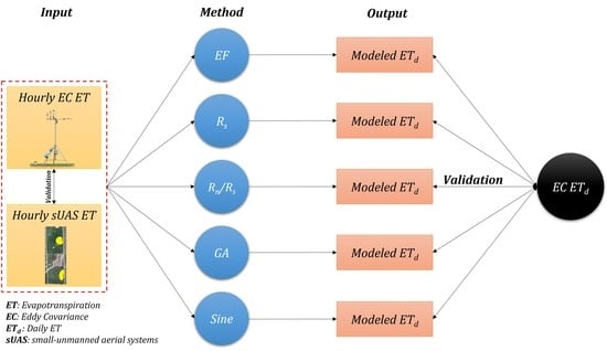
1.1. Daily ET Upscaling Approaches
1.1.1. Evaporative Fraction (EF) Approach
1.1.2. Solar Radiation (Rs) Approach
1.1.3. Ratio of Net Radiation-to-Solar Radiation (Rn/Rs) Approach
1.1.4. Sine Approach
1.1.5. Gaussian (GA) Approach
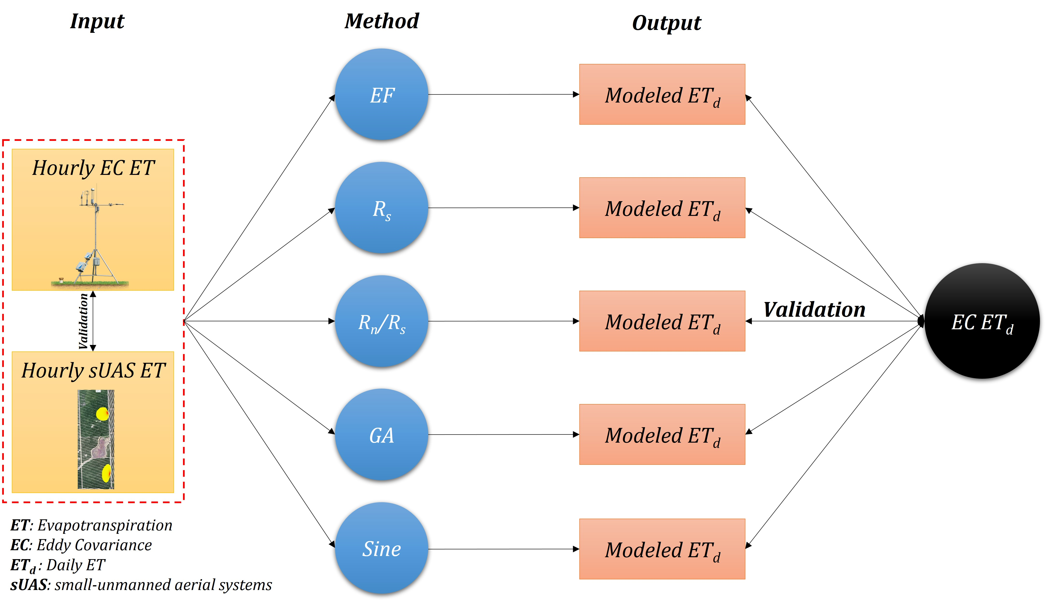
1.2. Two-Source Energy Balance (TSEB) Model

2. Methodology
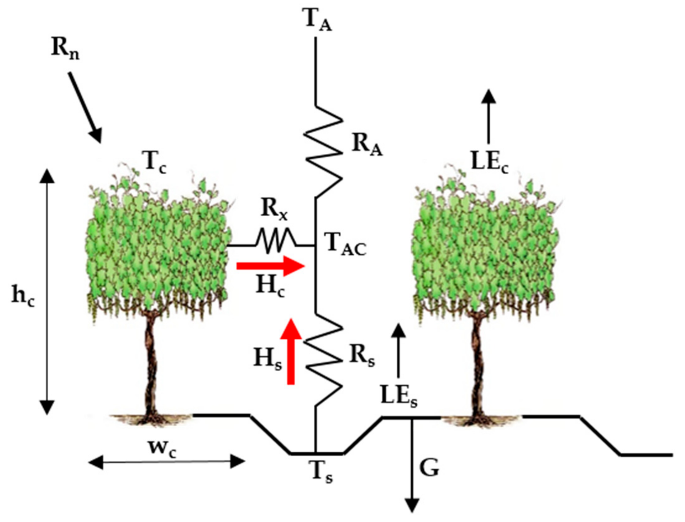
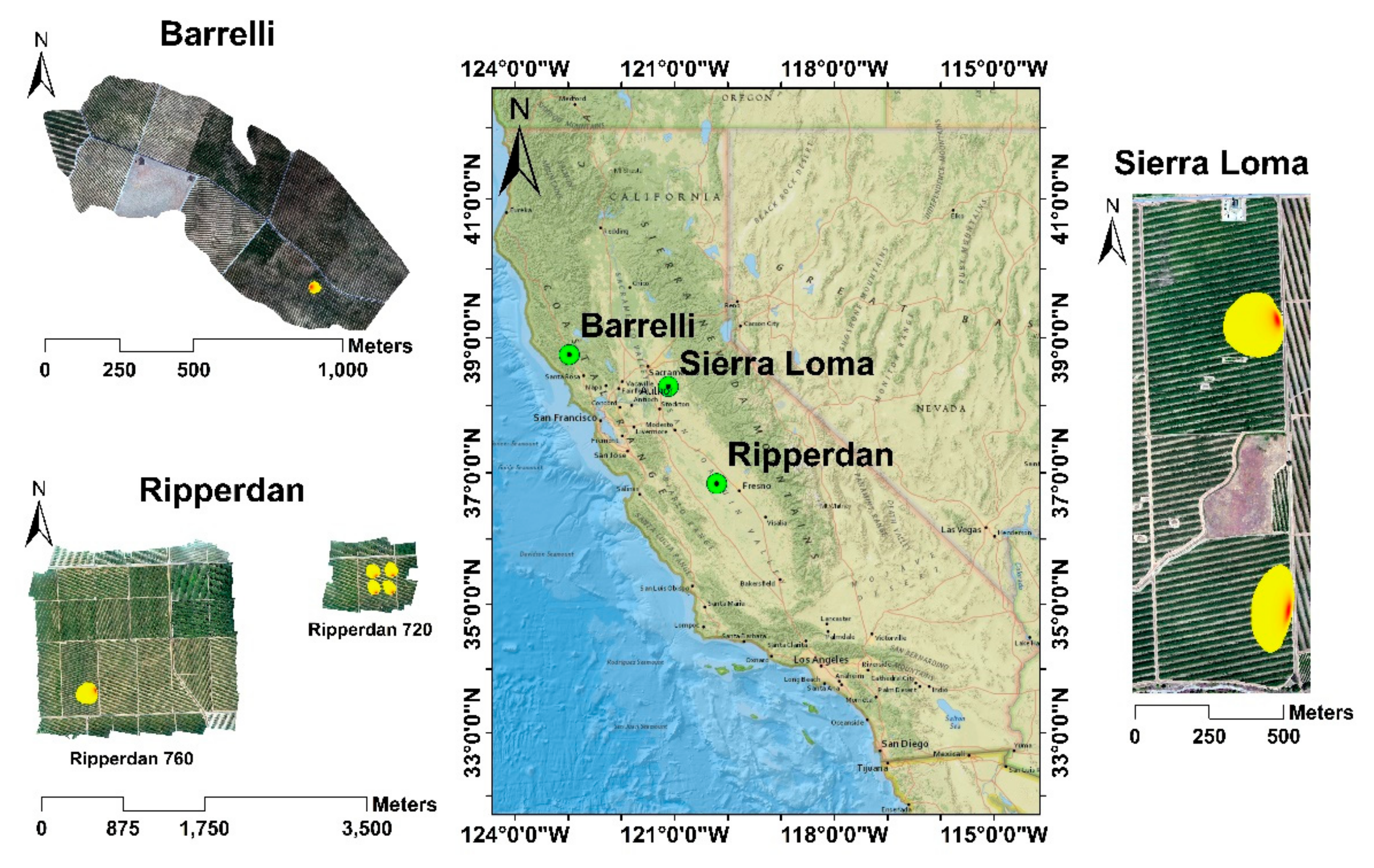
2.1. Study Area
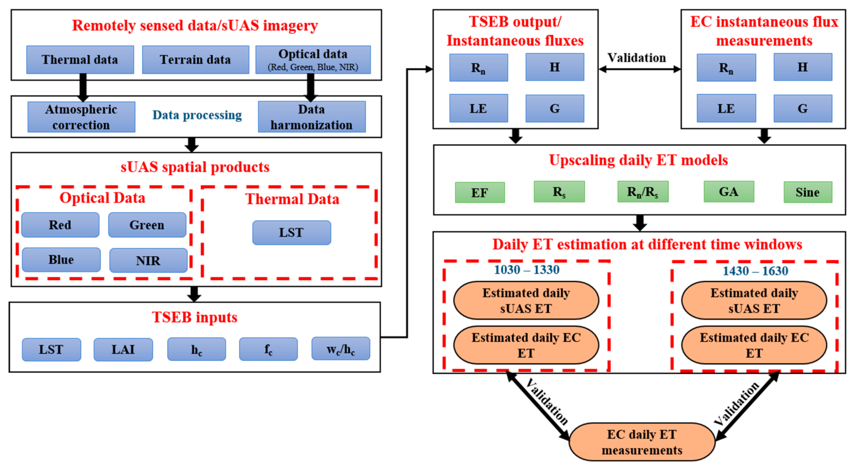
2.2. Procedure
2.2.1. sUAS Data Processing
Thermal Data
Optical Data
2.2.2. Eddy Covariance (EC) Fluxes
2.3. Goodness-of-Fit Statistics
2.3.1. Quantitative Statistics
2.3.2. Graphical Representations
3. Results and Discussion
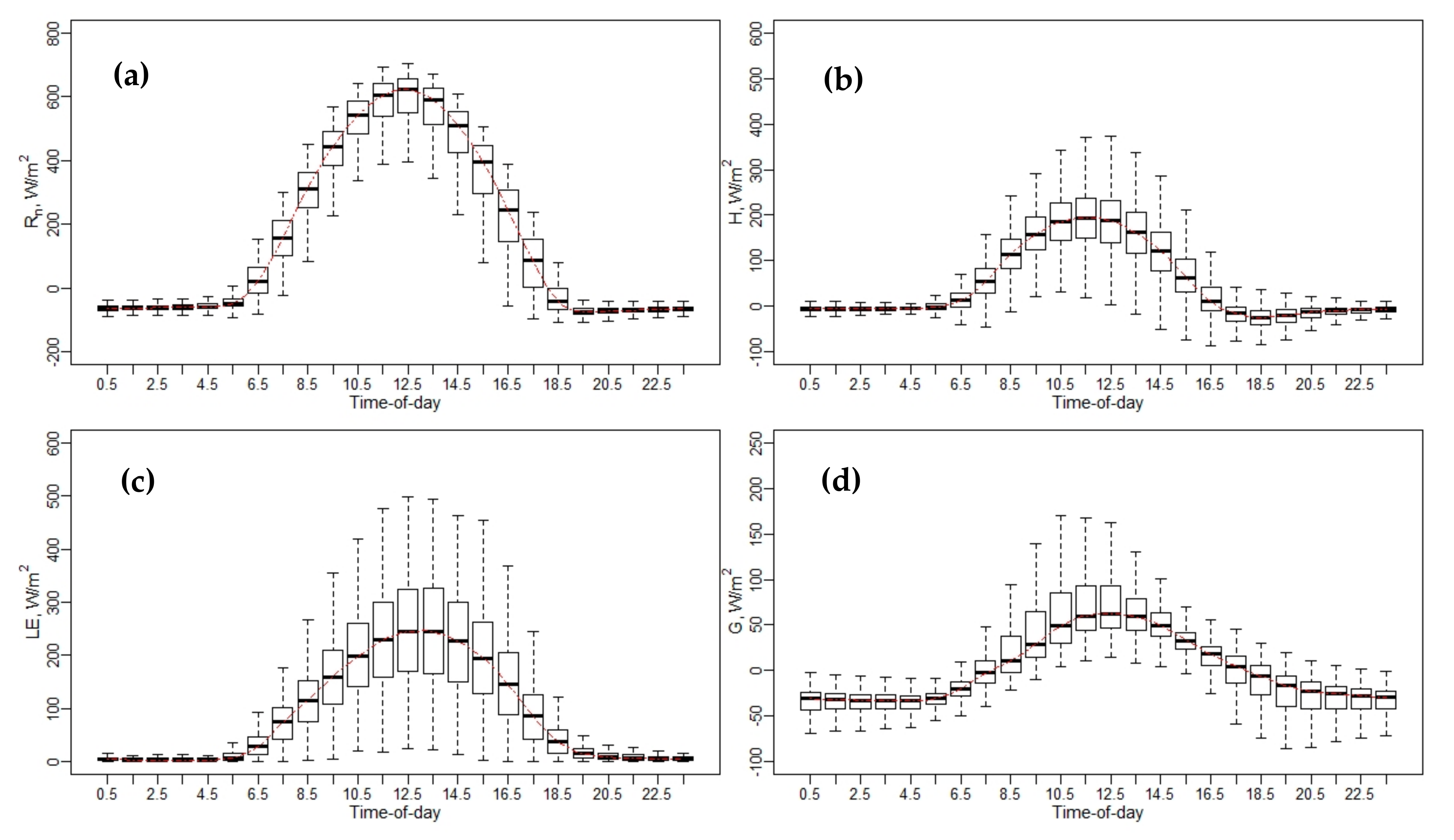
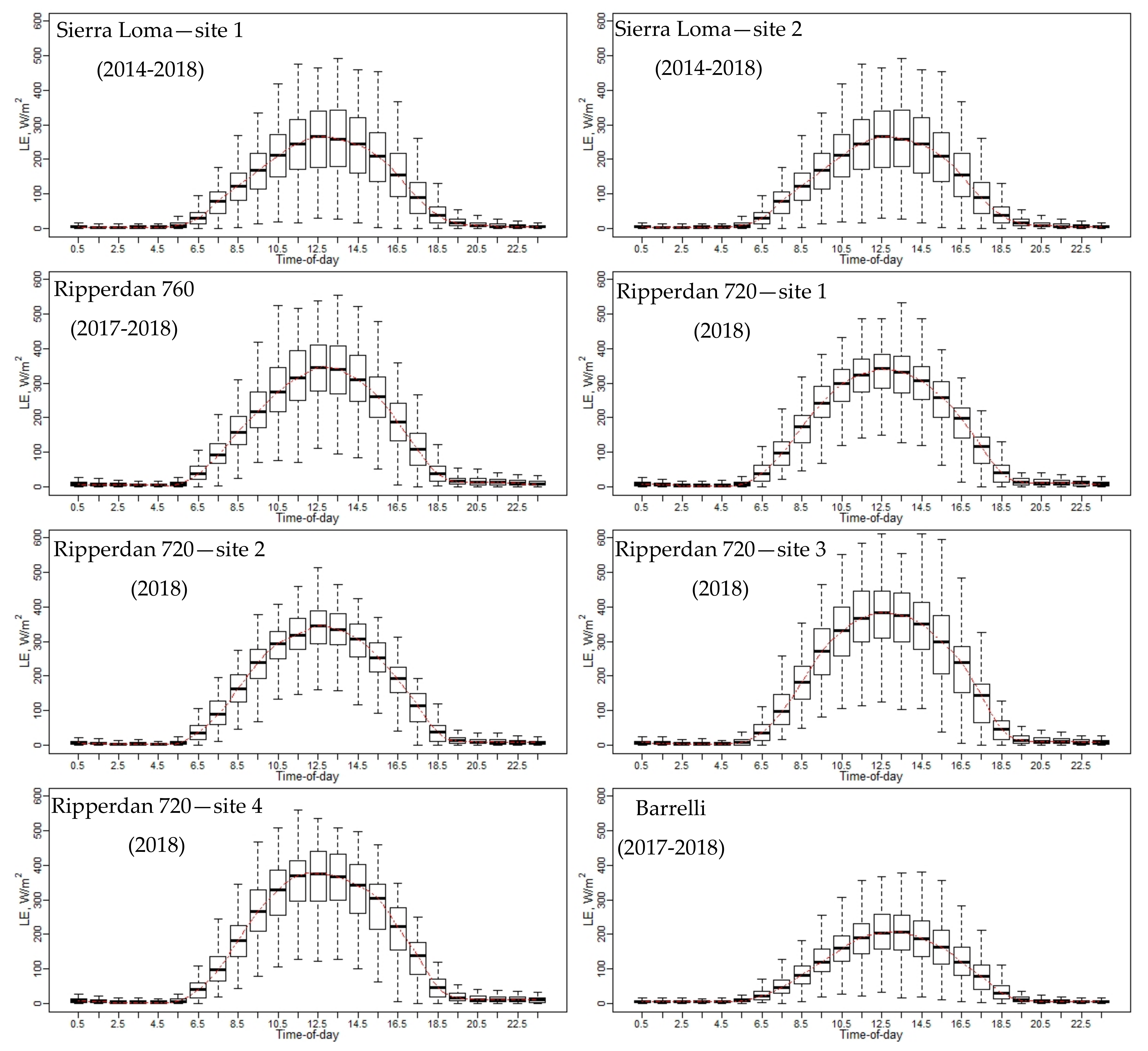
3.1. Diurnal Variation of Energy Fluxes from EC Measurements
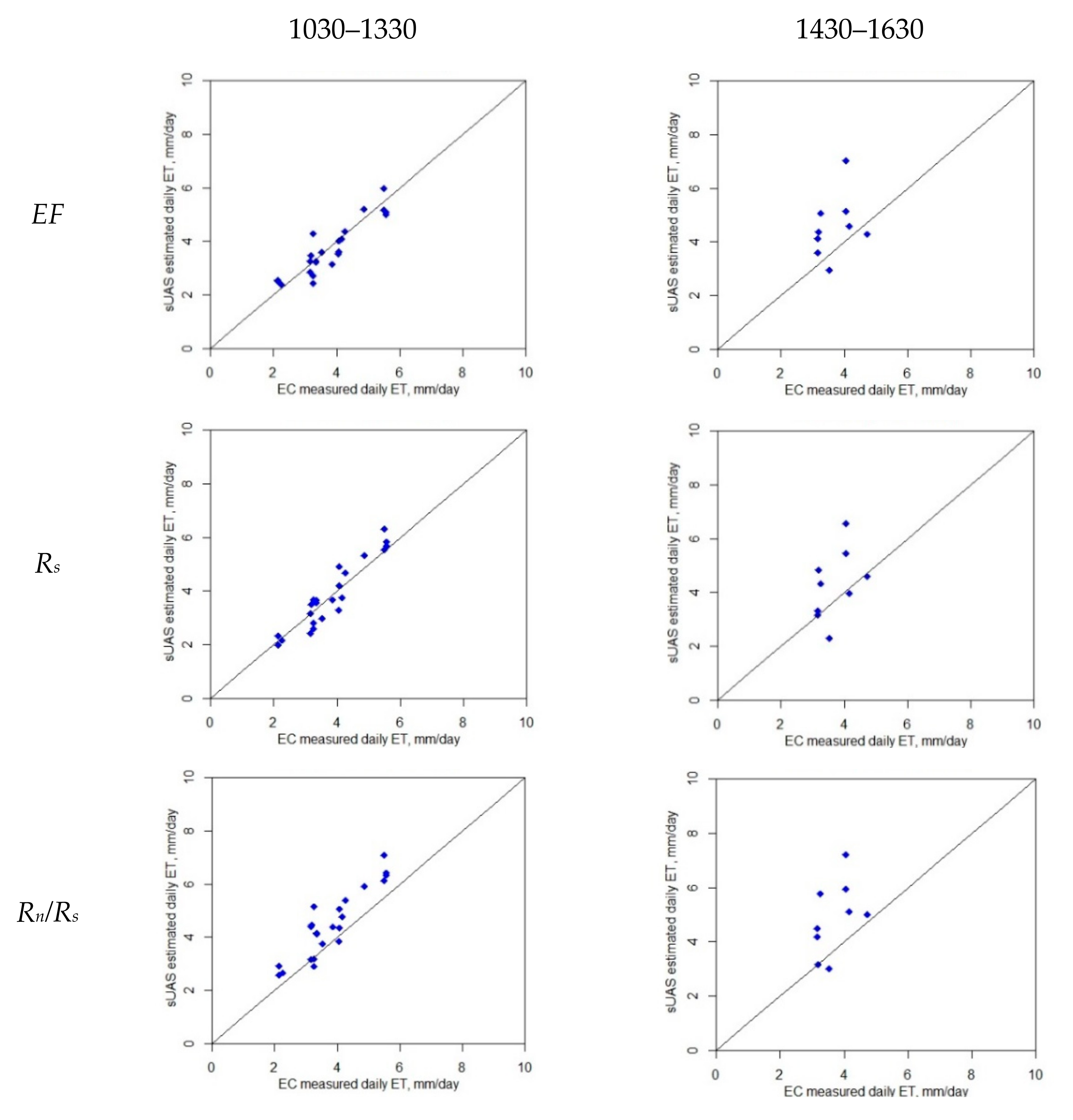
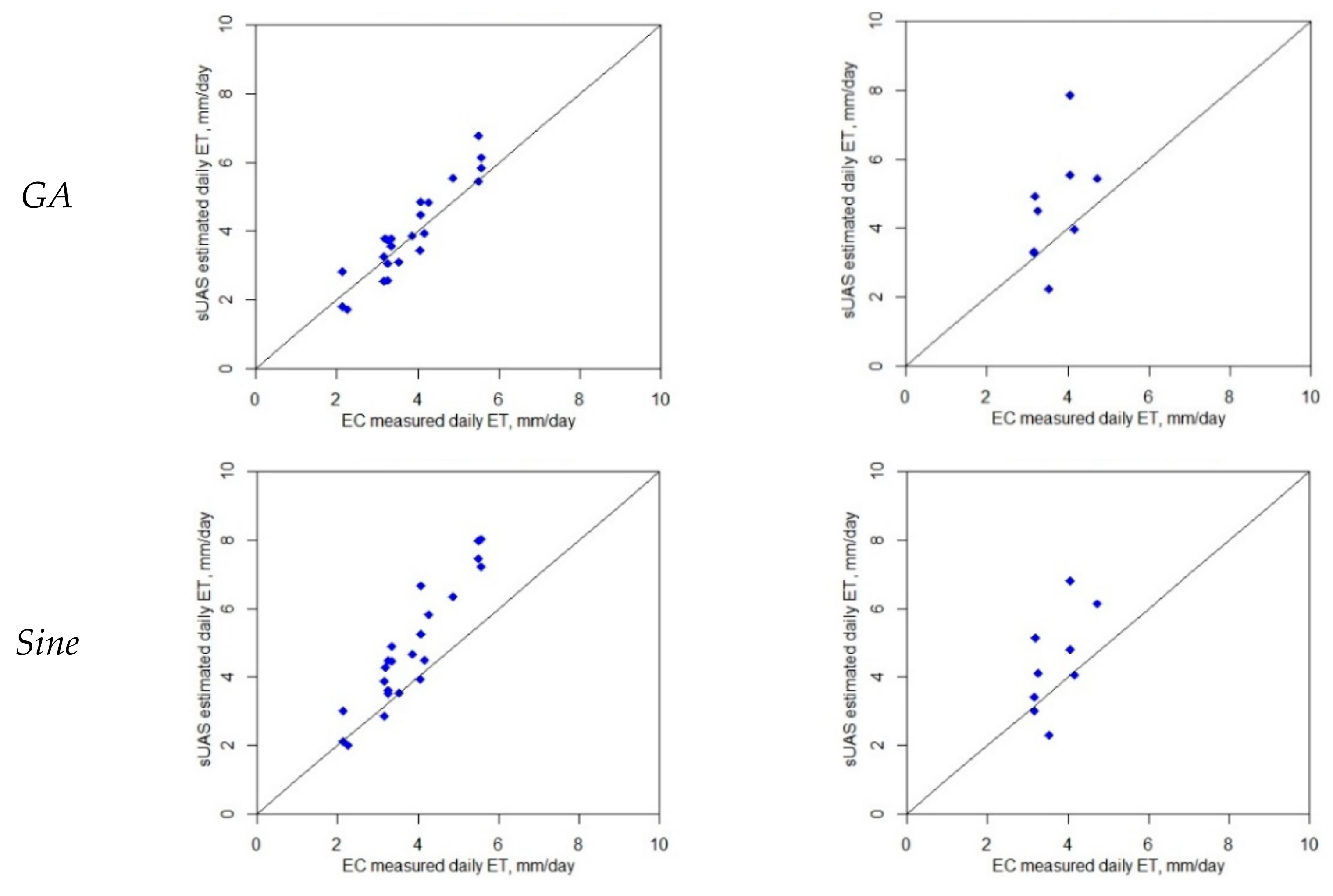
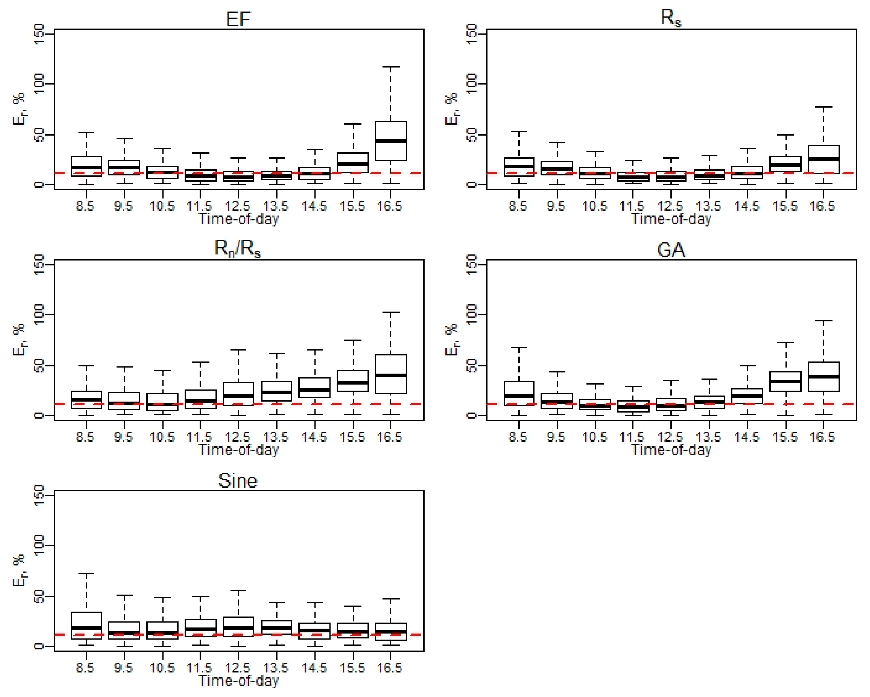
3.2. Comparison between Different ETd Extrapolation Approaches Using the EC Measurements
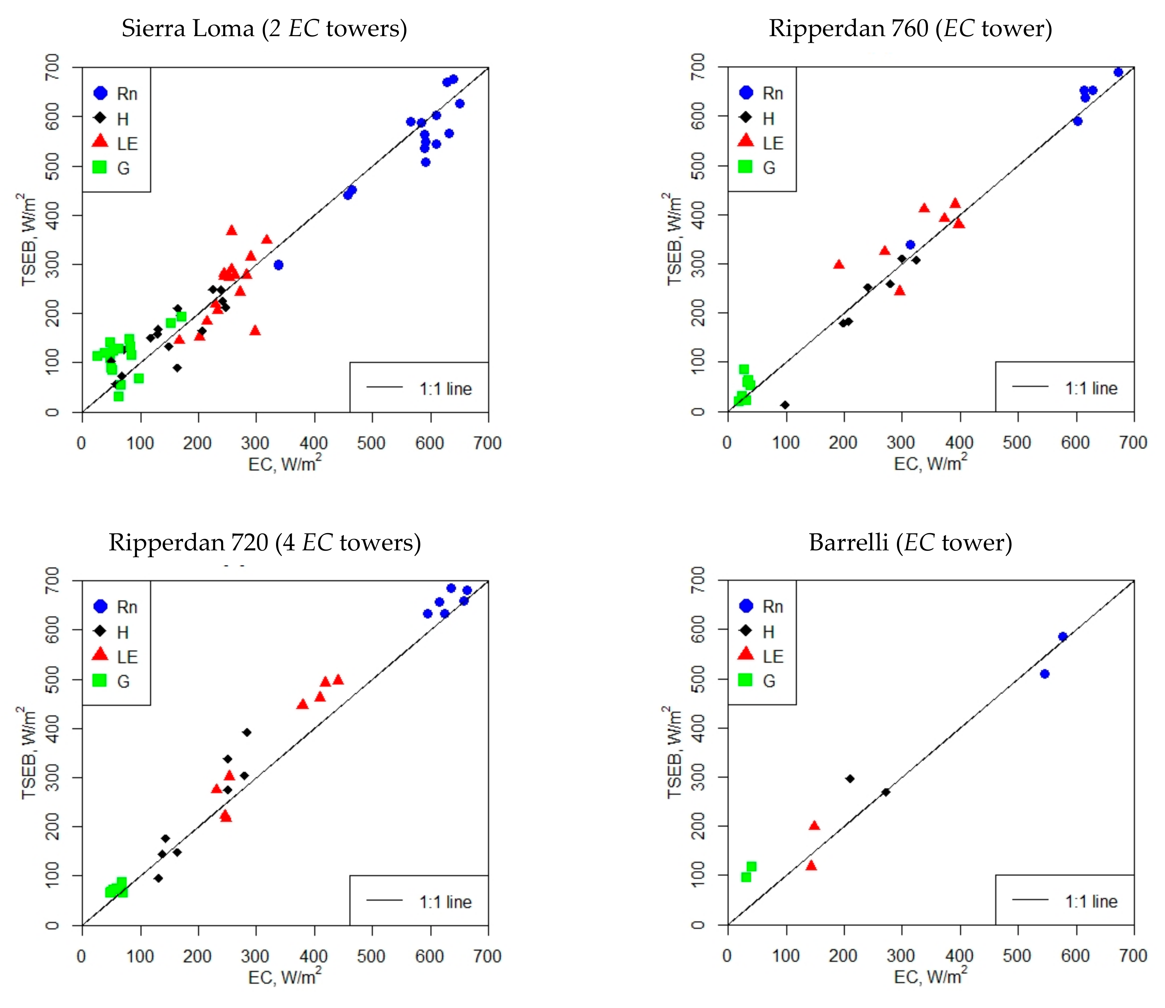
3.3. Assessing the Instantaneous TSEB ET versus EC Measurements
3.4. Assessment of the Daily ET Extrapolation Approaches Using TSEB sUAS Results
4. Conclusions
Author Contributions
Funding
Acknowledgments
Conflicts of Interest
Appendix A. Daily ET Analysis at Sierra Loma Vineyard Near Lodi, California
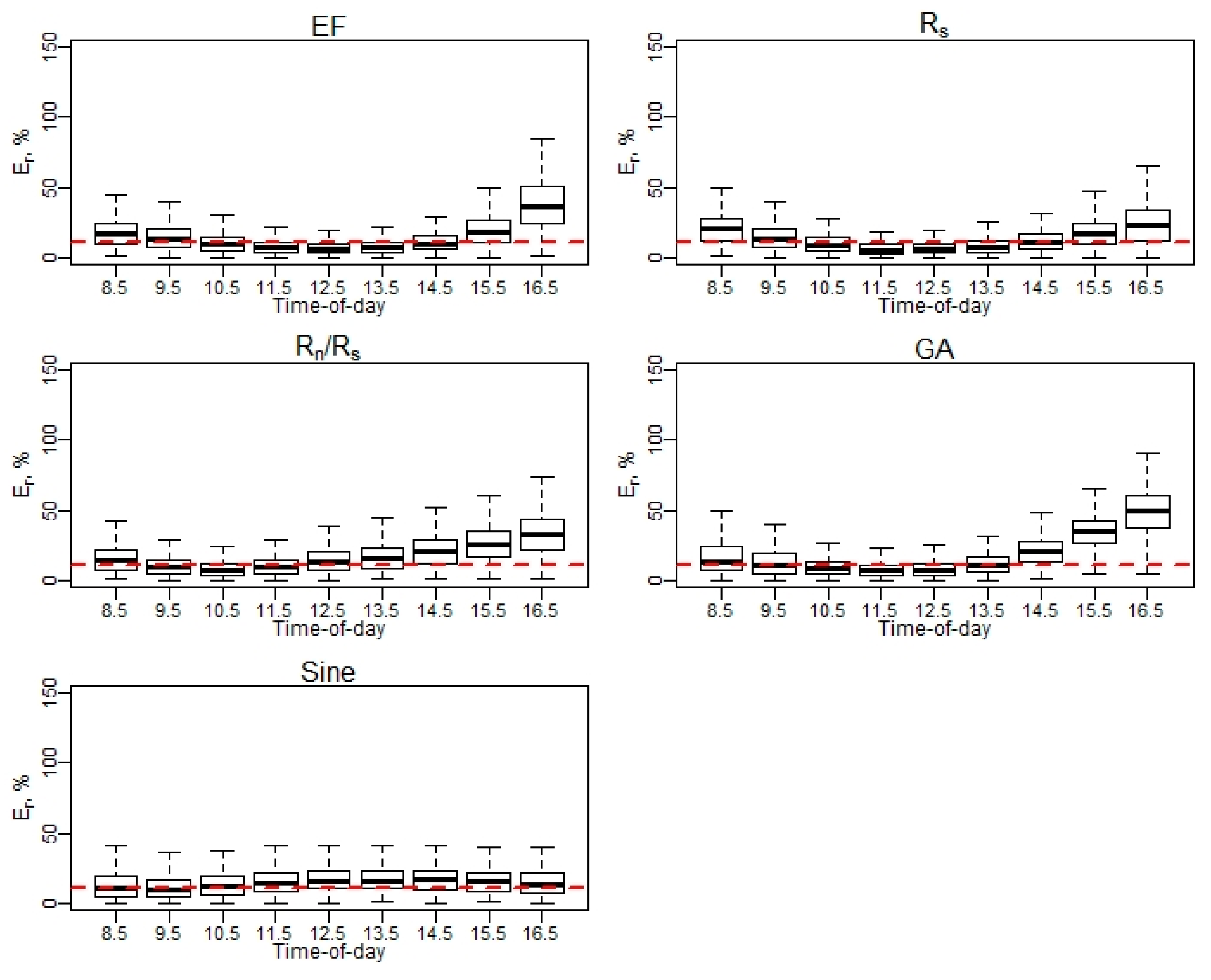
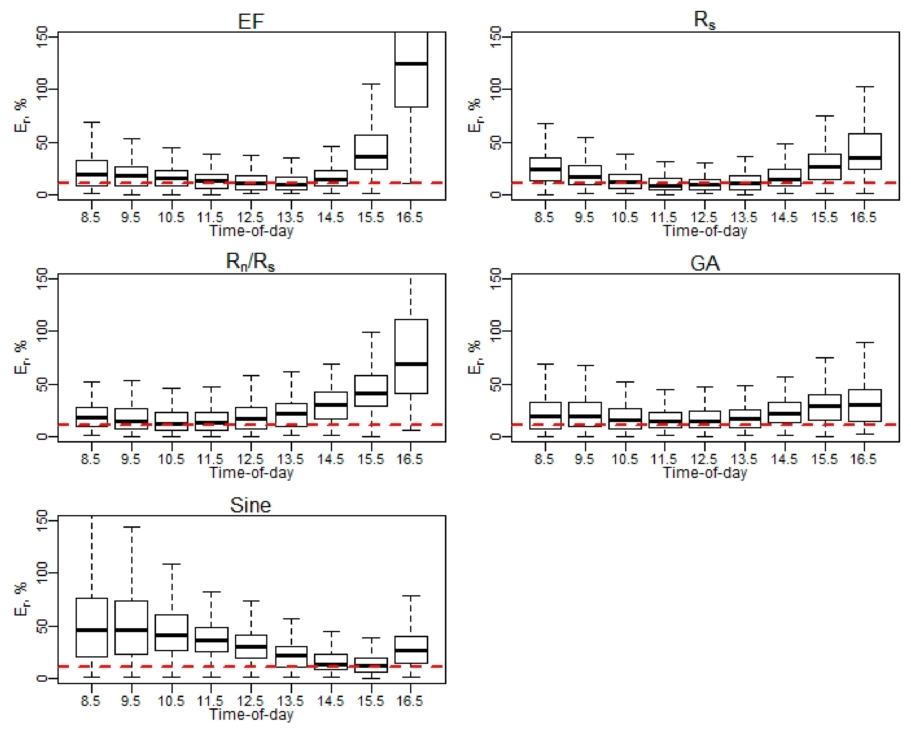
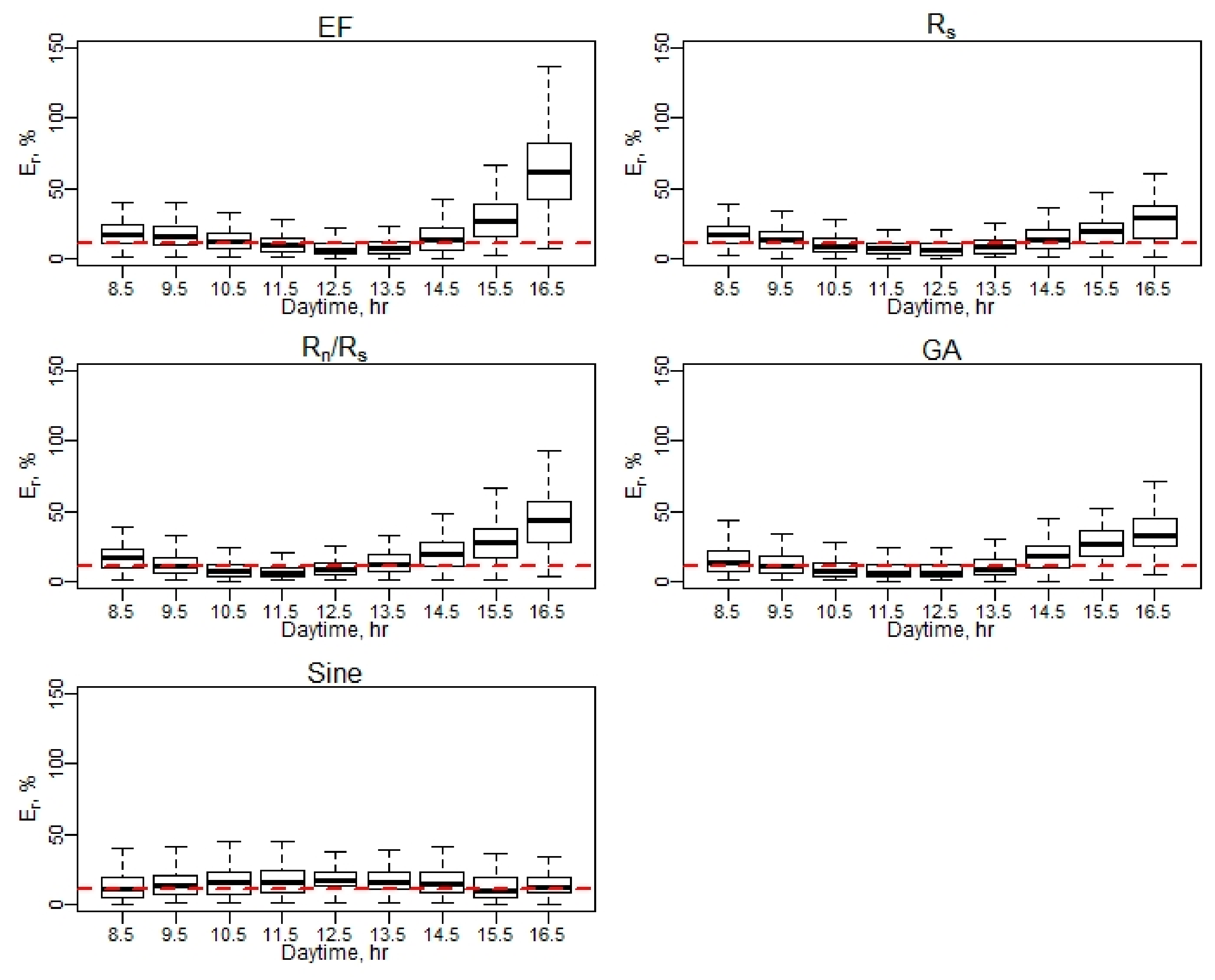
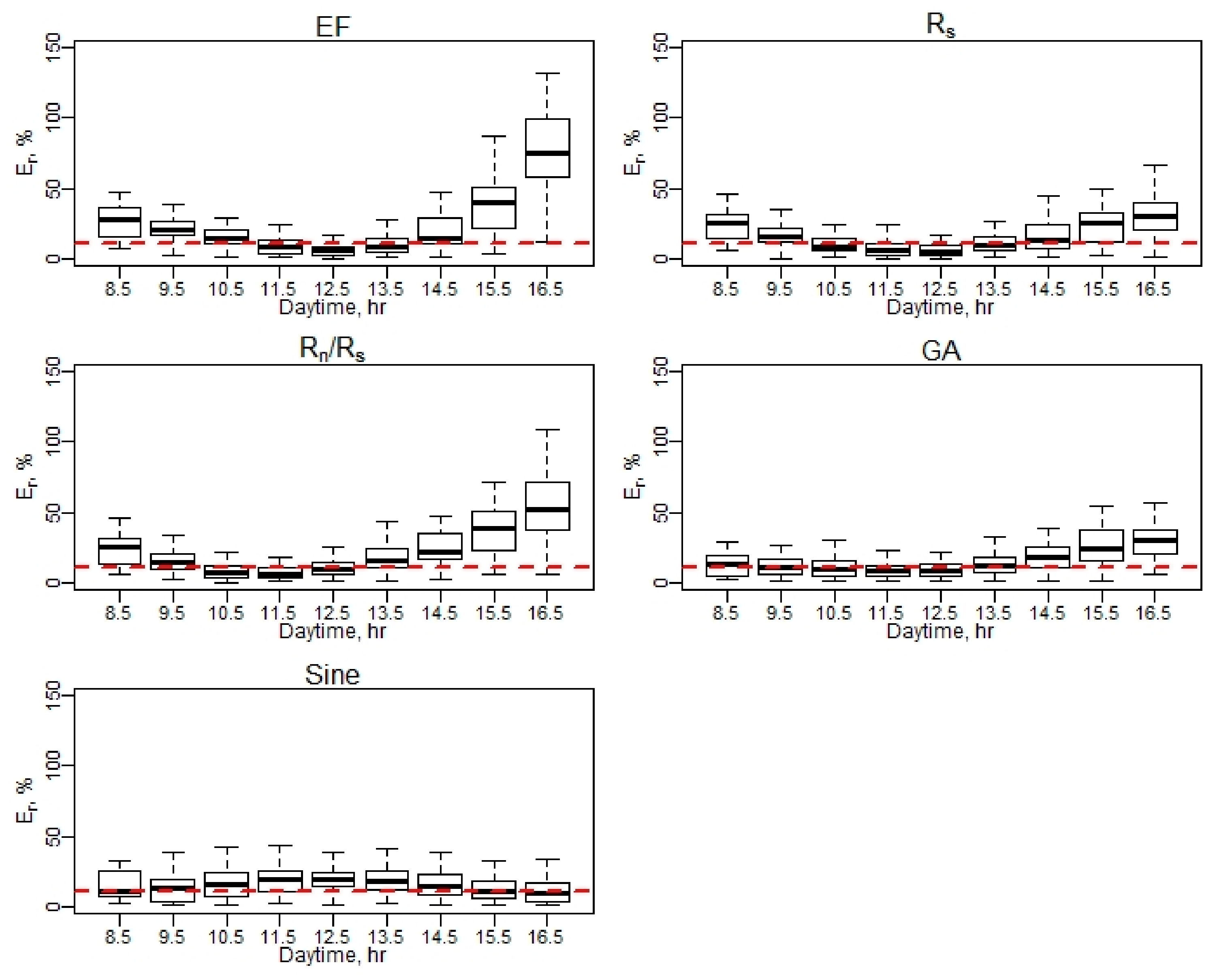
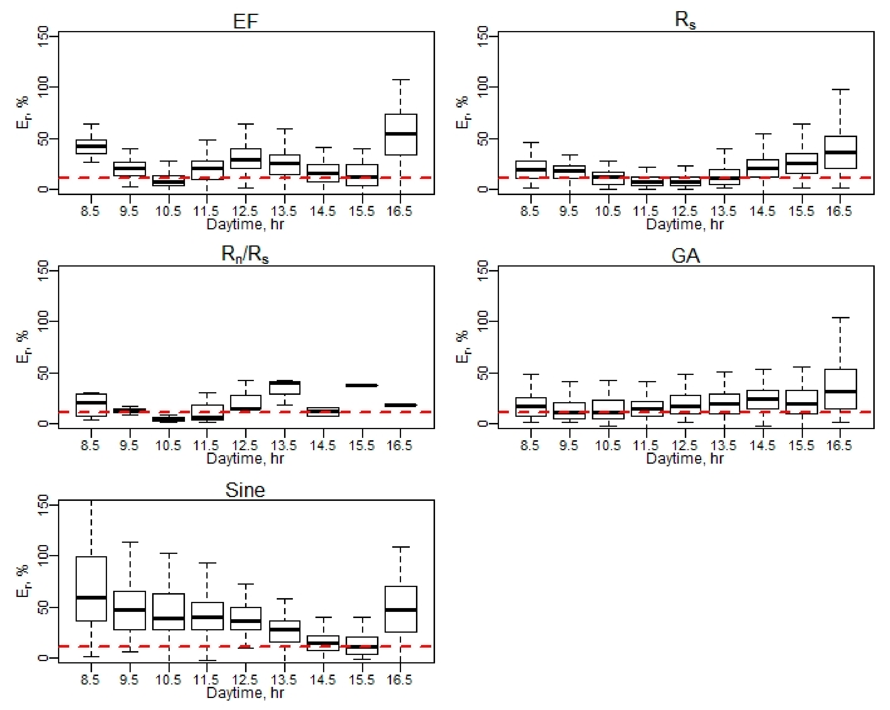
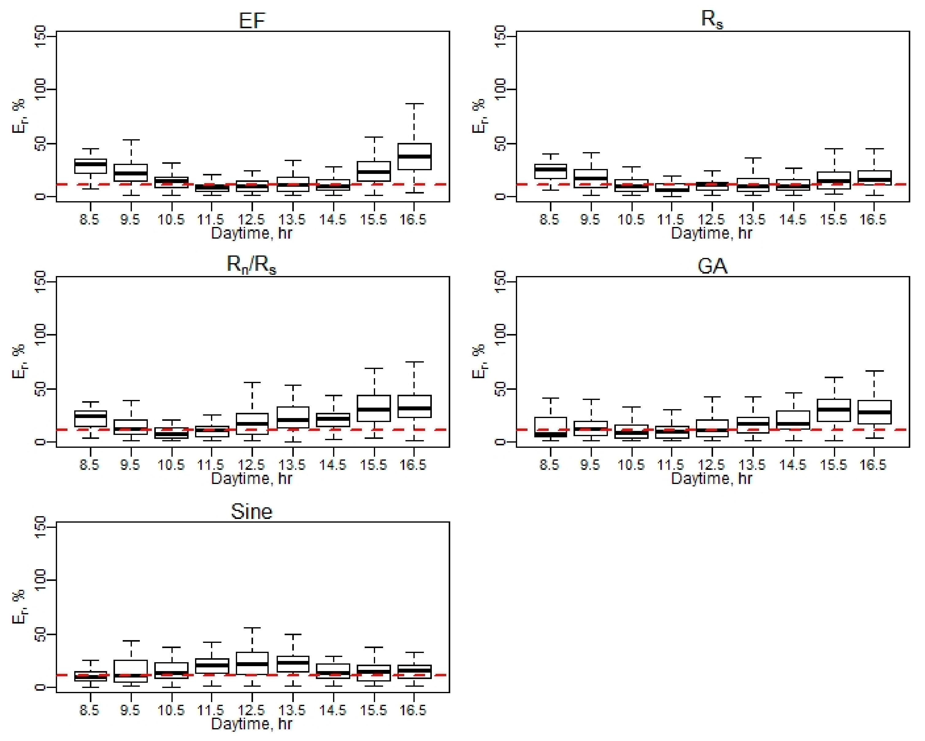
Appendix A.1. Relative Error (Er) at Hourly Scale for EC Measurements


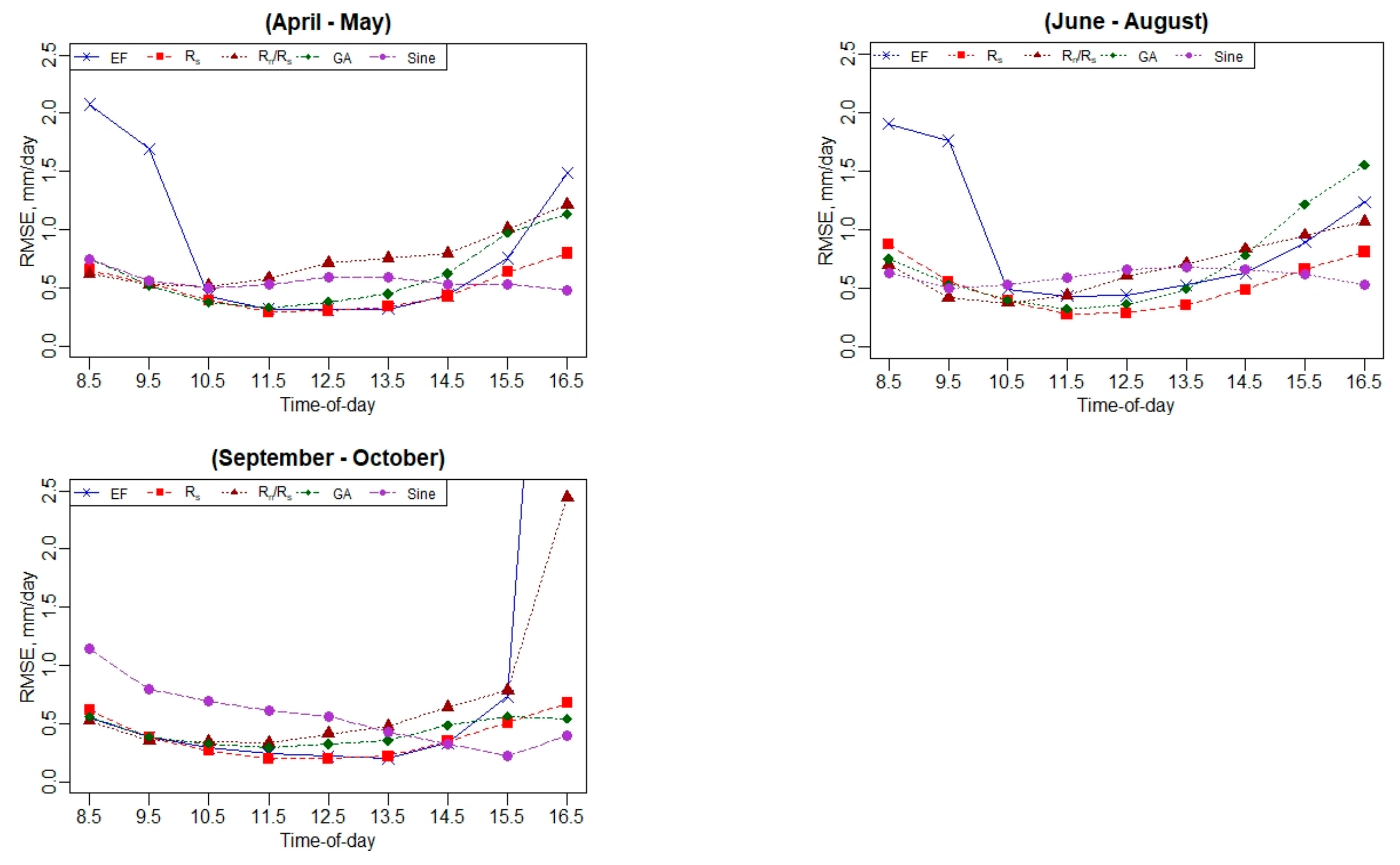
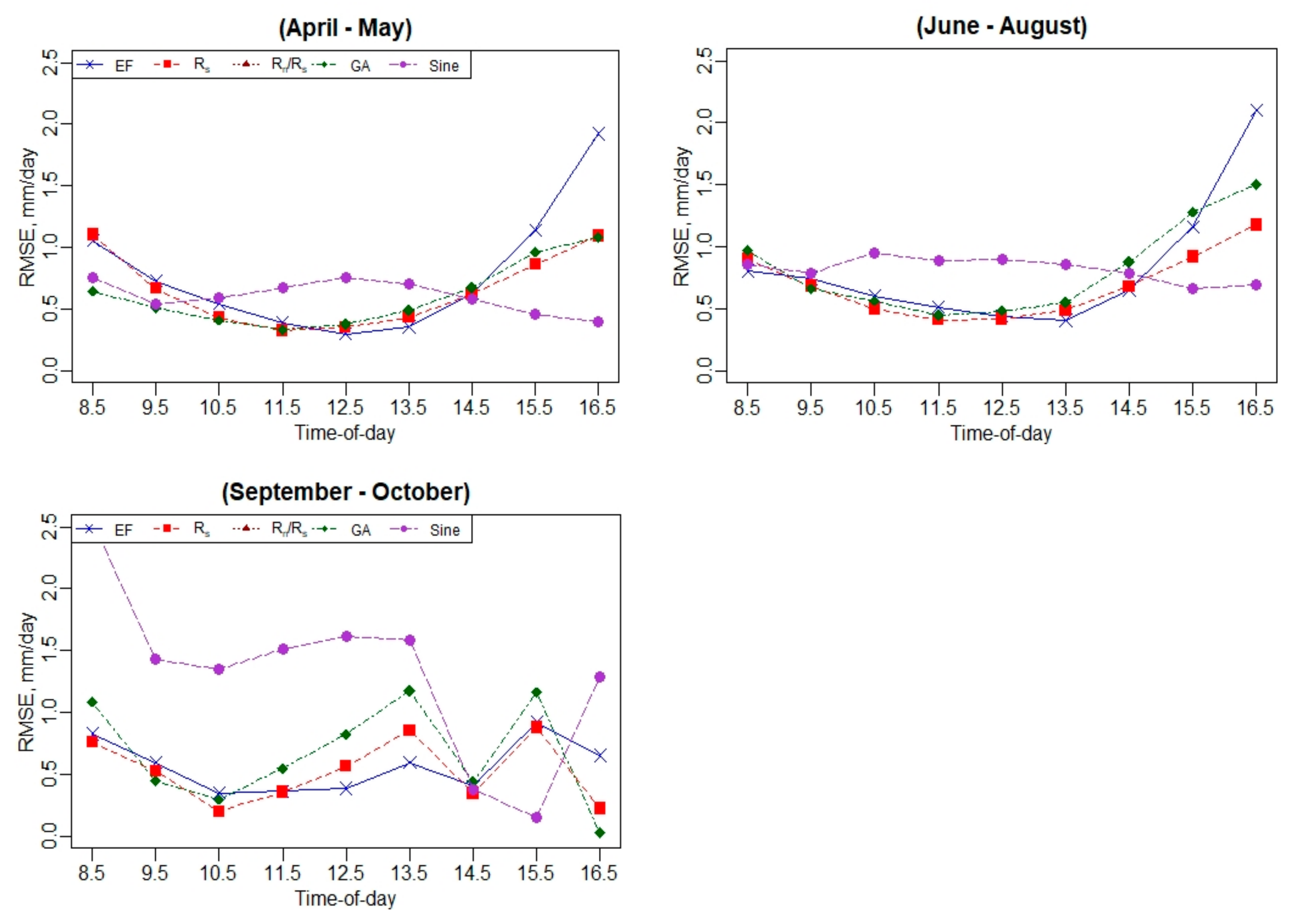
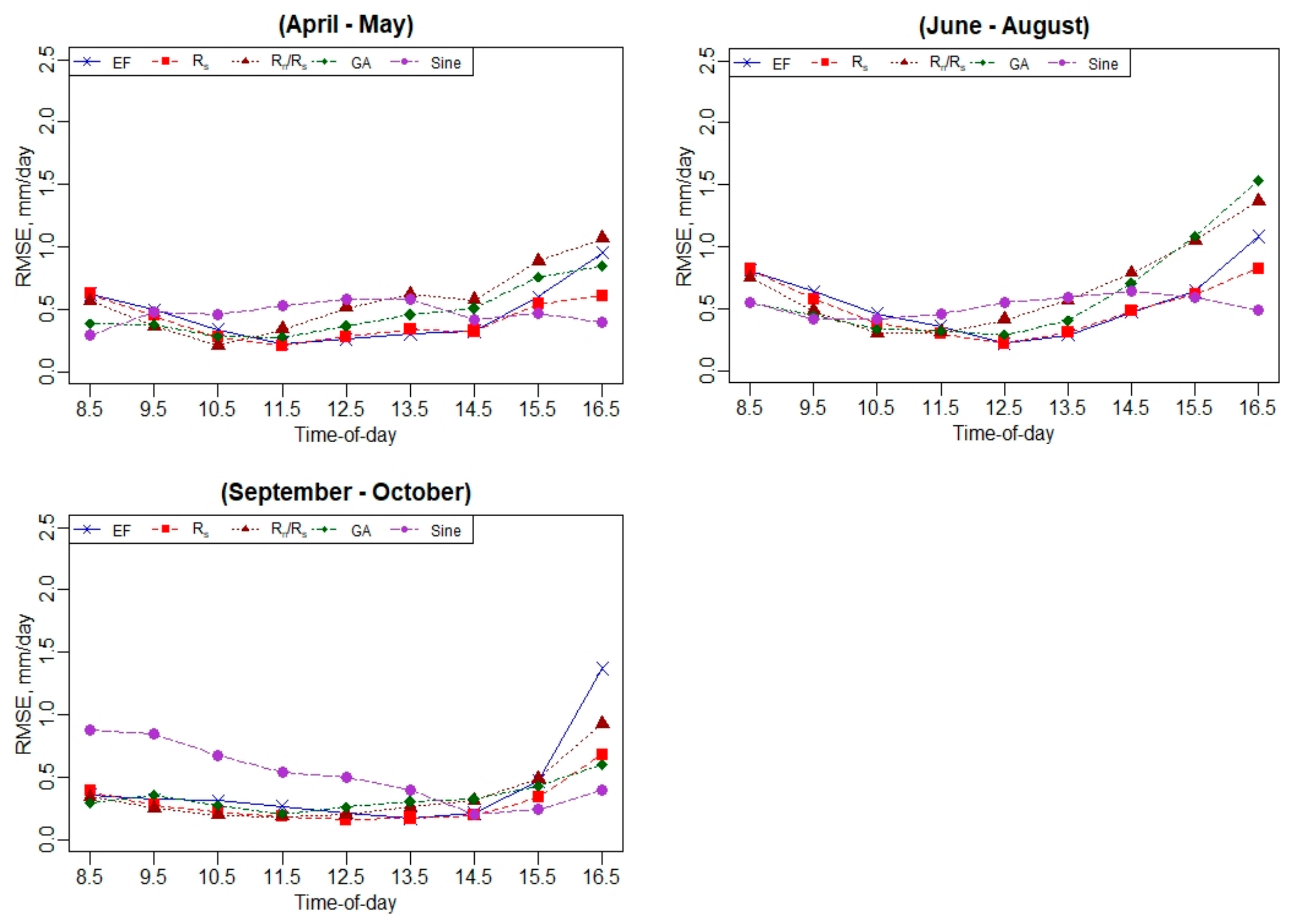
Appendix A.2. Daily RMSE Performance Using Hourly EC ET Values

Appendix B. Daily ET Analysis at Ripperdan 760 Vineyard, California
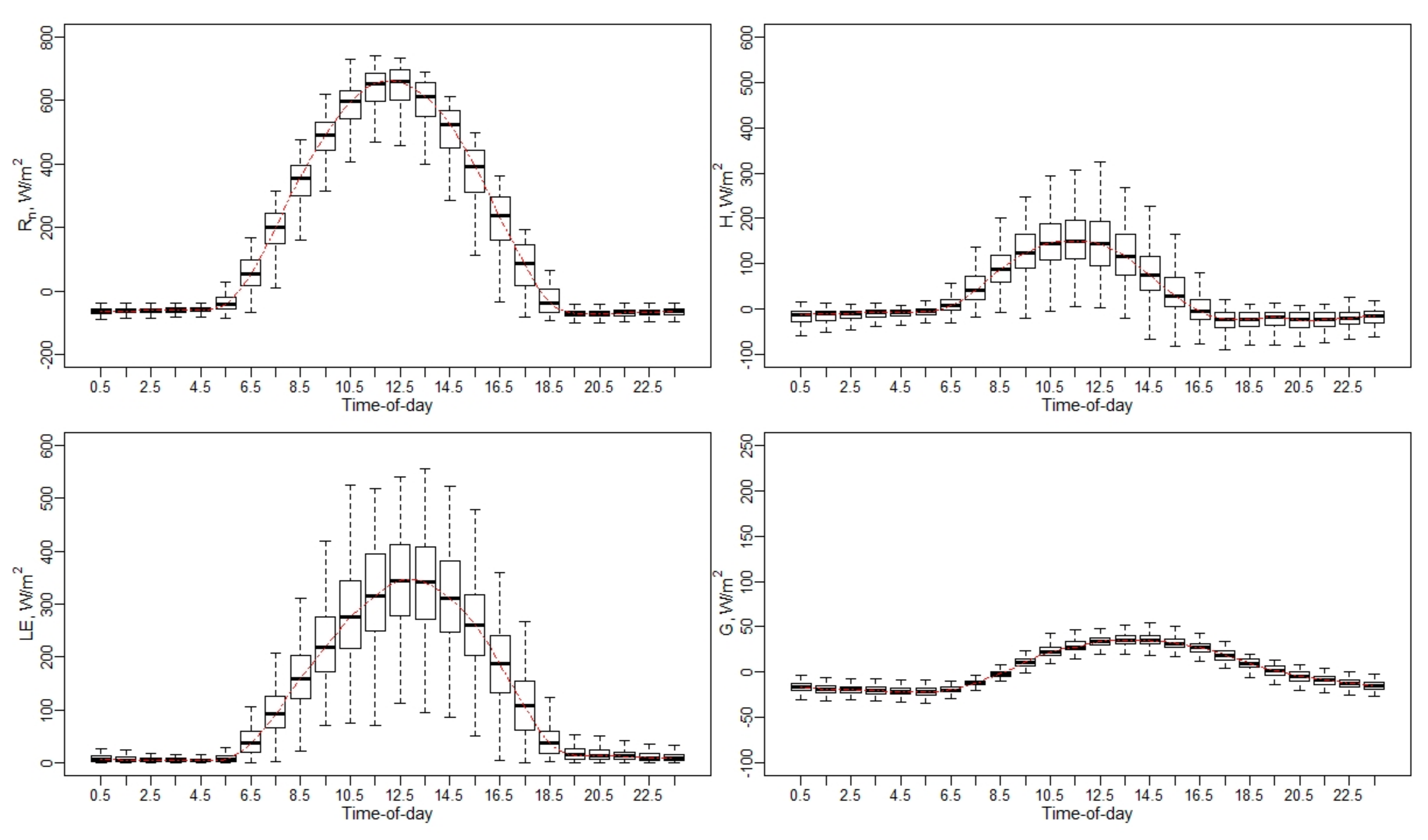
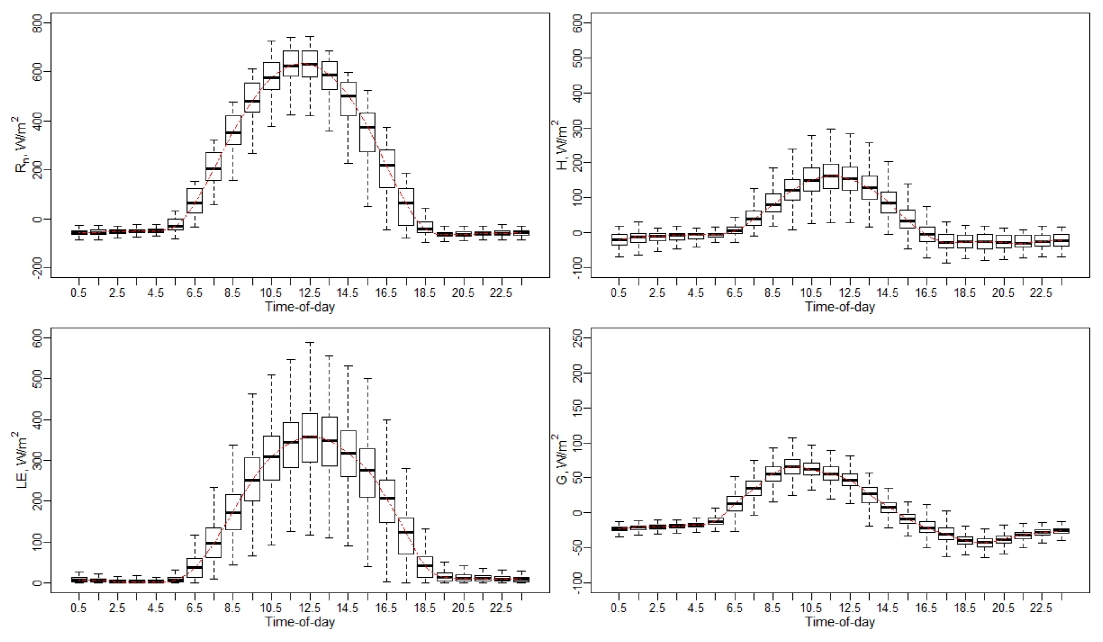
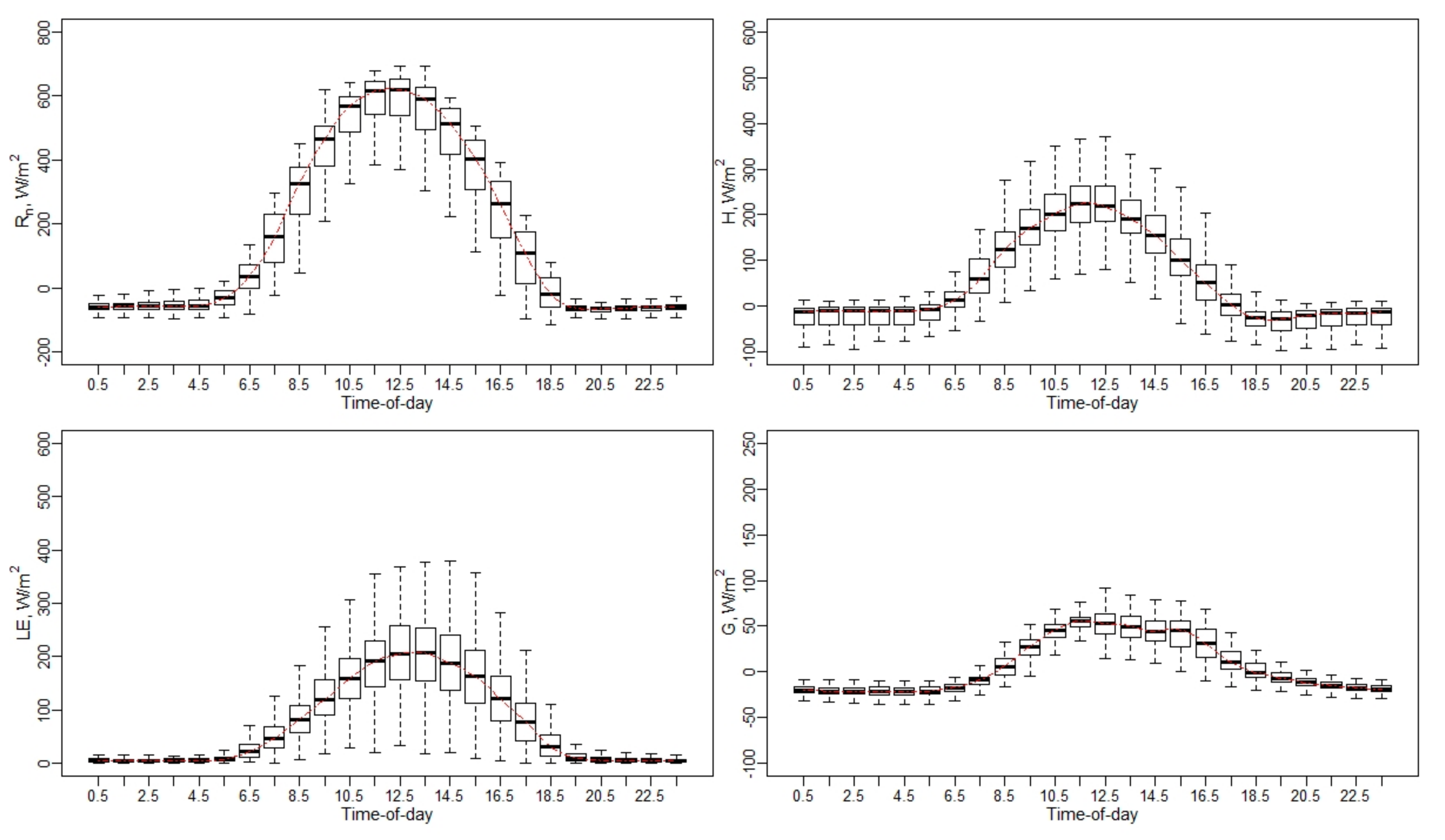
Appendix B.1. Diurnal Variation of Surface Energy Fluxes (Rn, H, LE, and G)

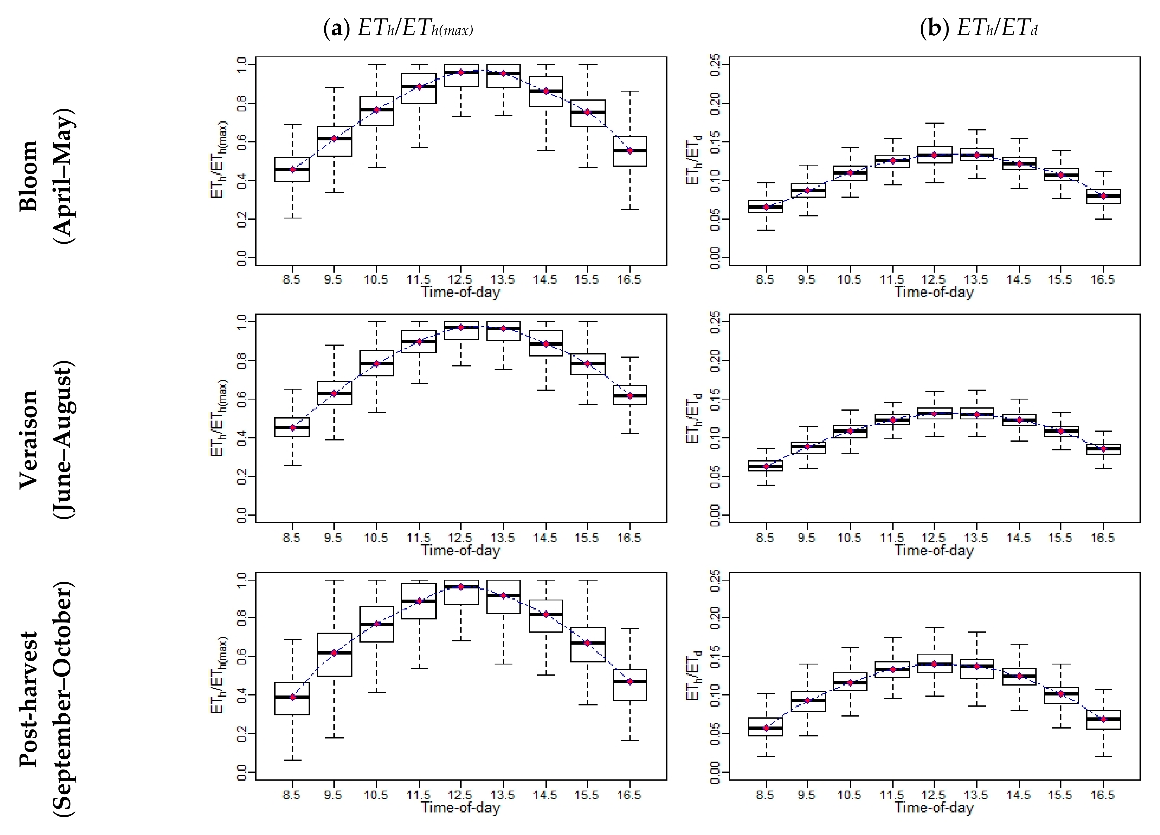
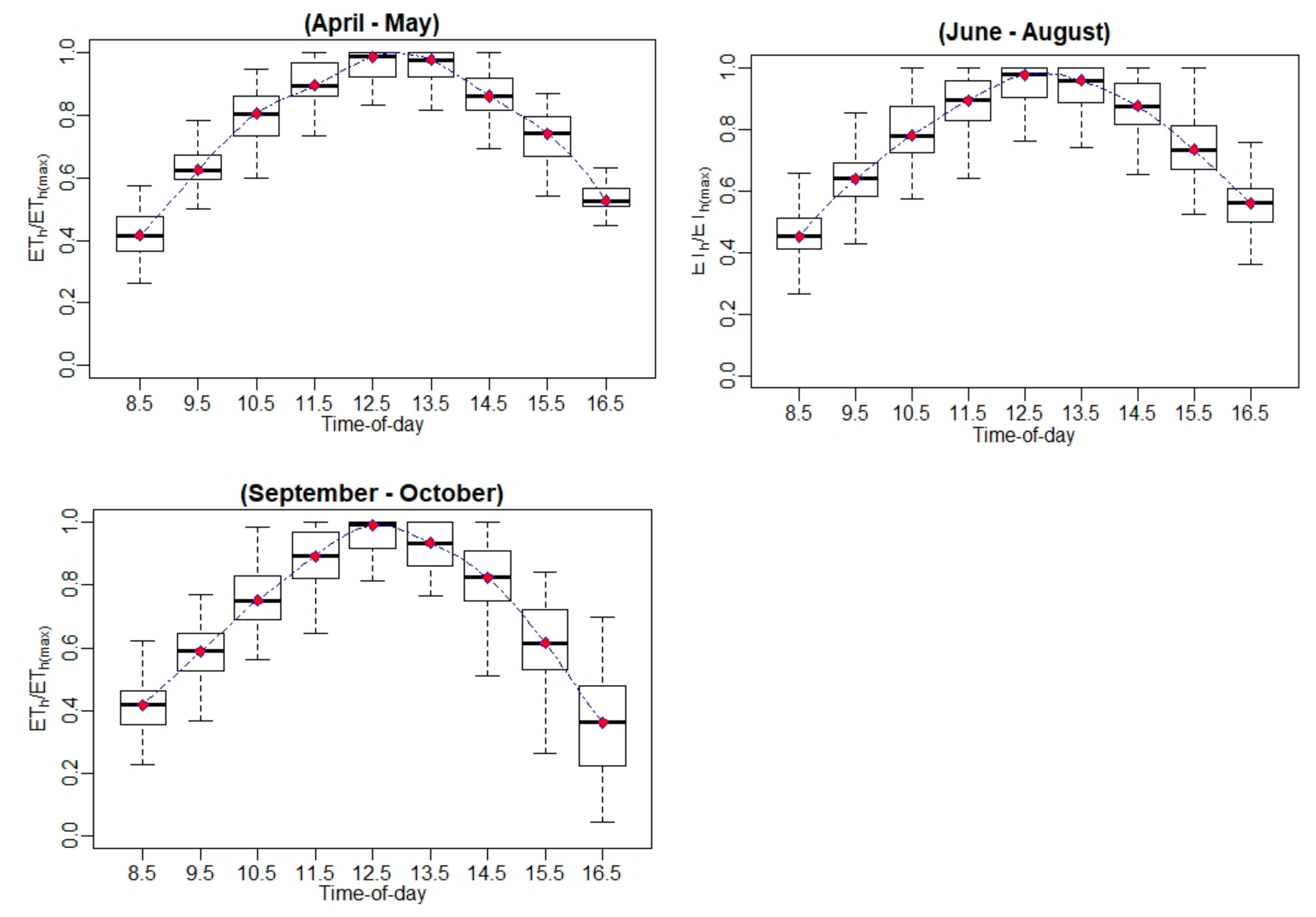
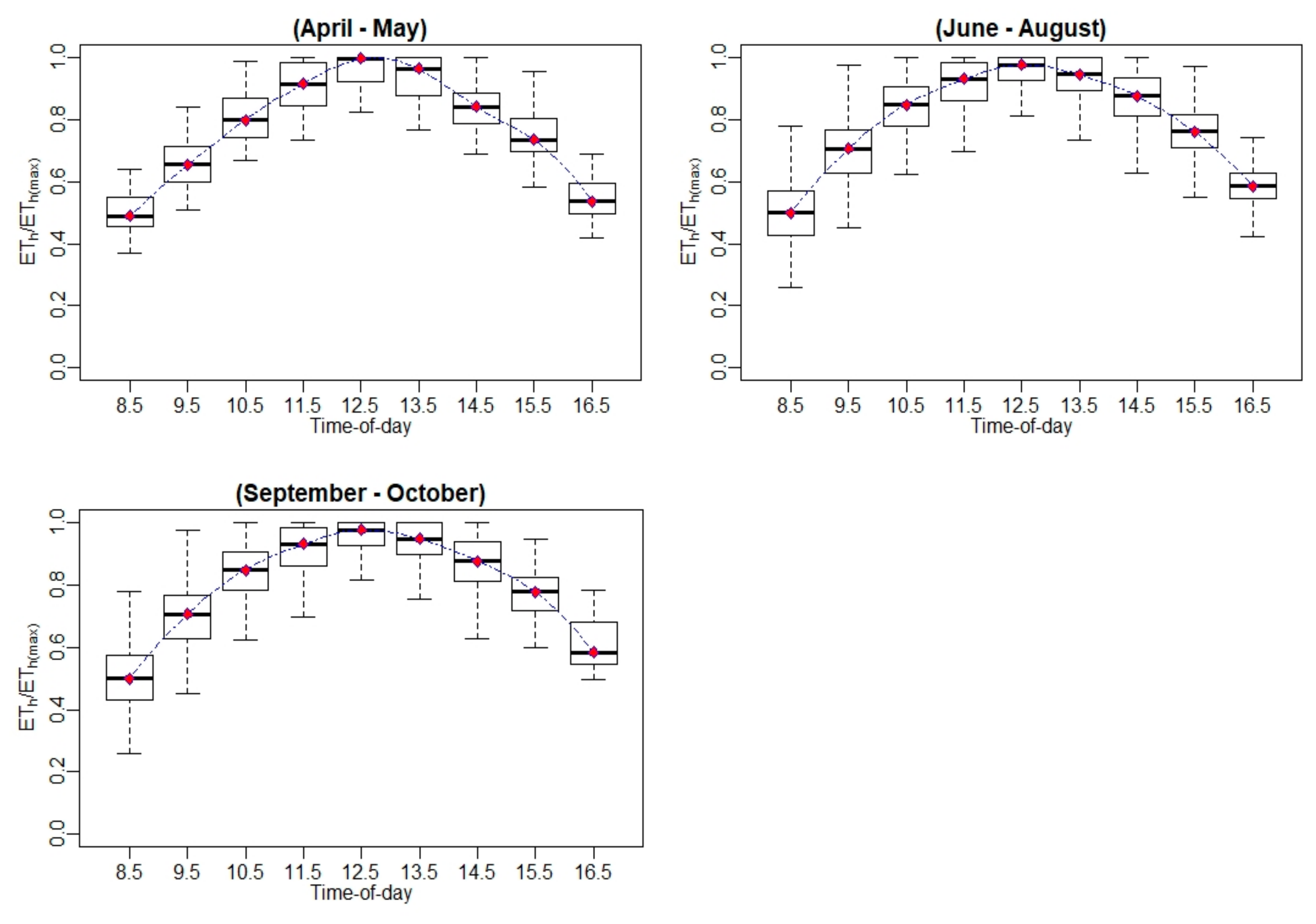
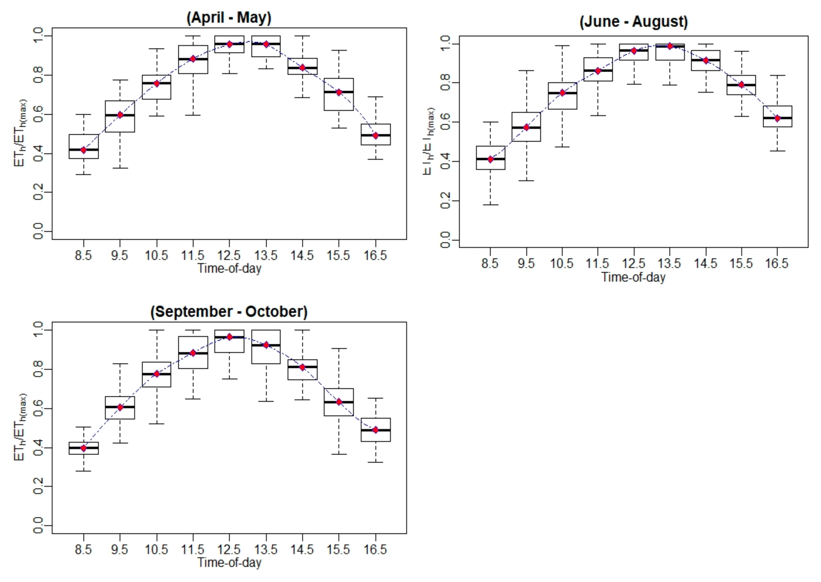
Appendix B.2. Hourly ET to Maximum Hourly ET Ratio (ETh/ETh(max)) Variation Using EC Measurements

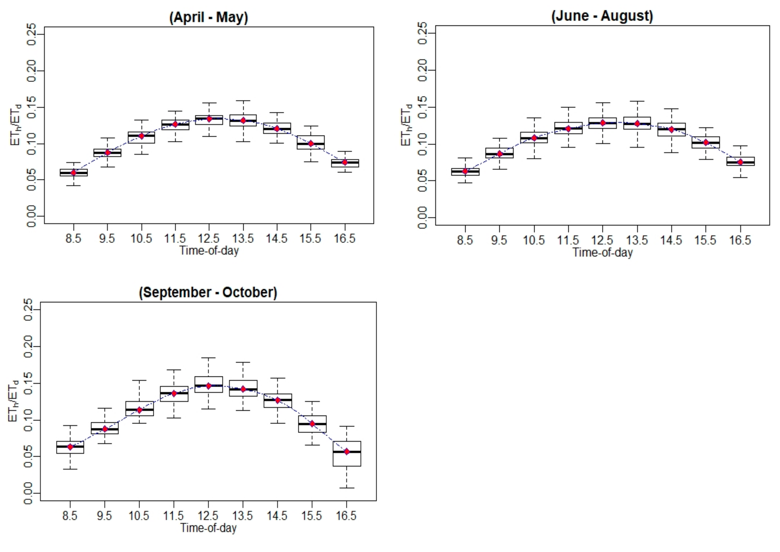
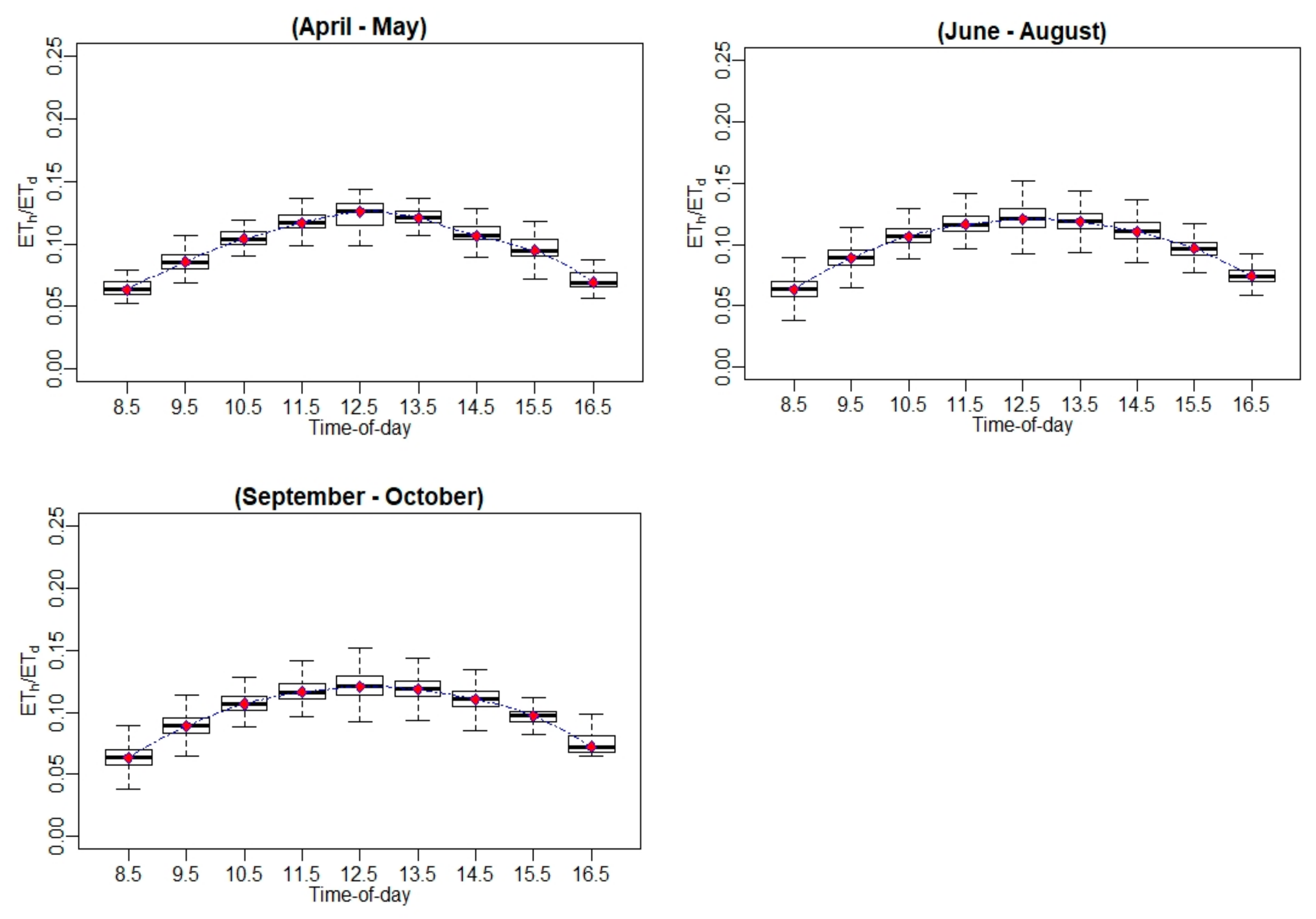
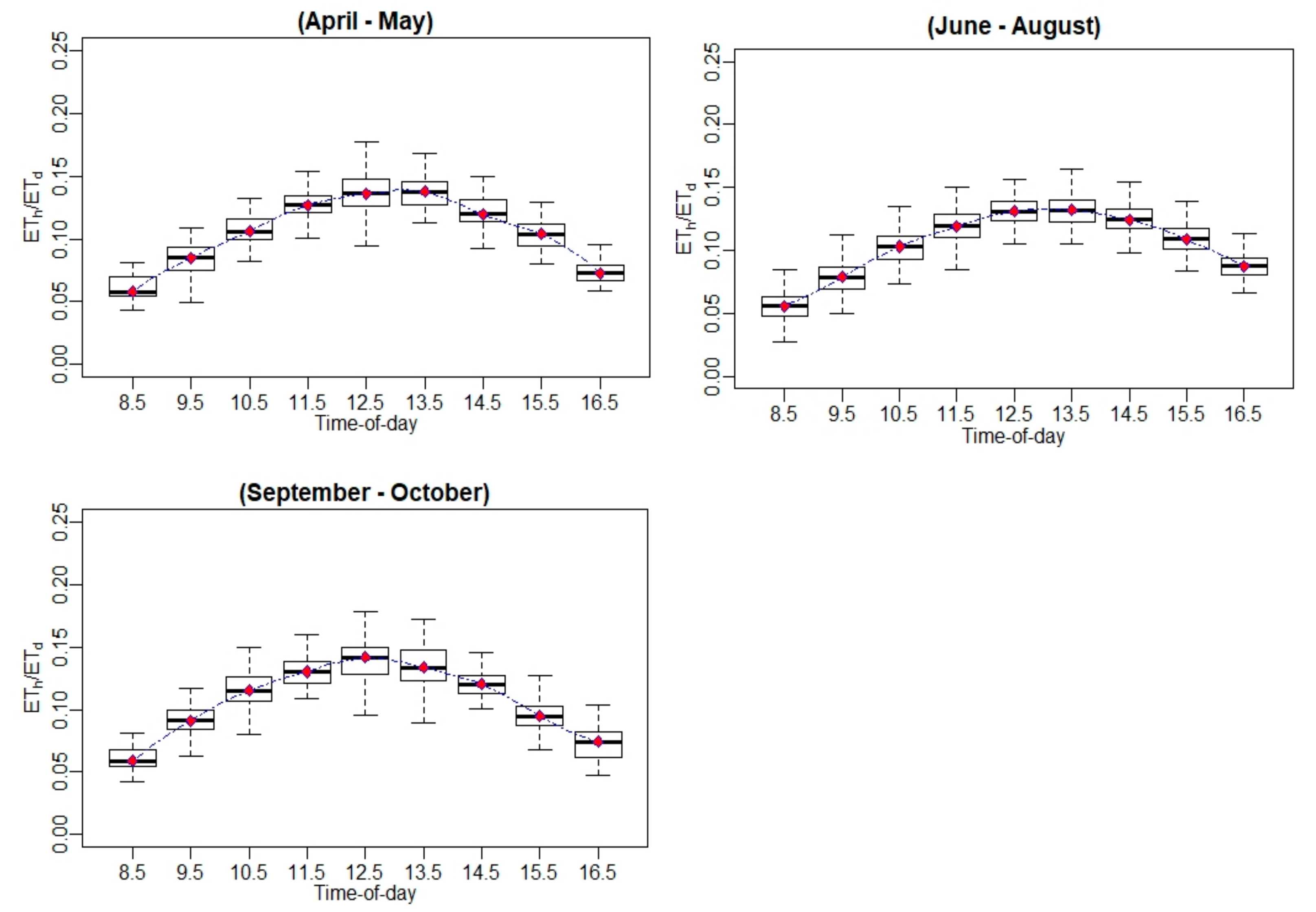
Appendix B.3. Hourly ET-to-Daily ET Ratio (ETh/ETd) variation Using EC Measurements

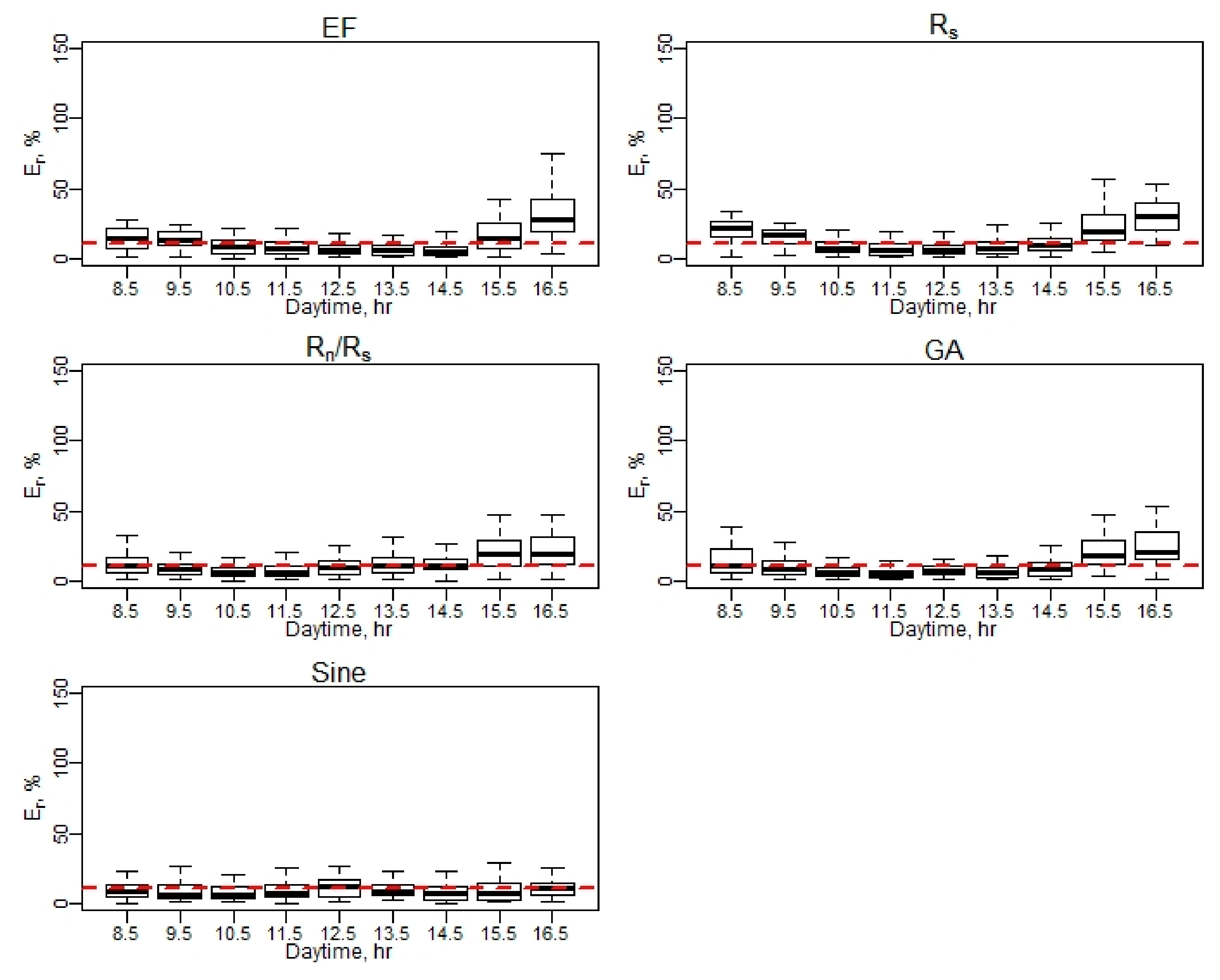
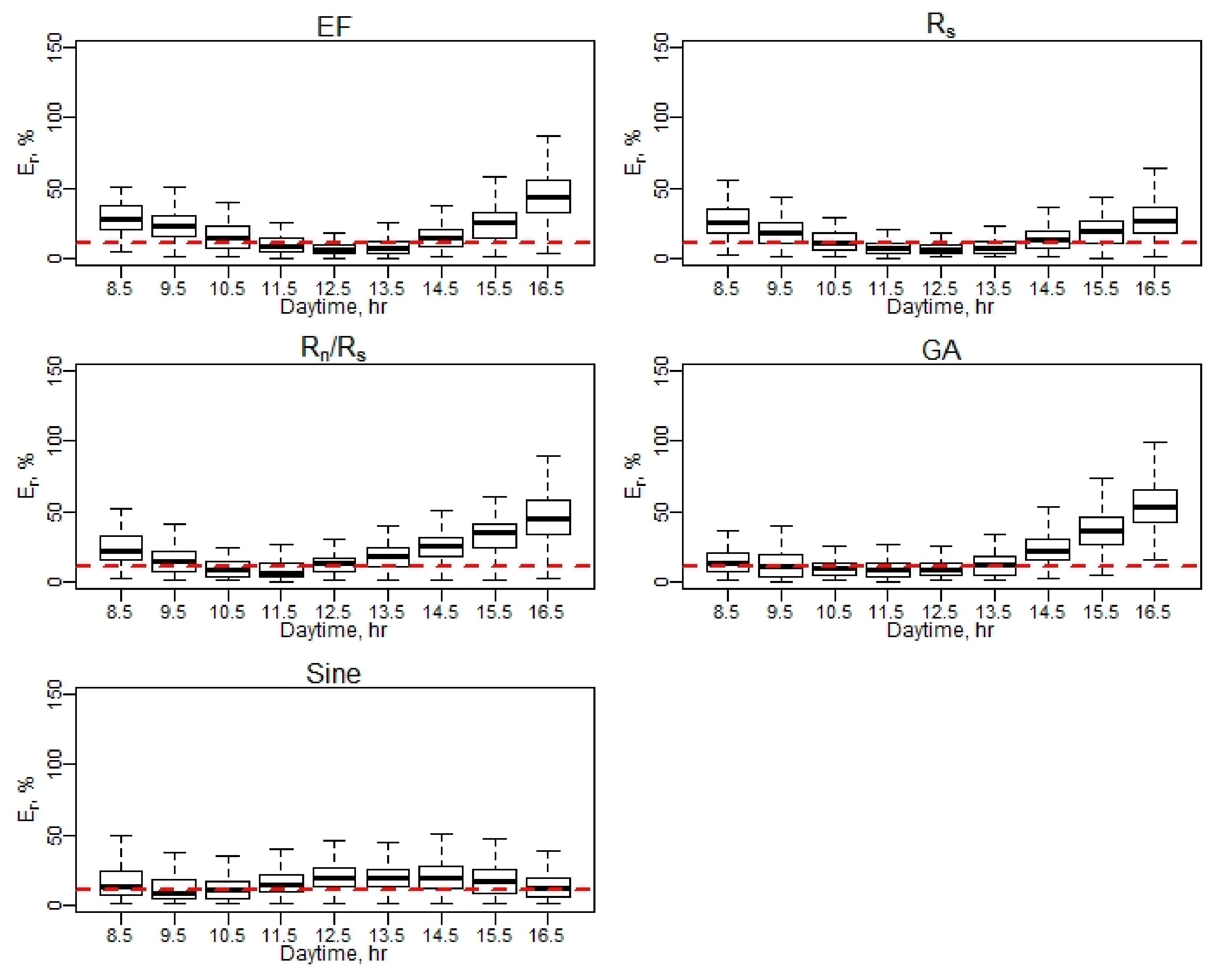
Appendix B.4. Relative Error (Er) at Hourly Scale for EC Measurements


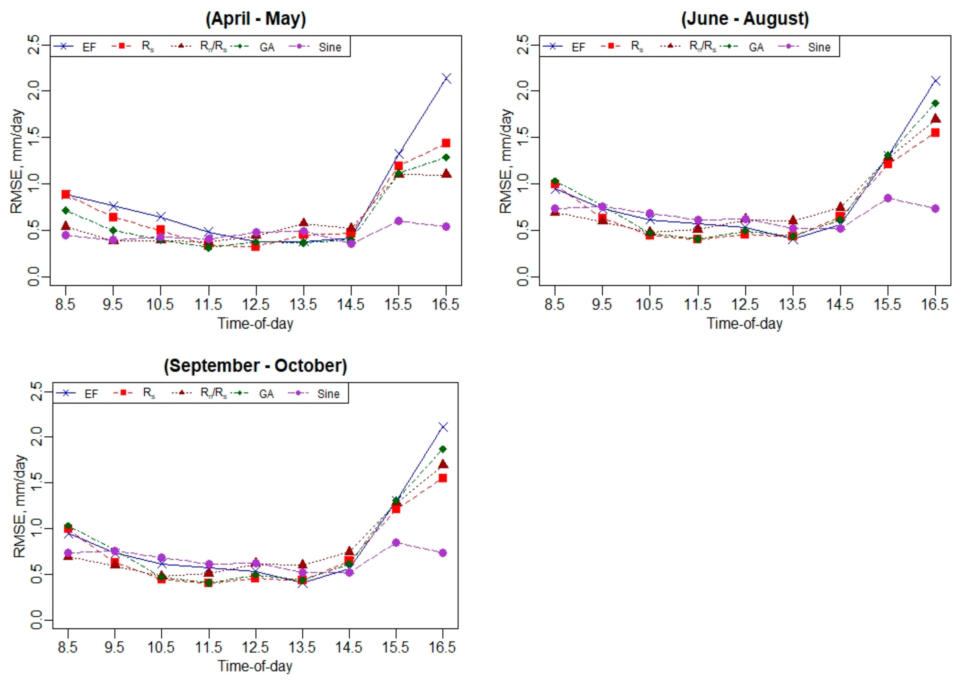
Appendix B.5. Daily RMSE Performance Using Hourly EC ET Values

Appendix C. Daily ET Analysis at Ripperdan 720 Vineyard, California
Appendix C.1. Diurnal Variation of Surface Energy Fluxes (Rn, H, LE, and G)

Appendix C.2. Hourly ET-to-Maximum Hourly ET Ratio (ETh/ETh(max)) Variation Using EC Measurements

Appendix C.3. Hourly ET-to-Daily ET Ratio (ETh/ETd) Variation Using EC Measurements

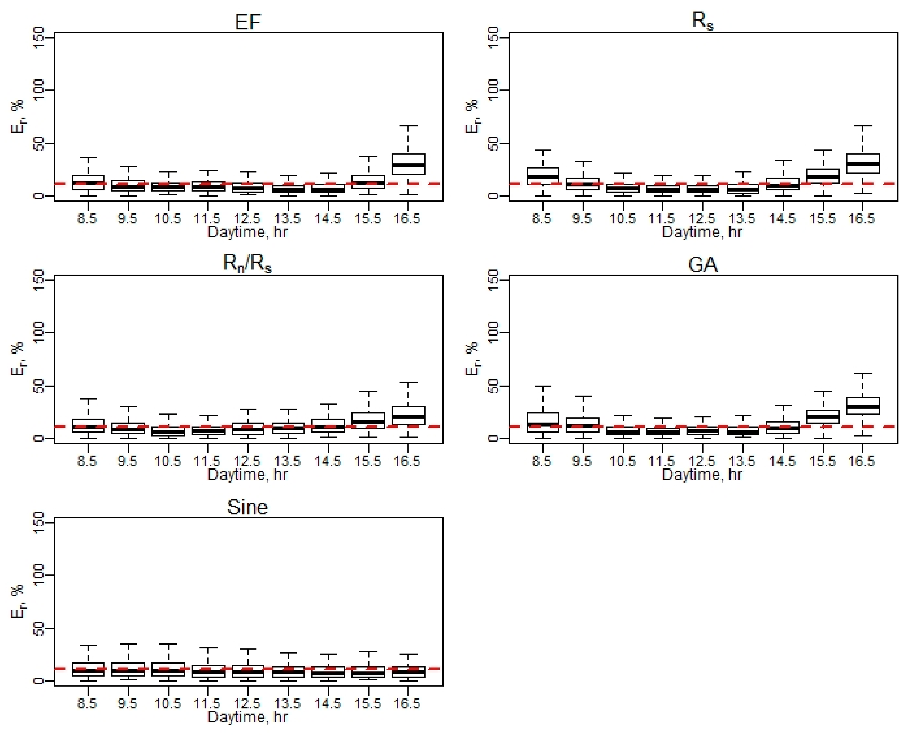
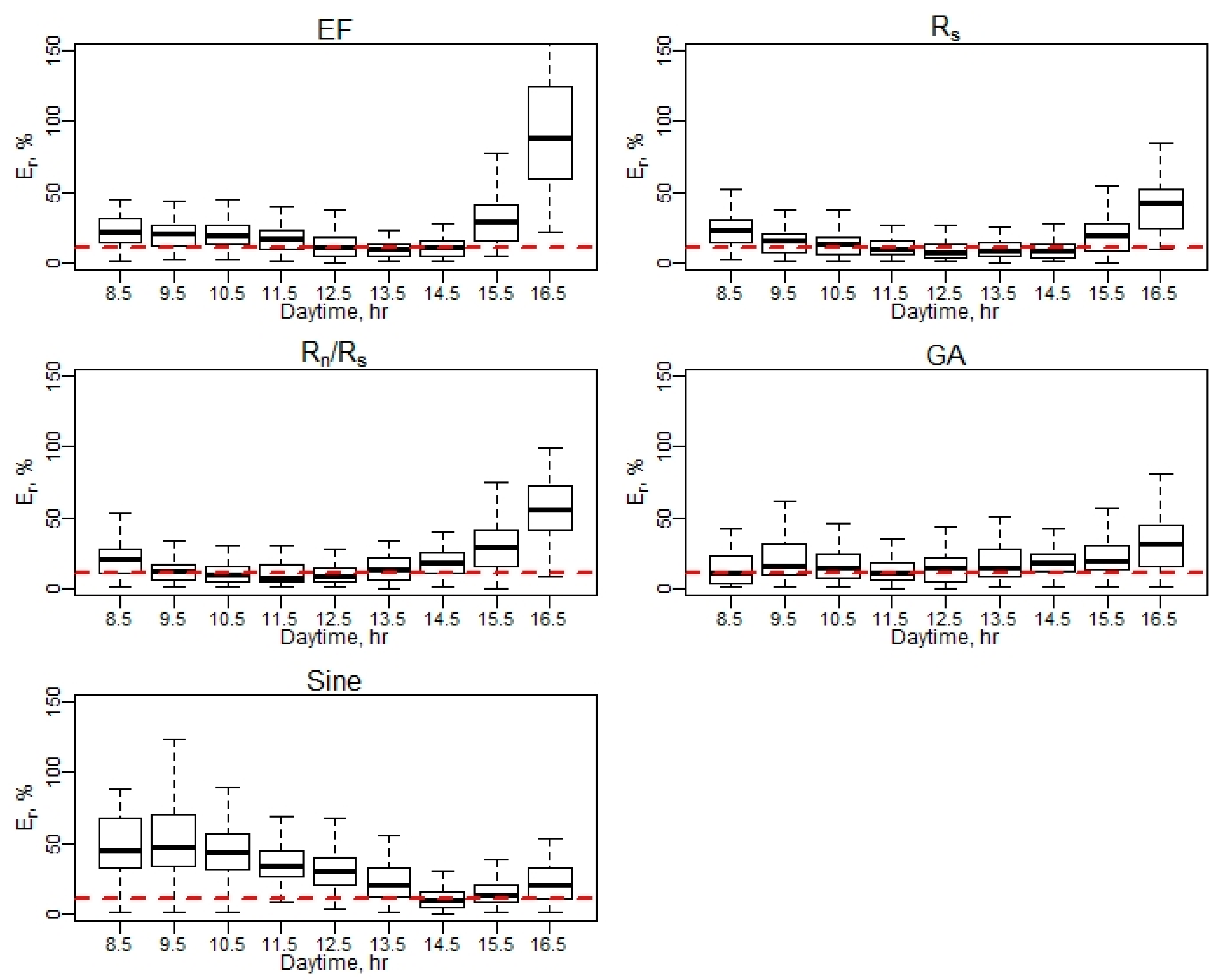
Appendix C.4. Relative Error (Er) at Hourly Scale for EC Measurements


Appendix C.5. Daily RMSE Performance Using Hourly EC ET Values

Appendix D. Daily ET Analysis at Barrelli Vineyard, California
Appendix D.1. Diurnal Variation of Surface Energy Fluxes (Rn, H, LE, and G)

Appendix D.2. Hourly ET-to-Maximum Hourly ET Ratio (ETh/ETh(max)) Variation Using EC Measurements

Appendix D.3. Hourly ET-to-Daily ET Ratio (ETh/ETd) Variation Using EC Measurements

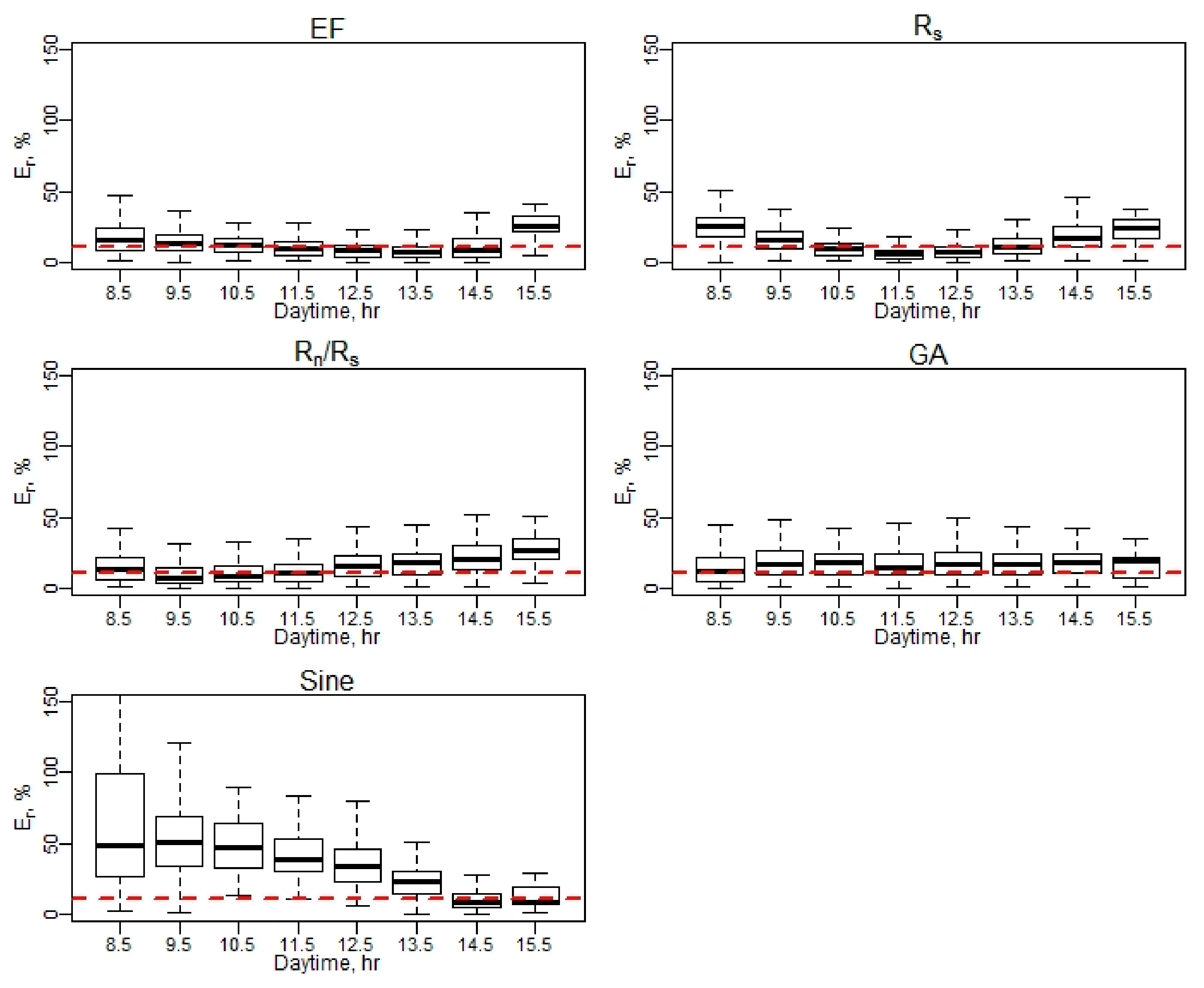
Appendix D.4. Relative Error (Er) at Hourly Scale for EC Measurements


Appendix D.5. Daily RMSE Performance Using Hourly EC ET Values

References
- Yang, H.; Yang, D.; Lei, Z.; Sun, F. New Analytical Derivation of the Mean Annual Water-Energy Balance Equation. Water Resour. Res. 2008, 44. [Google Scholar] [CrossRef]
- Housh, M.; Cai, X.; Ng, T.L.; McIsaac, G.F.; Ouyang, Y.; Khanna, M.; Sivapalan, M.; Jain, A.K.; Eckhoff, S.; Gasteyer, S.; et al. System of Systems Model for Analysis of Biofuel Development. J. Infrastruct. Syst. 2015, 21, 04014050. [Google Scholar] [CrossRef] [Green Version]
- Jiang, Y.; Jiang, X.; Tang, R.; Li, Z.-L.; Zhang, Y.; Huang, C.; Ru, C. Estimation of Daily Evapotranspiration Using Instantaneous Decoupling Coefficient from the MODIS and Field Data. IEEE J. Sel. Top. Appl. Earth Obs. Remote Sens. 2018, 11, 1832–1838. [Google Scholar] [CrossRef]
- Allen, R.G.; Tasumi, M.; Morse, A.; Trezza, R. A Landsat-Based Energy Balance and Evapotranspiration Model in Western US Water Rights Regulation and Planning. Irrig. Drain. Syst. 2005, 19, 251–268. [Google Scholar] [CrossRef]
- Anderson, M.C.; Kustas, W.P.; Norman, J.M.; Hain, C.R.; Mecikalski, J.R.; Schultz, L.; González-Dugo, M.P.; Cammalleri, C.; d’Urso, G.; Pimstein, A.; et al. Mapping Daily Evapotranspiration at Field to Continental Scales Using Geostationary and Polar Orbiting Satellite Imagery. Hydrol. Earth Syst. Sci. 2011, 15, 223–239. [Google Scholar] [CrossRef] [Green Version]
- Anderson, M.C.; Allen, R.G.; Morse, A.; Kustas, W.P. Use of Landsat Thermal Imagery in Monitoring Evapotranspiration and Managing Water Resources. Remote Sens. Environ. 2012, 122, 50–65. [Google Scholar] [CrossRef]
- Nassar, A.; Torres-Rua, A.; Kustas, W.; Nieto, H.; McKee, M.; Hipps, L.; Stevens, D.; Alfieri, J.; Prueger, J.; Alsina, M.M.; et al. Influence of Model Grid Size on the Estimation of Surface Fluxes Using the Two Source Energy Balance Model and sUAS Imagery in Vineyards. Remote Sens 2020, 12, 342. [Google Scholar] [CrossRef] [Green Version]
- Drexler, J.Z.; Snyder, R.L.; Spano, D.; Paw U, K.T. A Review of Models and Micrometeorological Methods Used to Estimate Wetland Evapotranspiration. Hydrol. Process. 2004, 18, 2071–2101. [Google Scholar] [CrossRef]
- Ortega-Farias, S.; Carrasco, M.; Olioso, A.; Acevedo, C.; Poblete, C. Latent Heat Flux over Cabernet Sauvignon Vineyard Using the Shuttleworth and Wallace Model. Irrig. Sci. 2006, 25, 161–170. [Google Scholar] [CrossRef]
- Parry, C.K.; Nieto, H.; Guillevic, P.; Agam, N.; Kustas, W.P.; Alfieri, J.; McKee, L.; McElrone, A.J. An Intercomparison of Radiation Partitioning Models in Vineyard Canopies. Irrig. Sci. 2019, 37, 239–252. [Google Scholar] [CrossRef]
- Nieto, H.; Kustas, W.P.; Alfieri, J.G.; Gao, F.; Hipps, L.E.; Los, S.; Prueger, J.H.; McKee, L.G.; Anderson, M.C. Impact of Different within-Canopy Wind Attenuation Formulations on Modelling Sensible Heat Flux Using TSEB. Irrig. Sci. 2019, 37, 315–331. [Google Scholar] [CrossRef]
- University of California Agriculture; the California Garden Web. Available online: http://cagardenweb.ucanr.edu (accessed on 25 December 2020).
- Mitcham, E.J.; Elkins, R.B. Pear Production and Handling Manual; University of California: Oakland, CA, USA, 2007; ISBN 9781879906655. [Google Scholar]
- Prueger, J.H.; Parry, C.K.; Kustas, W.P.; Alfieri, J.G.; Alsina, M.M.; Nieto, H.; Wilson, T.G.; Hipps, L.E.; Anderson, M.C.; Hatfield, J.L.; et al. Crop Water Stress Index of an Irrigated Vineyard in the Central Valley of California. Irrig. Sci. 2019, 37, 297–313. [Google Scholar] [CrossRef] [Green Version]
- USDA—National Agricultural Statistics Service—California. Available online: http://www.nass.usda.gov/ca (accessed on 25 December 2020).
- Alfieri, J.G.; Kustas, W.P.; Nieto, H.; Prueger, J.H.; Hipps, L.E.; McKee, L.G.; Gao, F.; Los, S. Influence of Wind Direction on the Surface Roughness of Vineyards. Irrig. Sci. 2019, 37, 359–373. [Google Scholar] [CrossRef]
- Nassar, A.; Torres-Rua, A.F.; Nieto, H.; Alfieri, J.G.; Hipps, L.E.; Prueger, J.H.; Alsina, M.M.; McKee, L.G.; White, W.; Kustas, W.P.; et al. Implications of Soil and Canopy Temperature Uncertainty in the Estimation of Surface Energy Fluxes Using TSEB2T and High-Resolution Imagery in Commercial Vineyards. In Proceedings of the SPIE, Online, 26 May 2020. [Google Scholar]
- Niu, H.; Zhao, T.; Wang, D.; Chen, Y. Evapotranspiration Estimation with UAVs in Agriculture: A Review. Preprints 2019. [Google Scholar] [CrossRef]
- Chávez, J.L.; Neale, C.M.U.; Prueger, J.H.; Kustas, W.P. Daily Evapotranspiration Estimates from Extrapolating Instantaneous Airborne Remote Sensing ET Values. Irrig. Sci. 2008, 27, 67–81. [Google Scholar] [CrossRef]
- Cammalleri, C.; Anderson, M.C.; Gao, F.; Hain, C.R.; Kustas, W.P. A Data Fusion Approach for Mapping Daily Evapotranspiration at Field Scale. Water Resour. Res. 2013, 49, 4672–4686. [Google Scholar] [CrossRef]
- Cammalleri, C.; Anderson, M.C.; Gao, F.; Hain, C.R.; Kustas, W.P. Mapping Daily Evapotranspiration at Field Scales over Rainfed and Irrigated Agricultural Areas Using Remote Sensing Data Fusion. Agric. For. Meteorol. 2014, 186, 1–11. [Google Scholar] [CrossRef] [Green Version]
- Knipper, K.R.; Kustas, W.P.; Anderson, M.C.; Alsina, M.M.; Hain, C.R.; Alfieri, J.G.; Prueger, J.H.; Gao, F.; McKee, L.G.; Sanchez, L.A. Using High-Spatiotemporal Thermal Satellite ET Retrievals for Operational Water Use and Stress Monitoring in a California Vineyard. Remote Sens. 2019, 11, 2124. [Google Scholar] [CrossRef] [Green Version]
- Tsouros, D.C.; Bibi, S.; Sarigiannidis, P.G. A Review on UAV-Based Applications for Precision Agriculture. Information 2019, 10, 349. [Google Scholar] [CrossRef] [Green Version]
- Nielsen, H.H.M. Evapotranspiration from UAV Images: A New Scale of Measurements; Department of Geosciences and Natural Resource Management, Faculty of Science, University of Copenhagen: Copenhagen, Denmark, 2016. [Google Scholar]
- Nassar, A.; Torres-Rue, A.F.; McKee, M.; Kustas, W.P.; Coopmans, C.; Nieto, H.; Hipps, L. Assessment of UAV Flight Times for Estimation of Daily High Resolution Evapotranspiration in Complex Agricultural Canopy Environments; Universities Council in Water Resources (UCOWR): Snowbird, UT, USA, 2019. [Google Scholar]
- Zhang, C.; Long, D.; Zhang, Y.; Anderson, M.C.; Kustas, W.P.; Yang, Y. A Decadal (2008–2017) Daily Evapotranspiration Data Set of 1 Km Spatial Resolution and Spatial Completeness across the North China Plain Using TSEB and Data Fusion. Remote Sens. Environ. 2021, 262, 112519. [Google Scholar] [CrossRef]
- Allen, G.; Morton, C.; Kamble, B.; Kilic, A.; Huntington, J.; Thau, D.; Gorelick, N.; Erickson, T.; Moore, R.; Trezza, R.; et al. 2015 EEFlux: A Landsat-Based Evapotranspiration Mapping Tool on the Google Earth Engine. In Proceedings of the 2015 ASABE/IA Irrigation Symposium: Emerging Technologies for Sustainable Irrigation—A Tribute to the Career of Terry Howell, Sr. Conference Proceedings, Long Beach, CA, USA, 10–12 November 2015. [Google Scholar]
- Colaizzi, P.D.; Evett, S.R.; Howell, T.A.; Tolk, J.A. Comparison of Five Models to Scale Daily Evapotranspiration from One-Time-of-Day Measurements. Trans. ASABE 2006, 49, 1409–1417. [Google Scholar] [CrossRef]
- Cammalleri, C.; Anderson, M.C.; Kustas, W.P. Upscaling of Evapotranspiration Fluxes from Instantaneous to Daytime Scales for Thermal Remote Sensing Applications. Hydrol. Earth Syst. Sci. 2014, 18, 1885–1894. [Google Scholar] [CrossRef] [Green Version]
- Jackson, R.D.; Hatfield, J.L.; Reginato, R.J.; Idso, S.B.; Pinter, P.J. Estimation of Daily Evapotranspiration from One Time-of-Day Measurements. Agric. Water Manag. 1983, 7, 351–362. [Google Scholar] [CrossRef]
- Crago, R.D. Conservation and Variability of the Evaporative Fraction during the Daytime. J. Hydrol. 1996, 180, 173–194. [Google Scholar] [CrossRef]
- Crago, R.D. Comparison of the Evaporative Fraction and the Priestley-Taylor α for Parameterizing Daytime Evaporation. Water Resour. Res. 1996, 32, 1403–1409. [Google Scholar] [CrossRef]
- Delogu, E.; Boulet, G.; Olioso, A.; Coudert, B.; Chirouze, J.; Ceschia, E.; Le Dantec, V.; Marloie, O.; Chehbouni, G.; Lagouarde, -P.J. Reconstruction of Temporal Variations of Evapotranspiration Using Instantaneous Estimates at the Time of Satellite Overpass. Hydrol. Earth Syst. Sci. 2012, 16, 2995–3010. [Google Scholar] [CrossRef] [Green Version]
- Suleiman, A.; Crago, R. Hourly and Daytime Evapotranspiration from Grassland Using Radiometric Surface Temperatures. Agron. J. 2004, 96, 384. [Google Scholar] [CrossRef]
- Shuttleworth, W.J.; Gurney, R.J.; Hsu, A.Y.; Ormsby, J.P. FIFE: The Variation in Energy Partition at Surface Flux Sites. IAHS Publ. 1989, 186, 523–534. [Google Scholar]
- Hoedjes, J.C.B.; Chehbouni, A.; Jacob, F.; Ezzahar, J.; Boulet, G. Deriving Daily Evapotranspiration from Remotely Sensed Instantaneous Evaporative Fraction over Olive Orchard in Semi-Arid Morocco. J. Hydrol. 2008, 354, 53–64. [Google Scholar] [CrossRef] [Green Version]
- Li, S.; Kang, S.; Li, F.; Zhang, L.; Zhang, B. Vineyard Evaporative Fraction Based on Eddy Covariance in an Arid Desert Region of Northwest China. Agric. Water Manag. 2008, 95, 937–948. [Google Scholar] [CrossRef]
- Zhang, L.; Lemeur, R. Evaluation of Daily Evapotranspiration Estimates from Instantaneous Measurements. Agric. For. Meteorol. 1995, 74, 139–154. [Google Scholar] [CrossRef]
- Gentine, P.; Entekhabi, D.; Chehbouni, A.; Boulet, G.; Duchemin, B. Analysis of Evaporative Fraction Diurnal Behaviour. Agric. For. Meteorol. 2007, 143, 13–29. [Google Scholar] [CrossRef] [Green Version]
- Van Niel, T.; McVicar, T.; Roderick, M.; Dijk, A.; Beringer, J.; Hutley, L.; Gorsel, E. Upscaling Latent Heat Flux for Thermal Remote Sensing Studies: Comparison of Alternative Approaches and Correction of Bias. J. Hydrol. 2012, 468–469, 35–46. [Google Scholar] [CrossRef]
- Wandera, L.; Mallick, K.; Kiely, G.; Roupsard, O.; Peichl, M.; Magliulo, V. Upscaling Instantaneous to Daily Evapotranspiration Using Modelled Daily Shortwave Radiation for Remote Sensing Applications: An Artificial Neural Network Approach. Hydrol. Earth Syst. Sci. 2017, 21, 197–215. [Google Scholar] [CrossRef] [Green Version]
- French, A.N.; Fitzgerald, G.; Hunsaker, D.; Barnes, E.; Clarke, T.; Lesch, S.; Roth, R.; Pinter, P. Estimating Spatially Distributed Cotton Water Use from Thermal Infrared Aerial Imagery. Impacts Glob. Clim. Chang. 2005. [Google Scholar] [CrossRef]
- Liu, S.; Su, H.; Zhang, R.; Tian, J.; Chen, S.; Wang, W.; Yang, L.; Liang, H. Based on the Gaussian Fitting Method to Derive Daily Evapotranspiration from Remotely Sensed Instantaneous Evapotranspiration. Adv. Meteorol. 2019, 2019, 1–13. [Google Scholar] [CrossRef]
- Norman, J.M.; Kustas, W.P.; Humes, K.S. Source Approach for Estimating Soil and Vegetation Energy Fluxes in Observations of Directional Radiometric Surface Temperature. Agric. For. Meteorol. 1995, 77, 263–293. [Google Scholar] [CrossRef]
- Norman, J.M.; Kustas, W.P.; Prueger, J.H.; Diak, G.R. Surface Flux Estimation Using Radiometric Temperature: A Dual-Temperature-Difference Method to Minimize Measurement Errors. Water Resour. Res. 2000, 36, 2263–2274. [Google Scholar] [CrossRef] [Green Version]
- Kustas, W.P.; Alfieri, J.G.; Anderson, M.C.; Colaizzi, P.D.; Prueger, J.H.; Evett, S.R.; Neale, C.M.U.; French, A.N.; Hipps, L.E.; Chávez, J.L.; et al. Evaluating the Two-Source Energy Balance Model Using Local Thermal and Surface Flux Observations in a Strongly Advective Irrigated Agricultural Area. Adv. Water Resour. 2012, 50, 120–133. [Google Scholar] [CrossRef] [Green Version]
- Gao, F.; Kustas, W.; Anderson, M. A Data Mining Approach for Sharpening Thermal Satellite Imagery over Land. Remote Sens. 2012, 4, 3287–3319. [Google Scholar] [CrossRef] [Green Version]
- Kustas, W.P.; Norman, J.M. A Two-Source Approach for Estimating Turbulent Fluxes Using Multiple Angle Thermal Infrared Observations. Water Resour. Res. 1997, 33, 1495–1508. [Google Scholar] [CrossRef]
- Nieto, H.; Kustas, W.P.; Torres-Rúa, A.; Alfieri, J.G.; Gao, F.; Anderson, M.C.; White, W.A.; Song, L.; Del Mar Alsina, M.; Prueger, J.H.; et al. Evaluation of TSEB Turbulent Fluxes Using Different Methods for the Retrieval of Soil and Canopy Component Temperatures from UAV Thermal and Multispectral Imagery. Irrig. Sci. 2019, 37, 389–406. [Google Scholar] [CrossRef] [PubMed] [Green Version]
- Xia, T.; Kustas, W.P.; Anderson, M.C.; Alfieri, J.G.; Gao, F.; McKee, L.; Prueger, J.H.; Geli, H.M.E.; Neale, C.M.U.; Sanchez, L.; et al. Mapping Evapotranspiration with High-Resolution Aircraft Imagery over Vineyards Using One- and Two-Source Modeling Schemes. Hydrol. Earth Syst. Sci. 2016, 20, 1523–1545. [Google Scholar] [CrossRef] [Green Version]
- Brutsaert, W. Aspects of Bulk Atmospheric Boundary Layer Similarity under Free-Convective Conditions. Rev. Geophys. 1999, 37, 439–451. [Google Scholar] [CrossRef]
- Kustas, W.P.; Nieto, H.; Morillas, L.; Anderson, M.C.; Alfieri, J.G.; Hipps, L.E.; Villagarcía, L.; Domingo, F.; Garcia, M. Revisiting the Paper “Using Radiometric Surface Temperature for Surface Energy Flux Estimation in Mediterranean Drylands from a Two-Source Perspective”. Remote Sens. Environ. 2016, 184, 645–653. [Google Scholar] [CrossRef] [Green Version]
- Kondo, J.; Ishida, S. Sensible Heat Flux from the Earth’s Surface under Natural Convective Conditions. J. Atmos. Sci. 1997, 54, 498–509. [Google Scholar] [CrossRef]
- Kustas, W.P.; Anderson, M.C.; Alfieri, J.G.; Knipper, K.; Torres-Rua, A.; Parry, C.K.; Nieto, H.; Agam, N.; White, W.A.; Gao, F.; et al. The Grape Remote Sensing Atmospheric Profile and Evapotranspiration Experiment. Bull. Am. Meteorol. Soc. 2018, 99, 1791–1812. [Google Scholar] [CrossRef] [PubMed] [Green Version]
- Utah State University AggieAir. Available online: https://uwrl.usu.edu/aggieair/index (accessed on 25 December 2020).
- Torres-Rua, A. Vicarious Calibration of sUAS Microbolometer Temperature Imagery for Estimation of Radiometric Land Surface Temperature. Sensors 2017, 17, 1499. [Google Scholar] [CrossRef] [Green Version]
- Torres-Rua, A.F.; Ticlavilca, A.M.; Aboutalebi, M.; Nieto, H.; Alsina, M.M.; White, A.; Prueger, J.H.; Alfieri, J.G.; Hipps, L.E.; McKee, L.G.; et al. Estimation of Evapotranspiration and Energy Fluxes Using a Deep-Learning-Based High-Resolution Emissivity Model and the Two-Source Energy Balance Model with sUAS Information. In Proceedings of the SPIE, Online, 14 May 2020. [Google Scholar]
- Hassan-Esfahani, L.; Ebtehaj, A.M.; Torres-Rua, A.; McKee, M. Spatial Scale Gap Filling Using an Unmanned Aerial System: A Statistical Downscaling Method for Applications in Precision Agriculture. Sensors 2017, 17, 2106. [Google Scholar] [CrossRef] [Green Version]
- Kljun, N.; Calanca, P.; Rotach, M.W.; Schmid, H.P. A simple two-dimensional parameterisation for Flux Footprint Prediction (FFP). Geosci. Model Dev. 2015, 8, 3695–3713. [Google Scholar] [CrossRef] [Green Version]
- Sun, H.; Yang, Y.; Wu, R.; Gui, D.; Xue, J.; Liu, Y.; Yan, D. Improving Estimation of Cropland Evapotranspiration by the Bayesian Model Averaging Method with Surface Energy Balance Models. Atmosphere 2019, 10, 188. [Google Scholar] [CrossRef] [Green Version]
- Li, S.; Tong, L.; Li, F.; Zhang, L.; Zhang, B.; Kang, S. Variability in Energy Partitioning and Resistance Parameters for a Vineyard in Northwest China. Agric. Water Manag. 2009, 96, 955–962. [Google Scholar] [CrossRef]
- Brutsaert, W.; Chen, D. Diurnal Variation of Surface Fluxes During Thorough Drying (or Severe Drought) of Natural Prairie. Water Resour. Res. 1996, 32, 2013–2019. [Google Scholar] [CrossRef]
- Sugita, M.; Brutsaert, W. Daily Evaporation over a Region from Lower Boundary Layer Profiles Measured with Radiosondes. Water Resour. Res. 1991, 27, 747–752. [Google Scholar] [CrossRef]
- Shapland, T.M.; Snyder, R.L.; Smart, D.R.; Williams, L.E. Estimation of Actual Evapotranspiration in Winegrape Vineyards Located on Hillside Terrain Using Surface Renewal Analysis. Irrig. Sci. 2012, 30, 471–484. [Google Scholar] [CrossRef]
- Tolk, J.A.; Howell, T.A.; Evett, S.R. Nighttime Evapotranspiration from Alfalfa and Cotton in a Semiarid Climate. Agron. J. 2006, 98, 730–736. [Google Scholar] [CrossRef] [Green Version]
- Knipper, K.R.; Kustas, W.P.; Anderson, M.C.; Nieto, H.; Alfieri, J.G.; Prueger, J.H.; Hain, C.R.; Gao, F.; McKee, L.G.; Mar Alsina, M.; et al. Using High-Spatiotemporal Thermal Satellite ET Retrievals to Monitor Water Use over California Vineyards of Different Climate, Vine Variety and Trellis Design. Agric. Water Manag. 2020, 241, 106361. [Google Scholar] [CrossRef]
- Semmens, K.A.; Anderson, M.C.; Kustas, W.P.; Gao, F.; Alfieri, J.G.; McKee, L.; Prueger, J.H.; Hain, C.R.; Cammalleri, C.; Yang, Y.; et al. Monitoring Daily Evapotranspiration over Two California Vineyards Using Landsat 8 in a Multi-Sensor Data Fusion Approach. Remote Sens. Environ. 2016, 185, 155–170. [Google Scholar] [CrossRef] [Green Version]
- Neale, C.M.U.; Geli, H.M.E.; Kustas, W.P.; Alfieri, J.G.; Gowda, P.H.; Evett, S.R.; Prueger, J.H.; Hipps, L.E.; Dulaney, W.P.; Chávez, J.L.; et al. Soil Water Content Estimation Using a Remote Sensing Based Hybrid Evapotranspiration Modeling Approach. Adv. Water Resour. 2012, 50, 152–161. [Google Scholar] [CrossRef]
- Kustas, W.P.; Prueger, J.H.; Hatfield, J.L.; Ramalingam, K.; Hipps, L.E. Variability in Soil Heat Flux from a Mesquite Dune Site. Agric. For. Meteorol. 2000, 103, 249–264. [Google Scholar] [CrossRef]


| Site | Date | Time PST 1 | Spectral Bands 2 | Satellite’s Overpass |
|---|---|---|---|---|
| Sierra Loma | 9 August 2014 | 1041 | RGBNIR 3 | Landsat |
| Sierra Loma | 2 June 2015 | 1043 | RGBNIR | Landsat |
| Sierra Loma | 2 June 2015 | 1407 | RGBRE | NA |
| Sierra Loma | 11 July 2015 | 1035 | RGBNIR | Landsat |
| Sierra Loma | 11 July 2015 | 1414 | RGB | NA |
| Sierra Loma | 2 May 2016 | 1205 | REDNIR | NA |
| Sierra Loma | 2 May 2016 | 1504 | REDNIR | NA |
| Sierra Loma | 3 May 2016 | 1248 | REDNIR | NA |
| Barrelli | 8 August 2017 | 1052 | RGBNIR | Landsat |
| Barrelli | 9 August 2017 | 1043 | RGBNIR | Landsat |
| Ripperdan 760 | 24 July 2017 | 1035 | RGBNIR | Sentinel 3 |
| Ripperdan 760 | 25 July 2017 | 1035 | RGBNIR | Landsat |
| Ripperdan 760 | 25 July 2017 | 1357 | RGBNIR | NA |
| Ripperdan 760 | 25 July 2017 | 1634 | RGBNIR | NA |
| Ripperdan 760 | 26 July 2017 | 1426 | RGBNIR | NA |
| Ripperdan 760 | 5 August 2018 | 1044 | RGBNIR | Landsat |
| Ripperdan 760 | 5 August 2018 | 1234 | RGBNIR | NA |
| Ripperdan 720 | 5 August 2018 | 1044 | RGBNIR | Landsat |
| Ripperdan 720 | 5 August 2018 | 1234 | RGBNIR | NA |
| Vineyard | Number of EC Towers | Elevation (agl) | EC Tower Name | Latitude 1 | Longitude 1 | Period of Data (Years) |
|---|---|---|---|---|---|---|
| Sierra Loma | 2 | 5 | 1 | 38°16′49.76″ | −121°7′3.35″ | 5 |
| 2 | 38°17′21.62″ | −121°7′3.95″ | 5 | |||
| Ripperdan 760 | 1 | 3.5 | 1 | 36°50′20.52″ | −120°12′36.60″ | 2 |
| Ripperdan 720 | 4 | 3.5 | 1 | 36°50′57.27″ | −120°10′26.50″ | 1 |
| 2 | 36°50′51.40″ | −120°10′26.69″ | 1 | |||
| 3 | 36°50′57.26″ | −120°10′33.83″ | 1 | |||
| 4 | 36°50′51.39″ | −120°10′34.02″ | 1 | |||
| Barrelli | 1 | 3.5 | 1 | 38°45′4.91″ | −122°58′28.77″ | 2 |
| Vine Stage | Method | 1030–1330 | 1430–1630 | ||||||||
|---|---|---|---|---|---|---|---|---|---|---|---|
| RMSE (mm/day) | MAE (mm/day) | MAPE (%) | NSE | R2 | RMSE (mm/day) | MAE (mm/day) | MAPE (%) | NSE | R2 | ||
| Bloom (April–May) | EF | 0.36 | 0.28 | 10 | 0.83 | 0.85 | 1.02 | 0.71 | 29 | −0.75 | 0.55 |
| Rs | 0.35 | 0.26 | 10 | 0.85 | 0.87 | 0.64 | 0.50 | 19 | 0.31 | 0.81 | |
| Rn/Rs | 1.33 | 0.82 | 29 | −1.25 | 0.15 | 1.49 | 1.13 | 43 | −2.68 | 0.06 | |
| GA | 0.38 | 0.30 | 11 | 0.81 | 0.87 | 0.87 | 0.72 | 28 | −0.26 | 0.77 | |
| Sine | 0.56 | 0.47 | 18 | 0.60 | 0.86 | 0.50 | 0.39 | 15 | 0.59 | 0.82 | |
| Veraison (June–August) | EF | 0.47 | 0.32 | 9 | 0.81 | 0.85 | 0.97 | 0.70 | 21 | 0.07 | 0.63 |
| Rs | 0.38 | 0.29 | 8 | 0.88 | 0.89 | 0.70 | 0.57 | 17 | 0.51 | 0.83 | |
| Rn/Rs | 1.67 | 0.90 | 22 | −1.41 | 0.17 | 1.78 | 1.26 | 35 | −2.14 | 0.08 | |
| GA | 0.43 | 0.33 | 9 | 0.84 | 0.87 | 1.12 | 0.96 | 29 | −0.23 | 0.72 | |
| Sine | 0.65 | 0.53 | 14 | 0.64 | 0.86 | 0.63 | 0.51 | 15 | 0.61 | 0.84 | |
| Post-harvest (September–October) | EF | 0.28 | 0.21 | 13 | 0.93 | 0.95 | 2.53 | 0.68 | 55 | −6.76 | 0.10 |
| Rs | 0.25 | 0.19 | 11 | 0.94 | 0.95 | 0.49 | 0.37 | 23 | 0.71 | 0.92 | |
| Rn/Rs | 0.47 | 0.31 | 16 | 0.80 | 0.88 | 1.02 | 0.63 | 42 | −0.27 | 0.62 | |
| GA | 0.40 | 0.31 | 17 | 0.86 | 0.95 | 0.53 | 0.41 | 25 | 0.66 | 0.93 | |
| Sine | 0.77 | 0.64 | 36 | 0.45 | 0.92 | 0.31 | 0.24 | 16 | 0.88 | 0.92 | |
| All stages (Season) | EF | 0.41 | 0.29 | 10 | 0.91 | 0.92 | 1.50 | 0.70 | 31 | −0.57 | 0.43 |
| Rs | 0.34 | 0.26 | 9 | 0.93 | 0.94 | 0.64 | 0.51 | 19 | 0.71 | 0.90 | |
| Rn/Rs | 1.38 | 0.73 | 22 | −0.08 | 0.37 | 1.56 | 1.08 | 38 | −0.71 | 0.23 | |
| GA | 0.41 | 0.32 | 12 | 0.90 | 0.93 | 0.95 | 0.77 | 28 | 0.37 | 0.86 | |
| Sine | 0.67 | 0.55 | 21 | 0.75 | 0.91 | 0.54 | 0.42 | 15 | 0.80 | 0.91 | |
| Site | Fluxes | RMSE (W/m2) | MAE (W/m2) | MAPE (%) | NSE | R2 |
|---|---|---|---|---|---|---|
| Sierra Loma | Rn | 43 | 36 | 7 | 0.85 | 0.90 |
| H | 37 | 31 | 27 | 0.61 | 0.70 | |
| LE | 51 | 38 | 15 | 0.40 | 0.40 | |
| G | 55 | 50 | 96 | 0.08 | 0.30 | |
| Ripperdan 760 | Rn | 36 | 31 | 5 | 0.91 | 0.96 |
| H | 37 | 27 | 19 | 0.86 | 0.96 | |
| LE | 58 | 50 | 19 | 0.28 | 0.52 | |
| G | 27 | 20 | 66 | 0.11 | 0.21 | |
| Ripperdan 720 | Rn | 35 | 28 | 4 | 0.17 | 0.53 |
| H | 54 | 42 | 20 | 0.73 | 0.90 | |
| LE | 52 | 49 | 15 | 0.81 | 0.94 | |
| G | 14 | 14 | 23 | −0.01 | 0.31 | |
| Barrelli | Rn | 26 | 23 | 4 | 0.58 | NA 1 |
| H | 62 | 46 | 22 | −0.92 | NA | |
| LE | 40 | 38 | 26 | 0.11 | NA | |
| G | 71 | 71 | 196 | 0.01 | NA | |
| All vineyards | Rn | 39 | 32 | 6 | 0.90 | 0.90 |
| H | 43 | 34 | 23 | 0.80 | 0.80 | |
| LE | 52 | 43 | 17 | 0.70 | 0.80 | |
| G | 45 | 36 | 78 | 0.20 | 0.40 |
| Sites | Method | 1030–1330 | 1430–1630 | ||||||||
|---|---|---|---|---|---|---|---|---|---|---|---|
| RMSE (mm/day) | MAE (mm/day) | MAPE (%) | NSE | R2 | RMSE (mm/day) | MAE (mm/day) | MAPE (%) | NSE | R2 | ||
| Sierra Loma | EF | 0.44 | 0.32 | 10 | 0.57 | 0.63 | 1.02 | 0.89 | 27 | −7 | 0.00 |
| Rs | 0.38 | 0.32 | 10 | 0.67 | 0.78 | 0.95 | 0.72 | 22 | −6 | 0.00 | |
| Rn/Rs | 0.95 | 0.77 | 23 | −0.96 | 0.67 | 1.30 | 1.05 | 31 | −12.08 | 0.05 | |
| GA | 0.44 | 0.39 | 13 | 0.58 | 0.82 | 1.02 | 0.79 | 24 | −7.02 | 0.01 | |
| Sine | 0.80 | 0.63 | 18 | −0.41 | 0.79 | 1.01 | 0.76 | 24 | −6.93 | 0.00 | |
| Ripperdan 760 | EF | 0.39 | 0.34 | 8 | 0.24 | 0.93 | 1.85 | 1.5 | 36 | −33.52 | 0.55 |
| Rs | 0.62 | 0.55 | 13 | −0.82 | 0.45 | 1.65 | 1.34 | 33 | −26.54 | 0.69 | |
| Rn/Rs | 0.73 | 0.62 | 14 | −3.43 | 0.70 | 2.12 | 1.77 | 43 | −44.70 | 0.67 | |
| GA | 0.63 | 0.61 | 14 | −2.26 | 0.55 | 2.39 | 1.99 | 48 | −56.82 | 0.28 | |
| Sine | 1.60 | 1.34 | 31 | −20.18 | 0.19 | 1.83 | 1.63 | 38 | −33 | 0.04 | |
| Ripperdan 720 | EF | 0.49 | 0.44 | 11 | 0.80 | 0.92 | No flights | ||||
| Rs | 0.44 | 0.36 | 9 | 0.85 | 0.93 | ||||||
| Rn/Rs | 0.83 | 0.73 | 16 | 0.44 | 0.92 | ||||||
| GA | 0.59 | 0.47 | 11 | 0.72 | 0.91 | ||||||
| Sine | 1.68 | 1.47 | 31 | −1.26 | 0.94 | ||||||
| Barrelli | EF | 0.41 | 0.41 | 19 | NA | NA 1 | |||||
| Rs | 0.19 | 0.19 | 9 | NA | NA | ||||||
| Rn/Rs | 0.78 | 0.78 | 36 | NA | NA | ||||||
| GA | 0.67 | 0.67 | 31 | NA | NA | ||||||
| Sine | 0.86 | 0.86 | 40 | NA | NA | ||||||
| All vineyards | EF | 0.45 | 0.37 | 10 | 0.81 | 0.82 | 1.35 | 1.1 | 30 | −14.29 | 0.11 |
| Rs | 0.45 | 0.37 | 10 | 0.80 | 0.88 | 1.23 | 0.93 | 25 | −11.65 | 0.19 | |
| Rn/Rs | 0.87 | 0.73 | 20 | 0.29 | 0.82 | 1.62 | 1.29 | 35 | −21.06 | 0.22 | |
| GA | 0.54 | 0.47 | 13 | 0.71 | 0.87 | 1.61 | 1.19 | 32 | −20.72 | 0.25 | |
| Sine | 1.32 | 1.05 | 26 | −0.68 | 0.87 | 1.34 | 1.05 | 28 | −14.10 | 0.37 | |
Publisher’s Note: MDPI stays neutral with regard to jurisdictional claims in published maps and institutional affiliations. |
© 2021 by the authors. Licensee MDPI, Basel, Switzerland. This article is an open access article distributed under the terms and conditions of the Creative Commons Attribution (CC BY) license (https://creativecommons.org/licenses/by/4.0/).
Share and Cite
Nassar, A.; Torres-Rua, A.; Kustas, W.; Alfieri, J.; Hipps, L.; Prueger, J.; Nieto, H.; Alsina, M.M.; White, W.; McKee, L.; et al. Assessing Daily Evapotranspiration Methodologies from One-Time-of-Day sUAS and EC Information in the GRAPEX Project. Remote Sens. 2021, 13, 2887. https://doi.org/10.3390/rs13152887
Nassar A, Torres-Rua A, Kustas W, Alfieri J, Hipps L, Prueger J, Nieto H, Alsina MM, White W, McKee L, et al. Assessing Daily Evapotranspiration Methodologies from One-Time-of-Day sUAS and EC Information in the GRAPEX Project. Remote Sensing. 2021; 13(15):2887. https://doi.org/10.3390/rs13152887
Chicago/Turabian StyleNassar, Ayman, Alfonso Torres-Rua, William Kustas, Joseph Alfieri, Lawrence Hipps, John Prueger, Héctor Nieto, Maria Mar Alsina, William White, Lynn McKee, and et al. 2021. "Assessing Daily Evapotranspiration Methodologies from One-Time-of-Day sUAS and EC Information in the GRAPEX Project" Remote Sensing 13, no. 15: 2887. https://doi.org/10.3390/rs13152887