
Using Remote Sensing to Estimate Scales of Spatial Heterogeneity to Analyze Evapotranspiration Modeling in a Natural Ecosystem

 , , , ,
Abstract
:1. Introduction
2. Methodology
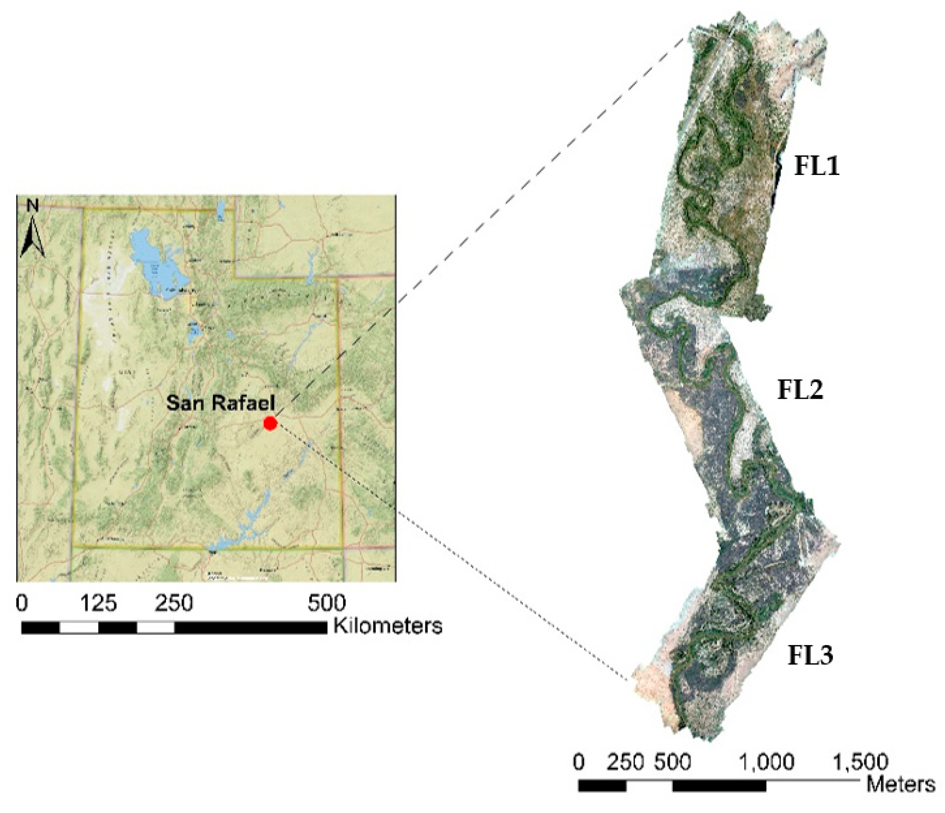
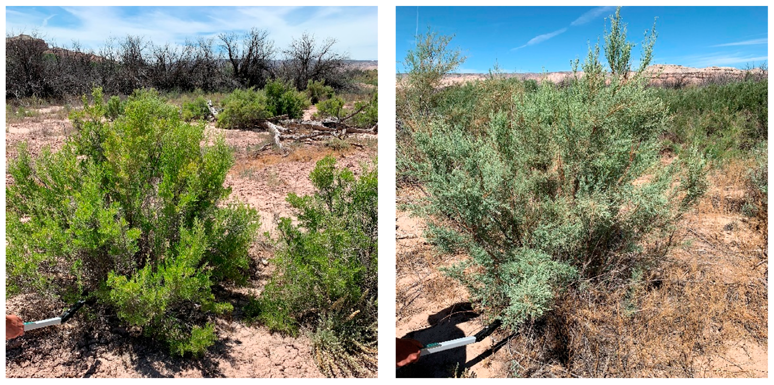
2.1. Site Description
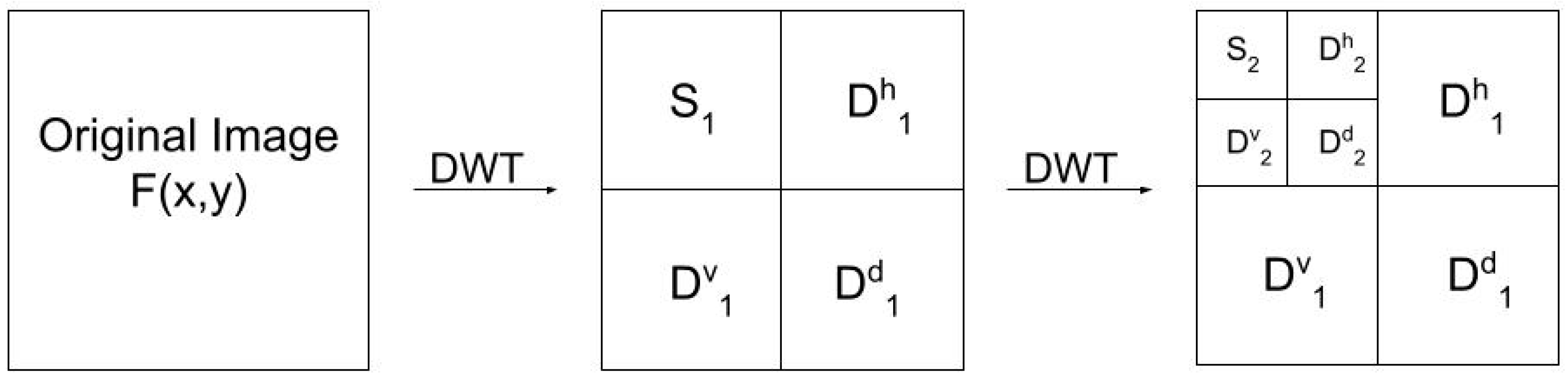
2.2. Characterizing the Spatial Heterogeneity Using Wavelet Analysis
2.3. Image Classification
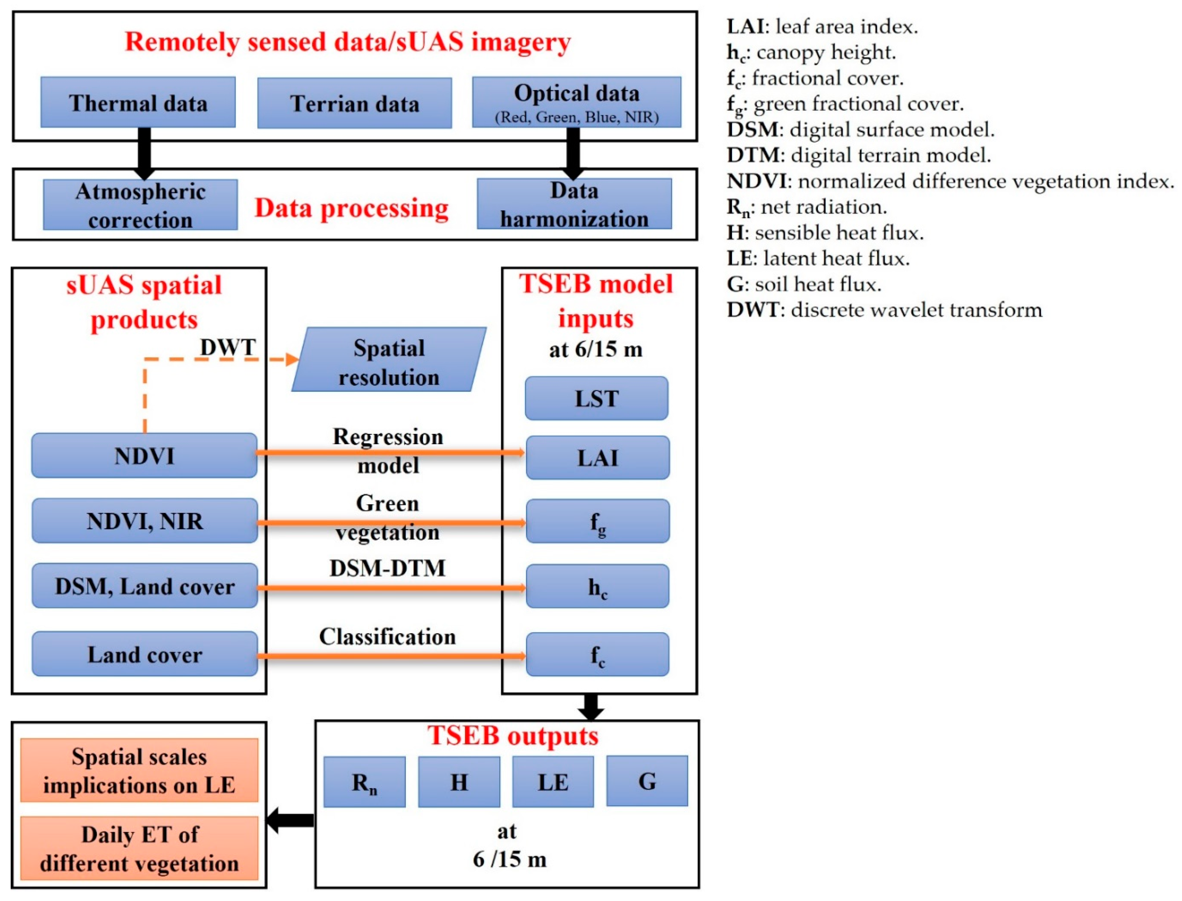
2.4. ET Estimation Using the Two-Source Energy Balance (TSEB) Model
2.4.1. Model Overview
2.4.2. Retrieving the Biophysical TSEB Inputs
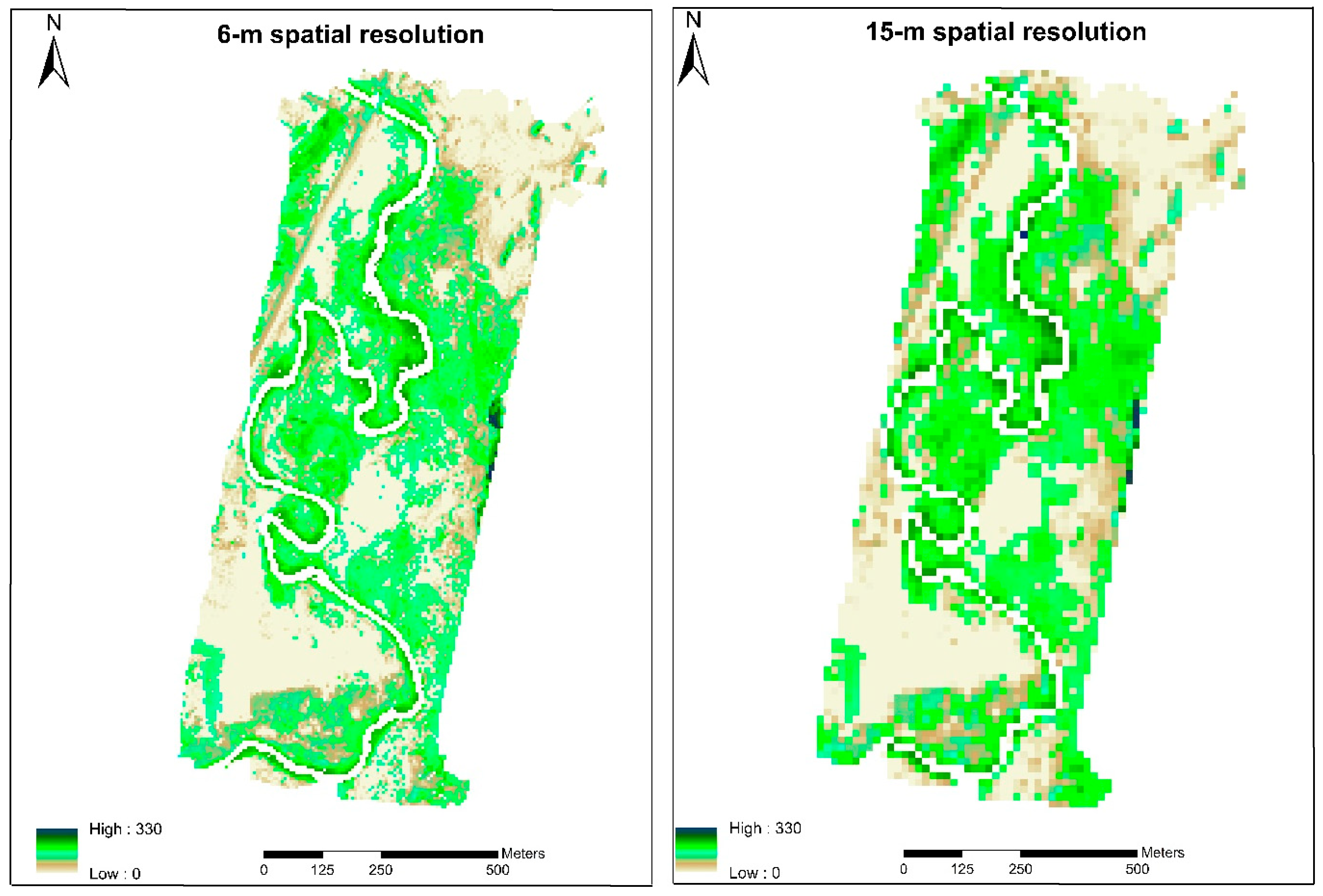
- (a)
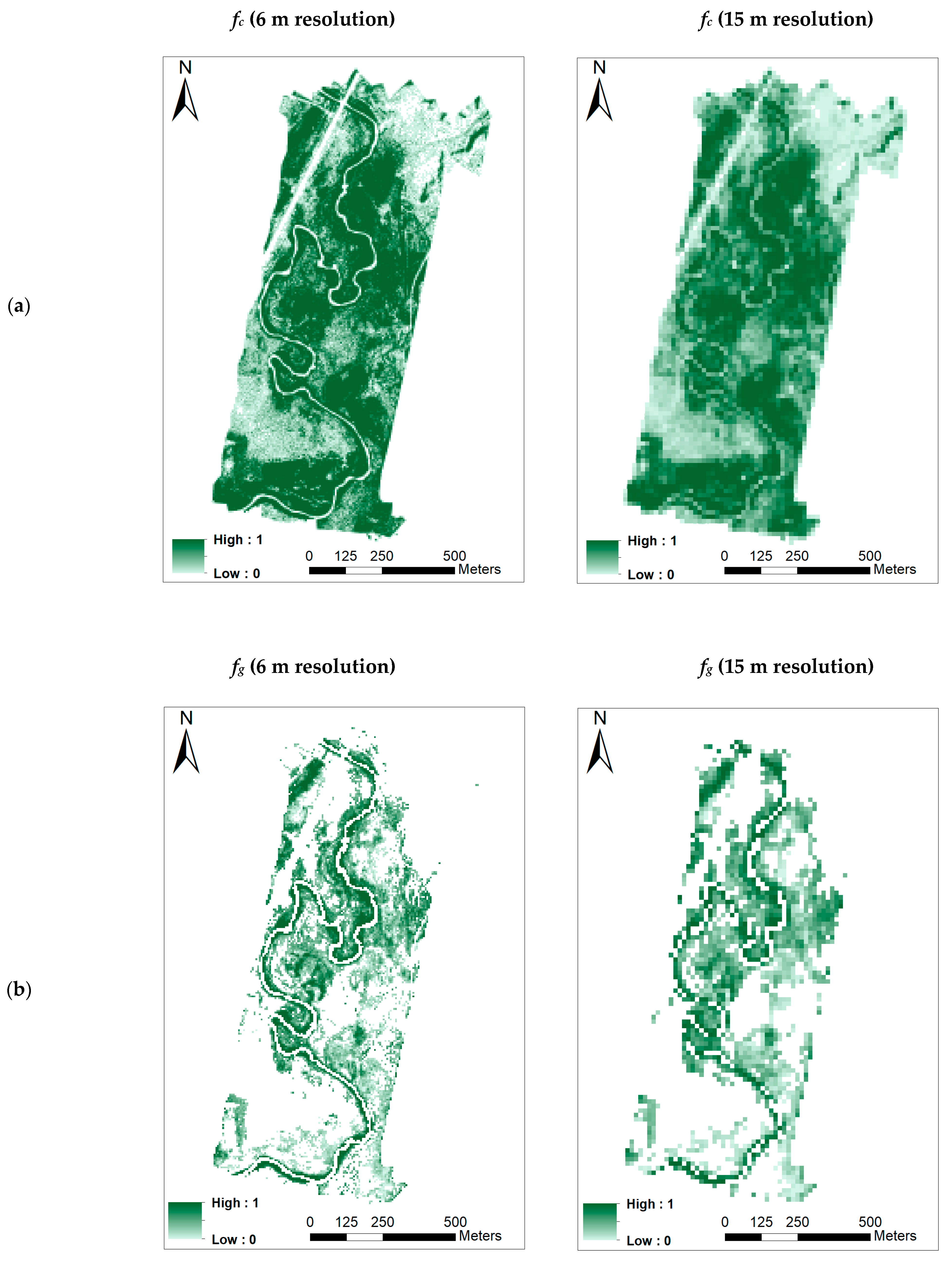
- Fractional cover (fc)
- (b)
- Green ground cover (fg)
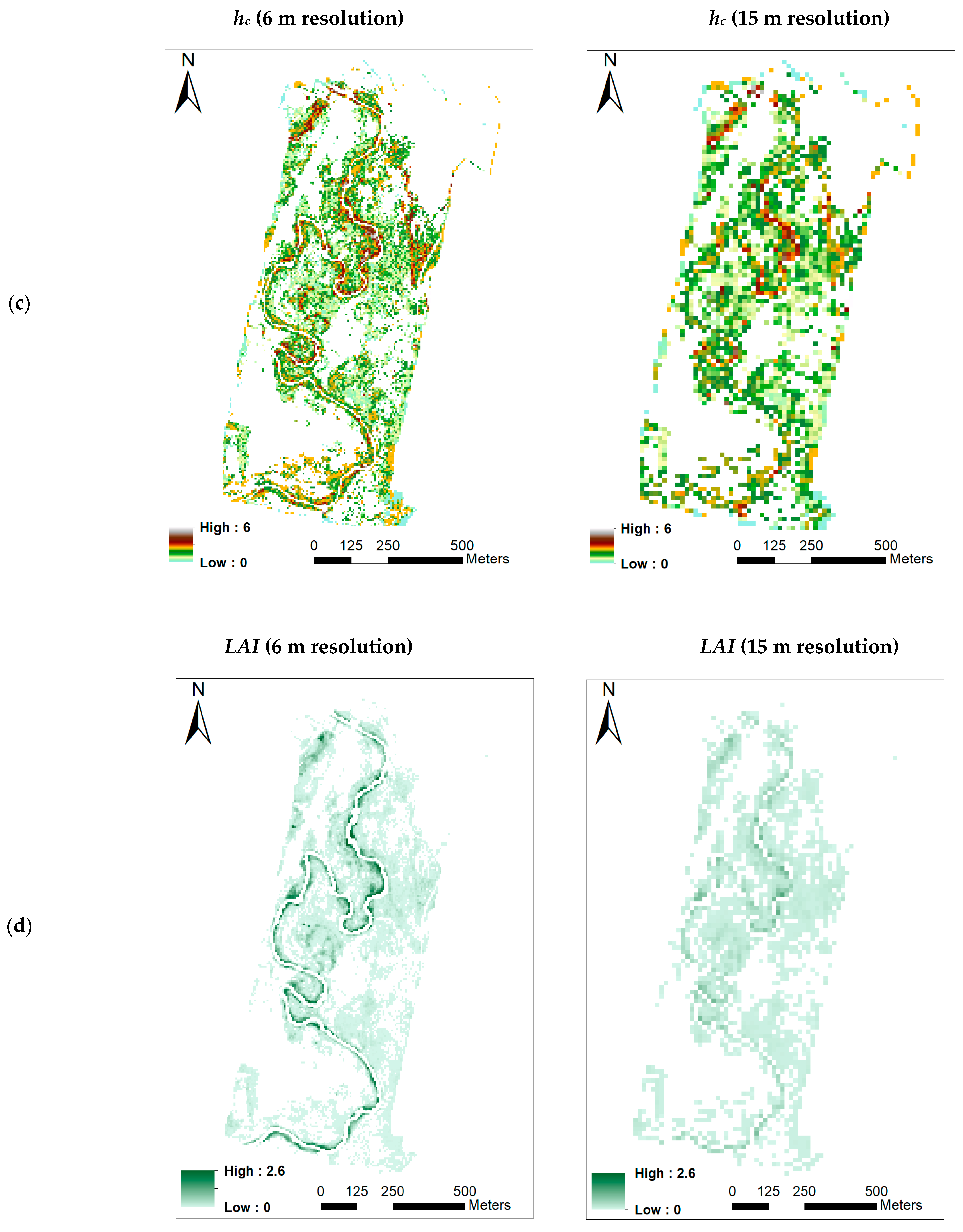
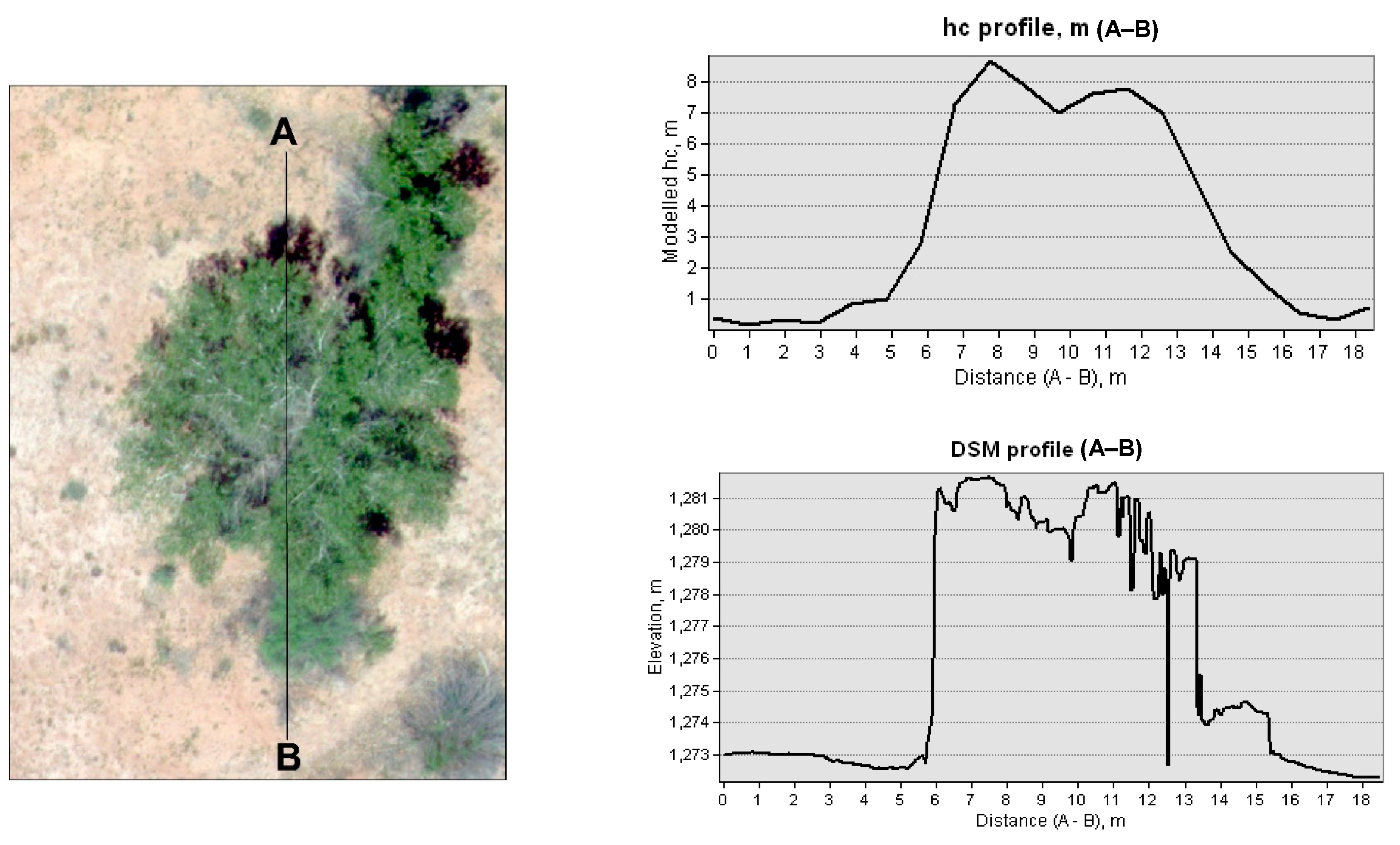
- (c)
- Canopy height (hc)
- (d)
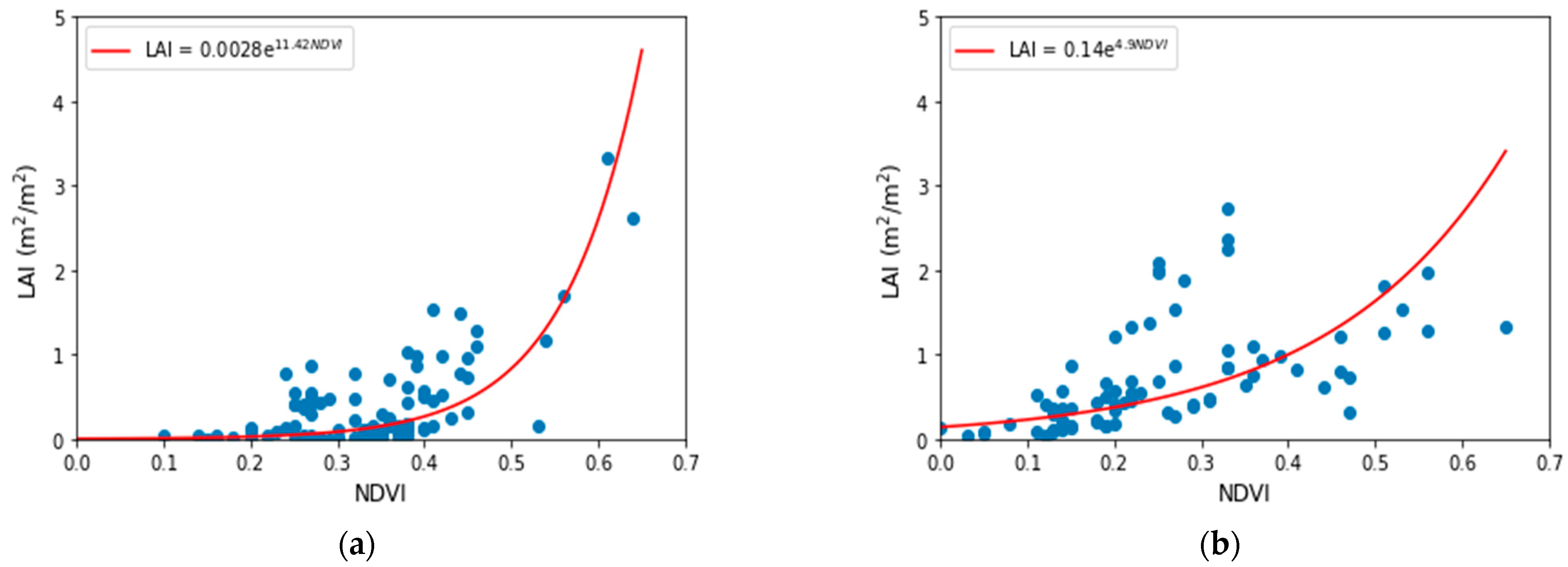
- Leaf Area Index (LAI)
2.5. Daily ET Estimation
3. Results and Discussion
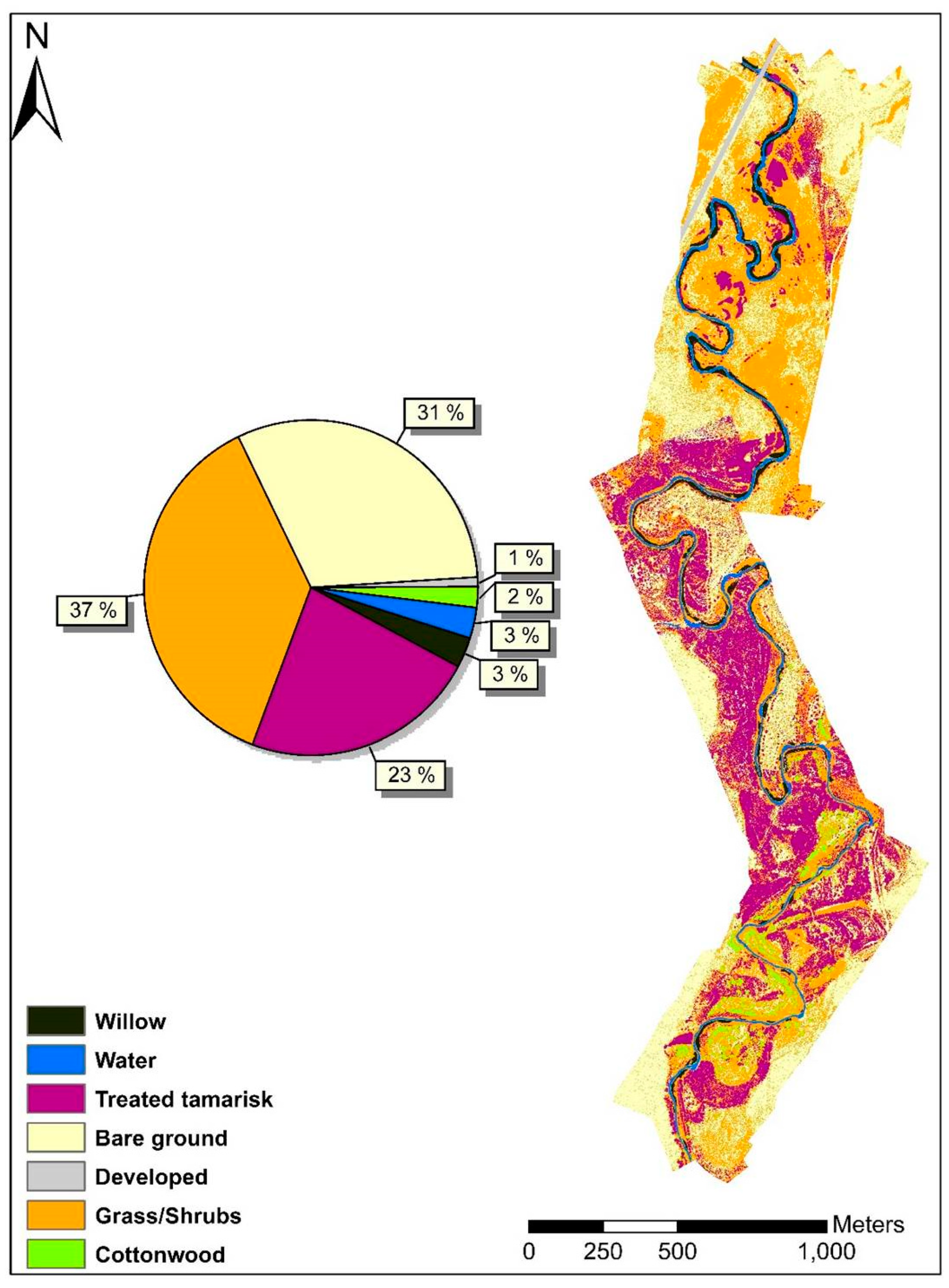
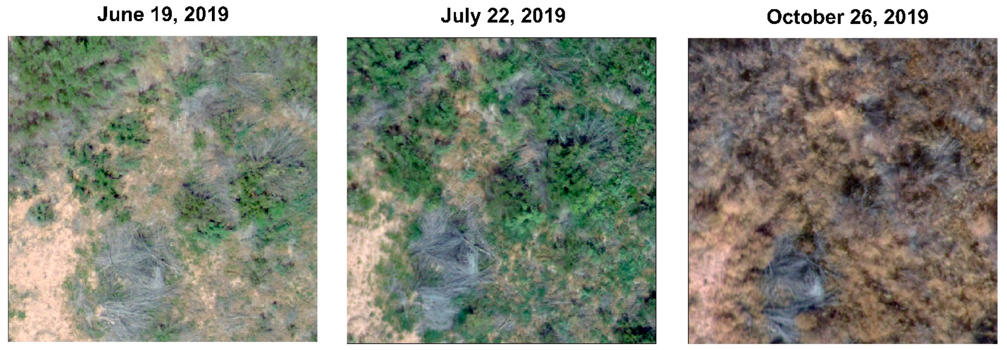
3.1. Land Cover/Land Use Classification
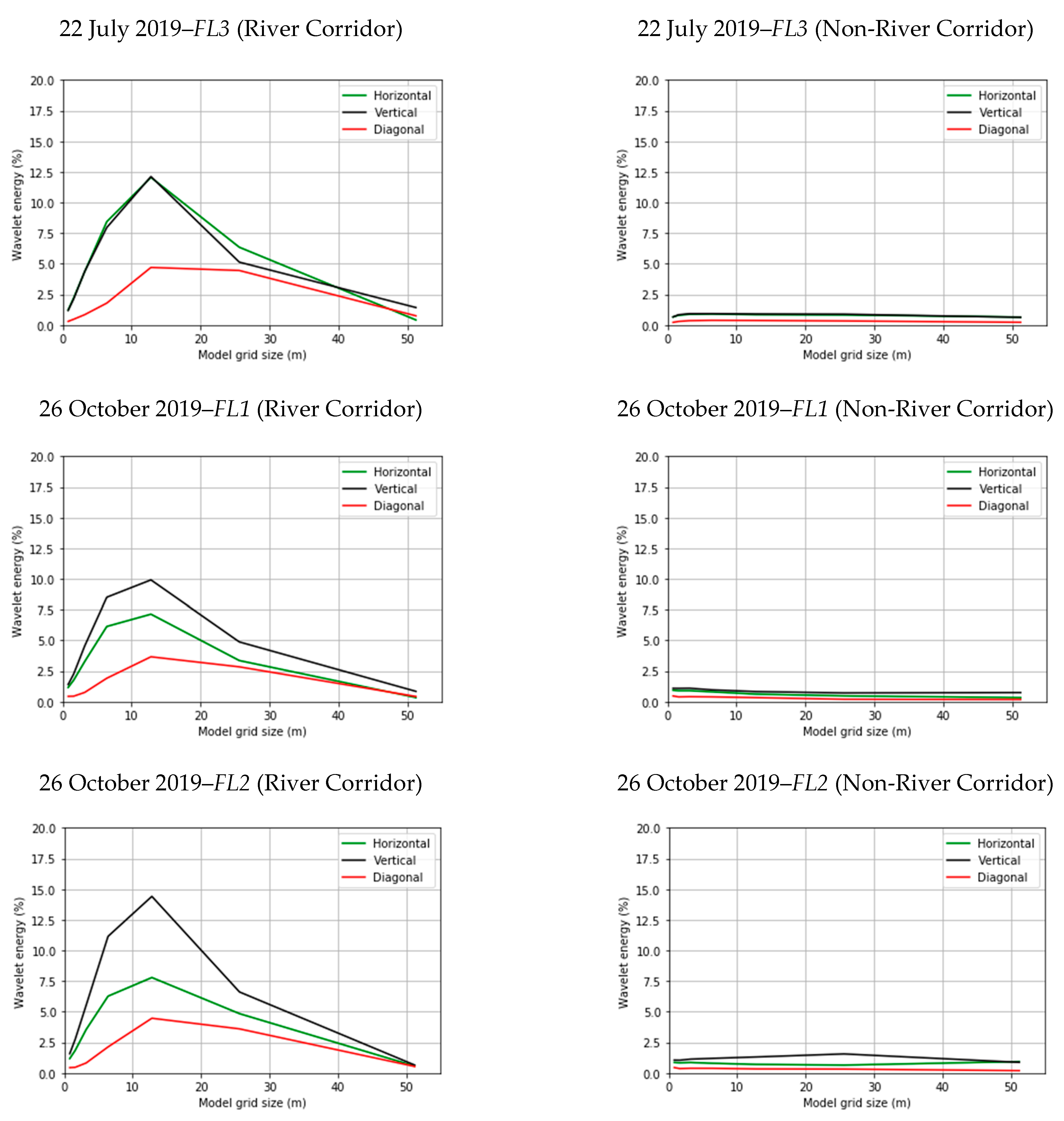
3.2. Spatial Heterogeneity Using Wavelet Analysis
3.3. Retrieving the Biophysical Parameters
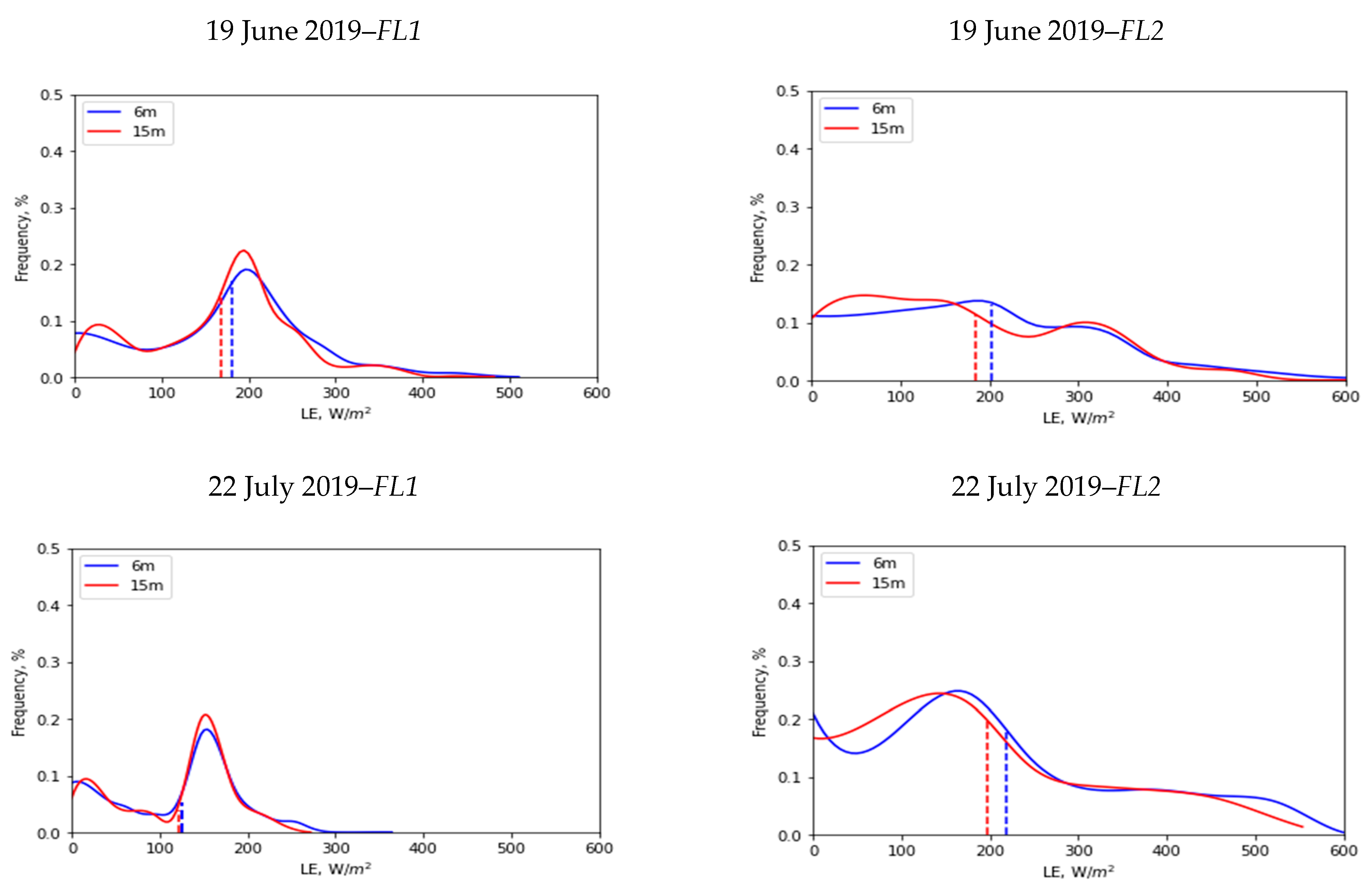
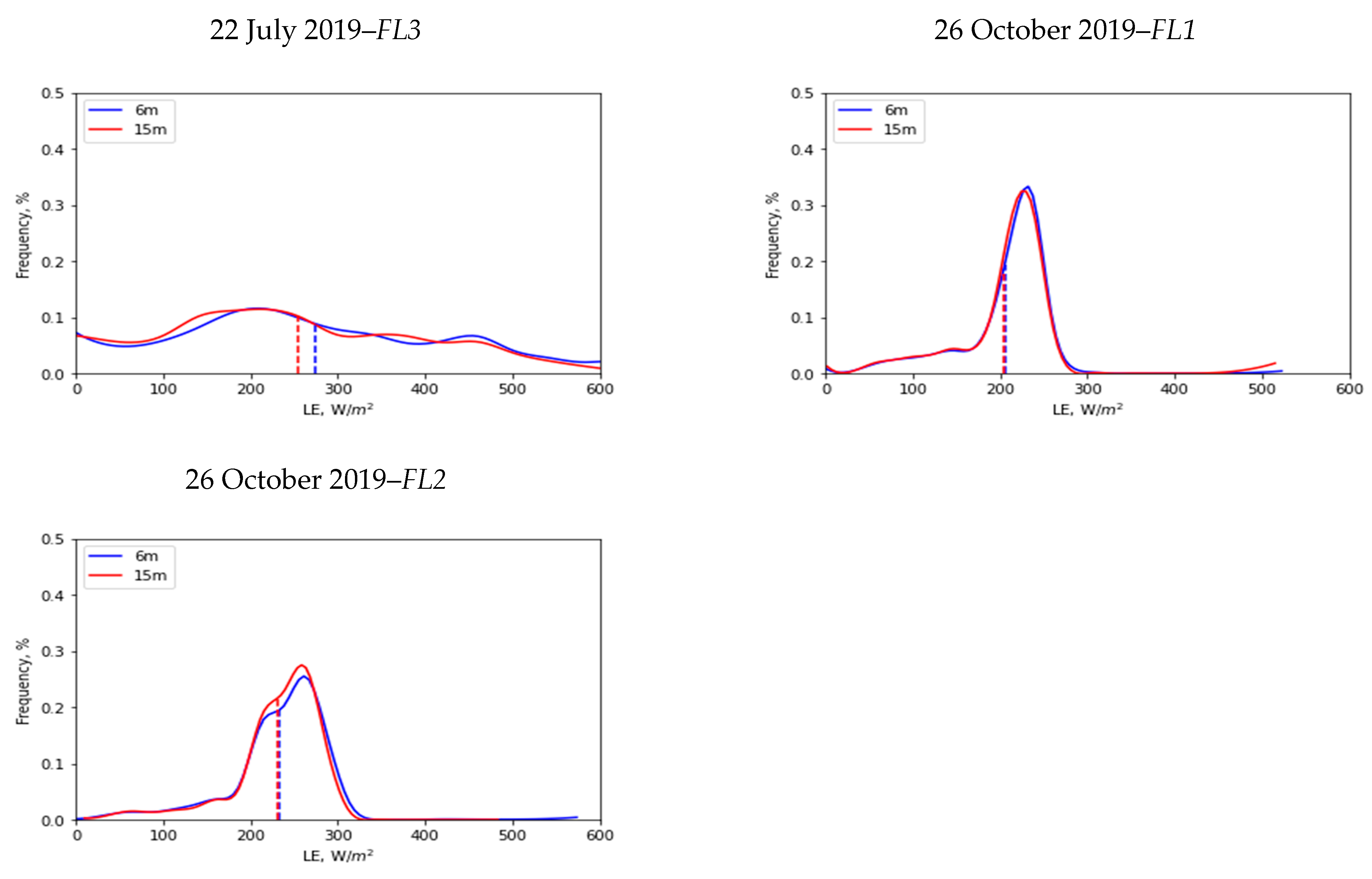
3.4. Spatial Scale Implications on LE
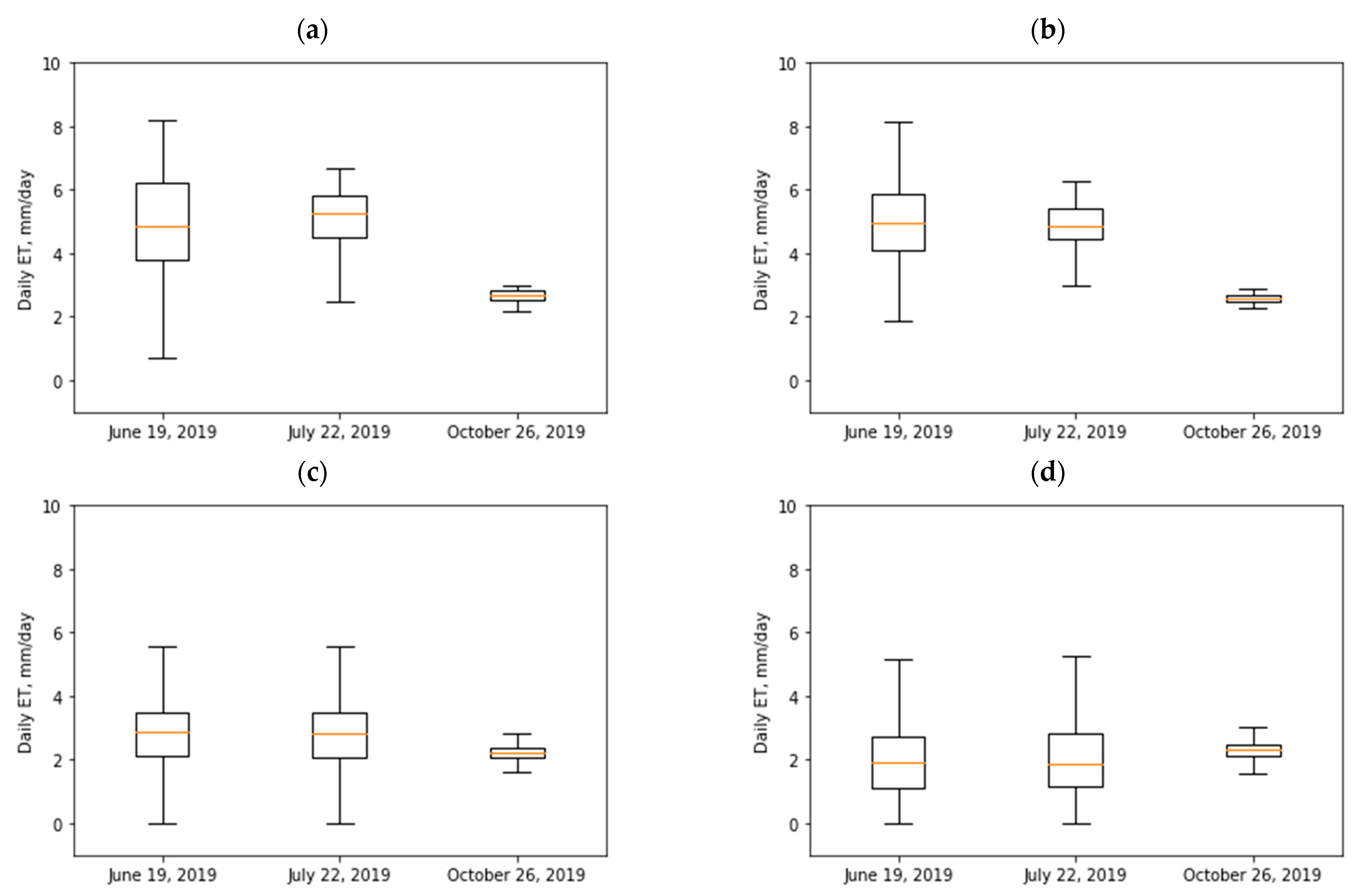
3.5. Daily ET Calculation for Vegetation Types
4. Conclusions
Author Contributions
Funding
Conflicts of Interest
References
- Glenn, E.P.; Huete, A.R.; Nagler, P.L.; Hirschboeck, K.K.; Brown, P. Integrating Remote Sensing and Ground Methods to Estimate Evapotranspiration. Crit. Rev. Plant Sci. 2007, 26, 139–168. [Google Scholar] [CrossRef]
- González-Dugo, M.P.; Chen, X.; Andreu, A.; Carpintero, E.; Gómez-Giraldez, P.J.; Carrara, A.; Su, Z. Long-Term Water Stress and Drought Monitoring of Mediterranean Oak Savanna Vegetation Using Thermal Remote Sensing. Hydrol. Earth Syst. Sci. 2021, 25, 755–768. [Google Scholar] [CrossRef]
- Nassar, A.; Torres-Rua, A.; Kustas, W.; Nieto, H.; McKee, M.; Hipps, L.; Stevens, D.; Alfieri, J.; Prueger, J.; Alsina, M.M.; et al. Influence of Model Grid Size on the Estimation of Surface Fluxes Using the Two Source Energy Balance Model and sUAS Imagery in Vineyards. Remote Sens. 2020, 12, 342. [Google Scholar] [CrossRef] [PubMed] [Green Version]
- Saadi, S.; Boulet, G.; Bahir, M.; Brut, A.; Delogu, É.; Fanise, P.; Mougenot, B.; Simonneaux, V.; Chabaane, Z.L. Assessment of Actual Evapotranspiration over a Semiarid Heterogeneous Land Surface by Means of Coupled Low-Resolution Remote Sensing Data with an Energy Balance Model: Comparison to Extra-Large Aperture Scintillometer Measurements. Hydrol. Earth Syst. Sci. 2018, 22, 2187–2209. [Google Scholar] [CrossRef] [Green Version]
- Giorgi, F.; Avissar, R. Representation of Heterogeneity Effects in Earth System Modeling: Experience from Land Surface Modeling. Rev. Geophys. 1997, 35, 413–437. [Google Scholar] [CrossRef]
- Bonan, G.B.; Doney, S.C. Climate, Ecosystems, and Planetary Futures: The Challenge to Predict Life in Earth System Models. Science 2018, 359, eaam8328. [Google Scholar] [CrossRef] [Green Version]
- Krinner, G.; Viovy, N.; de Noblet-Ducoudré, N.; Ogée, J.; Polcher, J.; Friedlingstein, P.; Ciais, P.; Sitch, S.; Colin Prentice, I. A Dynamic Global Vegetation Model for Studies of the Coupled Atmosphere-Biosphere System. Glob. Biogeochem. Cycles 2005, 19. [Google Scholar] [CrossRef]
- Richardson, A.D.; Keenan, T.F.; Migliavacca, M.; Ryu, Y.; Sonnentag, O.; Toomey, M. Climate Change, Phenology, and Phenological Control of Vegetation Feedbacks to the Climate System. Agric. For. Meteorol. 2013, 169, 156–173. [Google Scholar] [CrossRef]
- Guzinski, R.; Nieto, H.; Stisen, S.; Fensholt, R. Inter-Comparison of Energy Balance and Hydrological Models for Land Surface Energy Flux Estimation over a Whole River Catchment. Hydrol. Earth Syst. Sci. 2015, 19, 2017–2036. [Google Scholar] [CrossRef] [Green Version]
- Kite, G.; Droogers, P. Comparing Evapotranspiration Estimates from Satellites, Hydrological Models and Field Data. J. Hydrol. 2000, 229, 3–18. [Google Scholar] [CrossRef]
- Kjaersgaard, J.; Allen, R.; Irmak, A. Improved Methods for Estimating Monthly and Growing Season ET Using METRIC Applied to Moderate Resolution Satellite Imagery. Hydrol. Processes 2011, 25, 4028–4036. [Google Scholar] [CrossRef]
- Kustas, W.P. Estimates of Evapotranspiration with a One- and Two-Layer Model of Heat Transfer over Partial Canopy Cover. J. Appl. Meteorol. 1990, 29, 704–715. [Google Scholar] [CrossRef]
- Acharya, B.; Sharma, V. Comparison of Satellite Driven Surface Energy Balance Models in Estimating Crop Evapotranspiration in Semi-Arid to Arid Inter-Mountain Region. Remote Sens. 2021, 13, 1822. [Google Scholar] [CrossRef]
- Norman, J.M.; Kustas, W.P.; Humes, K.S. Source Approach for Estimating Soil and Vegetation Energy Fluxes in Observations of Directional Radiometric Surface Temperature. Agric. For. Meteorol. 1995, 77, 263–293. [Google Scholar] [CrossRef]
- Gao, R.; Torres-Rua, A.F.; Nassar, A.; Alfieri, J.; Aboutalebi, M.; Hipps, L.; Ortiz, N.B.; Mcelrone, A.J.; Coopmans, C.; Kustas, W.; et al. Evapotranspiration Partitioning Assessment Using a Machine-Learning-Based Leaf Area Index and the Two-Source Energy Balance Model with sUAV Information. In Autonomous Air and Ground Sensing Systems for Agricultural Optimization and Phenotyping VI; International Society for Optics and Photonics: San Diego, CA, USA, 2021; (This Conference Conducted in USA). [Google Scholar]
- Gonzalez-Dugo, M.P.; Neale, C.M.U.; Mateos, L.; Kustas, W.P.; Prueger, J.H.; Anderson, M.C.; Li, F. A Comparison of Operational Remote Sensing-Based Models for Estimating Crop Evapotranspiration. Agric. For. Meteorol. 2009, 149, 1843–1853. [Google Scholar] [CrossRef]
- Timmermans, W.J.; Kustas, W.P.; Anderson, M.C.; French, A.N. An Intercomparison of the Surface Energy Balance Algorithm for Land (SEBAL) and the Two-Source Energy Balance (TSEB) Modeling Schemes. Remote Sens. Environ. 2007, 108, 369–384. [Google Scholar] [CrossRef]
- Cleugh, H.A.; Leuning, R.; Mu, Q.; Running, S.W. Regional Evaporation Estimates from Flux Tower and MODIS Satellite Data. Remote Sens. Environ. 2007, 106, 285–304. [Google Scholar] [CrossRef]
- Jung, M.; Henkel, K.; Herold, M.; Churkina, G. Exploiting Synergies of Global Land Cover Products for Carbon Cycle Modeling. Remote Sens. Environ. 2006, 101, 534–553. [Google Scholar] [CrossRef]
- Kustas, W.P.; Norman, J.M. Use of Remote Sensing for Evapotranspiration Monitoring over Land Surfaces. Hydrol. Sci. J. 1996, 41, 495–516. [Google Scholar] [CrossRef]
- Brunsell, N.A.; Gillies, R.R. Scale Issues in Land–atmosphere Interactions: Implications for Remote Sensing of the Surface Energy Balance. Agric. For. Meteorol. 2003, 117, 203–221. [Google Scholar] [CrossRef]
- Hong, S.-H.; Hendrickx, J.M.H.; Borchers, B. Down-Scaling of SEBAL Derived Evapotranspiration Maps from MODIS (250 M) to Landsat (30 M) Scales. Int. J. Remote Sens. 2011, 32, 6457–6477. [Google Scholar] [CrossRef]
- Sharma, V.; Kilic, A.; Irmak, S. Impact of Scale/resolution on Evapotranspiration from Landsat and MODIS Images. Water Resour. Res. 2016, 52, 1800–1819. [Google Scholar] [CrossRef] [Green Version]
- Anderson, M.C.; Norman, J.M.; Mecikalski, J.R.; Torn, R.D.; Kustas, W.P.; Basara, J.B. A Multiscale Remote Sensing Model for Disaggregating Regional Fluxes to Micrometeorological Scales. J. Hydrometeorol. 2004, 5, 343–363. [Google Scholar] [CrossRef]
- Li, F.; Kustas, W.P.; Anderson, M.C.; Prueger, J.H.; Scott, R.L. Effect of Remote Sensing Spatial Resolution on Interpreting Tower-Based Flux Observations. Remote Sens. Environ. 2008, 112, 337–349. [Google Scholar] [CrossRef]
- Kustas, W. Evaluating the Effects of Subpixel Heterogeneity on Pixel Average Fluxes. Remote Sens. Environ. 2000, 74, 327–342. [Google Scholar] [CrossRef]
- Neale, C.M.U.; Geli, H.; Taghvaeian, S.; Masih, A.; Pack, R.T.; Simms, R.D.; Baker, M.; Milliken, J.A.; O’Meara, S.; Witherall, A.J. Estimating Evapotranspiration of Riparian Vegetation Using High Resolution Multispectral, Thermal Infrared and Lidar Data. In Remote Sensing for Agriculture, Ecosystems, and Hydrology XIII; International Society for Optics and Photonics: San Diego, CA, USA, 2011; (This conference conducted in USA). [Google Scholar]
- Keller, D.L.; Laub, B.G.; Birdsey, P.; Dean, D.J. Effects of Flooding and Tamarisk Removal on Habitat for Sensitive Fish Species in the San Rafael River, Utah: Implications for Fish Habitat Enhancement and Future Restoration Efforts. Environ. Manag. 2014, 54, 465–478. [Google Scholar] [CrossRef]
- Fortney, S.T. A Century of Geomorphic Change of the San Rafael River and Implications for River Rehabilitation. Utah State University, 2015. Available online: https://digitalcommons.usu.edu/etd/4363 (accessed on 25 June 2021).
- Budy, P. Habitat Needs, Movement Patterns, and Vital Rates of Endemic Utah Fishes in a Tributary to the Green River, Utah. 2009. Available online: https://digitalcommons.usu.edu/wats_facpub/870 (accessed on 25 June 2021).
- Seto, K.C.; Fleishman, E.; Fay, J.P.; Betrus, C.J. Linking Spatial Patterns of Bird and Butterfly Species Richness with Landsat TM Derived NDVI. Int. J. Remote Sens. 2004, 25, 4309–4324. [Google Scholar] [CrossRef]
- Morettin, P.A. From Fourier to Wavelet Analysis of Time Series. In COMPSTAT; Physica-Verlag HD: Herdelberg, Germany, 1996; pp. 111–122. [Google Scholar]
- Csillag, F.; Kabos, S. Wavelets, Boundaries, and the Spatial Analysis of Landscape Pattern. Écoscience 2002, 9, 177–190. [Google Scholar] [CrossRef]
- Bradshaw, G.A.; Spies, T.A. Characterizing Canopy Gap Structure in Forests Using Wavelet Analysis. J. Ecol. 1992, 80, 205. [Google Scholar] [CrossRef]
- Murwira, A.; Skidmore, A.K. Comparing Direct Image and Wavelet Transform-Based Approaches to Analysing Remote Sensing Imagery for Predicting Wildlife Distribution. Int. J. Remote Sens. 2010, 31, 6425–6440. [Google Scholar] [CrossRef]
- Cazelles, B.; Chavez, M.; Berteaux, D.; Ménard, F.; Vik, J.O.; Jenouvrier, S.; Stenseth, N.C. Wavelet Analysis of Ecological Time Series. Oecologia 2008, 156, 287–304. [Google Scholar] [CrossRef]
- Bruce, A.; Gao, H.-Y. Applied Wavelet Analysis with S-PLUS; Springer: Berlin/Heidelberg, Germany, 1996; ISBN 9780387947143. [Google Scholar]
- Neale, C.M.U. Classification and Mapping of Riparian Systems Using Airborne Multispectral Videography. Restor. Ecol. 2008, 5, 103–112. [Google Scholar] [CrossRef]
- Kustas, W.P.; Norman, J.M. Evaluation of Soil and Vegetation Heat Flux Predictions Using a Simple Two-Source Model with Radiometric Temperatures for Partial Canopy Cover. Agric. For. Meteorol. 1999, 94, 13–29. [Google Scholar] [CrossRef]
- Kustas, W.P.; Norman, J.M. Reply to Comments about the Basic Equations of Dual-Source Vegetation–atmosphere Transfer Models. Agric. For. Meteorol. 1999, 94, 275–278. [Google Scholar] [CrossRef]
- Nieto, H.; Kustas, W.P.; Alfieri, J.G.; Gao, F.; Hipps, L.E.; Los, S.; Prueger, J.H.; McKee, L.G.; Anderson, M.C. Impact of Different within-Canopy Wind Attenuation Formulations on Modelling Sensible Heat Flux Using TSEB. Irrig. Sci. 2019, 37, 315–331. [Google Scholar] [CrossRef]
- Campbell, G.S.; Norman, J.M. An Introduction to Environmental Biophysics; Springer Science and Business Media: New York, NY, USA, 1998. [Google Scholar]
- White, M.A.; Asner, G.P.; Nemani, R.R.; Privette, J.L.; Running, S.W. Measuring Fractional Cover and Leaf Area Index in Arid Ecosystems. Remote Sens. Environ. 2000, 74, 45–57. [Google Scholar] [CrossRef]
- Nassar, A.; Torres-Rua, A.; Kustas, W.; Alfieri, J.; Hipps, L.; Prueger, J.; Nieto, H.; Alsina, M.M.; White, W.; McKee, L.; et al. Assessing Daily Evapotranspiration Methodologies from One-Time-of-Day sUAS and EC Information in the GRAPEX Project. Remote Sens. 2021, 13, 2887. [Google Scholar] [CrossRef] [PubMed]
- Cammalleri, C.; Anderson, M.C.; Kustas, W.P. Upscaling of Evapotranspiration Fluxes from Instantaneous to Daytime Scales for Thermal Remote Sensing Applications. Hydrol. Earth Syst. Sci. 2014, 18, 1885–1894. [Google Scholar] [CrossRef] [Green Version]
- Garrigues, S.; Allard, D.; Baret, F.; Weiss, M. Quantifying Spatial Heterogeneity at the Landscape Scale Using Variogram Models. Remote Sens. Environ. 2006, 103, 81–96. [Google Scholar] [CrossRef]
- Wu, L.; Qin, Q.; Liu, X.; Ren, H.; Wang, J.; Zheng, X.; Ye, X.; Sun, Y. Spatial Up-Scaling Correction for Leaf Area Index Based on the Fractal Theory. Remote Sens. 2016, 8, 197. [Google Scholar] [CrossRef] [Green Version]
- Cleverly, J.R.; Dahm, C.N.; Thibault, J.R.; Gilroy, D.J.; Allred Coonrod, J.E. Seasonal Estimates of Actual Evapo-Transpiration from Tamarix Ramosissima Stands Using Three-Dimensional Eddy Covariance. J. Arid Environ. 2002, 52, 181–197. [Google Scholar] [CrossRef] [Green Version]


| Date | Flight 1 (FL1) | Flight 2 (FL2) | Flight 3 (FL3) | |||
|---|---|---|---|---|---|---|
| Launch | Landing | Launch | Landing | Launch | Landing | |
| 19 June 2019 | 11:34 | 12:07 | 13:52 | 14:20 | - | - |
| 22 July 2019 | 9:49 | 10:20 | 12:36 | 13:02 | 14:50 | 15:18 |
| 26 October 2019 | 11:38 | 12:03 | 13:00 | 13:23 | ||
| Parameter | Instrumentation |
|---|---|
| Wind Speed | Solid state magnetic sensor |
| Wind Direction | Wind vane with potentiometer |
| Rain Collector | Tipping spoon |
| Temperature | PN Junction Silicon Diode |
| Relative Humidity | Film capacitor element |
| Flight Data | Flight Number | Spatial Mean (µ) (W/m2) | Standard Deviation (σ) (W/m2) | ||
|---|---|---|---|---|---|
| 6 m | 15 m | 6 m | 15 m | ||
| 19 June 2019 | FL1 | 181 | 168 | 93 | 86 |
| 19 June 2019 | FL2 | 203 | 184 | 132 | 122 |
| 22 July 2019 | FL1 | 126 | 122 | 68 | 64 |
| 22 July 2019 | FL2 | 218 | 197 | 143 | 134 |
| 22 July 2019 | FL3 | 274 | 255 | 154 | 145 |
| 26 October 2019 | FL1 | 206 | 204 | 50 | 50 |
| 26 October 2019 | FL2 | 232 | 230 | 56 | 52 |
| Vegetation Type | 19 June 2019 | 22 July 2019 | 26 October 2019 | |||
|---|---|---|---|---|---|---|
| µ (mm/Day) | σ (mm/Day) | µ (mm/Day) | σ (mm/Day) | µ (mm/Day) | σ (mm/Day) | |
| Cottonwood | 4.9 | 1.7 | 5 | 1.1 | 2.7 | 0.2 |
| Willow | 5 | 1.25 | 4.9 | 0.7 | 2.6 | 0.1 |
| Grass/shrubs | 2.7 | 1.3 | 2.8 | 1.2 | 2.2 | 0.4 |
| Treated tamarisk | 2 | 1.1 | 2 | 1.1 | 2.3 | 0.4 |
Publisher’s Note: MDPI stays neutral with regard to jurisdictional claims in published maps and institutional affiliations. |
© 2022 by the authors. Licensee MDPI, Basel, Switzerland. This article is an open access article distributed under the terms and conditions of the Creative Commons Attribution (CC BY) license (https://creativecommons.org/licenses/by/4.0/).
Share and Cite
Nassar, A.; Torres-Rua, A.; Hipps, L.; Kustas, W.; McKee, M.; Stevens, D.; Nieto, H.; Keller, D.; Gowing, I.; Coopmans, C. Using Remote Sensing to Estimate Scales of Spatial Heterogeneity to Analyze Evapotranspiration Modeling in a Natural Ecosystem. Remote Sens. 2022, 14, 372. https://doi.org/10.3390/rs14020372
Nassar A, Torres-Rua A, Hipps L, Kustas W, McKee M, Stevens D, Nieto H, Keller D, Gowing I, Coopmans C. Using Remote Sensing to Estimate Scales of Spatial Heterogeneity to Analyze Evapotranspiration Modeling in a Natural Ecosystem. Remote Sensing. 2022; 14(2):372. https://doi.org/10.3390/rs14020372
Chicago/Turabian StyleNassar, Ayman, Alfonso Torres-Rua, Lawrence Hipps, William Kustas, Mac McKee, David Stevens, Héctor Nieto, Daniel Keller, Ian Gowing, and Calvin Coopmans. 2022. "Using Remote Sensing to Estimate Scales of Spatial Heterogeneity to Analyze Evapotranspiration Modeling in a Natural Ecosystem" Remote Sensing 14, no. 2: 372. https://doi.org/10.3390/rs14020372