Review

Mapping South America’s Drylands through Remote Sensing—A Review of the Methodological Trends and Current Challenges

by
Khalil Ali Ganem
1,2,*,
Yongkang Xue
1,
Ariane de Almeida Rodrigues
3,
Washington Franca-Rocha
4,
Marceli Terra de Oliveira
2,
Nathália Silva de Carvalho
2,
Efrain Yury Turpo Cayo
5,
Marcos Reis Rosa
4,
Andeise Cerqueira Dutra
2 and
Yosio Edemir Shimabukuro
2
1
Department of Geography, University of California, Los Angeles, CA 90095-1524, USA
2
Earth Observation and Geoinformatics Division, National Institute for Space Research, São José dos Campos 12227-010, Brazil
3
Department of Ecology, University of Brasilia, Brasilia 70910-900, Brazil
4
Postgraduate Program in Earth Sciences and Environment Modeling (PPGM), State University of Feira de Santana, Feira de Santana 44036-900, Brazil
5
Programa de Doctorado en Recursos Hídricos (PDRH), Universidad Nacional Agraria La Molina, Lima 15024, Peru
*
Author to whom correspondence should be addressed.
Remote Sens. 2022, 14(3), 736; https://doi.org/10.3390/rs14030736
Submission received: 25 October 2021 / Revised: 1 December 2021 / Accepted: 7 December 2021 / Published: 4 February 2022
(This article belongs to the Special Issue State-of-the-Art Remote Sensing in South America)

Abstract

:
The scientific grasp of the distribution and dynamics of land use and land cover (LULC) changes in South America is still limited. This is especially true for the continent’s hyperarid, arid, semiarid, and dry subhumid zones, collectively known as drylands, which are under-represented ecosystems that are highly threatened by climate change and human activity. Maps of LULC in drylands are, thus, essential in order to investigate their vulnerability to both natural and anthropogenic impacts. This paper comprehensively reviewed existing mapping initiatives of South America’s drylands to discuss the main knowledge gaps, as well as central methodological trends and challenges, for advancing our understanding of LULC dynamics in these fragile ecosystems. Our review centered on five essential aspects of remote-sensing-based LULC mapping: scale, datasets, classification techniques, number of classes (legends), and validation protocols. The results indicated that the Landsat sensor dataset was the most frequently used, followed by AVHRR and MODIS, and no studies used recently available high-resolution satellite sensors. Machine learning algorithms emerged as a broadly employed methodology for land cover classification in South America. Still, such advancement in classification methods did not yet reflect in the upsurge of detailed mapping of dryland vegetation types and functional groups. Among the 23 mapping initiatives, the number of LULC classes in their respective legends varied from 6 to 39, with 1 to 14 classes representing drylands. Validation protocols included fieldwork and automatic processes with sampling strategies ranging from solely random to stratified approaches. Finally, we discussed the opportunities and challenges for advancing research on desertification, climate change, fire mapping, and the resilience of dryland populations. By and large, multi-level studies for dryland vegetation mapping are still lacking.

1. Introduction

Drylands refer to areas characterized by water deficit, high spatially and temporally variable precipitation, and seasonal climatic extremes [1,2,3,4]. Globally, drylands consist of forests (18%), barren land (28%), grasslands (25%), croplands (14%), and other wooded lands (10%) [5]. They cover about 41% of the Earth’s surface and harbor more than a third of the world’s human population [6]. Drylands also have high ecological importance globally, as they contribute to about 40% of global net primary productivity (NPP) [7], host 35% of the biodiversity hotspots worldwide [2], and occupy 1.1 billion hectares (27%) of the forest area [5]. These environments are critically important to society yet exceptionally vulnerable to climate change and desertification [8,9].
Drylands’ vulnerability to predicted increases in global temperatures, as well as the severity of drought events and reduced rainfall in many regions [6], can lead to a substantial decline in land productivity and ecosystem functions and services, accelerating the desertification process [10]. The combined effects of climate change and desertification threaten plant species’ richness, which sustains dryland ecosystems’ multifunctionality, such as carbon storage and nutrient cycling [11]. Recent estimates suggest that 6% of the world’s drylands have undergone desertification, with a further 20% at high desertification risk [12], aggravating the threat of malnutrition, economic hardship, migratory movements, and poverty [13,14]. As a result, desertification has become a globally defined environmental issue [15] and one of the most significant environmental challenges nowadays [16].
The preservation of drylands’ woody vegetation increases the protection of these ecosystems against desertification [17] and enhances their resilience to climate change [18]. Conservative action is critical to avoid overgrazing and woodcutting, two major desertification vectors [19]. On top of that, dryland woodlands are key ecosystems to regulate the global carbon cycle [18,20] as their high variability contributes to short-term alterations in carbon stock [21]. In addition, drylands play a determining role in various essential ecosystem processes and related abiotic patterns [22], besides providing significantly relevant resources for local livelihoods and their food security. Hence, accurate and up-to-date information on the status of dryland vegetation and subsidizing resources from technical–scientific innovation in the Remote Sensing (RS) framework are necessary for efficient policymaking.
Drylands in South America represent approximately 31% of the continent’s total land area and 8.7% of the global drylands [5]. Despite its large distribution and ecological importance, few studies have directed attention to mapping land cover in drylands [23,24,25]. Current RS-based studies have been mainly developed for humid tropical forests (with closed canopy and high biomass, e.g., the Amazon) and are unsuitable for detecting, mapping, and monitoring drylands [26]. The predominance of sparse vegetation and the heterogeneity of vegetation composition, marked by the co-existence of trees, shrubs, and grasses, is the main challenge to remote sensing studies focused on drylands [27]. Moreover, the limited number of South American drylands’ land use and land cover (LULC) mapping poses limitations for studying the Earth’s environmental systems [28,29], managing water resources and ecosystems, as well as understanding and modeling associated ecological and climate impacts [30]. In addition, integrating information from different remotely collected data sources remains overlooked, especially for studying the continent’s drylands. Therefore, accurate and timely LULC classification is needed to overcome the challenge of differentiating heterogeneous dryland areas [31] and to monitor the loss of these fragile ecosystems in South America [32].
The information gap is also explained by the use of coarse spatial resolution satellite data to produce the previous LULC maps for global assessments [33]. As a result, global or continental maps do not provide sufficient details to represent regional dryland ecosystems of South America spatially. Even at regional scales, the heterogeneity, higher spectral variability, and relatively low radiative signals of drylands make mapping their vegetation and structure challenging [34]. Therefore, mapping South American drylands is essential to monitor the status of specific land cover types of these highly threatened ecosystems regionally and globally. Consequently, updating the state-of-the-art of South American dryland mapping contributes to understanding the impact of LULC changes on each type of vegetation formation and how they influence the global energy balance, CO2 budget, and hydrological cycles.
The objective of this study was to identify existing mapping initiatives of South America’s drylands and discuss how they advance our understanding of LULC dynamics in these ecosystems, what the main knowledge gaps are, as well as the major methodological trends and challenges. For that, we conducted a literature review focused on five essential components of RS-based land cover mapping: scale, satellite datasets, classification techniques, number of classes (legends), and validation protocols. By analyzing current mapping efforts, we discussed the opportunities and challenges related to adequately mapping LULC in drylands to advance research on desertification, climate change, fire mapping, and the resilience of dryland populations.

2. Definition of Drylands

Aridity is a long-term hydrologic and climatic condition of water scarcity. Numerous aridity indices have been proposed and widely applied in the scientific literature to quantify the degree of dryness at a given location and, thus, spatially delimit arid climatic zones [35,36,37]. The aridity index (see Equation (1)) represents the counterbalancing between natural moisture inputs and losses [38]:
AI = P P E T ,
where AI corresponds to the Aridity Index, P to precipitation (mm), and PET to potential evapotranspiration (mm), calculated based on the Penman–Monteith method (see [39] for further details).
This index is considered biologically accurate in climates highly influenced by seasonality [40], and it is widely used to define the location of drylands. From a general perspective, the overlapping of the multiple existing indices would result in an agreement over the general location of drylands. Regions conventionally defined as drylands typically have low AI, derived from low annual rainfall and high potential evaporation [7], and scarce vegetation [41]. The water deficit in drylands constrains the production of crops and pasture, significantly impacting the livelihood of local populations. There are two main factors responsible for changing dryland vegetation: anthropogenic climate change and land-use practices [12].
The exact extension of drylands can change according to their water limitation degree and the criteria adopted to access this condition [42]. For our review, we are following the United Nations Environmental Programme World Conservation Monitoring Centre (UNEP-WCMC) delimitation of drylands [43], which are areas with AI lower than 0.65. This definition is widely known and formally adopted by several institutions [6]. The United Nations Educational, Scientific, and Cultural Organization (UNESCO) [38] proposed the following classification based on aridity (excluding humid areas for having an AI > 0.65):
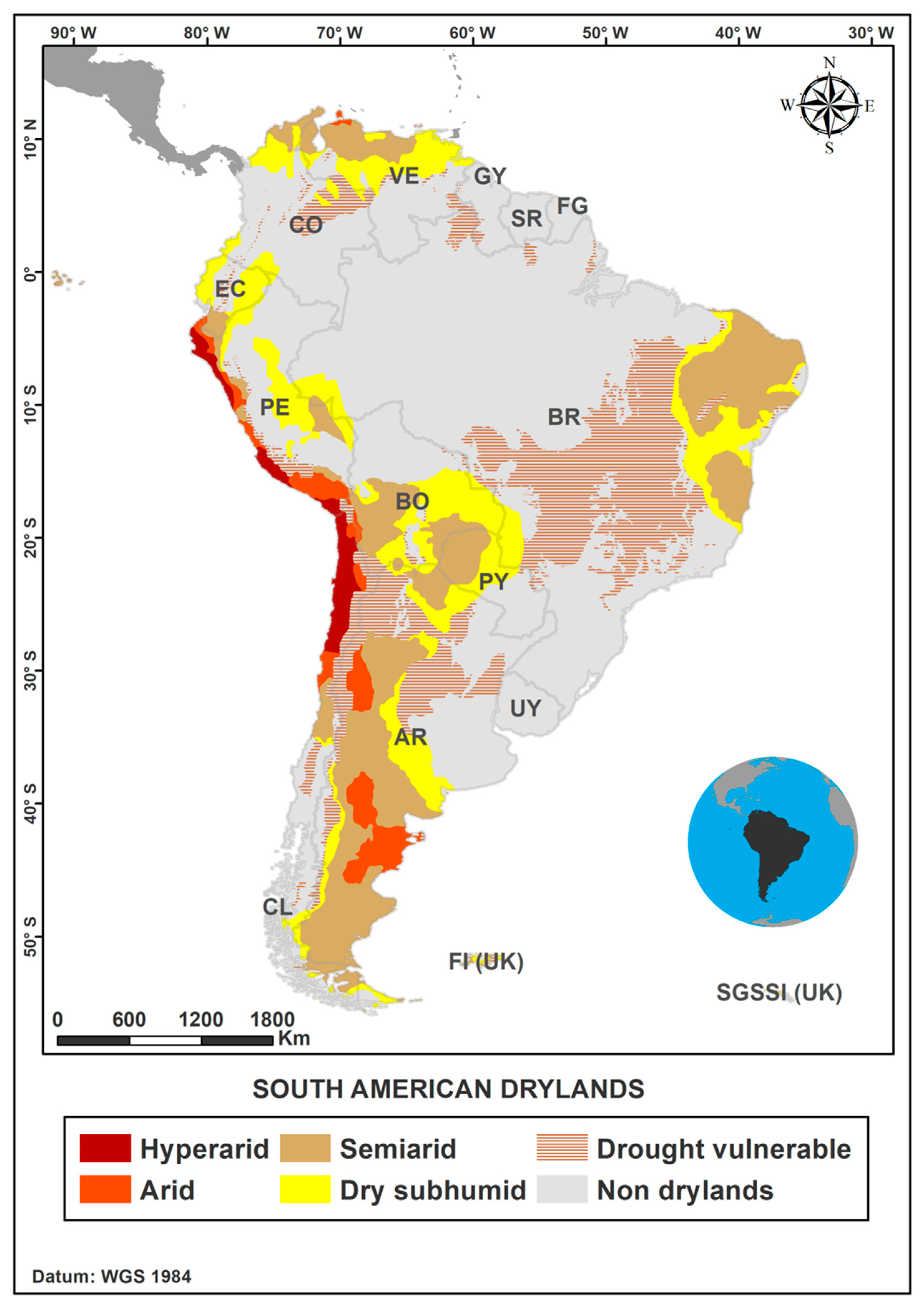
  • Hyperarid zone (AI < 0.05): areas with deficient and irregular seasonal rainfall and perennial vegetation restricted to shrubs in riverbeds. It is relevant to mention that we adjusted the boundary between hyperarid and arid zones to fit the definition we are following, given by UNEP-WCMC. UNESCO originally adopted a more restrictive threshold for this zone (AI < 0.03);
  • Arid zone (0.05 ≤ AI < 0.2): areas with annual rainfall between 80 and 350 mm, and perennial vegetation consisting of woody succulent, thorny or leafless shrubs;
  • Semiarid zone (0.2 ≤ AI < 0.5): areas with mean annual rainfall between 30 and 800 mm in the summer and between 200 and 500 mm in the winter at the Mediterranean and tropical latitudes; vegetation is composed of steppes, savannas, and scrubs;
  • Dry Subhumid zone (0.5 ≤ AI < 0.65): areas that comprise primarily tropical savannas and steppes.
Of the approximately 37 million square kilometers classified as semiarid and arid zones worldwide, 25.56 million (69%) refer to rangelands [44], where native vegetation either has been grazed or has the potential to be used to produce grazing livestock [45]. These landscapes occur in annual and perennial grasslands, shrublands, savannas, woodlands, and deserts [46]. In South America, Patagonian ecosystems from Argentina and Chile collectively constitute one of the world’s largest rangeland areas [47]. By and large, it is worth mentioning that not all rangelands are in drylands.

3. Study Area: South American Drylands

South America is the fourth largest continent worldwide, occupying 12% of the Earth’s land surface (17.8 million km2), with several regions and land cover types. Drylands are distributed among South American countries in different quantities, representing almost 80% of the Argentinian territory [10]. Table 1 lists the proportion of drylands to the whole country, continental, and global areas of each South American country where these ecosystems are found, at three different scales [10]. Guyana and Uruguay have a minimal portion of drylands covering their territory, while French Guyana and Suriname are the only countries within South America where drylands (or potential ones) are absent.
Following the UNEP-WCMC definition [43], four dryland subtypes are recognized in South America (Figure 1), covering an estimated 5.1 million km2 [10]. Semiarid is the most common dryland subtype (46%), followed by the dry subhumid (41%), arid (8%), and hyperarid (5%) zones [5]. The semiarid zone represents 14% of South America, with its highest country-level proportions found in Argentina (38%) and Brazil (9%) [10]. The most critical water-stressed subtypes are found in arid areas largely distributed over Argentina (70%) and the hyperarid regions predominantly in Chile (over 60%) and Peru (35%) [10].
Drylands in South America are primarily characterized by savannas, shrublands, woodlands, and grasslands [48], generally grouped into biomes. The high diversity of vegetation types is distributed over several South American ecoregions. The Caatinga is the driest forest of the continent, consisting of xeric shrubland and thorn woodland [49]. The Llanos (plains) del Orinoco is the second largest ecosystem of northern South America, encompassing parts of Venezuela and Colombia [50,51]. The sub-tropical shrubland in central Argentina, known as Espinal, is considered one of the most vulnerable ecoregions and is prone to LULC changes [52]. Concerning drylands that fall within the hyperarid classification, the Atacama Desert of northern Chile is broadly acknowledged as the driest globally [44]. Thus, it is used as one of the references for numerical thresholds for the extremely arid or hyperarid categories of AIs [53].
South America’s dry forest is less popular than the tropical rainforest [5]. However, the continent is predominantly covered with dry forests, including Tumbes-Piura in Ecuador and Peru, the Cauca, Magdalena, and Patía Valleys in Colombia, and parts of the Tumbes-Chocó-Magdalena biodiversity hotspots. Dry forests in South America occupy 199 million hectares, equivalent to 5% of the global forests and 18% of the worldwide dryland forest area [5].
Figure 1 also highlights drought-vulnerable areas (referred to as presumed drylands in the UNEP-WCMC dataset) [43,54]. Even though these areas do not reach the water deficiency level characteristic of drylands (displaying AI > 0.65), they include dryland features and/or dry and subhumid tropical forests [54], making them more prone to water stress. Drought-vulnerable areas such as the Cerrado, a seasonally dry tropical savanna, may experience reduced aridity in the near future due to the compounded effects of climate and land-use changes in the region [55,56,57]. Therefore, as a broad strategy to avoid drought-related ecosystems’ degradation, drought-vulnerable regions also need to be assessed and monitored. However, we did not include these areas in our review, which was limited to the four classes of drylands previously mentioned.

4. Literature Search and Selection of Sources

We performed a comprehensive review focused on identifying RS-based literature on LULC mapping initiatives of South America at various scales with an unlimited starting date until August 2021. We retrieved global, continental, national, and regional mapping studies from the Clarivate Analytics Web of Science scientific database (WoS, webofscience.com), last accessed 15 October 2021. We only considered peer-reviewed documents to ensure the authenticity and quality of the outcomes. Identifying these mappings created the basis for discussion around four issues of high relevance to drylands research: desertification, climate change, fire, and population.
The terms applied to the search were ‘Remote Sensing’, ‘Drylands’, and ‘South America’, and it was based on each study’s abstract/title/keywords. Articles about grasslands, savanna, shrubland, woodlands, and rangelands located in South America were more relevant for the search. Additionally, to increase the accuracy of the search, we filtered the initial search using the words ‘Global’, ‘Map’, and ‘Mapping’, as well as the names of countries and dryland ecoregions in South America. While screening, we selected the articles based on their titles, scope, objectives, and study area. The main goal was to identify RS-based vegetation mapping studies considering any portion of South America’s drylands. We then gathered information regarding five essential components of RS-based land cover mapping: mapping coverage, satellite datasets, classification techniques, legends, and validation protocols.
Initially, a total of 4142 publications from peer-reviewed journals were retained from the search process using the word “Drylands”. However, this total included all dryland regions across the world. By refining the process using multiple combinations and disregarding topics not related to remote sensing, we reviewed 59 papers. We added 25 studies to the initially retrieved sources after looking at their reference lists in the revision process, bringing the total number of sources used in this study to 84 papers. We disregarded grey literature because it consists primarily of reports that are not peer-reviewed and often not written in English.

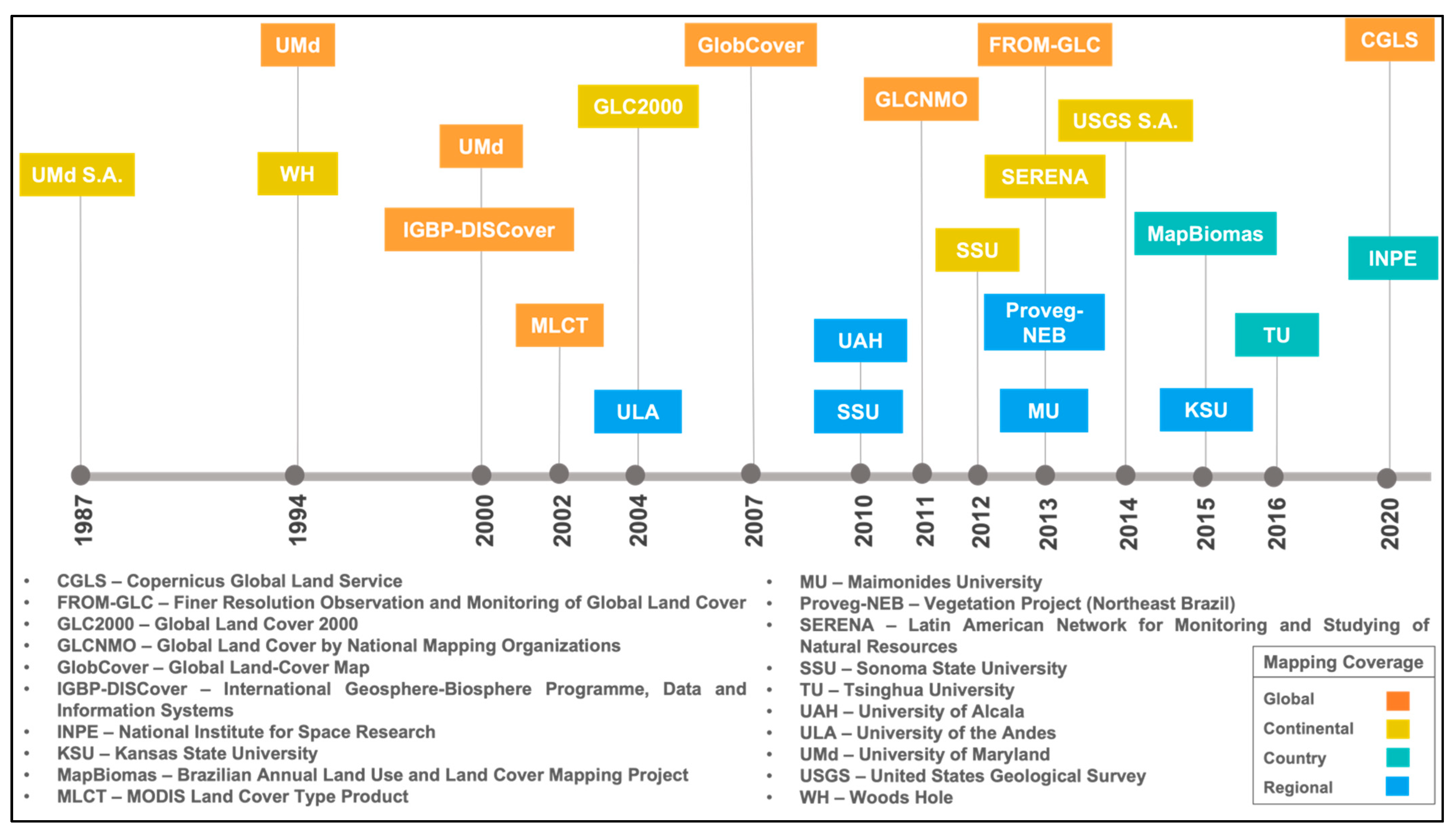
4.1. Mapping Initiatives in South American Drylands Using Remote Sensing

From the 84 studies we reviewed, we identified 23 initiatives that produced maps comprising South America, either entirely or partially (Figure 2). Among these initiatives, about 35% are global, 26% continental, 26% regional, and 13% national (with maps only for Brazil and Chile). We did not find country level maps for Argentina, Paraguay, Bolivia, and Peru, countries with a considerable presence of drylands. Regionally, only a few studies focused on mapping specific ecoregions, such as the Gran Chaco, Espinal, Llanos del Orinoco, and Caatinga. The latter is part of the country-level map produced by the MapBiomas project (www.mapbiomas.org, accessed on 30 September 2021), which has specific working groups to map each Brazilian biome, despite being published as a national map.
Several initiatives have mapped South America’s land cover at the continental level since the early 1900s [58], mostly from multiple sources and built from techniques other than RS-based ones. All the vegetation maps from the 1970s and 1980s hold a climate element in the classification scheme and, therefore, symbolize a mix of current and potential land cover [59]. Since the late 1980s, South America’s vegetation maps have been produced from data collected systematically by Earth-Observation (E.O.) satellites (Table 2). They benefit from homogeneous observations across the continent and provide improved spatial detail. However, they do not share the same thematic richness as earlier products [59].
The first RS-based map of South America was produced by the University of Maryland. This product aimed primarily to provide improved information for the modeling community [60]. After a seven-year gap, the University of Maryland also produced the first global map. In the 2000s maps, the interval between the release of new LULC maps for South America reduced, and the first regional LULC map was produced in 2004 for Llanos del Orinoco, in Venezuela. This map remains the most significant contribution from RS to the country, which still lacks a country-level map published in the scientific literature. Around a decade later, the first 30 m resolution global land-cover map from Landsat (TM and ETM+) increased the level of detail for observation and monitoring at the global level [61], which was later improved [62]. The 2010s saw an increase in the number of maps at various scales, with an average of one map published every year. In 2015, the first nationwide mapping initiative took place in Brazil, taking full advantage of the historical Landsat series to generate annual LULC maps.
Table 2. Remote-sensing-based mapping efforts that include South American drylands.
Mapping
Coverage
Reference 1,2DatasetClassifierLegend 3Validation
GlobalCGLS [63]PROBA-VRandom Forest23 classesOverall Agreement/Confusion Matrix S
FROM-GLC [61,62]LandsatRandom Forest/Support Vector Machine26 classesConfusion Matrix R
GLCNMO [64]MODISMaximum Likelihood20 classesConfusion Matrix R
GlobCover [65]MERISUnsupervised22 classesConfusion Matrix R
IGBP-DISCover [66]AVHRRK-Means17 classesConfusion Matrix R
MLCT [67,68]MODISRandom Forest23 classesCross-validation
UMd (1994) [69]AVHRRMaximum Likelihood11 classesN/A
UMd (2000) [70]AVHRRDecision Tree14 classesOverall Agreement
Continental
(South America)
JRC SA—GLC2000 [71]VariousISODATA12 classesOverall Agreement/
Confusion Matrix S
SERENA [72]MODISC5.022 classesConfusion Matrix R
SSU [73]MODISRandom Forest8 classesConfusion Matrix R
UMd S.A. [74]AVHRRMaximum Likelihood16 classesOverall Agreement
USGS S.A. [75]LandsatRandom Forest7 classesConfusion Matrix S
WH [76]AVHRRUnsupervised39 classesReliability Ratings/
Visual Comparison
CountryMapBiomas—Brazil [77]LandsatRandom Forest27 classesConfusion Matrix S
INPE—Brazil [78]PROBA-VRandom Forest7 classesOverall Agreement S
TU—Chile [79]LandsatRandom Forest35 classesConfusion Matrix S
RegionalSSU—Dry Chaco [80]MODISRandom Forest8 classesConfusion Matrix
KSU—Paraguayan Chaco [81]MODISISODATA6 classesConfusion Matrix S
MU—Espinal [52]LandsatMaximum Likelihood8 classesConfusion Matrix
Proveg-NEB—Northeast Brazil [82]LandsatISOSEG7 classesVisual Comparison
UAH—Central Chile [83]LandsatMaximum Likelihood8 classesOverall Agreement/
Confusion Matrix
ULA—Llanos del Orinoco [84]AVHRRMahalanobis Distance8 classesConfusion Matrix
1 Acronyms refer to the name of the project, when available, or the name of the leading university of each study. Please refer to Figure 2 for the initiative’s full name. 2 Products with multiple versions are in their most updated collection. 3 The number of classes refers to the most detailed level of the classification scheme for products published in different papers. Dataset: AVHRR = Advanced Very High Resolution Radiometer; MERIS = Medium Resolution Imaging Spectrometer; MODIS = Moderate Resolution Imaging Spectroradiometer; PROBA-V = Project for Onboard Autonomy—Vegetation. Classifier: ISODATA = Iterative Self-Organizing Data Analysis. Note: the Unsupervised label indicates no specification for the classifier in the study. Validation: N/A = not described or not systematically validated. R Simple Random Sampling; S Stratified Random Sampling.

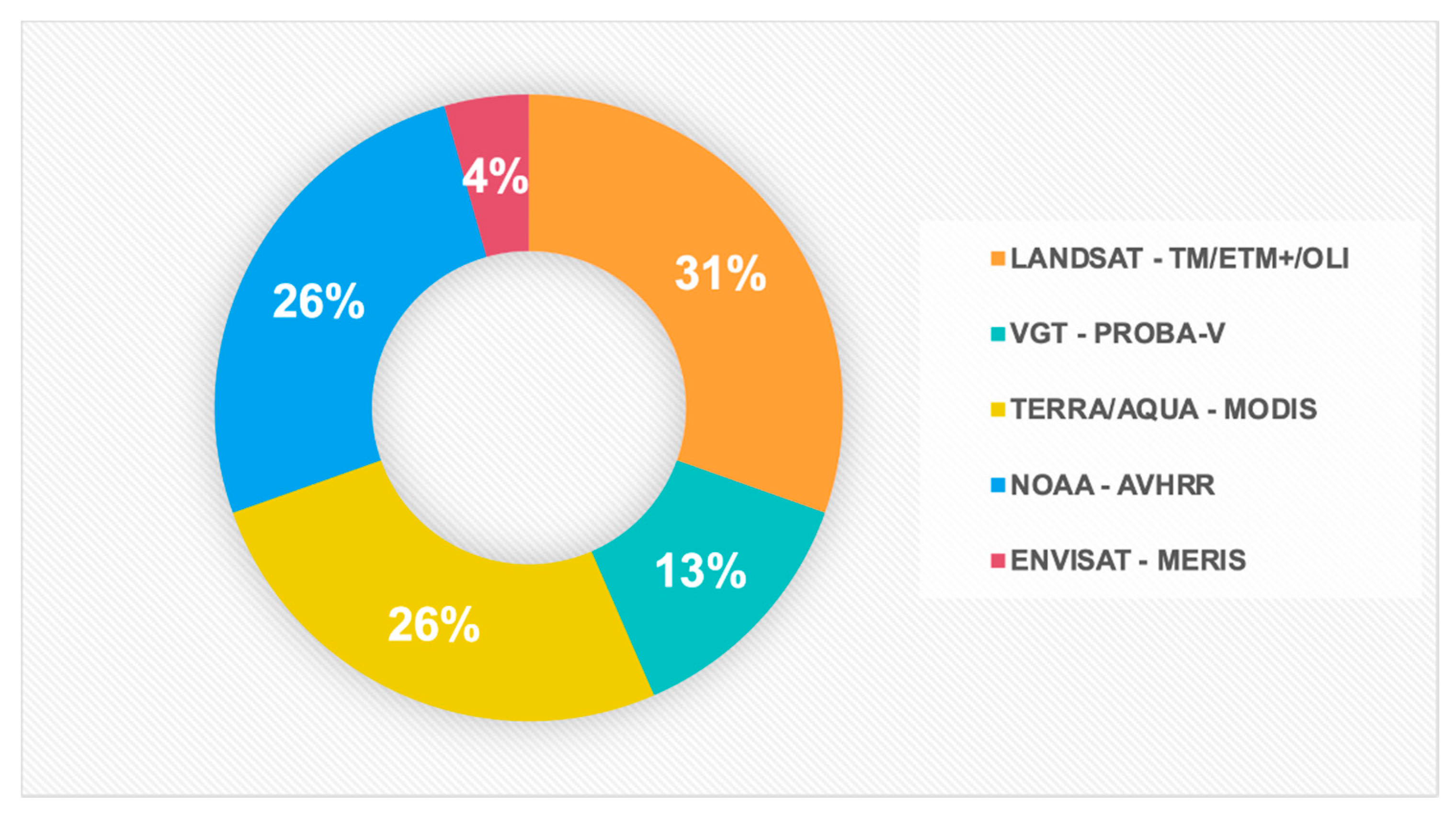
4.2. Remote Sensing Dataset

In most cases, satellite data are only available from the 1980s, so RS-based observations of LULC are only available from the last 40 years. In the 1990s and early 2000s, both MODIS and AVHRR were used to develop global land cover classification at the 1 km pixel resolution. Nowadays, multiple Earth observation datasets are available, with distinct spectral, spatial, and temporal resolutions [85]. Even with freely available fine-resolution datasets, dryland mapping initiatives (Table 2), including the most recent ones, used medium to coarse spatial resolution satellite imagery. Therefore, maps including drylands can be found at 1 km (AVHRR, MODIS) [64,66,70,74], 500 m (MODIS) [68,72], 300 m (MERIS) [65], 250 m (MODIS) [73,80], 100 m (PROBA-V) [63], and 30 m (Landsat) [61,62,77] resolutions (Figure 3).
The joint NASA and USGS Landsat program prevails in most studies because it collects data at the exact spatial resolution and with similar spectral bands, enabling the mapping and monitoring of LULC changes [86]. The Landsat archive enables the assessment of more than 30 years of images to monitor phenological changes and how they affect productivity at the regional and local levels. Since 2008, Landsat data became free and open, facilitating the application of its consistent imagery format in various fields [87].
Some studies chose the MODIS dataset possibly due to its temporally denser availability compared to Landsat. The MODIS-derived products used in dryland mappings were MOD13Q1 Vegetation Indices [80,81], MOD09GA [72], MOD43B4 NBAR [64], and collection 6 of MDLC (involving a combination of multiple MODIS products: MCD43A2, MCD43A4, MCD12Y3, MCD44W, and MCD44B). It is also noteworthy that most of South America’s LULC maps are not time-series based. The exceptions are two initiatives that release annual maps from the MODIS Land Cover Type Product (global level) and MapBiomas (country level). MapBiomas has mapped the most extensive period compared to all existing initiatives at the national level, with yearly maps starting from 2017 and going backward to 1985, spanning more than 30 years of coverage.

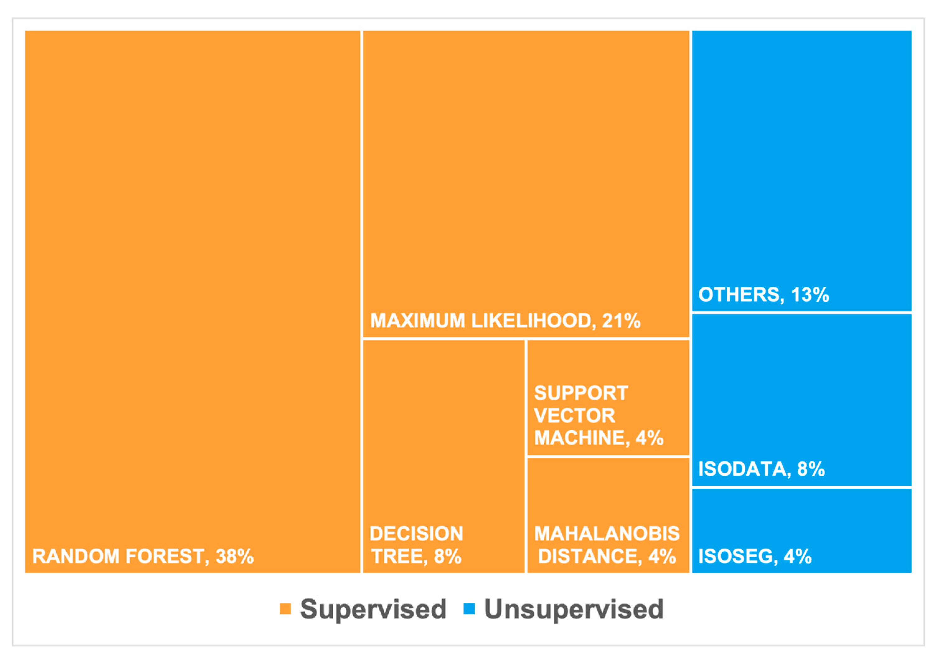
4.3. LULC Classification Methods

RS-based classification is recognized as the most efficient method of LULC mapping [88]. It has mainly been employed using a pixel-by-pixel approach, even though cloud cover remains a major cause of missing data [89]. Corrective pre-processing is a fundamental first step to minimize the cloud effects and other sources of noise and avoid interpretation problems. For instance, there was a consensus between authors in the reviewed studies that atmospheric correction is a requirement to improve the retrieval of surface reflectance, vegetation indices, and many ecosystems’ structural and functional properties, such as leaf area index (LAI). It is important to note that our review here is focused on aspects related to classifier development, even though there are other requirements for image classification (i.e., legend definition, input data generation, and sample data preparation).
The studies at the global/continental level described in Table 2 were notably different from the dryland’s spatial distribution shown in the reference map (Figure 1). Such a gap may be a consequence of the lack of compatibility among all satellite datasets and the classification approaches used. Among the techniques, supervised classification was the most applied, among which machine learning algorithms prevailed (Figure 4). Random Forest has undoubtedly shown a higher potential to improve the accuracy in dryland vegetation classification studies, besides controlling for over-fitting. Random Forest fits several decision trees using subsets of training samples and integrates predictions of the individual trees. The accuracy of a machine learning-based classifier such as Random Forest, for instance, highly depends on the quality level of the training samples [85] and the parameters of the classifier require preliminary experiments for definition, taking into account a fair balance between prediction performance and cost in computation time [79]. About a third of the studies (Table 2) used the Random Forest classifier, including all three country-level maps.
The Support Vector Machine was another machine learning-based classifier employed in South American drylands. It is a non-parametric algorithm applied to pattern recognition and classification that can generalize well even with a limited number of training samples [90]. Only FROM-GLC global mapping [61] used the Support Vector Machine, and its overall accuracy for level 1 and level 2 classifications (64.9% and 52.7%, respectively) was slightly higher than Random Forest’s (59.8% and 46.6%, respectively). However, after improving their methodology with segment-based pre-processing and a significantly higher number of input features to run the classification, the overall accuracy of both classifiers increased and became similar for both levels 1 and 2 (Support Vector Machine = 66.31% and 54.12%, respectively, and Random Forest = 67.08% and 54.6%, respectively). This example shows that the accuracy of the classification is not only a matter of defining the best classifier, but rather a combination of different analysis approaches, including legend definition, input data generation, and sample data preparation. We also identified unsupervised methods applied for LULC classification in South America. The ISODATA technique, for instance, was chosen to map the Paraguayan Chaco due to the lack of reliable training data. Despite that, the classification obtained a high overall accuracy of 84% [81].
LULC change detection is the process of detecting disparities in the state of an object or phenomenon on time-based observation [91]. This technique was applied in small-scale studies over South America’s drylands [52]. The use of time-series vegetation indices as an additional source in the mapping process was a trend in all existing coarse-resolution global land cover products. The two main indices were the Normalized Difference Vegetation Index (NDVI) [66,69,70] and the Enhanced Vegetation Index (EVI) [67,70]. However, each of these indices has advantages and disadvantages for in terms of better representing drylands in a map. Among these indices, EVI [92] responds well to chlorophyll, quantifies water-use efficiency, and tolerates background reflectance, but does not vary much over drylands. NDVI [93] is suitable to monitor phenology and long time series, but is not sensitive to woody components. Once used as metrics to run machine learning-based algorithms (e.g., Random Forest), these indices tend to increase the accuracy of classifications given that reliable training samples are available. In the scientific literature, other indices not previously used for mapping drylands are worth testing to classify drylands, such as the Normalized Difference Water Index (NDWI) [94] and the Modified Soil-Adjusted Vegetation Index (MSAVI) [95].
The pros and cons of using each of these indices will reflect the classifier’s ability to identify the diverse types of sparse vegetation formations in drylands. That is mainly because estimating vegetation cover depends on the inverse relationship between reflectance and plant cover or spectral indices and vegetation greenness. In the wavelength range relevant for plant detection (between 400 and 2500 nm), the main canopy-related factors influencing the reflected radiance are the optical properties of both the vegetation and the environment around the canopy (e.g., soil and atmosphere) and how these elements are arranged in the vegetation canopy [96]. In desert environments, changes in the mix of palatable and unpalatable grasses and bush dominance negatively impact changes in the vegetation structure [97]. Thus, conducting studies using different vegetation indices and informing the positive outcomes, setbacks, and failed results may help advance the identification of the heterogeneity of vegetation formations in drylands. Unmixing methods, such as those used by MapBiomas and INPE, can overcome some of these difficulties when dealing with complex systems. The spectral mixture analysis (SMA), which is an image transformation technique rather than a classifier [98], retrieves the relative abundance of each pixel’s endmember based on the inversion of a mixture model [34]. In this regard, the sensitiveness of the multiple endmember spectral mixture analysis (MESMA) [99] to changes in the spectral albedo makes this method a suitable choice for drylands [34].

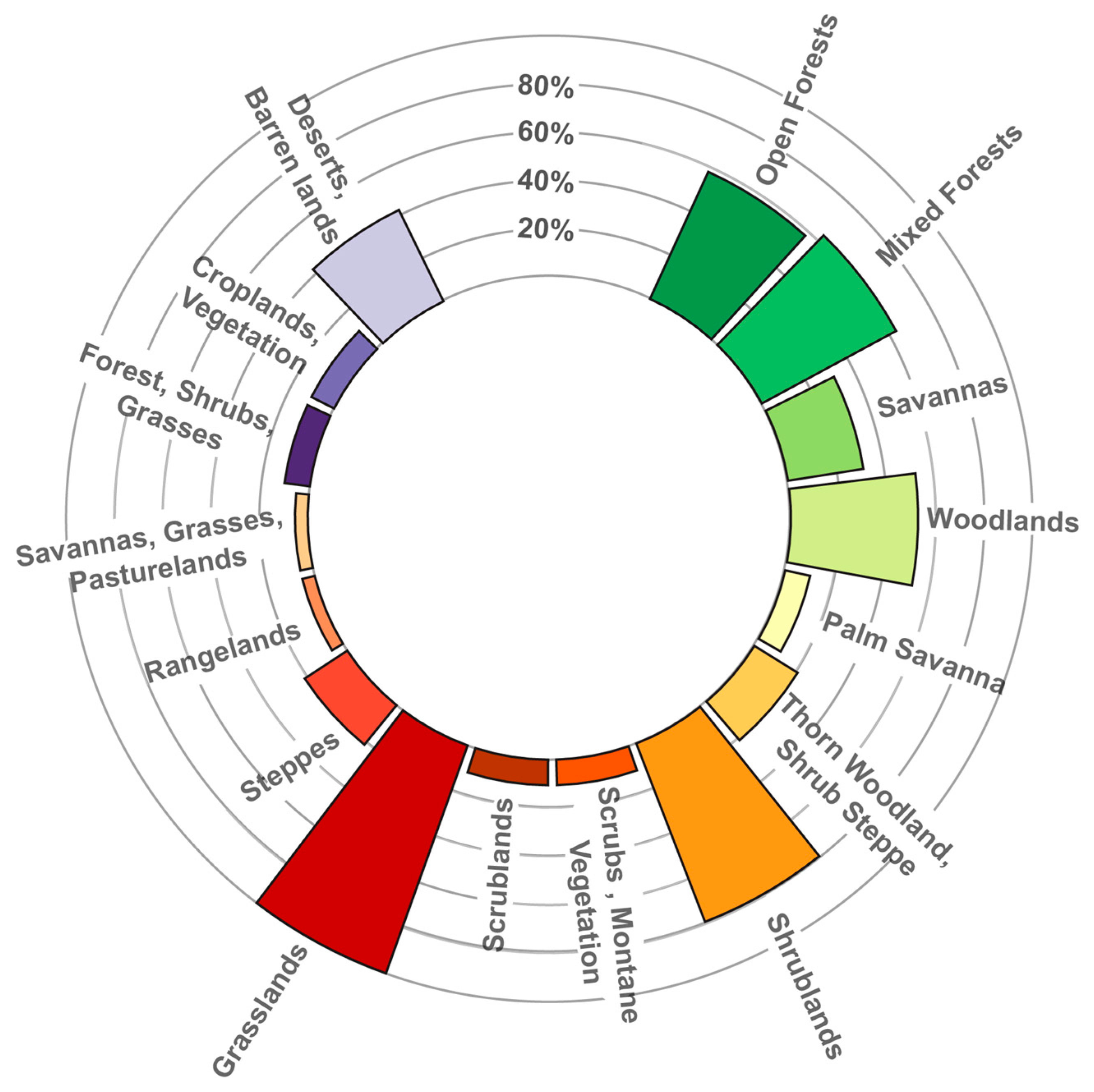
4.4. Classification Schemes

The lack of standardization is one of the main issues for classification legends [60]. This is particularly true for drylands. A common issue observed in the legends of most global maps is that woody vegetation in drylands lacks adequate representation because it often does not fulfill the criteria of ‘forest’ [48]. In addition, some drylands are represented in global LULC maps as large homogeneous areas and do not reflect the reality of vegetation distribution in these landscapes, as proved by regional-scale maps [84]. Detecting specific dryland formations is challenging at lower resolutions as each pixel contains more than one land cover type [80]. Such spectral confusion impacts classification scheme decisions and omits typical dryland formations from the final maps. Overall, our work found classification schemes ranging from 1 to 14 dryland classes in each one of the 23 maps analyzed. A more detailed analysis of each map’s legend allowed us to detect approximately 50 different names for dryland classes. After grouping similar classes (e.g., herbaceous vegetation and natural grassland, or barren lands and deserts), we found 16 dryland vegetation types in South American maps, among which grasslands, shrublands, mixed forest, open forests, and (woody) savannas are the most common (Figure 5).
A striking feature when comparing the legends of all studies in Table 2 is a direct relationship between the mapping coverage area and the number of classes in the legend, meaning that the smaller the mapping coverage area, the lower the number of classes. There are exceptions in the South American map produced by Woods Hole [76], the broadest classification scheme, with 39 classes, and the country-level maps of Brazil [77] and Chile [79], with 27 and 29 classes, respectively. Both national maps used Landsat imagery to perform LULC classifications, which explains the more detailed classification scheme. Regionally, the Paraguayan Chaco map showed the most representative number of dryland classes [81]. Even with only six classes, the final product sufficiently represented the different formations present in the study area (dry forest, xeric woodlands, scrublands, rangelands, savannas, and grasslands). Other regional maps did not have a similar level of detail (e.g., Espinal, Llanos, Dry Chaco, and Northeast Brazil).
International harmonization initiatives have provided subsidies for increasing the agreement on LULC characterization standards. The most robust methodology from the analyzed initiatives was implemented in the MCD12Q1 product from MLCT and includes the use of six classification schemes (such as IGBP and UMd). The classification schemes used by the MODIS Land Cover Type Product and the University of Maryland products follow the International Geosphere-Biosphere Programme (IGBP) classification system with 17 classes, whereas GLC2000 and GlobCover adopted a 22-class scheme developed for global modeling purposes by the IGBP system. The FAO/UNEP Land Cover Classification System (LCCS) has also been widely used as the primary source for defining the maps’ legends. However, the existing classification schemes have significant limitations in terms of the adoption of a classification system that considers vegetation traits, life-form information, and structure [61]. Such a gap reinforces the importance of developing classification keys targeting drylands and taking regional knowledge into account.

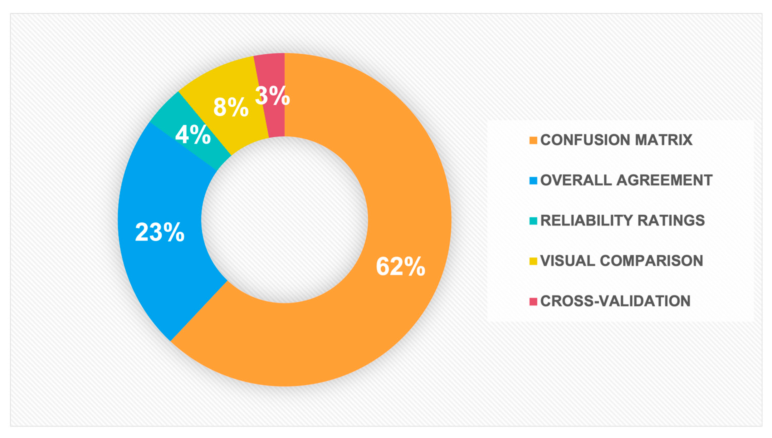
4.5. Validation Strategies

Ground referencing data for calibration and validation are necessary to map LULC [88] and reveal the quality of the outcomes for operational applications [100]. To meet the requirements of the user community, the accuracy of science products must be clearly informed. The validation of land cover products requires appropriate sampling strategies for the statistical assessment of accuracy, and the difficulty is even greater for larger areas due to limitations in cost and logistics [30]. Moreover, the reference data must be reliable enough to enable robust validation.
The first step of the accuracy assessment is generating the validation sample set and determining the sample size through methods such as the multinomial distribution function [101]. Typically, the number of samples is limited by the operational constraints of a study and often represents a compromise between the need to obtain a precise measurement and the requirement to remain efficient and able to process all samples adequately. More than 60% of the maps described in Table 2 used the confusion matrix to assess the accuracy (Figure 6). This method is based on nonspatial statistics and is effective for identifying classes that cause confusion and are potential sources of error. Furthermore, the confusion matrix provides quantitative and easy-to-interpret metrics, such as the user’s accuracy, producer’s accuracy, and overall accuracy.
The quality of sampling is also an essential aspect. When comparing South America’s dryland mapping initiatives, we found sampling approaches varying between simple and stratified random distribution. Stratified sampling is conducted by taking (randomly) the same number of points for each class. This method was applied by IGBP DISCover, and required extensive post-classification stratification to minimize confusion between distinct land cover types [66].
Concerning data collection, LULC samples were collected from fieldwork by mapping initiatives such as Maimonides University—Espinal [52] and the University of the Andes—Llanos del Orinoco [84] (primarily based on ground control points). FROM-GLC [61] products were based on training and test samples collected visually from Landsat images, using high-resolution images and field photos found in Google Earth as references. Kansas State University’s regional classification of the Paraguayan Chaco [81] used both data collected from ground points and high-resolution satellite images.

5. Discussion

Understanding the spatial distribution of dryland vegetation across South America at a higher level of detail is of utmost relevance for advancing research and governance in different topics. LULC mapping can help solve important issues that affect humanity and methodological advancements should be tuned to the current socioecological challenges. South American mapping initiatives contributed to understanding the implications of major transformations, at all scales, taking place over dryland ecosystems and populations, but there is still much to advance. We selected four topics often addressed in South American dryland mapping publications to exemplify how RS methodological advancements can help to address relevant environmental problems drylands face nowadays: desertification, climate change, fire mapping, and the resilience of the population in these fragile ecosystems.

5.1. Desertification

Land degradation is defined as the reduction in or loss of land’s biological or economic productivity [6]. The United Nations Convention to Combat Desertification (UNCCD) refers to desertification as land degradation in drylands [102], among which semiarid and arid regions are particularly vulnerable. This long-lasting process is driven by the complex interactions of anthropogenic and climate-induced factors [7]. Although some forms of desertification may be irreversible, policy and technical solutions combined with local and traditional knowledge sources can put these areas back on the track of productivity and sustainability [13].
Considering the absence of a standard assessment and monitoring system of desertification (either for South America or globally) [103], a recent low-resolution estimate puts South America among the most affected continents worldwide. Argentina and Brazil have the highest spatial extents of drylands experiencing desertification processes [12], and Argentina is specially affected with negative repercussions to varying degrees [104,105]. In Bolivia, Peru, Ecuador, and Chile, the problem affected between 27% and 43% of the land area [13]. Few assessments were produced to map problem areas, develop indicators, and evaluate political and economic needs to control desertification [106,107]. In this regard, the NDVI is often the primary RS metric [108,109], considered one of the most robust and independent alternatives for analyzing land productivity [102], even with its limitations. However, quantifying desertification remains a difficult task given the diversity and complexity of its processes [110]. There is also a lack of agreement about tipping points that, once reached, could lead to irreversible degradation over dryland ecosystems [111] or make restoration economically unfeasible. As the information on desertification in South America remains insufficient [112], some questions arise. How can RS accurately map the extent of desertification in South America? Which countries in South America have been mostly affected by this problem? What indicators directly measured by RS could deliver better information about the status of dryland degradation?
An essential first step to tackle these issues is coupling RS with country-level biophysical and socioeconomic data, enabling the development of a baseline and an integrated database. It is also important to involve regional experts and affected peoples in a broadly inclusive process to select indicators of desertification. Good results were achieved using satellite-based imagery analysis on vegetation loss, erosion [113], and drought monitoring [114], complemented by ground-based observations, which tend to provide consistent and cost-effective data to measure desertification. Careful calibration is also an important aspect, although many cloud-free images are available for drylands as they experience low humidity [115]. Such an advantage allows for consistent high-resolution imagery-based validation protocols on desertification products against field data [116]. Therefore, South American countries must have access to affordable satellite imagery to effectively implement integrated practices for mapping, assessing, and quantifying desertification.
In the scope of RS, a significant challenge is to segregate sparsely vegetated areas from those degraded by human impact [117]. A pressing issue is the differentiation of rangelands from converted pasturelands, as evidenced by a recent comparison of the world’s land degradation datasets [117]. In South America, Southern Brazil, Uruguay, and the Pampas of Argentina [117], where natural grasslands are abundant, showed the most significant disagreements. Further contributions from the RS community to this issue include correlations of LULC changes to the ecosystem’s carrying capacity indicators.

5.2. Climate Change

Overall, tropical dryland areas have faced temperature rises superior to the global average [118], and projections indicate that, during the 21st century, warming of 3.2–4 °C may occur over these areas (~44% higher temperature increase than in humid regions) [115]. Moreover, climate models also predict changes in the intensity and frequency of drought events [119,120], strongly affecting water-limited drylands. Anthropogenic LULC changes interact with the global climate system through complex feedback mechanisms. For example, accelerated desertification releases an estimated 300 million tons of carbon to the atmosphere yearly [6]. The emitted CO2 contributes to increasing global temperatures that, in turn, can drive the degradation process and desertification. In South America, developing countries with large dryland areas such as Argentina, Bolivia, Paraguay, and Chile are particularly vulnerable to climate change [121]. Even though increased atmospheric CO2 can fertilize drylands and cause vegetation greenness, water scarcity remains the leading climate change vector in most places, such as the Brazilian semiarid [118]. As the world faces novel and dynamic climate conditions, reliable and up-to-date mapping products for monitoring droughts are of utmost relevance.
According to the Global Climate Observing System (GCOS), 26 out of 50 essential climate variables (ECV) highly depend on satellite observations for more consistent climate studies [122]. Aerosol properties, albedo, carbon dioxide, leaf area index, and fire disturbance are among the variables of high relevance for dryland climate-related studies. These variables, once measured on the ground, are important to correct satellite RS retrievals [123]. Thus, map developers should ensure that classification schemes are detailed enough to suit the climate model’s requirements [124]. Such variables also contribute to the mapping of areas of ecological tension and the investigation of possible effects associated with anthropogenic climate change over drylands. In South America, RS mapping of LULC, combined with climate models, can improve our understanding of the land-atmosphere feedback mechanisms in drylands. It can also provide answers to complex questions at regional and local scales. Which ecosystems, populations, and economic activities are more vulnerable to climate change? Furthermore, how can climate change be adapted to, and greenhouse gas emissions be mitigated in South America’s drylands?
While answering these questions remains challenging, geoengineering techniques associated with solar radiation management and CO2 removal reveal feasible alternatives to minimize climate change-related economic setbacks and limit global warming [125]. Over drylands, solar energy is a high-incident renewable resource during the whole year [126]. Consequently, investigating potential areas for installing photovoltaic systems is a relevant mitigation strategy to combat climate change and generate income for vulnerable populations. In the scope of RS, how can satellite sensors support land assessment and monitoring for solar energy development in the drylands of South America? A research study conducted in drylands of the United States [127] successfully mapped solar energy potential using very high-resolution imagery and multiple vegetation indices (e.g., MSAVI and NDVI).

5.3. Fire Mapping

Natural and induced fires are drivers of soil conditions, land cover, and biodiversity changes. Drylands are susceptible to frequent fires [128,129,130]. They are pyrophytic open ecosystems [131], which, combined with topography, fuel composition, and ignitability, can accelerate the spread of fire and the probability of the occurrence of wildfire [132,133]. Globally, drylands comprise most of the estimated 420 Mha of land burned each year [134]. In addition, during 2020, South America showed the highest number of detected fires since 2011 [135]. However, fire occurrence and hazards in the continent’s drylands remain understudied [136]. Even for Gran Chaco, the largest dry forest in South America, few studies have investigated fire drivers [137,138]. As the climate becomes hotter and more intense, droughts may affect some drylands, and thus, there is a pressing need to improve fire mapping and early warnings in these ecosystems [139].
Both infrared and thermal bands are the most appropriate for fire detection [140]. Satellite-derived datasets on fire occurrence allow us to understand the spatial–temporal distribution of burned scars [141] and estimate greenhouse gas emissions resulting from the burning of native vegetation [142,143]. In addition, detecting high-temperature hotspots using active fires also contributes to more effective near real-time monitoring [144]. For mapping burned areas, it is crucial to consider the spectral properties of the vegetation. When fire strikes the leaves, the reduction in the leaf area index decreases the near-infrared (NIR) reflectance, and the depletion in moisture promotes an increase in short-wave infrared (SWIR) reflectance [145,146,147]. Due to the contrast obtained by the sharp drop in the NIR reflectance and the increase in the SWIR reflectance, the NIR/SWIR ratio has been widely used in spectral indices for fire detection and/or burning severity classification [148]. A study comparing the potential of 13 spectral variables for detecting burned areas observed a better correlation of field data with the Normalized Burn Ratio (NBR) index, calculated using the NIR and SWIR bands [149].
Several global burned area products have been developed at different temporal and spatial scales [134,141,150,151]. The remotely sensed burned area data products MCD45A1 and MCD64A1 from NASA’s MODIS instruments have the potential to map the spatial extent and approximate date of biomass burning worldwide at a spatial resolution of 500 m [134]. Additional alternatives for fire mapping and monitoring with coarse spatial resolution include the 250-m Fire_cci v5.0 products [141], ESA’s 1-km GLOBCARBON [152], and the 300-m and 1-km L3JRC Copernicus PROBA-V Burnt Area products [153]. In addition to these products, the launching of the Visible Infrared Imaging Radiometer Suite (VIIRS) sensor in 2011 represented a significant advance in fire monitoring. The sensor has specific bands for monitoring fire on the earth’s surface, providing data at 375 m spatial resolution, allowing the detection of smaller fires and a better refinement in the mapping of larger fires [154].
Combining RS data with machine learning algorithms seems to monitor fire activity adequately and contribute to landscape management and the identification of fire-prone areas. For example, the recently launched MapBiomas Fire [155] successfully mapped fire scars in Brazil, including the country’s drylands, over 36 years (1985–2020). This initiative is a pioneer in employing a deep learning-based approach at the national level in South America. A recent study modeling fire probability has been conducted in the Colombian–Venezuelan Llanos and used the random forest algorithm [136]. Such estimation must consider the location of the burned area and the causes of the fire spread. Another direction for fire research in drylands is to increase the efforts to build a regional scale modeling approach involving spatial information at a finer scale, which has been overlooked [136]. Regionally, the LPJmL4-SPITFIRE is a Dynamic Global Vegetation Model (DGVM) developed to simulate burnt areas [156] in Brazil’s most dryland fire-prone regions. Similar applications might prove helpful for other South American dryland ecoregions.
Fire mapping could help address some still unanswered questions. To what degree are South America’s drylands vulnerable to fire in a changing climate? What is the interval between fire occurrence and vegetation recovery in South American drylands? How may fire frequency be altering dryland’s biodiversity at different scales? A very recent study indicated that available information on the fire regime remains limited for the continent [157]. Therefore, studies focused on fire perimeters, in addition to the severity mapping and landscape controls of fires, would help advance our knowledge about fire in drylands and be powerfully supported by LULC maps. Further investigation on post-fire regeneration is also important, as it might take more than 40 years for woody ecosystems to recover [158,159].

5.4. Dryland Populations

According to the World Resource Institute (WRI), 30% of the South American population is settled in drylands [160]. In Brazil, more than 35 million people live in the Caatinga, whereas in Peru, approximately 88% of the country’s population live in drylands. Population growth puts unprecedented pressure on natural resources over drylands.
Populations in drylands are affected by the water-limited environment, especially those who depend directly or indirectly on agriculture for survival [13,161]. Dryland populations have learned to adapt to highly variable climate conditions by developing numerous technologies to make their livelihoods more resilient. However, climate change and desertification intensify the variability of environmental conditions, posing new threats to drylands and their inhabitants [19]. RS-based tools and LULC maps, coupled with social and demographic variables, could help enhance the adaptative capacity of dryland populations and promote the sustainable management of ecosystems. Investigation on erosion detection [162,163], drought-vulnerability [164,165] and cropland/pastureland [166] mapping is vital to inform policymaking to combat food insecurity and poverty [112]. These policies can also help to balance possible trade-offs between ecosystem services and economic growth in drylands.
RS-based LULC maps have long been used to map priority sites for conservation and restoration [52] while avoiding conflicts with agriculture and other land uses. Detailed and up-to-date information about under-protected ecosystems combined with LULC dynamics data could provide valuable information to increase drylands’ resilience by maintaining local biodiversity and increasing ecosystems’ multifunctionality [11]. From the hydrological point of view, considering that water is a critical limiting factor in drylands, RS maps were also used to understand potential water-use conflicts and the ways in which LULC and climate change affect water security [167]. However, information about conflicts is still scarce throughout South American drylands. Such information should target key vulnerable groups (e.g., migrating pastoralists) to reduce conflicts for natural resources and increase adaptative strategies.
A broader understanding of many themes requires advancements in RS techniques to surpass the limitations posed by the existing coarse- to medium-resolution products. More detailed maps may allow the representation and sharing of local communities’ technologies to adapt to water-limited conditions and increase land productivity [13]. Finer resolution data may also inform policies that favor risk-reducing strategies and secure property rights. Mapping at a more detailed level is pivotal to extrapolate the results of studies to the scale needed by farmers to decide how to manage their lands. In this way, technical and socioeconomic constraints can be reduced, while incentives for community participation in sustainable land management initiatives can be promoted, as made possible by a recent initiative from Argentina [168,169]. Their methodology combined collective mapping with GIS- and RS-derived parameters, including LULC. Such initiatives can collectively construct knowledge based on the interaction among local, governmental, and scientific communities to define priority areas for conservation across South America’s drylands.
In the future, RS may help address critical issues to answer some questions: What are the dryland vegetation conservation gaps in South America’s network of protected areas? Where will potential conflicts for water arise, and what are the most vulnerable groups? How do local populations perceive their environment, and what solutions have they developed to cope with water limitation? What are the main factors influencing farmers’ management decisions, and how can adequate incentives be offered to promote sustainable practices?

6. Methodological Trends and Current Challenges in Dryland Mapping

Current studies have been mainly conducted in some of the largest South American dryland ecosystems—Dry Chaco, Caatinga, and Llanos from Colombia and Venezuela. Meanwhile, smaller ecoregions have been underrepresented by RS studies. Such a challenge was corroborated by our results, which found only three and six studies at the national and regional scales, respectively. Unique dryland regions found in South America, such as the Monte Desert in Argentina [170], as well as other important ecoregions, remain understudied (Table 3).
To advance South America’s dryland mapping, major methodological challenges must be addressed in the future. The first is the strong spectral mixing, particularly in xeric formations, characterized by a mix of shrubs, grasses, and soil [34], which often results in a considerable influence of senesced or inactive vegetation and soil on the reflectance spectra. The second challenge is the high heterogeneity of drylands at many scales, which is mainly linked to the vegetation structure (e.g., the height and leaf area) and function (e.g., evergreen shrubs and deciduous shrubs) [8,34]. Such variability makes model parameterization considerably harder in moderate- to coarse-resolution imagery.
A third challenge is minimizing temporal divergences between the environmental process and observation scales [171]. For example, because there is a gap between vegetation green-up and the start of the growing season, vegetation activity following rain events may not be captured by spectral vegetation indices with lower temporal frequency [8]. Such a mismatch is commonly observed in single-time image maps. To meet these requirements, it is necessary to develop cost-effective ways to process satellite images and produce LULC maps with high temporal resolution. High-performance computing and machine learning algorithms have been increasingly used, making dryland vegetation mapping easier at the continent level.
The last challenge is the lack of ground-based data networks distributed across South America’s drylands to calibrate and validate RS algorithms. Readily available datasets of vegetation characteristics might provide comprehensive information on South America’s dryland ecosystems and contribute significantly to more compatible legends for future LULC maps. In this regard, a trending approach involves the use of databases of crowd-sourced field photos to collect geo-referenced images from different researchers. The Geo-Wiki project, for example [172], launched a mobile app in 2013 that enables the sharing of photographs with environmental information. Geo-Wiki has also vastly increased its database of in-situ information on land cover available for the training, calibration, and validation of LULC maps [173]. Similarly, the Global Geo-Referenced Field Photo Library [174], set up by the University of Oklahoma, contains more than 150,000 photographs taken on field with manually labeled land cover types.
A trendy free web-based tool that also supports data validation is the Temporal Vegetation Analysis System (SATVeg) [175], developed for instantaneously accessing temporal profiles of MODIS vegetation indices in South America. Systems of this kind help support numerous LULC monitoring activities, allowing quick queries and efficient updating [175]. Another noteworthy initiative is a field-based ecosystem monitoring protocol for Argentinian and Chilean Patagonia, called the Environmental Monitoring of Arid and Semiarid Regions (MARAS) network [47]. This dataset stores vegetation and soil data of 426 rangeland monitoring plots containing photographs, basic climatic and landscape features, and a line-intercept transect for vegetation spatial pattern analysis.
By and large, our study draws attention to the development of an integrated multi-level approach rooted in the concept of interoperability for mapping drylands. Such interoperability relates to South American experts’ joint use of land-cover information and the exchange of information from multiple datasets [176]. Both technically and institutionally, this approach remains challenging considering each country’s social reality and ability to invest in technical–scientific improvements. A key solution to advance this knowledge requires the establishment of multi-institutional cooperation agreements and the raising of funds to promote these efforts. As a result, future maps will have more compatible legends, trained interpreters, and clearer accuracy assessment protocols to improve their applicability in monitoring fire and drought and issuing early warnings that increase the ability of decision-makers to tackle the situation faster.
From the RS perspective, to make this integration more manageable, new-generation satellites and techniques have emerged as promising alternatives. For example, a data fusion approach harmonizing Landsat-8 and Sentinel-2 data successfully represented seasonal cycles of annual grasses vegetation greenness in the United States’ dryland ecosystems [177]. Once enhanced by field observations, biophysical variables, and machine learning techniques, this methodology accurately depicted annual grass cover using spatiotemporal resolutions that are useful to local resource management [177]. The low atmospheric influence of the synthetic aperture radar (SAR) data in the microwave spectrum range also increases their suitability for mapping and monitoring South America’s drylands. Sentinel-1, for instance, has generated open and free SAR images since 2014, which have been widely used to study African savannas [178,179]. Studies in South America’s drylands may also combine Sentinel-1 and Sentinel-2 for single-year vegetation mapping using high spatial resolution data and more detailed classification schemes. The narrow spectral bands of hyperspectral RS are also advantageous compared to the barriers faced by optical data. Upcoming imaging spectroscopy sensors that are satellite-based (e.g., HyspIRI, CHIME, EnMAP, PRISMA—recently launched—and SBG) or onboard of the International Space Station (ISS) (e.g., DESIS, EMIT, and HISUI) will allow large-area mapping [34]. These future satellite innovations will enable the upscaling of in situ data to be used as training data for the LULC mapping of South American drylands.
Methodologically, time series analysis brings new opportunities to investigate the dynamics of dryland vegetation. A novel generation of technological solutions has benefited from time-series analysis and satellite data integration to create RS-based Earth Observation data cubes [180]. Efforts of this kind were created in Armenia [181], Australia [182], Switzerland [183], and Brazil [85]. The Brazil Data Cube [85] tends to pave the way for expanding Earth Observation data to map dryland ecosystems in other South American countries. Such initiatives produce analysis-ready data, increasing access to larger communities of users and supporting decision-makers with information translated to significant biophysical metrics.
Among these metrics, land-surface phenology has arisen as a promising trend that enables more sophisticated land-cover mapping [62], playing a vital role in terms of the effectiveness of the study of dryland ecosystems [177]. In addition to the use of traditional satellite-based approaches, changes in phenological cycles can be assessed through unmanned aerial vehicles (UAVs) and phenology networks (e.g., PhenoCams). Repeated photographs taken from digital cameras on the ground or coupled in towers may effectively monitor plant phenology [184] and, thus, overcome the barriers posed by seasonality. Such a technique is referred to as near-surface remote sensing and was found to reveal an important link between plant phenology and conservation biology [185]. Although this approach has proved reliable in bridging field observations with those from satellites in dryland ecosystems, mainly in the United States [186,187], its usage in South America is still limited, with few studies conducted in Caatinga [188].
Products from phenological observations can be an input to climate models at various scales, contributing to model land-cover change scenarios under local and regional climates. Programs such as TIMESAT [189] are feasible to examine signals found in time series phenological data [80]. A phenology-based approach is a suitable solution to improve rangeland management [190] and enable researchers to overcome the challenge of segregating areas with natural low productivity or sparse vegetation from those that have been degraded by human impact.
To synthesize the main topics that we discussed in this paper, Table 4 gives an overview of the leading scientific landmarks of dryland vegetation mapping in the scope of remote sensing. We highlighted these advancements based on scale, datasets, classification techniques, classification schemes, and validation strategies. We divided the information across 3 different periods, from the late 1980s to the present, including pioneers in the study field, early mapping incursions and contemporary initiatives [191]. Additionally, the main challenges and trends also indicate the emerging horizons [191] in the scope of remote sensing LULC classification over South America’s drylands.

7. Concluding Remarks

We conducted the first comprehensive review, to our knowledge, of dryland vegetation mapping in South America. We identified 23 mapping initiatives, ranging from regional to global coverage. Although RS-based vegetation maps introduced a set of advantages, our study showed that the process of mapping LULC in South America has unfolded at a slow pace since the technology became available, with very few efforts directed towards drylands. Overall, there are more global maps (eight), followed by continental and regional maps (six each). Nationwide, there are only three maps (two for Brazil and one for Chile). We could not find RS-based LULC maps for Argentina, Bolivia, Colombia, Ecuador, Paraguay, Peru, Uruguay, and Venezuela. Regional cooperation to overcome national challenges is fundamental to advance the knowledge of the continent’s vegetation dynamics in its entirety, in addition to providing more consistent information for subsidizing policymaking at the regional scale.
Our study also showed that, although almost all global and continental maps have been produced from optical, coarse-resolution remote sensing, they are not easily comparable. Consequently, it is still challenging to combine these different products effectively to improve their application in themes that are highly relevant to drylands. It is also noteworthy that the spatial and temporal heterogeneity of vegetation plays a major role in dryland mapping. This issue may be solved using remote sensing products with high spatiotemporal resolutions (e.g., Sentinel). Concerning the use of spectral vegetation indices, instead of investigating the most suitable ones for dryland vegetation mapping, future methodologies should look for ways to explore the potential of adding multiple indices as inputs in machine learning-based classification algorithms (e.g., Random Forest). This multi-feature approach is a promising methodological trend for improving the differentiation of LULC classes that are easily mixed. Indeed, machine learning-based algorithms coupled with strengthening accuracy assessment procedures assure high-quality products to fulfill the needs of users from the public and private sectors.
A comparative overview of the methodologies and the validation procedures is required to support users’ decision-making on which dataset to use. From the available maps, MapBiomas stands out for its robust method and multiple-application products at the country level, given its medium spatial resolution. So far, sensors from the Landsat series have performed better at mapping drylands. The results of MapBiomas demonstrated the potential of Landsat for LULC mapping. However, limitations in resolution are likely to be overcome with new sensors in future studies. For future research, we strongly suggest exploring phenology, differentiating between natural and human effects, as well as using auxiliary data such as bioclimatic variables, the digital elevation model (DEM), and zoning data to improve remote sensing LULC classification and make it more practical. By incorporating such environmental gradients, better conditions for their public recognition and wide applicability in South America’s dryland ecosystems will be created. In addition, overcoming the incorrect notion that drylands resemble desert places of low economic interest, with scarce biodiversity, is necessary to attract more scientific interest to these regions.

Author Contributions

Conceptualization, K.A.G.; methodology, K.A.G., A.d.A.R., M.T.d.O. and Y.X.; formal analysis, K.A.G.; resources, Y.X. and Y.E.S.; writing—original draft preparation, K.A.G., A.d.A.R., M.T.d.O., N.S.d.C. and A.C.D.; writing—review and editing, Y.X., W.F.-R., E.Y.T.C., M.R.R., A.C.D. and Y.E.S.; visualization, K.A.G., A.d.A.R., M.T.d.O. and N.S.d.C.; supervision, Y.X. and Y.E.S. All authors have read and agreed to the published version of the manuscript.

Funding

This research was funded by Coordenação de Aperfeiçoamento de Pessoal de Nível Superior (CAPES), grant numbers 001 (A.d.A.R. & N.S.d.C.) and 88887.600358/2021-00 (A.C.D.); Conselho Nacional de Desenvolvimento Científico e Tecnológico (CNPq), grant numbers: 141988/2020-7 (A.d.A.R.), 444327/2018-5 (K.A.G.), 140378/2018-9 (M.T.d.O.), 140379/2018-5 (N.S.d.C.), and 431172/2018-8 (Edital Universal) (Y.E.S.); MapBiomas Project (W.F.-R); and U.S. National Aeronautics and Space Administration (NASA) Grant 19-SMAP19-0018 (Y.X.).

Data Availability Statement

No new data were created or analyzed in this study. Data sharing is not applicable to this article.

Acknowledgments

The authors would like to thank the National Institute for Space Research (INPE), the State University of Feira de Santana (UEFS), and the University of Brasilia (UnB) in Brazil; the National Institute for Glacier and Mountain Ecosystem Research (INAIGEM) in Peru; and the National Aeronautics and Space Administration (NASA), as well as the Department of Geography at the University of California, Los Angeles (UCLA), in the United States.

Conflicts of Interest

The authors declare no conflict of interest and the funders had no role in the design of the study; in the collection, analyses, or interpretation of data; in the writing of the manuscript, or in the decision to publish the results.

References

  1. United Nations Convention to Combat Desertification. Valuing the Biodiversity of Dry and Sub-Humid Lands; Technical Series No. 71; Secretariat of the Convention on Biological Diversity: Montreal, QC, Canada, 2013. [Google Scholar]
  2. Davies, J.; Poulsen, L.; Schulte-Herbrüggen, B.; Mackinnon, K.; Crawhall, N.; Henwood, W.D.; Dudley, N.; Smith, J.; Gudka, M. Conserving Dryland Biodiversity; IUCN: Cambridge, UK, 2012; p. 101. [Google Scholar]
  3. Gudka, M.; Davies, J.; Poulsen, L.; Schulte-Herbrüggen, B.; MacKinnon, K.; Crawhall, N.; Henwood, W.D.; Dudley, N.; Smith, J. Conserving Dryland Biodiversity: A Future Vision of Sustainable Dryland Development. Biodiversity 2014, 15, 143–147. [Google Scholar] [CrossRef]
  4. Xue, Y.; Hutjes, R.W.A.; Harding, R.J.; Claussen, M.; Prince, S.D.; Lebel, T.; Lambin, E.F.; Allen, S.J.; Dirmeyer, P.A.; Oki, T. The Sahelian Climate. In Vegetation, Water, Humans and the Climate; Kabat, P., Claussen, M., Dirmeyer, P.A., Gash, J.H.C., de Guenni, L.B., Meybeck, M., Pielke, R.A., Vörösmarty, C.I., Hutjes, R.W.A., Lütkemeier, S., Eds.; Global Change—The IGBP Series; Springer: Berlin/Heidelberg, Germany, 2004; pp. 59–77. ISBN 978-3-642-62373-8. [Google Scholar]
  5. FAO—Food and Agriculture Organization of the United Nations. Trees, Forests and Land Use in Drylands: The First Global Assessment: Full Report; FAO Forestry Paper No. 184; FAO: Rome, Italy, 2019; ISBN 978-92-5-131999-4. [Google Scholar]
  6. Millennium Ecosystem Assessment. Ecosystems and Human Well-Being: Desertification Synthesis; World Resources Institute: Washington, DC, USA, 2005; ISBN 978-1-56973-590-9. [Google Scholar]
  7. Wang, L.; D’Odorico, P.; Evans, J.P.; Eldridge, D.J.; McCabe, M.F.; Caylor, K.K.; King, E.G. Dryland Ecohydrology and Climate Change: Critical Issues and Technical Advances. Hydrol. Earth Syst. Sci. 2012, 16, 2585–2603. [Google Scholar] [CrossRef] [Green Version]
  8. Smith, W.K.; Dannenberg, M.P.; Yan, D.; Herrmann, S.; Barnes, M.L.; Barron-Gafford, G.A.; Biederman, J.A.; Ferrenberg, S.; Fox, A.M.; Hudson, A.; et al. Remote Sensing of Dryland Ecosystem Structure and Function: Progress, Challenges, and Opportunities. Remote Sens. Environ. 2019, 233, 111401. [Google Scholar] [CrossRef]
  9. Lian, X.; Piao, S.; Chen, A.; Huntingford, C.; Fu, B.; Li, L.Z.X.; Huang, J.; Sheffield, J.; Berg, A.M.; Keenan, T.F.; et al. Multifaceted Characteristics of Dryland Aridity Changes in a Warming World. Nat. Rev. Earth Environ. 2021, 2, 232–250. [Google Scholar] [CrossRef]
  10. Prăvălie, R. Drylands Extent and Environmental Issues. A Global Approach. Earth-Sci. Rev. 2016, 161, 259–278. [Google Scholar] [CrossRef]
  11. Maestre, F.T.; Quero, J.L.; Gotelli, N.J.; Escudero, A.; Ochoa, V.; Delgado-Baquerizo, M.; García-Gómez, M.; Bowker, M.A.; Soliveres, S.; Escolar, C.; et al. Plant Species Richness and Ecosystem Multifunctionality in Global Drylands. Science 2012, 335, 6. [Google Scholar] [CrossRef] [Green Version]
  12. Burrell, A.L.; Evans, J.P.; De Kauwe, M.G. Anthropogenic Climate Change Has Driven over 5 Million km2 of Drylands towards Desertification. Nat. Commun. 2020, 11, 3853. [Google Scholar] [CrossRef]
  13. Mirzabaev, A.; Wu, J.; Evans, J.; García-Oliva, F.; Hussein, I.A.G.; Iqbal, M.H.; Kimutai, J.; Kmowles, T.; Meza, F.; Nedjraoui, D.; et al. Desertification. In Climate Change and Land: An IPCC Special Report on Climate Change, Desertification, Land Degradation, Sustainable Land Management, Food Security, and Greenhouse Gas Fluxes in Terrestrial Ecosystems; Intergovernmental Panel on Climate Change: Geneva, Switzerland, 2019. [Google Scholar]
  14. Stringer, L.C.; Reed, M.S.; Fleskens, L.; Thomas, R.J.; Le, Q.B.; Lala-Pritchard, T. A New Dryland Development Paradigm Grounded in Empirical Analysis of Dryland Systems Science. Land Degrad. Develop. 2017, 28, 1952–1961. [Google Scholar] [CrossRef] [Green Version]
  15. Middleton, N. Deserts: A Very Short Introduction; Oxford University Press: New York, NY, USA, 2009; ISBN 978-0-19-956430-9. [Google Scholar]
  16. Adeel, Z.; Bogardi, J.; Braeuel, C.; Chasek, P.; Niamir-Fuller, M.; Gabriels, D.; King, C.; Knabe, F.; Kowsar, A.; Salem, B.; et al. Re-Thinking Policies to Cope with Desertification. 2007. Available online: https://www.pseau.org/outils/ouvrages/inweh_policies_to_cope_desertification.pdf (accessed on 1 October 2021).
  17. Schwilch, G.; Liniger, H.P.; Hurni, H. Sustainable Land Management (SLM) Practices in Drylands: How Do They Address Desertification Threats? Environ. Manag. 2014, 54, 983–1004. [Google Scholar] [CrossRef] [Green Version]
  18. Lal, R. Carbon Cycling in Global Drylands. Curr. Clim. Chang. Rep. 2019, 5, 221–232. [Google Scholar] [CrossRef]
  19. Xue, Y. Interactions and Feedbacks between Climate and Dryland Vegetations. In Dryland Ecohydrology; D’Odorico, P., Porporato, A., Wilkinson Runyan, C., Eds.; Springer International Publishing: Cham, Switzerland, 2019; pp. 139–169. ISBN 978-3-030-23268-9. [Google Scholar]
  20. Poulter, B.; Frank, D.; Ciais, P.; Myneni, R.B.; Andela, N.; Bi, J.; Broquet, G.; Canadell, J.G.; Chevallier, F.; Liu, Y.Y.; et al. Contribution of Semi-Arid Ecosystems to Interannual Variability of the Global Carbon Cycle. Nature 2014, 509, 600–603. [Google Scholar] [CrossRef] [PubMed] [Green Version]
  21. Ahlstrom, A.; Raupach, M.R.; Schurgers, G.; Smith, B.; Arneth, A.; Jung, M.; Reichstein, M.; Canadell, J.G.; Friedlingstein, P.; Jain, A.K.; et al. The Dominant Role of Semi-Arid Ecosystems in the Trend and Variability of the Land CO2 Sink. Science 2015, 348, 895–899. [Google Scholar] [CrossRef] [Green Version]
  22. Breshears, D.D. The Grassland–Forest Continuum: Trends in Ecosystem Properties for Woody Plant Mosaics? Front. Ecol. Environ. 2006, 4, 96–104. [Google Scholar] [CrossRef]
  23. Beuchle, R.; Grecchi, R.C.; Shimabukuro, Y.E.; Seliger, R.; Eva, H.D.; Sano, E.; Achard, F. Land Cover Changes in the Brazilian Cerrado and Caatinga Biomes from 1990 to 2010 Based on a Systematic Remote Sensing Sampling Approach. Appl. Geogr. 2015, 58, 116–127. [Google Scholar] [CrossRef]
  24. Santos, J.C.; Leal, I.R.; Almeida-Cortez, J.S.; Fernandes, G.W.; Tabarelli, M. Caatinga: The Scientific Negligence Experienced by a Dry Tropical Forest. Trop. Conserv. Sci. 2011, 4, 276–286. [Google Scholar] [CrossRef]
  25. Ganem, K.A.; Dutra, A.C.; de Oliveira, M.T.; de Freitas, R.M.; Grecchi, R.C.; da Vieira, R.M.; Arai, E.; Silva, F.B.; Sampaio, C.B.V.; Duarte, V.; et al. Mapping Caatinga Vegetation Using Optical Earth Observation Data—Opportunities and Challenges. Rev. Bras. Cartogr. 2020, 72, 829–854. [Google Scholar] [CrossRef]
  26. Brandt, M.; Hiernaux, P.; Rasmussen, K.; Mbow, C.; Kergoat, L.; Tagesson, T.; Ibrahim, Y.Z.; Wélé, A.; Tucker, C.J.; Fensholt, R. Assessing Woody Vegetation Trends in Sahelian Drylands Using MODIS Based Seasonal Metrics. Remote Sens. Environ. 2016, 183, 215–225. [Google Scholar] [CrossRef] [Green Version]
  27. Yang, J.; Weisberg, P.J.; Bristow, N.A. Landsat Remote Sensing Approaches for Monitoring Long-Term Tree Cover Dynamics in Semi-Arid Woodlands: Comparison of Vegetation Indices and Spectral Mixture Analysis. Remote Sens. Environ. 2012, 119, 62–71. [Google Scholar] [CrossRef]
  28. Townshend, J.R.; Masek, J.G.; Huang, C.; Vermote, E.F.; Gao, F.; Channan, S.; Sexton, J.O.; Feng, M.; Narasimhan, R.; Kim, D.; et al. Global Characterization and Monitoring of Forest Cover Using Landsat Data: Opportunities and Challenges. Int. J. Digit. Earth 2012, 5, 373–397. [Google Scholar] [CrossRef] [Green Version]
  29. Herold, M.; Latham, J.S.; Di Gregorio, A.; Schmullius, C.C. Evolving Standards in Land Cover Characterization. J. Land Use Sci. 2006, 1, 157–168. [Google Scholar] [CrossRef] [Green Version]
  30. Gómez, C.; White, J.C.; Wulder, M.A. Optical Remotely Sensed Time Series Data for Land Cover Classification: A Review. ISPRS J. Photogramm. Remote Sens. 2016, 116, 55–72. [Google Scholar] [CrossRef] [Green Version]
  31. Paneque-Gálvez, J.; Mas, J.-F.; Moré, G.; Cristóbal, J.; Orta-Martínez, M.; Luz, A.C.; Guèze, M.; Macía, M.J.; Reyes-García, V. Enhanced Land Use/Cover Classification of Heterogeneous Tropical Landscapes Using Support Vector Machines and Textural Homogeneity. Int. J. Appl. Earth Obs. Geoinf. 2013, 23, 372–383. [Google Scholar] [CrossRef]
  32. Henry, C.J.; Storie, C.D.; Palaniappan, M.; Alhassan, V.; Swamy, M.; Aleshinloye, D.; Curtis, A.; Kim, D. Automated LULC Map Production Using Deep Neural Networks. Int. J. Remote Sens. 2019, 40, 4416–4440. [Google Scholar] [CrossRef]
  33. Cardozo, F.d.S.; Shimabukuro, Y.E.; Pereira, G.; Silva, F.B. Using Remote Sensing Products for Environmental Analysis in South America. Remote Sens. 2011, 3, 2110–2127. [Google Scholar] [CrossRef] [Green Version]
  34. Dashti, H.; Poley, A.; Glenn, N.F.; Ilangakoon, N.; Spaete, L.; Roberts, D.; Enterkine, J.; Flores, A.N.; Ustin, S.L.; Mitchell, J.J. Regional Scale Dryland Vegetation Classification with an Integrated Lidar-Hyperspectral Approach. Remote Sens. 2019, 11, 2141. [Google Scholar] [CrossRef] [Green Version]
  35. Thornthwaite, C.W. An Approach toward a Rational Classification of Climate. Geogr. Rev. 1948, 38, 55–94. [Google Scholar] [CrossRef]
  36. Budyko, M.I.O. Klimaticheskikh Factorakh Stoka. Problemyfiz. Geog. 1951, 16, 41–48. [Google Scholar]
  37. Meigs, P. World Distribution of Arid and Semiarid Homoclimates; Arid Zone Programme; UNESCO: Paris, France, 1953; Volume 1, pp. 203–210. [Google Scholar]
  38. UNESCO. Map of the World Distribution of Arid Regions: Explanatory Note; UNESCO: Paris, France, 1979. [Google Scholar]
  39. Allen, R.G.; Pereiro, L.S.; Raes, D.; Smith, M. Crop Evapotranspiration—Guidelines for Computing Crop. Water Requirements: FAO Irrigation and Drainage Paper 56; FAO: Rome, Italy, 1998; p. 327. [Google Scholar]
  40. Bruins, H.J.; Berliner, P.R. Bioclimatic Aridity, Climatic Variability, Drought and Desertification: Definitions and Management Options. In The Arid Frontier; The GeoJournal Library; Bruins, H.J., Lithwick, H., Eds.; Springer: Dordrecht, The Netherlands, 1998; Volume 41, ISBN 978-94-011-4888-7. [Google Scholar]
  41. Berg, A.; McColl, K.A. No Projected Global Drylands Expansion under Greenhouse Warming. Nat. Clim. Chang. 2021, 11, 331–337. [Google Scholar] [CrossRef]
  42. Matin, S.; Goswami, S.B. Dryland Characterization through geospatial techniques: A review. Int. J. Remote Sens. 2012, 1, 9. [Google Scholar]
  43. UNEP-WCMC. A Spatial Analysis Approach to the Global Delineation of Dryland Areas of Relevance to the CBD Programme of Work on Dry and Subhumid Lands; Dataset Based on Spatial Analysis between WWF Terrestrial Ecoregions (WWF-US, 2004) and Aridity Zones (CRU/UEA.; UNEPGRID, 1991). Dataset Checked and Refined in July 2014 to Remove Many Gaps, Overlays and Slivers; World Conservation Monitoring Centre: Cambridge, UK, 2007; Available online: https://www.unep-wcmc.org/resources-and-data/a-spatial-analysis-approach-to-the-global-delineation-of-dryland-areas-of-relevance-to-the-cbd-programme-of-work-on-dry-and-subhumid-lands (accessed on 10 March 2021).
  44. Whitford, W.G.; Duval, B.D. Conceptual Framework, Paradigms, and Models. In Ecology of Desert Systems; Elsevier: Amsterdam, The Netherlands, 2020; pp. 1–20. ISBN 978-0-12-815055-9. [Google Scholar]
  45. Allen, V.G.; Batello, C.; Berretta, E.J.; Hodgson, J.; Kothmann, M.; Li, X.; McIvor, J.; Milne, J.; Morris, C.; Peeters, A.; et al. An International Terminology for Grazing Lands and Grazing Animals. Grass Forage Sci. 2011, 66, 2–28. [Google Scholar] [CrossRef]
  46. Sayre, N.F.; McAllister, R.R.; Bestelmeyer, B.T.; Moritz, M.; Turner, M.D. Earth Stewardship of Rangelands: Coping with Ecological, Economic, and Political Marginality. Front. Ecol. Environ. 2013, 11, 348–354. [Google Scholar] [CrossRef]
  47. Oliva, G.; dos Santos, E.; Sofía, O.; Umaña, F.; Massara, V.; García Martínez, G.; Caruso, C.; Cariac, G.; Echevarría, D.; Fantozzi, A.; et al. The MARAS Dataset, Vegetation and Soil Characteristics of Dryland Rangelands across Patagonia. Sci. Data 2020, 7, 327. [Google Scholar] [CrossRef] [PubMed]
  48. Tian, F.; Brandt, M.; Liu, Y.Y.; Rasmussen, K.; Fensholt, R. Mapping Gains and Losses in Woody Vegetation across Global Tropical Drylands. Glob. Chang. Biol. 2017, 23, 1748–1760. [Google Scholar] [CrossRef]
  49. Maestre, F.T.; Benito, B.M.; Berdugo, M.; Concostrina-Zubiri, L.; Delgado-Baquerizo, M.; Eldridge, D.J.; Guirado, E.; Gross, N.; Kéfi, S.; Le Bagousse-Pinguet, Y.; et al. Biogeography of Global Drylands. New Phytol. 2021, 231, 540–558. [Google Scholar] [CrossRef] [PubMed]
  50. Scogings, P.F.; Sankaran, M. Woody Plants and Large Herbivores in Savannas: Ancient Past—Uncertain Future. In Savanna Woody Plants and Large Herbivores; Scogings, P.F., Sankaran, M., Eds.; Wiley: Hoboken, NJ, USA, 2019; pp. 683–712. ISBN 978-1-119-08110-4. [Google Scholar]
  51. Huber, O.; Stefano, R.D.; Aymard, G.; Riina, R. Flora and Vegetation of the Venezuelan Llanos: A Review. In Neotropical Savannas and Seasonally Dry Forests; CRC Press: Boca Raton, FL, USA, 2006; p. 26. ISBN 978-0-429-12425-9. [Google Scholar]
  52. Guida-Johnson, B.; Zuleta, G.A. Land-Use Land-Cover Change and Ecosystem Loss in the Espinal Ecoregion, Argentina. Agric. Ecosyst. Environ. 2013, 181, 31–40. [Google Scholar] [CrossRef]
  53. Maliva, R.; Missimer, T. Aridity and Drought. In Arid Lands Water Evaluation and Management; Environmental Science and Engineering; Springer: Berlin/Heidelberg, Germany, 2012; pp. 21–39. ISBN 978-3-642-29103-6. [Google Scholar]
  54. Sörensen, L. A Spatial Analysis Approach to the Global Delineation of Dryland Areas of Relevance to the CBD Programma of Work on Dry and Subhumid Lands; UNEP-WCMC: Cambridge, UK, 2007. [Google Scholar]
  55. Hofmann, G.S.; Cardoso, M.F.; Alves, R.J.V.; Weber, E.J.; Barbosa, A.A.; Toledo, P.M.; Pontual, F.B.; Salles, L.d.O.; Hasenack, H.; Cordeiro, J.L.P.; et al. The Brazilian Cerrado Is Becoming Hotter and Drier. Glob. Chang. Biol. 2021, 27, 4060–4073. [Google Scholar] [CrossRef]
  56. Alves, L.M.; Chadwick, R.; Moise, A.; Brown, J.; Marengo, J.A. Assessment of Rainfall Variability and Future Change in Brazil across Multiple Timescales. Int. J. Clim. 2021, 41, E1875–E1888. [Google Scholar] [CrossRef]
  57. Coe, M.T.; Brando, P.M.; Deegan, L.A.; Macedo, M.N.; Neill, C.; Silvério, D.V. The Forests of the Amazon and Cerrado Moderate Regional Climate and Are the Key to the Future. Trop. Conserv. Sci. 2017, 10, 194008291772067. [Google Scholar] [CrossRef] [Green Version]
  58. Küchler, A.W. International Bibliography of Vegetation Maps, 2nd ed.; Library Series; University of Kansas: Lawrence, KS, USA, 1980. [Google Scholar]
  59. Hojas-Gascon, L.; Eva, H.D.; Gobron, N.; Simonetti, D.; Fritz, S. The Application of Medium-Resolution MERIS Satellite Data for Continental Land-Cover Mapping over South America: Results and Caveats. In Remote Sensing of Land Use and Land Cover—Principles and Applications; Giri, C.P., Ed.; CRC Press: Boca Raton, FL, USA, 2012; pp. 325–338. ISBN 978-1-4200-7074-3. [Google Scholar]
  60. Hansen, M.C.; Reed, B. A Comparison of the IGBP DISCover and University of Maryland 1 Km Global Land Cover Products. Int. J. Remote Sens. 2000, 21, 1365–1373. [Google Scholar] [CrossRef]
  61. Gong, P.; Wang, J.; Yu, L.; Zhao, Y.; Zhao, Y.; Liang, L.; Niu, Z.; Huang, X.; Fu, H.; Liu, S.; et al. Finer Resolution Observation and Monitoring of Global Land Cover: First Mapping Results with Landsat TM and ETM+ Data. Int. J. Remote Sens. 2013, 34, 2607–2654. [Google Scholar] [CrossRef] [Green Version]
  62. Yu, L.; Wang, J.; Gong, P. Improving 30 m Global Land-Cover Map FROM-GLC with Time Series MODIS and Auxiliary Data Sets: A Segmentation-Based Approach. Int. J. Remote Sens. 2013, 34, 5851–5867. [Google Scholar] [CrossRef]
  63. Buchhorn, M.; Lesiv, M.; Tsendbazar, N.-E.; Herold, M.; Bertels, L.; Smets, B. Copernicus Global Land Cover Layers—Collection 2. Remote Sens. 2020, 12, 1044. [Google Scholar] [CrossRef] [Green Version]
  64. Tateishi, R.; Uriyangqai, B.; Al-Bilbisi, H.; Ghar, M.A.; Tsend-Ayush, J.; Kobayashi, T.; Kasimu, A.; Hoan, N.T.; Shalaby, A.; Alsaaideh, B.; et al. Production of Global Land Cover Data—GLCNMO. Int. J. Digit. Earth 2011, 4, 22–49. [Google Scholar] [CrossRef]
  65. Arino, O.; Gross, D.; Ranera, F.; Leroy, M.; Bicheron, P.; Brockman, C.; Defourny, P.; Vancutsem, C.; Achard, F.; Durieux, L.; et al. GlobCover: ESA Service for Global Land Cover from MERIS. In Proceedings of the 2007 IEEE International Geoscience and Remote Sensing Symposium, Barcelona, Spain, 23–27 July 2007; pp. 2412–2415. [Google Scholar]
  66. Loveland, T.R.; Reed, B.C.; Brown, J.F.; Ohlen, D.O.; Zhu, Z.; Yang, L.; Merchant, J.W. Development of a Global Land Cover Characteristics Database and IGBP DISCover from 1 Km AVHRR Data. Int. J. Remote Sens. 2000, 21, 1303–1330. [Google Scholar] [CrossRef]
  67. Friedl, M.A.; McIver, D.K.; Hodges, J.C.F.; Zhang, X.Y.; Muchoney, D.; Strahler, A.H.; Woodcock, C.E.; Gopal, S.; Schneider, A.; Cooper, A.; et al. Global Land Cover Mapping from MODIS: Algorithms and Early Results. Remote Sens. Environ. 2002, 83, 287–302. [Google Scholar] [CrossRef]
  68. Sulla-Menashe, D.; Gray, J.M.; Abercrombie, S.P.; Friedl, M.A. Hierarchical Mapping of Annual Global Land Cover 2001 to Present: The MODIS Collection 6 Land Cover Product. Remote Sens. Environ. 2019, 222, 183–194. [Google Scholar] [CrossRef]
  69. Defries, R.S.; Townshend, J.R.G. NDVI-Derived Land Cover Classifications at a Global Scale. Int. J. Remote Sens. 1994, 15, 3567–3586. [Google Scholar] [CrossRef]
  70. Hansen, M.C.; Defries, R.S.; Townshend, J.R.G.; Sohlberg, R. Global Land Cover Classification at 1 Km Spatial Resolution Using a Classification Tree Approach. Int. J. Remote Sens. 2000, 21, 1331–1364. [Google Scholar] [CrossRef]
  71. Eva, H.D.; Belward, A.S.; De Miranda, E.E.; Di Bella, C.M.; Gond, V.; Huber, O.; Jones, S.; Sgrenzaroli, M.; Fritz, S. A Land Cover Map of South America: A land cover map of South America. Glob. Chang. Biol. 2004, 10, 731–744. [Google Scholar] [CrossRef] [Green Version]
  72. Blanco, P.D.; Colditz, R.R.; López Saldaña, G.; Hardtke, L.A.; Llamas, R.M.; Mari, N.A.; Fischer, A.; Caride, C.; Aceñolaza, P.G.; del Valle, H.F.; et al. A Land Cover Map of Latin America and the Caribbean in the Framework of the SERENA Project. Remote Sens. Environ. 2013, 132, 13–31. [Google Scholar] [CrossRef]
  73. Clark, M.L.; Aide, T.M.; Riner, G. Land Change for All Municipalities in Latin America and the Caribbean Assessed from 250-m MODIS Imagery (2001–2010). Remote Sens. Environ. 2012, 126, 84–103. [Google Scholar] [CrossRef]
  74. Townshend, J.R.G.; Justice, C.O.; Kalb, V. Characterization and Classification of South American Land Cover Types Using Satellite Data. Int. J. Remote Sens. 1987, 8, 1189–1207. [Google Scholar] [CrossRef]
  75. Giri, C.; Long, J. Land Cover Characterization and Mapping of South America for the Year 2010 Using Landsat 30 m Satellite Data. Remote Sens. 2014, 6, 9494–9510. [Google Scholar] [CrossRef] [Green Version]
  76. Stone, T.A.; Schlesinger, P.; Houghton, R.A.; Woodwell, G.M. A Map of the Vegetation of South America Based on Satellite Imagery. Photogramm. Eng. Remote Sens. 1994, 60, 12. [Google Scholar]
  77. Souza, C.M.; Shimbo, J.Z.; Rosa, M.R.; Parente, L.L.; Alencar, A.A.; Rudorff, B.F.T.; Hasenack, H.; Matsumoto, M.; Ferreira, L.G.; Souza-Filho, P.W.M.; et al. Reconstructing Three Decades of Land Use and Land Cover Changes in Brazilian Biomes with Landsat Archive and Earth Engine. Remote Sens. 2020, 12, 2735. [Google Scholar] [CrossRef]
  78. Shimabukuro, Y.E.; Arai, E.; Duarte, V.; Dutra, A.C.; Cassol, H.L.G.; Sano, E.E.; Hoffmann, T.B. Discriminating Land Use and Land Cover Classes in Brazil Based on the Annual PROBA-V 100 m Time Series. IEEE J. Sel. Top. Appl. Earth Obs. Remote Sens. 2020, 13, 3409–3420. [Google Scholar] [CrossRef]
  79. Zhao, Y.; Feng, D.; Yu, L.; Wang, X.; Chen, Y.; Bai, Y.; Hernández, H.J.; Galleguillos, M.; Estades, C.; Biging, G.S.; et al. Detailed Dynamic Land Cover Mapping of Chile: Accuracy Improvement by Integrating Multi-Temporal Data. Remote Sens. Environ. 2016, 183, 170–185. [Google Scholar] [CrossRef]
  80. Clark, M.L.; Aide, T.M.; Grau, H.R.; Riner, G. A Scalable Approach to Mapping Annual Land Cover at 250 m Using MODIS Time Series Data: A Case Study in the Dry Chaco Ecoregion of South America. Remote Sens. Environ. 2010, 114, 2816–2832. [Google Scholar] [CrossRef]
  81. Caldas, M.M.; Goodin, D.; Sherwood, S.; Campos Krauer, J.M.; Wisely, S.M. Land-Cover Change in the Paraguayan Chaco: 2000–2011. J. Land Use Sci. 2015, 10, 1–18. [Google Scholar] [CrossRef]
  82. Da Vieira, R.M.; do Cunha, A.P.M.A.; dos Alvalá, R.C.S.; Carvalho, V.C.; Ferraz Neto, S.; Sestini, M.F. Land Use and Land Cover Map of a Semiarid Region of Brazil for Meteorological and Climatic Models. Rev. Bras. Meteorol. 2013, 28, 129–138. [Google Scholar] [CrossRef]
  83. Schulz, J.J.; Cayuela, L.; Echeverria, C.; Salas, J.; Rey Benayas, J.M. Monitoring Land Cover Change of the Dryland Forest Landscape of Central Chile (1975–2008). Appl. Geogr. 2010, 30, 436–447. [Google Scholar] [CrossRef] [Green Version]
  84. Chacón-Moreno, E.J. Mapping Savanna Ecosystems of the Llanos Del Orinoco Using Multitemporal NOAA Satellite Imagery. Int. J. Appl. Earth Obs. Geoinf. 2004, 5, 41–53. [Google Scholar] [CrossRef] [Green Version]
  85. Ferreira, K.R.; Queiroz, G.R.; Vinhas, L.; Marujo, R.F.B.; Simoes, R.E.O.; Picoli, M.C.A.; Camara, G.; Cartaxo, R.; Gomes, V.C.F.; Santos, L.A.; et al. Earth Observation Data Cubes for Brazil: Requirements, Methodology and Products. Remote Sens. 2020, 12, 4033. [Google Scholar] [CrossRef]
  86. Potapov, P.; Hansen, M.C.; Kommareddy, I.; Kommareddy, A.; Turubanova, S.; Pickens, A.; Adusei, B.; Tyukavina, A.; Ying, Q. Landsat Analysis Ready Data for Global Land Cover and Land Cover Change Mapping. Remote Sens. 2020, 12, 426. [Google Scholar] [CrossRef] [Green Version]
  87. Hemati, M.; Hasanlou, M.; Mahdianpari, M.; Mohammadimanesh, F. A Systematic Review of Landsat Data for Change Detection Applications: 50 Years of Monitoring the Earth. Remote Sens. 2021, 13, 2869. [Google Scholar] [CrossRef]
  88. Xu, G.; Zhu, X.; Fu, D.; Dong, J.; Xiao, X. Automatic Land Cover Classification of Geo-Tagged Field Photos by Deep Learning. Environ. Model. Softw. 2017, 91, 127–134. [Google Scholar] [CrossRef] [Green Version]
  89. Holloway-Brown, J.; Helmstedt, K.J.; Mengersen, K.L. Spatial Random Forest (S-RF): A Random Forest Approach for Spatially Interpolating Missing Land-Cover Data with Multiple Classes. Int. J. Remote Sens. 2021, 42, 3756–3776. [Google Scholar] [CrossRef]
  90. Mountrakis, G.; Im, J.; Ogole, C. Support Vector Machines in Remote Sensing: A Review. ISPRS J. Photogramm. Remote Sens. 2011, 66, 247–259. [Google Scholar] [CrossRef]
  91. Singh, A. Review Article Digital Change Detection Techniques Using Remotely-Sensed Data. Int. J. Remote Sens. 1989, 10, 989–1003. [Google Scholar] [CrossRef] [Green Version]
  92. Liu, H.Q.; Huete, A. A Feedback Based Modification of the NDVI to Minimize Canopy Background and Atmospheric Noise. IEEE Trans. Geosci. Remote Sens. 1995, 33, 457–465. [Google Scholar] [CrossRef]
  93. Rouse, J.W.; Haas, R.H.; Schell, J.A.; Deering, D.W. Monitoring Vegetation Systems in the Great Plains with ERTS; NASA SP-351; NASA: Washington, DC, USA, 1974; pp. 309–317.
  94. Gao, B. NDWI—A Normalized Difference Water Index for Remote Sensing of Vegetation Liquid Water from Space. Remote Sens. Environ. 1996, 58, 257–266. [Google Scholar] [CrossRef]
  95. Qi, J.; Chehbouni, A.; Huete, A.R.; Kerr, Y.H.; Sorooshian, S. A Modified Soil Adjusted Vegetation Index. Remote Sens. Environ. 1994, 48, 119–126. [Google Scholar] [CrossRef]
  96. Dorigo, W.A.; Zurita-Milla, R.; de Wit, A.J.W.; Brazile, J.; Singh, R.; Schaepman, M.E. A Review on Reflective Remote Sensing and Data Assimilation Techniques for Enhanced Agroecosystem Modeling. Int. J. Appl. Earth Obs. Geoinf. 2007, 9, 165–193. [Google Scholar] [CrossRef]
  97. Trodd, N.M.; Dougill, A.J. Monitoring Vegetation Dynamics in Semi-Arid African Rangelands. Appl. Geogr. 1998, 18, 315–330. [Google Scholar] [CrossRef]
  98. Shimabukuro, Y.E.; Ponzoni, F.J. Spectral Mixture for Remote Sensing: Linear Model and Applications; Springer Remote Sensing/Photogrammetry; Springer International Publishing: Cham, Switzerland, 2019; ISBN 978-3-030-02016-3. [Google Scholar]
  99. Roberts, D.A.; Gardner, M.; Church, R.; Ustin, S.; Scheer, G.; Green, R.O. Mapping Chaparral in the Santa Monica Mountains Using Multiple Endmember Spectral Mixture Models. Remote Sens. Environ. 1998, 65, 267–279. [Google Scholar] [CrossRef]
  100. Foody, G.M. Status of Land Cover Classification Accuracy Assessment. Remote Sens. Environ. 2002, 80, 185–201. [Google Scholar] [CrossRef]
  101. Congalton, R.G.; Green, K. Assessing the Accuracy of Remotely Sensed Data, 3rd ed.; CRC Press: Boca Raton, FL, USA, 2019; ISBN 978-0-429-05272-9. [Google Scholar]
  102. UNCCD. The Global Land Outlook; United Nations Convention to Combat Desertification: Bonn, Germany, 2017. [Google Scholar]
  103. Prince, S.D. Where Does Desertification Occur? Mapping Dryland Degradation at Regional to Global Scales. In The End of Desertification? Disputing Environmental Change in the Drylands; Behnke, R., Mortimore, M., Eds.; Springer Earth System Sciences; Springer: Berlin/Heidelberg, Germany, 2016; ISBN 978-3-642-16013-4. [Google Scholar]
  104. Verón, S.R.; Blanco, L.J.; Texeira, M.A.; Irisarri, J.G.N.; Paruelo, J.M. Desertification and Ecosystem Services Supply: The Case of the Arid Chaco of South America. J. Arid Environ. 2018, 159, 66–74. [Google Scholar] [CrossRef]
  105. Bisigato, A.J.; Laphitz, R.M.L. Ecohydrological Effects of Grazing-Induced Degradation in the Patagonian Monte, Argentina. Austral. Ecol. 2009, 34, 545–557. [Google Scholar] [CrossRef]
  106. Sommer, S.; Zucca, C.; Grainger, A.; Cherlet, M.; Zougmore, R.; Sokona, Y.; Hill, J.; Della Peruta, R.; Roehrig, J.; Wang, G. Application of Indicator Systems for Monitoring and Assessment of Desertification from National to Global Scales. Land Degrad. Dev. 2011, 22, 184–197. [Google Scholar] [CrossRef]
  107. Zucca, C.; Peruta, R.D.; Salvia, R.; Sommer, S.; Cherlet, M. Towards a World Desertification Atlas. Relating and Selecting Indicators and Data Sets to Represent Complex Issues. Ecol. Indic. 2012, 15, 157–170. [Google Scholar] [CrossRef]
  108. Bai, Z.G.; Dent, D.L.; Olsson, L.; Schaepman, M.E. Proxy Global Assessment of Land Degradation. Soil Use Manag. 2008, 24, 223–234. [Google Scholar] [CrossRef]
  109. Holm, A. The Use of Time-Integrated NOAA NDVI Data and Rainfall to Assess Landscape Degradation in the Arid Shrubland of Western Australia. Remote Sens. Environ. 2003, 85, 145–158. [Google Scholar] [CrossRef]
  110. Cherlet, M.; Hutchinson, C.F.; Reynolds, J.F.; Hill, J.; Sommer, S.; Von Maltitz, G.; Europäische Kommission (Eds.) World Atlas of Desertification: Rethinking Land Degradation and Sustainable Land Management, 3rd ed.; Publication Office of the European Union: Luxembourg, 2018; ISBN 978-92-79-75350-3. [Google Scholar]
  111. Bernardino, P.N.; De Keersmaecker, W.; Fensholt, R.; Verbesselt, J.; Somers, B.; Horion, S. Global-scale Characterization of Turning Points in Arid and Semi-arid Ecosystem Functioning. Glob. Ecol. Biogeogr. 2020, 29, 1230–1245. [Google Scholar] [CrossRef] [Green Version]
  112. Dregne, H.E. Land Degradation in the Drylands. Arid Land Res. Manag. 2002, 16, 99–132. [Google Scholar] [CrossRef]
  113. Arabameri, A.; Cerda, A.; Rodrigo-Comino, J.; Pradhan, B.; Sohrabi, M.; Blaschke, T.; Tien Bui, D. Bui Proposing a Novel Predictive Technique for Gully Erosion Susceptibility Mapping in Arid and Semi-Arid Regions (Iran). Remote Sens. 2019, 11, 2577. [Google Scholar] [CrossRef] [Green Version]
  114. Cunha, A.P.M.A.; Zeri, M.; Deusdará Leal, K.; Costa, L.; Cuartas, L.A.; Marengo, J.A.; Tomasella, J.; Vieira, R.M.; Barbosa, A.A.; Cunningham, C.; et al. Extreme Drought Events over Brazil from 2011 to 2019. Atmosphere 2019, 10, 642. [Google Scholar] [CrossRef] [Green Version]
  115. Huang, J.; Yu, H.; Dai, A.; Wei, Y.; Kang, L. Drylands Face Potential Threat under 2 °C Global Warming Target. Nat. Clim. Chang. 2017, 7, 417–422. [Google Scholar] [CrossRef]
  116. Metternicht, G.; Zinck, J.A.; Blanco, P.D.; del Valle, H.F. Remote Sensing of Land Degradation: Experiences from Latin America and the Caribbean. J. Environ. Qual. 2010, 39, 42–61. [Google Scholar] [CrossRef] [PubMed]
  117. Gibbs, H.K.; Salmon, J.M. Mapping the World’s Degraded Lands. Appl. Geogr. 2015, 57, 12–21. [Google Scholar] [CrossRef]
  118. Hoegh-Guldberg, O.; Jacob, D.; Taylor, M.; Bindi, M.; Brown, S.; Camilloni, I.; Diedhiou, A.; Djalante, R.; Ebi, K.L.; Engelbrecht, F.; et al. Impacts of 1.5 °C of Global Warming on Natural and Human Systems. In Global Warming of 1.5 °C. An IPCC Special Report on the Impacts of Global Warming of 1.5 °C Above Pre-Industrial Levels and Related Global Greenhouse Gas Emission Pathways, in the Context of Strenghtening the Global Response to the Threat of Climate Change, Sustainable Development, and Efforts to Eradicate Poverty; Intergovernmental Panel on Climate Change: Geneva, Switzerland, 2018; p. 138. [Google Scholar]
  119. Vera, C.; Silvestri, G.; Liebmann, B.; González, P. Climate Change Scenarios for Seasonal Precipitation in South America from IPCC-AR4 Models. Geophys. Res. Lett. 2006, 33, L13707. [Google Scholar] [CrossRef] [Green Version]
  120. West, H.; Quinn, N.; Horswell, M. Remote Sensing for Drought Monitoring & Impact Assessment: Progress, Past Challenges and Future Opportunities. Remote Sens. Environ. 2019, 232, 111291. [Google Scholar] [CrossRef]
  121. Sörensen, L.; Trux, A.; Duchrow, A. Sustainable Land Management in Drylands—Challenges for Adaptation to Climate Change. In The Nature of Drylands: Diverse Ecosystems, Diverse Solutions; IUCN—International Union for Conservation of Nature: Nairobi, Kenya, 2008. [Google Scholar]
  122. GCOS. Global Climate Observing System Systematic Observation Requirements for Satellite-Based Data Products for Climate: 2011; Update 2011; World Meteorological Organization: Geneva, Switzerland, 2011; Available online: https://climate.esa.int/sites/default/files/gcos-154.pdf (accessed on 10 September 2021).
  123. Huang, J.; Li, Y.; Fu, C.; Chen, F.; Fu, Q.; Dai, A.; Shinoda, M.; Ma, Z.; Guo, W.; Li, Z.; et al. Dryland Climate Change: Recent Progress and Challenges: Dryland Climate Change. Rev. Geophys. 2017, 55, 719–778. [Google Scholar] [CrossRef]
  124. Running, S.W.; Loveland, T.R.; Pierce, L.L.; Nemani, R.R.; Hunt, E.R. A Remote Sensing Based Vegetation Classification Logic for Global Land Cover Analysis. Remote Sens. Environ. 1995, 51, 39–48. [Google Scholar] [CrossRef]
  125. Vaughan, N.E.; Lenton, T.M. A Review of Climate Geoengineering Proposals. Clim. Chang. 2011, 109, 745–790. [Google Scholar] [CrossRef]
  126. Nadal, G.H.; Bravo, G.; Girardin, L.O.; Gortari, S. Can Renewable Energy Technologies Improve the Management of Stressed Water Resources Threatened by Climate Change? Argentine Drylands Case Study. Environ. Dev. Sustain. 2013, 15, 1079–1097. [Google Scholar] [CrossRef]
  127. Hamada, Y.; Grippo, M.A. Remote-Sensing Application for Facilitating Land Resource Assessment and Monitoring for Utility-Scale Solar Energy Development. J. Appl. Remote Sens. 2015, 9, 097694. [Google Scholar] [CrossRef] [Green Version]
  128. Romero-Ruiz, M.; Etter, A.; Sarmiento, A.; Tansey, K. Spatial and Temporal Variability of Fires in Relation to Ecosystems, Land Tenure and Rainfall in Savannas of Northern South America: Spatial and temporal variability of fires. Glob. Chang. Biol. 2010, 16, 2013–2023. [Google Scholar] [CrossRef]
  129. Bravo, S.; Kunst, C.; Gimenez, A.; Moglia, G. Fire regime of a Elionorus muticus Spreng. savanna, western Chaco region, Argentina. Int. J. Wildland Fire 2001, 10, 65. [Google Scholar] [CrossRef]
  130. Mamede, M.d.A.; de Araújo, F.S. Effects of Slash and Burn Practices on a Soil Seed Bank of Caatinga Vegetation in Northeastern Brazil. J. Arid Environ. 2008, 72, 458–470. [Google Scholar] [CrossRef]
  131. Kitzberger, T.; Perry, G.; Paritsis, J.; Gowda, J.; Tepley, A.; Holz, A.; Veblen, T. Fire–Vegetation Feedbacks and Alternative States: Common Mechanisms of Temperate Forest Vulnerability to Fire in Southern South America and New Zealand. N. Z. J. Bot. 2016, 54, 247–272. [Google Scholar] [CrossRef] [Green Version]
  132. Tien Bui, D.; Bui, Q.-T.; Nguyen, Q.-P.; Pradhan, B.; Nampak, H.; Trinh, P.T. A Hybrid Artificial Intelligence Approach Using GIS-Based Neural-Fuzzy Inference System and Particle Swarm Optimization for Forest Fire Susceptibility Modeling at a Tropical Area. Agric. For. Meteorol. 2017, 233, 32–44. [Google Scholar] [CrossRef]
  133. Nami, M.H.; Jaafari, A.; Fallah, M.; Nabiuni, S. Spatial Prediction of Wildfire Probability in the Hyrcanian Ecoregion Using Evidential Belief Function Model and GIS. Int. J. Environ. Sci. Technol. 2018, 15, 373–384. [Google Scholar] [CrossRef]
  134. Giglio, L.; Boschetti, L.; Roy, D.P.; Humber, M.L.; Justice, C.O. The Collection 6 MODIS Burned Area Mapping Algorithm and Product. Remote Sens. Environ. 2018, 217, 72–85. [Google Scholar] [CrossRef] [PubMed]
  135. Anderson, L.O.; Burton, C.; Reis, J.B.C.; Pessôa, A.C.M.; Bett, P.; Carvalho, N.S.; Selaya, G.; Jones, C.; Rivera-Lombardi, R.; Aragão, L.E.O.C.; et al. Fire Probability in South. American Protected Areas, Brazilian Settlements and Rural Properties in the Brazilian Amazon: December 2020 to February 2021; Newton Fund CSSP-Brazil: São José dos Campos, Brazil, 2020; p. 32. [Google Scholar]
  136. Barreto, J.S.; Armenteras, D. Open Data and Machine Learning to Model the Occurrence of Fire in the Ecoregion of “Llanos Colombo–Venezolanos”. Remote Sens. 2020, 12, 3921. [Google Scholar] [CrossRef]
  137. Fischer, M.A.; Di Bella, C.M.; Jobbágy, E.G. Fire Patterns in Central Semiarid Argentina. J. Arid Environ. 2012, 78, 161–168. [Google Scholar] [CrossRef]
  138. Bravo, S.; Kunst, C.; Grau, R.; Aráoz, E. Fire–Rainfall Relationships in Argentine Chaco Savannas. J. Arid Environ. 2010, 74, 1319–1323. [Google Scholar] [CrossRef]
  139. Pivello, V.R.; Vieira, I.; Christianini, A.V.; Ribeiro, D.B.; da Silva Menezes, L.; Berlinck, C.N.; Melo, F.P.L.; Marengo, J.A.; Tornquist, C.G.; Tomas, W.M.; et al. Understanding Brazil’s Catastrophic Fires: Causes, Consequences and Policy Needed to Prevent Future Tragedies. Perspect. Ecol. Conserv. 2021, 19, 233–255. [Google Scholar] [CrossRef]
  140. Di Bella, C.M.; Jobbágy, E.G.; Paruelo, J.M.; Pinnock, S. Continental Fire Density Patterns in South America: Fires in South America. Glob. Ecol. Biogeogr. 2006, 15, 192–199. [Google Scholar] [CrossRef]
  141. Chuvieco, E.; Lizundia-Loiola, J.; Pettinari, M.L.; Ramo, R.; Padilla, M.; Tansey, K.; Mouillot, F.; Laurent, P.; Storm, T.; Heil, A.; et al. Generation and Analysis of a New Global Burned Area Product Based on MODIS 250 m Reflectance Bands and Thermal Anomalies. Earth Syst. Sci. Data 2018, 10, 2015–2031. [Google Scholar] [CrossRef] [Green Version]
  142. Aragão, L.E.O.C.; Anderson, L.O.; Fonseca, M.G.; Rosan, T.M.; Vedovato, L.B.; Wagner, F.H.; Silva, C.V.J.; Silva Junior, C.H.L.; Arai, E.; Aguiar, A.P.; et al. 21st Century Drought-Related Fires Counteract the Decline of Amazon Deforestation Carbon Emissions. Nat. Commun. 2018, 9, 536. [Google Scholar] [CrossRef]
  143. Aragão, L.E.O.C.; Poulter, B.; Barlow, J.B.; Anderson, L.O.; Malhi, Y.; Saatchi, S.; Phillips, O.L.; Gloor, E. Environmental Change and the Carbon Balance of Amazonian Forests: Environmental Change in Amazonia. Biol Rev. 2014, 89, 913–931. [Google Scholar] [CrossRef] [PubMed]
  144. Dwyer, E.; Pereira, J.M.C.; Gregoire, J.-M.; DaCamara, C.C. Characterization of the Spatio-Temporal Patterns of Global Fire Activity Using Satellite Imagery for the Period April 1992 to March 1993. J. Biogeogr. 2000, 27, 57–69. [Google Scholar] [CrossRef]
  145. Briess, K.; Jahn, H.; Lorenz, E.; Oertel, D.; Skrbek, W.; Zhukov, B. Fire Recognition Potential of the Bi-Spectral Infrared Detection (BIRD) Satellite. Int. J. Remote Sens. 2003, 24, 865–872. [Google Scholar] [CrossRef]
  146. Oliva, P.; Martín, P.; Chuvieco, E. Burned Area Mapping with MERIS Post-Fire Image. Int. J. Remote Sens. 2011, 32, 4175–4201. [Google Scholar] [CrossRef]
  147. Eva, H.; Lambin, E.F. Burnt Area Mapping in Central Africa Using ATSR Data. Int. J. Remote Sens. 1998, 19, 3473–3497. [Google Scholar] [CrossRef]
  148. Chuvieco, E.; Mouillot, F.; van der Werf, G.R.; San Miguel, J.; Tanase, M.; Koutsias, N.; García, M.; Yebra, M.; Padilla, M.; Gitas, I.; et al. Historical Background and Current Developments for Mapping Burned Area from Satellite Earth Observation. Remote Sens. Environ. 2019, 225, 45–64. [Google Scholar] [CrossRef]
  149. Epting, J.; Verbyla, D.; Sorbel, B. Evaluation of Remotely Sensed Indices for Assessing Burn Severity in Interior Alaska Using Landsat TM and ETM+. Remote Sens. Environ. 2005, 96, 328–339. [Google Scholar] [CrossRef]
  150. Justice, C.O.; Giglio, L.; Korontzi, S.; Owens, J.; Morisette, J.T.; Roy, D.; Descloitres, J.; Alleaume, S.; Petitcolin, F.; Kaufman, Y. The MODIS Fire Products. Remote. Sens. Environ. 2002, 83, 244–262. [Google Scholar] [CrossRef]
  151. Long, T.; Zhang, Z.; He, G.; Jiao, W.; Tang, C.; Wu, B.; Zhang, X.; Wang, G.; Yin, R. 30 m Resolution Global Annual Burned Area Mapping Based on Landsat Images and Google Earth Engine. Remote. Sens. 2019, 11, 489. [Google Scholar] [CrossRef] [Green Version]
  152. Plummer, S.; Arino, O.; Simon, M.; Steffen, W. Establishing a Earth Observation Product Service For The Terrestrial Carbon Community: The Globcarbon Initiative. Mitig Adapt. Strat Glob. Chang. 2006, 11, 97–111. [Google Scholar] [CrossRef]
  153. Tansey, K.; Grégoire, J.-M.; Defourny, P.; Leigh, R.; Pekel, J.-F.; van Bogaert, E.; Bartholomé, E. A New, Global, Multi-Annual (2000–2007) Burnt Area Product at 1 Km Resolution. Geophys. Res. Lett. 2008, 35, L01401. [Google Scholar] [CrossRef]
  154. Schroeder, W.; Oliva, P.; Giglio, L.; Csiszar, I.A. The New VIIRS 375 m Active Fire Detection Data Product: Algorithm Description and Initial Assessment. Remote Sens. Environ. 2014, 143, 85–96. [Google Scholar] [CrossRef]
  155. MapBiomas. Fogo Algorithm Theoretical Basis Document (ATDB): MapBiomas Fire Collection 1.0. 2020. Available online: https://mapbiomas-br-site.s3.amazonaws.com/ATBD_MapBiomas_Fogo_Coleção_1.pdf (accessed on 9 September 2021).
  156. Drüke, M.; Forkel, M.; von Bloh, W.; Sakschewski, B.; Cardoso, M.; Bustamante, M.; Kurths, J.; Thonicke, K. Improving the LPJmL4-SPITFIRE Vegetation–Fire Model for South America Using Satellite Data. Geosci. Model. Dev. 2019, 12, 5029–5054. [Google Scholar] [CrossRef] [Green Version]
  157. Giorgis, M.A.; Zeballos, S.R.; Carbone, L.; Zimmermann, H.; von Wehrden, H.; Aguilar, R.; Ferreras, A.E.; Tecco, P.A.; Kowaljow, E.; Barri, F.; et al. A Review of Fire Effects across South American Ecosystems: The Role of Climate and Time since Fire. Fire Ecol. 2021, 17, 11. [Google Scholar] [CrossRef]
  158. Cavallero, L.; López, D.R.; Raffaele, E.; Aizen, M.A. Structural–Functional Approach to Identify Post-Disturbance Recovery Indicators in Forests from Northwestern Patagonia: A Tool to Prevent State Transitions. Ecol. Indic. 2015, 52, 85–95. [Google Scholar] [CrossRef]
  159. Doherty, T.S.; van Etten, E.J.B.; Davis, R.A.; Knuckey, C.; Radford, J.Q.; Dalgleish, S.A. Ecosystem Responses to Fire: Identifying Cross-Taxa Contrasts and Complementarities to Inform Management Strategies. Ecosystems 2017, 20, 872–884. [Google Scholar] [CrossRef]
  160. White, R.P.; Nackoney, J. Drylands, People, and Ecosystem Goods and Services: A Web-Based Geospatial Analysis; World Resources Institute: Washington, DC, USA, 2003; p. 58. [Google Scholar]
  161. Silva, J.M.C.D.; Leal, I.R.; Tabarelli, M. (Eds.) Caatinga; Springer International Publishing: Cham, Switzerland, 2017; ISBN 978-3-319-68338-6. [Google Scholar]
  162. Zhang, J.; Guo, W.; Zhou, B.; Okin, G.S. Drone-Based Remote Sensing for Research on Wind Erosion in Drylands: Possible Applications. Remote Sens. 2021, 13, 283. [Google Scholar] [CrossRef]
  163. Zhao, Y.; Wu, J.; He, C.; Ding, G. Linking Wind Erosion to Ecosystem Services in Drylands: A Landscape Ecological Approach. Landsc. Ecol. 2017, 32, 2399–2417. [Google Scholar] [CrossRef]
  164. Mariano, D.A.; dos Santos, C.A.C.; Wardlow, B.D.; Anderson, M.C.; Schiltmeyer, A.V.; Tadesse, T.; Svoboda, M.D. Use of Remote Sensing Indicators to Assess Effects of Drought and Human-Induced Land Degradation on Ecosystem Health in Northeastern Brazil. Remote Sens. Environ. 2018, 213, 129–143. [Google Scholar] [CrossRef]
  165. Vicente-Serrano, S.; Cabello, D.; Tomás-Burguera, M.; Martín-Hernández, N.; Beguería, S.; Azorin-Molina, C.; Kenawy, A. Drought Variability and Land Degradation in Semiarid Regions: Assessment Using Remote Sensing Data and Drought Indices (1982–2011). Remote Sens. 2015, 7, 4391–4423. [Google Scholar] [CrossRef] [Green Version]
  166. Pan, N.; Wang, S.; Liu, Y.; Hua, T.; Zhang, J.; Xue, F.; Fu, B. Quantifying Responses of Net Primary Productivity to Agricultural Expansion in Drylands. Land Degrad Dev. 2021, 32, 2050–2060. [Google Scholar] [CrossRef]
  167. Stringer, L.C.; Mirzabaev, A.; Benjaminsen, T.A.; Harris, R.M.B.; Jafari, M.; Lissner, T.K.; Stevens, N.; Tirado-von der Pahlen, C. Climate Change Impacts on Water Security in Global Drylands. One Earth 2021, 4, 851–864. [Google Scholar] [CrossRef]
  168. Rubio, M.C.; Sales, R.; Abraham, E.; Rubio, M.F.; Díaz, F.; Rubio, C. Land Use Planning in Drylands: Participatory Processes in Diagnosing the Physical-Biological Subsystem. Appl. Spat. Anal. 2021, 14, 197–220. [Google Scholar] [CrossRef]
  169. García, C.L.; Teich, I.; Gonzalez-Roglich, M.; Kindgard, A.F.; Ravelo, A.C.; Liniger, H. Land Degradation Assessment in the Argentinean Puna: Comparing Expert Knowledge with Satellite-Derived Information. Environ. Sci. Policy 2019, 91, 70–80. [Google Scholar] [CrossRef]
  170. Asner, G.P.; Heidebrecht, K.B. Imaging Spectroscopy for Desertification Studies: Comparing Aviris and Eo-1 Hyperion in Argentina Drylands. IEEE Trans. Geosci. Remote Sens. 2003, 41, 1283–1296. [Google Scholar] [CrossRef]
  171. Tian, F.; Brandt, M.; Liu, Y.Y.; Verger, A.; Tagesson, T.; Diouf, A.A.; Rasmussen, K.; Mbow, C.; Wang, Y.; Fensholt, R. Remote Sensing of Vegetation Dynamics in Drylands: Evaluating Vegetation Optical Depth (VOD) Using AVHRR NDVI and in Situ Green Biomass Data over West African Sahel. Remote Sens. Environ. 2016, 177, 265–276. [Google Scholar] [CrossRef] [Green Version]
  172. Fritz, S.; McCallum, I.; Schill, C.; Perger, C.; Grillmayer, R.; Achard, F.; Kraxner, F.; Obersteiner, M. Geo-Wiki.Org: The Use of Crowdsourcing to Improve Global Land Cover. Remote Sens. 2009, 1, 345–354. [Google Scholar] [CrossRef] [Green Version]
  173. Fritz, S.; McCallum, I.; Schill, C.; Perger, C.; See, L.; Schepaschenko, D.; van der Velde, M.; Kraxner, F.; Obersteiner, M. Geo-Wiki: An Online Platform for Improving Global Land Cover. Environ. Model. Softw. 2012, 31, 110–123. [Google Scholar] [CrossRef]
  174. Xiao, X.; Dorovskoy, P.; Biradar, C.; Bridge, E. A Library of Georeferenced Photos from the Field. Eos Trans. AGU 2011, 92, 453–454. [Google Scholar] [CrossRef]
  175. Esquerdo, J.C.D.M.; Antunes, J.F.G.; Coutinho, A.C.; Speranza, E.A.; Kondo, A.A.; dos Santos, J.L. SATVeg: A Web-Based Tool for Visualization of MODIS Vegetation Indices in South America. Comput. Electron. Agric. 2020, 175, 105516. [Google Scholar] [CrossRef]
  176. Herold, M.; Mayaux, P.; Woodcock, C.E.; Baccini, A.; Schmullius, C. Some Challenges in Global Land Cover Mapping: An Assessment of Agreement and Accuracy in Existing 1 Km Datasets. Remote Sens. Environ. 2008, 112, 2538–2556. [Google Scholar] [CrossRef]
  177. Pastick, N.; Wylie, B.; Wu, Z. Spatiotemporal Analysis of Landsat-8 and Sentinel-2 Data to Support Monitoring of Dryland Ecosystems. Remote Sens. 2018, 10, 791. [Google Scholar] [CrossRef] [Green Version]
  178. Zhang, W.; Brandt, M.; Wang, Q.; Prishchepov, A.V.; Tucker, C.J.; Li, Y.; Lyu, H.; Fensholt, R. From Woody Cover to Woody Canopies: How Sentinel-1 and Sentinel-2 Data Advance the Mapping of Woody Plants in Savannas. Remote Sens. Environ. 2019, 234, 111465. [Google Scholar] [CrossRef]
  179. Symeonakis, E.; Higginbottom, T.; Petroulaki, K.; Rabe, A. Optimisation of Savannah Land Cover Characterisation with Optical and SAR Data. Remote Sens. 2018, 10, 499. [Google Scholar] [CrossRef] [Green Version]
  180. Gomes, V.; Queiroz, G.; Ferreira, K. An Overview of Platforms for Big Earth Observation Data Management and Analysis. Remote Sens. 2020, 12, 1253. [Google Scholar] [CrossRef] [Green Version]
  181. Asmaryan, S.; Muradyan, V.; Tepanosyan, G.; Hovsepyan, A.; Saghatelyan, A.; Astsatryan, H.; Grigoryan, H.; Abrahamyan, R.; Guigoz, Y.; Giuliani, G. Paving the Way towards an Armenian Data Cube. Data 2019, 4, 117. [Google Scholar] [CrossRef] [Green Version]
  182. Lewis, A.; Oliver, S.; Lymburner, L.; Evans, B.; Wyborn, L.; Mueller, N.; Raevksi, G.; Hooke, J.; Woodcock, R.; Sixsmith, J.; et al. The Australian Geoscience Data Cube—Foundations and Lessons Learned. Remote Sens. Environ. 2017, 202, 276–292. [Google Scholar] [CrossRef]
  183. Giuliani, G.; Chatenoux, B.; De Bono, A.; Rodila, D.; Richard, J.-P.; Allenbach, K.; Dao, H.; Peduzzi, P. Building an Earth Observations Data Cube: Lessons Learned from the Swiss Data Cube (SDC) on Generating Analysis Ready Data (ARD). Big Earth Data 2017, 1, 100–117. [Google Scholar] [CrossRef] [Green Version]
  184. Alberton, B.; Torres, R.d.S.; Cancian, L.F.; Borges, B.D.; Almeida, J.; Mariano, G.C.; Santos, J.d.; Morellato, L.P.C. Introducing Digital Cameras to Monitor Plant Phenology in the Tropics: Applications for Conservation. Perspect. Ecol. Conserv. 2017, 15, 82–90. [Google Scholar] [CrossRef]
  185. Morellato, L.P.C.; Alberton, B.; Alvarado, S.T.; Borges, B.; Buisson, E.; Camargo, M.G.G.; Cancian, L.F.; Carstensen, D.W.; Escobar, D.F.E.; Leite, P.T.P.; et al. Linking Plant Phenology to Conservation Biology. Biol. Conserv. 2016, 195, 60–72. [Google Scholar] [CrossRef] [Green Version]
  186. Browning, D.; Karl, J.; Morin, D.; Richardson, A.; Tweedie, C. Phenocams Bridge the Gap between Field and Satellite Observations in an Arid Grassland Ecosystem. Remote Sens. 2017, 9, 1071. [Google Scholar] [CrossRef] [Green Version]
  187. Yan, D.; Scott, R.L.; Moore, D.J.P.; Biederman, J.A.; Smith, W.K. Understanding the Relationship between Vegetation Greenness and Productivity across Dryland Ecosystems through the Integration of PhenoCam, Satellite, and Eddy Covariance Data. Remote Sens. Environ. 2019, 223, 50–62. [Google Scholar] [CrossRef]
  188. Alberton, B.; da Silva Torres, R.; Sanna Freire Silva, T.; Rocha, H.; Moura, M.S.B.; Morellato, L. Leafing Patterns and Drivers across Seasonally Dry Tropical Communities. Remote Sens. 2019, 11, 2267. [Google Scholar] [CrossRef] [Green Version]
  189. Jönsson, P.; Eklundh, L. TIMESAT—A Program for Analyzing Time-Series of Satellite Sensor Data. Comput. Geosci. 2004, 30, 833–845. [Google Scholar] [CrossRef] [Green Version]
  190. Matongera, T.N.; Mutanga, O.; Sibanda, M.; Odindi, J. Estimating and Monitoring Land Surface Phenology in Rangelands: A Review of Progress and Challenges. Remote Sens. 2021, 13, 2060. [Google Scholar] [CrossRef]
  191. Reiss, J.; Bridle, J.R.; Montoya, J.M.; Woodward, G. Emerging Horizons in Biodiversity and Ecosystem Functioning Research. Trends Ecol. Evol. 2009, 24, 505–514. [Google Scholar] [CrossRef]
Figure 1. Delimitation of South American drylands based on the definition from UNEP-WCMC, including drought-vulnerable areas. Notes: AR: Argentina; BO: Bolivia; BR: Brazil; CL: Chile; CO: Colombia; EC: Ecuador; FI: Falkland Islands; FR: French Guyana; GY: Guyana; PE: Peru; PY: Paraguay; SGSSI: South Georgia and South Sandwich Island; SR: Suriname; UY: Uruguay; VE: Venezuela.
Remotesensing 14 00736 g001
Figure 2. Timeline of RS-based mapping efforts that comprise South America’s drylands. For initiatives that have multiple collections or versions, only the first appears in the timeline. Note that each box color corresponds to a specific mapping coverage.
Remotesensing 14 00736 g002
Figure 3. Proportional representation of RS datasets used by South America’s dryland mapping initiatives. The legend shows the satellite’s name followed by the sensor’s name.
Remotesensing 14 00736 g003
Figure 4. Proportional representation of the classification methods used by South America’s dryland mapping initiatives.
Remotesensing 14 00736 g004
Figure 5. Dryland classes typically found in South America maps.
Remotesensing 14 00736 g005
Figure 6. Proportional representation of the strategies adopted to validate South America’s dryland mapping initiatives.
Remotesensing 14 00736 g006
Table 1. Percentage of South America’s dryland extent by country, at different spatial scales (shown in descending order).
CountryTotal Drylands (%)
Country-LevelSouth American LevelGlobal Level
Argentina79.8312.501.51
Paraguay53.321.200.15
Chile48.432.070.25
Bolivia47.712.920.35
Peru27.792.030.25
Ecuador18.320.270.03
Venezuela15.530.800.10
Brazil13.996.720.81
Colombia2.950.190.02
Guyana0.17<0.01<0.01
Uruguay0.11<0.01<0.01
Table 3. Underrepresented dryland ecoregions in mapping initiatives throughout South America.
CountryFormation TypeEcoregion
ArgentinaMontane Grasslands and ShrublandsHigh Monte
Temperate Grassland, Savanna, and ShrublandLow Monte
BoliviaMontane Grasslands & ShrublandsCentral Andean Dry Puna
Tropical and Subtropical Dry Broadleaf ForestsBolivian Montane
ChileForest, Woodland, and ScrubMatorral
ColombiaMontane Grasslands and ShrublandsSanta Marta Páramo
Tropical and Subtropical Dry Broadleaf ForestsSinú-Valley
Xeric ShrublandGuajira-Barranquilla
EcuadorMontane Grasslands and ShrublandsMontane Andean Páramo
Xeric ShrublandGalápagos Islands
PeruDesertSechura
Montane Grasslands and ShrublandsCentral Andean Puna
Tropical and Subtropical Dry Broadleaf ForestsTumbes-Piura
VenezuelaTropical and Subtropical Dry Broadleaf ForestsApure-Villavicencio
Lara-Falcón
Maracaibo
Xeric ShrublandAraya and Paria
La Costa
Paranaguá
Table 4. Past and present research advancements, main challenges, and future trends of South America’s dryland vegetation mapping with a focus on scale, datasets, classification techniques, classification schemes, and validation strategies.
Dryland LULC Mapping
Component
Pioneers
(Late 1980’s and 1990’s)
Early Incursions (2000’s)Contemporary Initiatives
(2010’s until 2020)
Emerging Horizons
AdvancementsAdvancementsAdvancementsMain ChallengesTrends and Future Directions
ScaleFirst large scale (global and continental) maps.Large-scale (global and continental) maps still prevail; first regional initiative.Profusion of new mapping initiatives at all scales.Few regional studies and small ecoregions have been underrepresented.Multi-institutional cooperation agreements and funds to expand mapping initiatives in underrepresented regions.
DatasetsCoarse-resolution (1km) AVHRR.Mapping sources were expanded to include MODIS (1km) and MERIS (300 m); first time-series annual mapping initiative using MODIS (MLCT).Landsat became free and prompted the upsurge of medium resolution (30m) maps, emerging as the main mapping dataset (including in global maps); first time-series annual mapping initiative using Landsat (MapBiomas).Minimize temporal divergences between the environmental process and observation scales.Time-series analysis and satellite data integration to create RS-based data cubes; data fusion of medium and high-resolution images; maps using SAR images; combination of Sentinel-1 and Sentinel-2 for higher detail level; hyperspectral images to facilitate using in situ data for training algorithms; assessment of phenological cycles through UAVs and phenology networks.
Classification
techniques
Unsupervised classification (Mahalanobis distance).Mostly unsupervised classification with different algorithms and a few supervised ones (random forest and decision tree).Supervised classification mainly was used, more frequently random forest, which can improve vegetation classification accuracy and control over-fitting.Reliable training data, removing the strong spectral mixing, capturing the heterogeneity of drylands in many scales.High-performance computing and machine learning to produce maps with high temporal frequency and detail level; web-based tools to access temporal profiles of vegetation indices; unmixing methods.
Classification
legends
Homogenous representation of vegetation distribution in global maps.The general trend of homogenous representation of vegetation distribution in global maps was kept.Country-level and regional maps increased, but some insufficiently represented the ecosystem heterogeneity with a level of detail.Incompatible and unstandardized legends; appropriate representation of vegetation formations.Readily available datasets of vegetation characteristics; classification keys targeting drylands; incorporation of regional knowledge.
Validation
techniques
Overall agreement, reliability ratings, and visual comparison.Confusion matrix stood out, effectively identifying potential error sources; sampling approaches varied between simple and stratified random distribution; one initiative (ULA-Llanos del Orinoco) used fieldwork samples.Confusion matrix remained the primary technique; data collection included visual interpretation of high-resolution images, field photos from Google Earth, and fieldwork samples (in a few initiatives).Limited availability of ground-based data to calibrate and validate algorithms.Crowd-sourced field photos databases to collect geo-referenced images from different researchers; integrated permanent field monitoring plots networks.
Publisher’s Note: MDPI stays neutral with regard to jurisdictional claims in published maps and institutional affiliations.

