An Application of Machine Learning to Estimate and Evaluate the Energy Consumption in an Office Room

Abstract

There are no exact criteria for the architecture of openings and windows in office buildings in order to optimize energy consumption. Due to the physical limitations of this renewable energy source and the lack of conscious control over its capabilities, the amount of light entering offices and the role of daylight as a source of energy are determined by how they are constructed. In this study, the standard room dimensions, which are suitable for three to five employees, are compared to computer simulations. DesignBuilder and EnergyPlus are utilized to simulate the office’s lighting and energy consumption. This study presents a new method for estimating conventional energy consumption based on gene expression programming (GEP). A gravitational search algorithm (GSA) is implemented in order to optimize the model results. Using input and output data collected from a simulation of conventional energy use, the physical law underlying the problem and the relationship between inputs and outputs are identified. This method has the advantages of being quick and accurate, with no simulation required. Based on effective input parameters and sensitivity analysis, four models are evaluated. These models are used to evaluate the performance of the trained network based on statistical indicators. Among all the GEP models tested in this study, the one with the lowest MAE (0.1812) and RMSE (0.09146) and the highest correlation coefficient (0.90825) is found to be the most accurate.

1. Introduction

One of the natural elements that have been given inadequate consideration by designers is daylight [1]. No one is unaware of the significance that daylight plays in enhancing the overall quality of office spaces and lowering the levels of stress experienced by employees [2]. However, the majority of schools and offices do not properly utilize this form of renewable energy because there is a lack of awareness regarding the capabilities of this form of energy, as well as a lack of proper physical controls on the amount of light that enters such buildings [3]. They do not make use of this opportunity or the role that daylight plays in supplying energy to the working room, and as a result, the quality of the office space is extremely poor. In the meantime, the excessive use of fossil resources for the production of energy results in changes to the climate, the effects of which lead to the occurrence of natural disasters such as flooding in urban areas [4,5,6,7,8]. Windows, on the other hand, are the primary contributor to the loss of energy in a building. Around forty percent of the energy that humans require is consumed by buildings; however, by installing an optimal indoor shading system on the windows, consumption of energy in the housing sector was reduced by fifteen percent, resulting in a net savings. As a consequence of this, selecting a window that has the appropriate proportions and orientation is one of the most significant and essential aspects that must be considered during the design stage of office buildings [9]. Despite the fact that people all over the world are making efforts to develop solutions for the design of office spaces that are in accordance with the requirements of efficient energy usage [10], these efforts have not yet been successful.

These days, soft computing methods have become a low-cost and accurate solution to investigate environmental phenomena in engineering sciences [11,12]. Concerns about the environment, declining fossil fuel reserves, and rising electricity demand have led to an increased tendency to exploit renewable energy sources such as solar energy, which is essential for long-term planning and expansion policies [13,14]. In the case of gene expression programming (GEP) production development planning, the production capacity of a power system must be expanded in such a way that it can maintain the reliability of the system at an acceptable level by increasing demand over time [15,16]. In this planning, the solutions of the optimal GEP problem indicate the amount of share and alternative combinations of common and renewable resources. However, due to the unpredictable nature of solar radiation, solar energy, as the renewable source with the quickest growth and an estimated share of around 5% of the entire power-generating market in 2040, is connected with swings and uncertainties [17]. In some studies related to development policies, fluctuations and uncertainties in solar power have not been considered, and as a result, the forecasts were not reliable [18,19].

To reduce the complexity of the GEP model, Davoodi et al. [20] assume that the penetration rate of renewable sources is low; in other words, not considering the uncertainties and interruption of solar power will not have much effect on the study. Dagoumas and Koltsaklis [21] noted that the GEP problem was optimized by considering solar power generation as one of the production options so that the required solar power capacity, similar to other fossil fuel options, is modeled, and power fluctuations and uncertainties are related. Solar production is not considered. Meanwhile, in this study, probabilistic modeling has been used to model wind and solar generation capacity in the distribution system. In Taherkhani et al. [22], the capacity factor for the GEP problem has been used to definitively model wind power generation. In Pokhrel et al. [23], solar power fluctuation performance simulations were conducted for one year on an hourly basis. In Paliwal et al. [24], solar power was modeled using Weibul’s probabilistic distribution function, which was divided into specific intervals to optimize the location and size of scattered wind and solar generation. Sweerts et al. [25] assumed that the trend of changes in solar power generation would be constant over the planning years. However, some studies have modeled the uncertainty of solar power generation on the GEP problem. Fuzzy modeling can be used to model uncertainty in solving the GEP problem [26]. The availability of primary energy for all options of production units, as well as electrical demand, is considered a fuzzy number and then optimized in the GEP problem using an inaccurate fuzzy programming method [27]. In order to consider the uncertainty in predicting solar production capacity, a large number of production scenarios were then divided into several clusters and their corresponding probabilities based on the clustering algorithm [28].

The use of soft computing and optimization methods to evaluate engineering problems, particularly those involving the optimization of energy consumption in buildings, which contributes significantly to overall energy consumption, yields reliable results at the expense of computational complexity. This is particularly true for problems involving the optimization of energy consumption in buildings.

Given the substantial contribution of office spaces to urban energy consumption and the absence of precise design criteria for the optimal use of energy in these spaces, office area designers can avoid costly and time-consuming energy consumption simulation calculations by providing geometric specifications and a location that takes into account an intelligent system. Four GEP models were compared for this purpose, with 80% of the data used for training and 20% for testing. The model findings were optimized via the gravitational search algorithm (GSA). Using this proposed framework, the architect can quickly assess the energy consumption of various lighting options and choose the most energy-efficient window design.

2. Methodology

The standard room is effective in the amount of energy consumption. The architecture group of the technical office of the technical and supervision organization of the Indian Ministry of Housing and Urban Affairs (IMHUA) has presented the rules and criteria for the design of office rooms. According to this criterion, the standard room dimensions are 7 × 6 × 3 m, which is suitable for 3~5 employees. For the simulation of the lighting and energy consumption in an office room, the DesignBuilder and EnergyPlus tools were utilized. Figure 1 shows the simulated room plan.

All simulations were performed for all days of the year in the period of 8:00 a.m.–04:00 p.m. for different states of variables in a specific period. Simulations that ultimately had the desired result were analyzed. It should be noted that the simulations were measured in the climatic conditions of Mumbai, India.

For the simulation in the DesignBuilder tool, an office room with dimensions of 700 × 600 cm and a height of 300 cm was utilized. This room had a window-to-wall ratio (WWR) that varied from 0.030 to 0.660, in which the window was above 85 cm from the floor on the south wall.

Table 1. Summary of simulated weather conditions based on real data.

Annual Values	Mumbai,
	India
Daytime maximum temperature	31.50 °C
Daily low temperature	18.30 °C
Humidity	53%
Precipitation	653 mm
Rain days	44.4 days
Hours of sunshine	2592 h

presents an overview of the climate parameters that were considered during the course of the simulations. With an annual average of 39.8 degrees Celsius, the month of June in Mumbai sees the city’s highest daytime temperatures. On the other hand, January is the month with the coldest average temperature, which is 20.2 degrees Celsius. The city of Mumbai in India has the most hours of sunshine each year, with 2592 total. May is the month with the highest average number of hours of sunshine (8.9 per day).

The same internal and external covering for the office room in non-skylight fronts was considered in the simulation of the office room. This covering consisted of plaster and soil, with a thickness of 2.2 cm, on brickwork with clay blocks, which was then whitewashed and polished. The exterior cladding of the office room in the face where the lighting occurred was different from the exterior cladding of the other faces, and it was in accordance with the typical materials used in the exterior as well as the typical thickness of the exterior wall. The porcelain facade with Palk bricks (slurry) and cement sand mortar made up the plaster that was used for the interior. The simulation of the standard room took into account the fact that almost all of the office rooms were situated in a way that prevented the doors leading to those rooms from being in direct contact with the air outside the building. The windows did not have any canopies or other elements that provided shading. The on and off switch served as part of the light control system in the office room (Office of National Building Regulations, 2016). If the amount of light in the room was lower than the recommended value, the switch turned the light on for a longer period of time (500 lux). In the process of modeling, it was assumed that this room was occupied six days a week, from eight in the morning to six in the evening. The temperature at the cooling setting was 23.3 degrees Celsius, and the temperature at the heating setting was 29.2 degrees Celsius. Consumption, as was previously mentioned. The dimensionless factor of WWR was defined in order to investigate the effect of the size of the office room’s window. This factor represents the ratio of the level of the office room window to the level of the wall. When the window ratio was varied from 1.9 to 60.5%, 95 lighting modes in each direction of production were modeled, and each of the 380 lighting modes that the EnergyPlus software was capable of producing was also modeled.

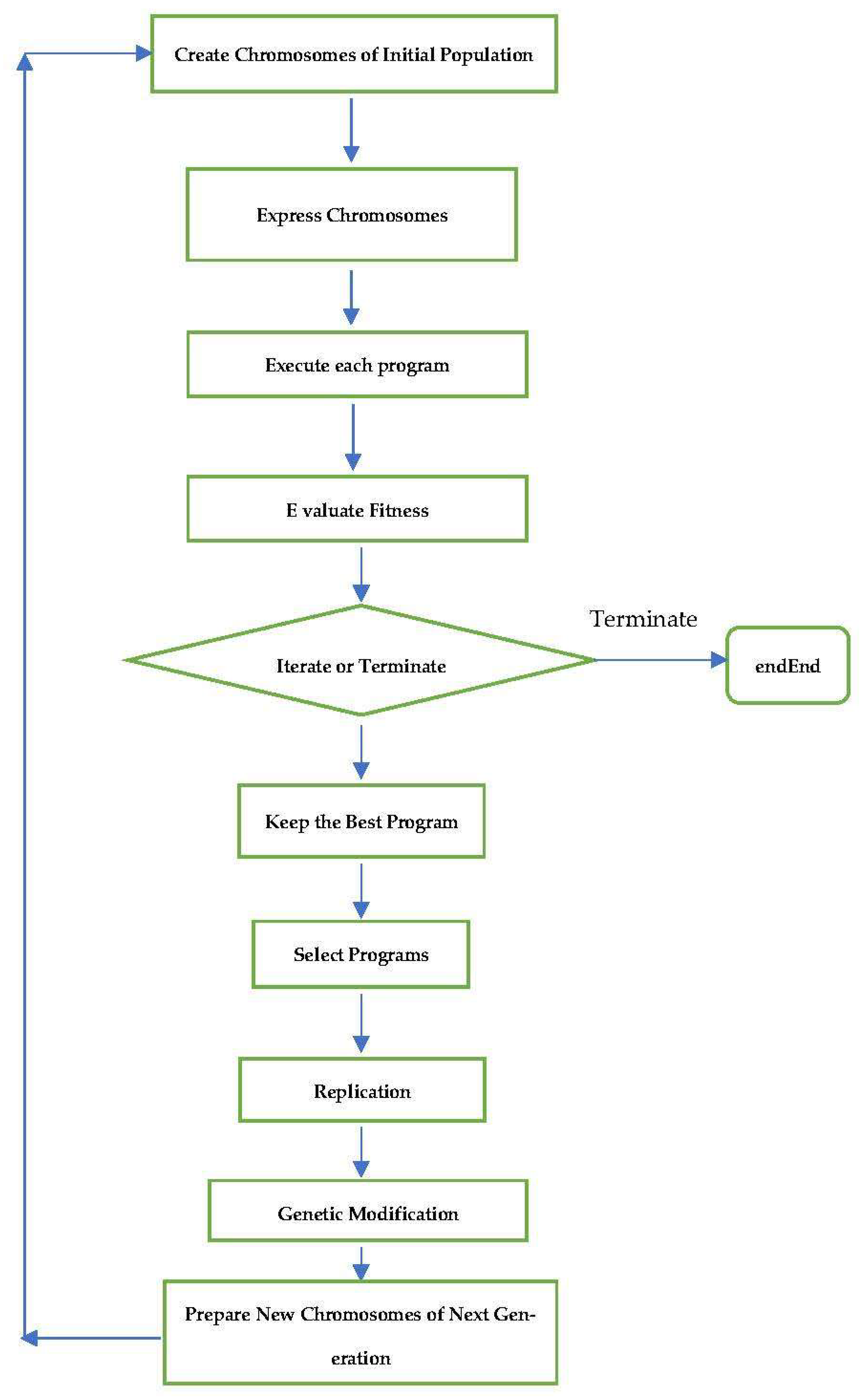
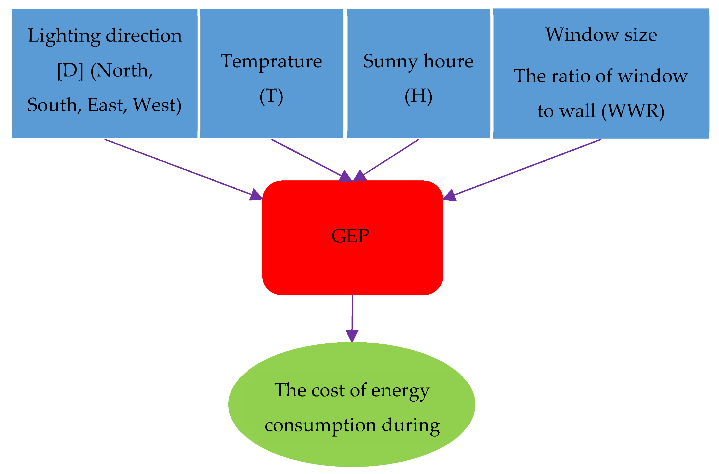
2.1. Development of a GEP Model

The GEP is an adaptive evolutionary algorithm that combines the best features of genetic algorithms (GA) with genetic programming (GP). After defining an objective function in the form of qualitative criteria, the aforementioned algorithms use this function to measure and compare various solution methods in a step-by-step process of correcting the data structure before selecting the most effective solution method, as presented. GEP is the most recent method among the circular algorithm methods, which are the most prevalent and widely used due to their sufficient precision. This method was developed relatively recently. With this distinction in mind, the genetic algorithm is the primary area of study in the programming of gene expression [29,30].

Head and tail domains comprise genes. The head domain has a function symbol and a term symbol, while the tail domain only has a term symbol. Users implementing GEP determine the head length, and Equation (1) calculates the tail length, as follows:

$$TL=HL\times \left(n-1\right)+1,$$

(1)

where TL and HL are the tail and head length, respectively, and n is the number of arguments for the function with the most arguments.

In this particular method, individual branches are utilized rather than bit strips. Each branch has its own unique collection of terminals, which represent the problem variables, and the total number of functions, which represent the main operators, is as follows:

• Selecting the terminal set, which consists of the same variables as the problem’s independent variables and the system’s state variables. This step involves the selection of the fit function, which typically employs the root-mean-square error (RMSE);
• Selecting a collection of functions, including mathematical operators, test functions, and Boolean functions;
• The model accuracy measurement index is used to determine the extent to which the model is capable of solving a specific problem;
• Control components, including the numerical component values and qualitative variables, are used to control the program’s execution;
• The number of data in the training section, the number of data in the test sections of the chromosomes, the size of the head, the number of genes, and the choice of the transplant operator, which can be adjusted with four options of addition, subtraction, multiplication, and division.

Equation (2) was used to analyze all produced chromosomes. GEP is finished if each program meets the termination criteria. The best software is kept.

$$\mathrm{Fitness} (i)={\sum }_{i=1}^m|CoE{\left(i\right)}_{\mathrm{act}}-CoE{\left(i\right)}_{\mathrm{for}}|,$$

(2)

where CoE(i)_act is the actual cost of energy, CoE(i)_for is the forecasted cost of energy using GEP or the optimized model, and m is the total number of data.

In this study, MATLAB was used to develop and implement genetic programming-based genes (see Appendix A). The structure of the GEP model is depicted in Figure 2. The procedure starts with the generation of chromosomes at random for a predetermined number of individuals or programs (the initial population). After this, the chromosomes are expressed, and the fitness of each program is compared to a collection of previously determined examples of fitness (also called the selection environment or training set). After that, the programs are selected in accordance with their finesses, which refers to their performance in that particular setting, in order to reproduce with modifications, thereby leaving children with new qualities. In turn, these new programs go through the same developmental process as the older ones, which includes chromosomal expression, confrontation with the selection environment, selection, and reproduction with alterations. The procedure is repeated until the desired result is achieved or for a predetermined number of generations, whichever comes first, as seen in Figure 2.

The GEP algorithm begins with the generation of the initial population of possible solutions as its first stage of execution. After this step, the chromosomes are expressed as a tree expression, which is then evaluated using a problem-fit function. This step can be accomplished through a random process or by making use of some prior information regarding the issue at hand. Processing a number of samples of the target problem, which are also referred to as fit cases, is commonly done in order to test the fit function in order to determine whether or not a solution is suitable for use within the parameters of the problem. The evolutionary process concludes when a satisfactory answer is discovered or when a predetermined number of generations has been reached. The report will then describe the optimal option. In the event that the stopping condition is not found, the most recent generation’s best solution will be preserved (assuming elite selection), and the remaining solutions will undergo a selection process. The survival function of merit plays a role in the selection process, and those with the highest merit have a greater chance of having children. This process is repeated for a number of generations in the hope that, on average, the quality of the population will improve as time passes. Using this method, a number of distinct occurrences are modified by employing a number of functions and terminals (

Table 2. Parameter values utilized in the GEP approach.

Genetic Functions		General Settings
Mutation rate	0.046	Chromosome number	32
Inversion rate	0.2	Vertex size	8
Insertion frequency	0.15	Number of genes per chromosome	4
Insertion rate	0.1	The number of productive populations	1150
Compounding single point	0.37

).

2.2. Optimization Method

In order to achieve the optimal combination of production units, determine their installation time and capacity in the GEP problem, and compare them, three different optimization algorithms have been performed in this study.

GSA is a meta-innovative optimization method based on Newton’s laws of gravitation and smooth contrast. GSAs are initialized with random objects scattered in the responsive space [31]. GSA has shown better performance in solving optimization problems compared to other algorithms [32]. Objects move as a result of the interaction between them by gravitational forces, which cause the general motion of objects towards heavier objects. Heavier objects exert more force on other objects and move slower than other objects. Objects considered in GSA are known based on their mass and the two vectors of velocity V and position ${\psi }_i$. Therefore, the ith object in the next N search space for i = 1, ..., L can be specified, as L shows the number of objects and $x_i^N$ shows the position of the ith object in the d dimension [33].

$${\psi }_i=\left[x_i^1,x_i^2,\dots ,x_i^N\right]$$

(3)

Improving GSA performance has been the goal of several studies. In this study, it is proposed to divide the search space, similar to parallel processing in the frog-leaping algorithm (SFL), and then use the strategy of considering the percentage of objects to calculate forces. Therefore, all the objects of group L, which includes μ in each group, are divided into objects. The objects of each group are responsible for a local search in the possible space. In each IGSA iteration, to classify objects, the performance indices of each object are calculated based on Equation (3), and then the objects are sorted incrementally based on their performance index values. Then, the first crime is assigned to the first group; the second crime is assigned to the second group, and so on. For each group, the motion of all objects is calculated [34]. Heavier objects in each group can be candidates for local minimum answers. To find a better answer to the internal interaction of objects in each group is considered. In the next step, a certain percentage of heavier objects is selected from each group, and the position of the objects is calculated based on the force exerted by these objects. Then, the best answer is selected, and to start the next step, all the objects are gathered together, and a new division is made for the possible space. This process continues until the convergence of the stop condition [35].

To use the GSA algorithms for the GEP problem, each chromosome/mass is defined by the vector M × 1, where M is the product of the number of steps (T_s) and the types of Candida (N)-generating units.

To optimize the GEP model, GSA is used, and then the best algorithm for solving the GEP problem by considering the fluctuations and uncertainty of wind production capacity in this study is selected. When the best algorithm is used to calculate the lower and upper ranges of a range and to cut a given alpha of each chromosome/mass, the TC value is calculated based on Equation (4) for each fuzzy number in each range. Then, the mean circuit of the TCs is determined as the bronze function in the optimization algorithm by considering the probability of each in the corresponding fuzzy number.

$$\mathrm{Fitness}={\sum }_{i=1}^K{\rho }_{i}T{C}_i,$$

(4)

where ${\rho }_i$ is the probability of the ith fuzzy number. Therefore, Equation (4) is used to determine the best fit or the best option in the issue of production development among the whole population [31].

3. Results and Discussion

In this section, the results of the developed model are presented. These results are related to the standard office room in Mumbai, India.

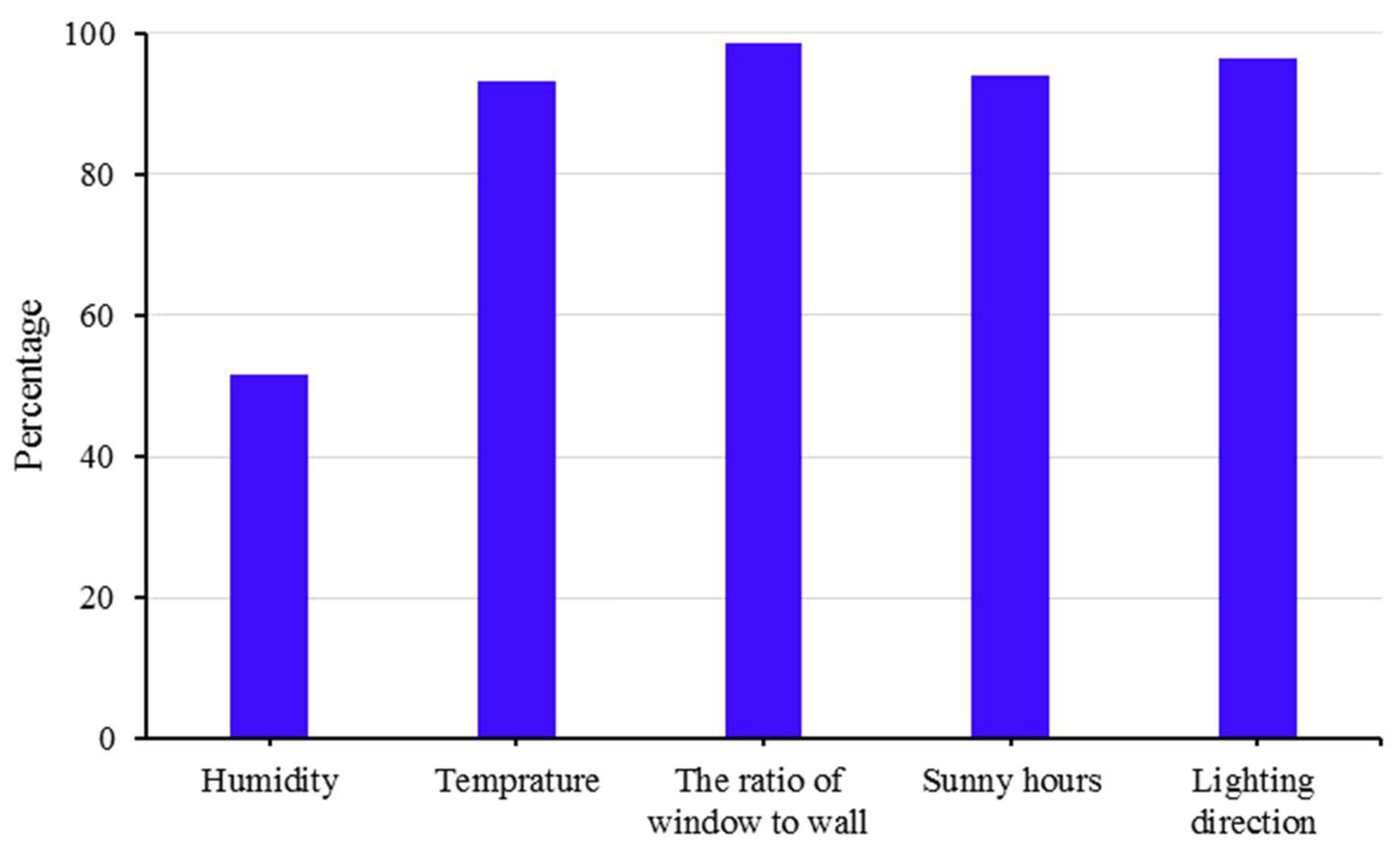
3.1. Sensitivity Analysis

There is a wide variety of methodologies available for carrying out sensitivity analyses in a wide variety of modeling and application settings. The existing modeling, as well as the type and nature of the data, will play a role in determining which approach will be taken to carry out this analysis. When it comes to conducting the aforementioned analysis, the one factor at a time (OFAT) method is one of the approaches that is considered to be among the most common and widespread. The procedure that is being described involves making a change to one of the model’s input variables while leaving the values of the other variables unchanged and then running the model. This procedure is carried out multiple times for each variable (parameter) until the influence of each parameter on the output has been analyzed and interpreted. This method is preferred by researchers over other sensitivity analysis methods in the majority of cases because of its high implementation and rationality stability. As a result, it is always able to produce favorable results and is preferred by researchers over other sensitivity analysis methods. In the event that the OFAT method fails (due to the fundamental nature of the model), it is simple to identify the effective parameter in the failure of the model, and by removing that factor from the calculations, the model’s robustness and the final accuracy of the analysis can be improved [36].

In the event that the OFAT method fails (due to the fundamental nature of the model), it is simple to identify the effective parameter in the failure of the model. In order to identify the power level and determine the effect of each of the parameters that were used in the study, it was necessary to first determine the power level. Comparisons were made for every factor that has the potential to influence energy consumption in order to evaluate the significance of each contributor to the overall result of the model. Figure 3 displays the findings of the sensitivity analysis that was performed. On the horizontal axis of this diagram are the parameters of the study, and on the vertical axis is a percentage representation of the effect that each of these parameters has on the model’s final output.

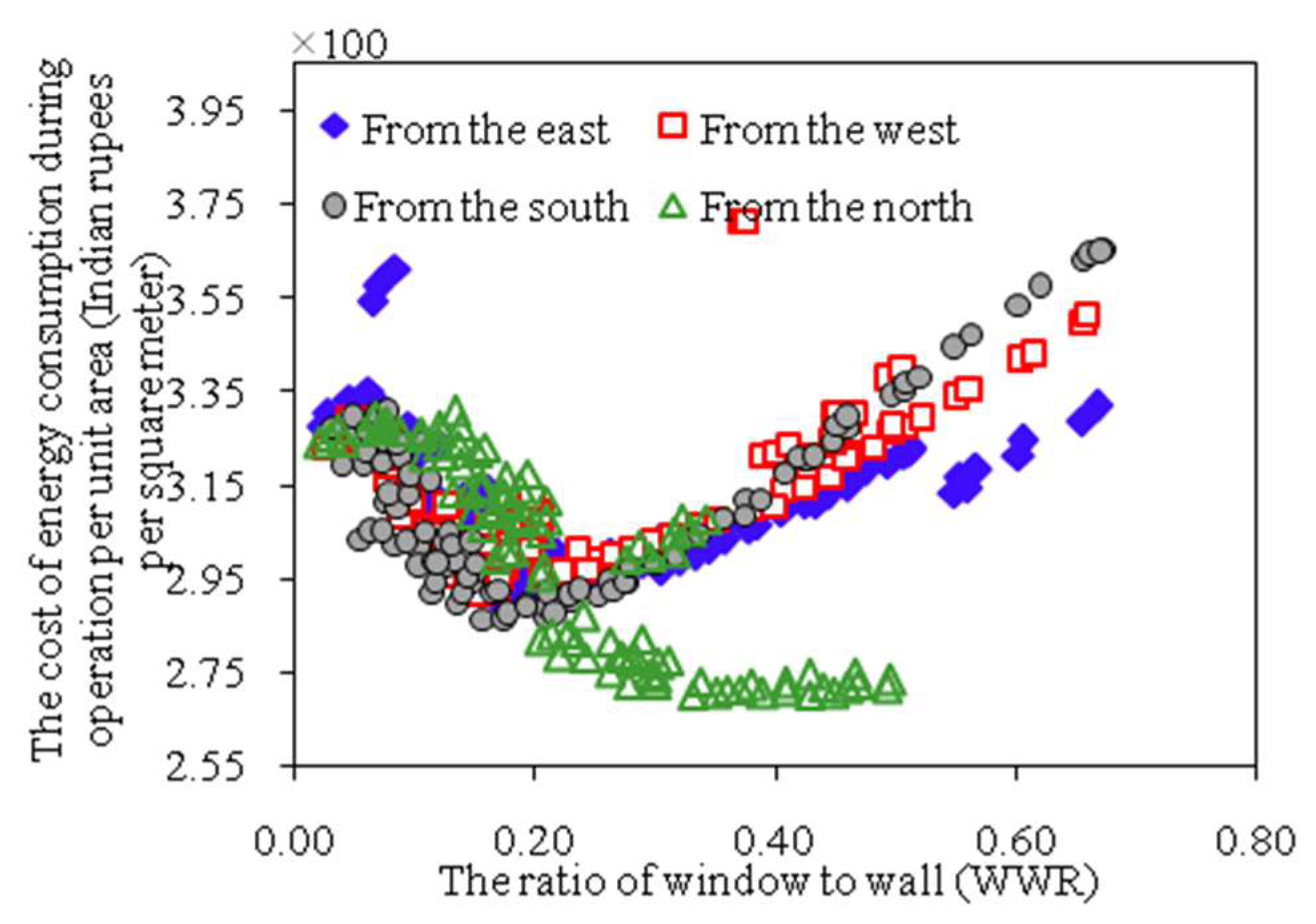
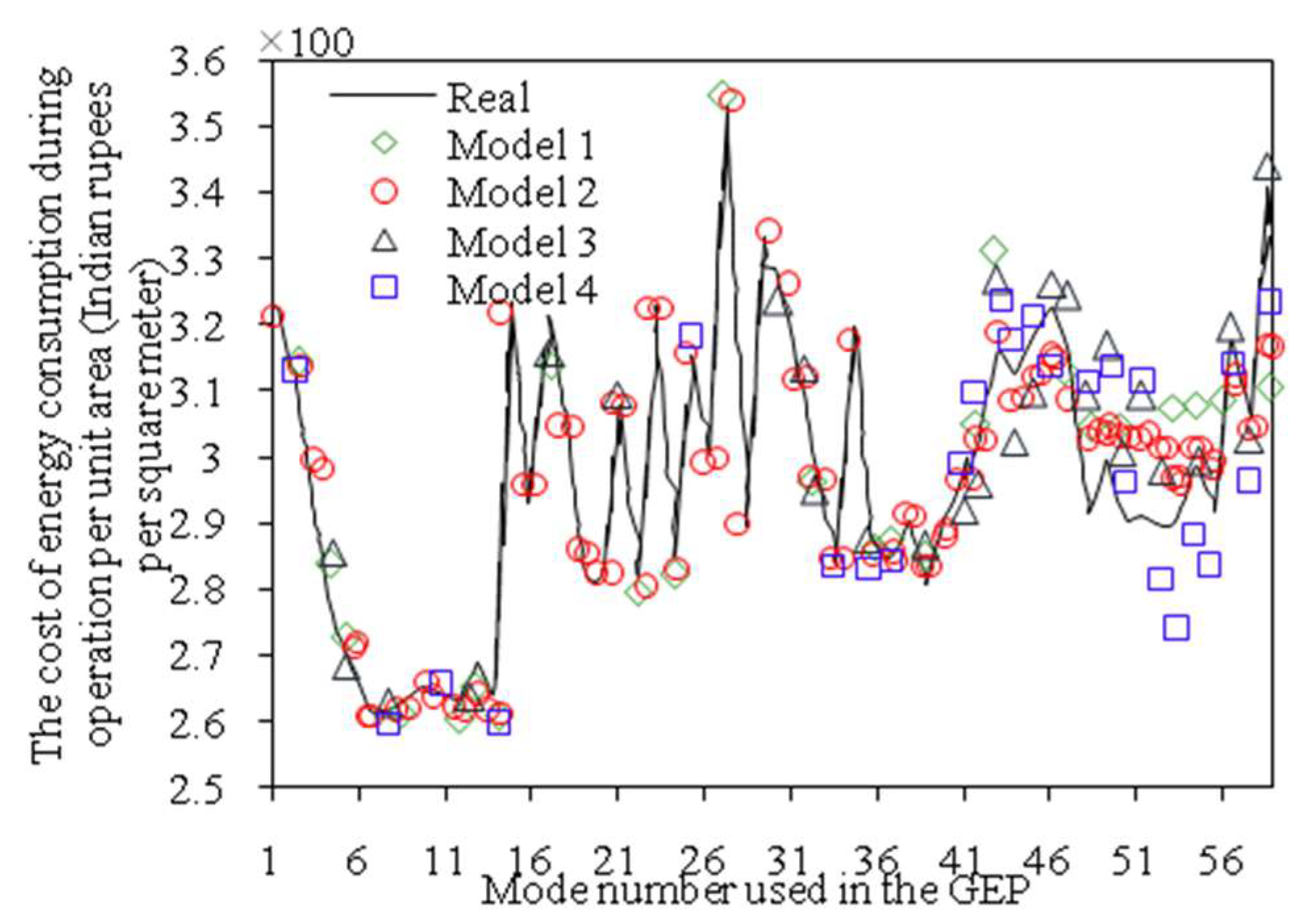
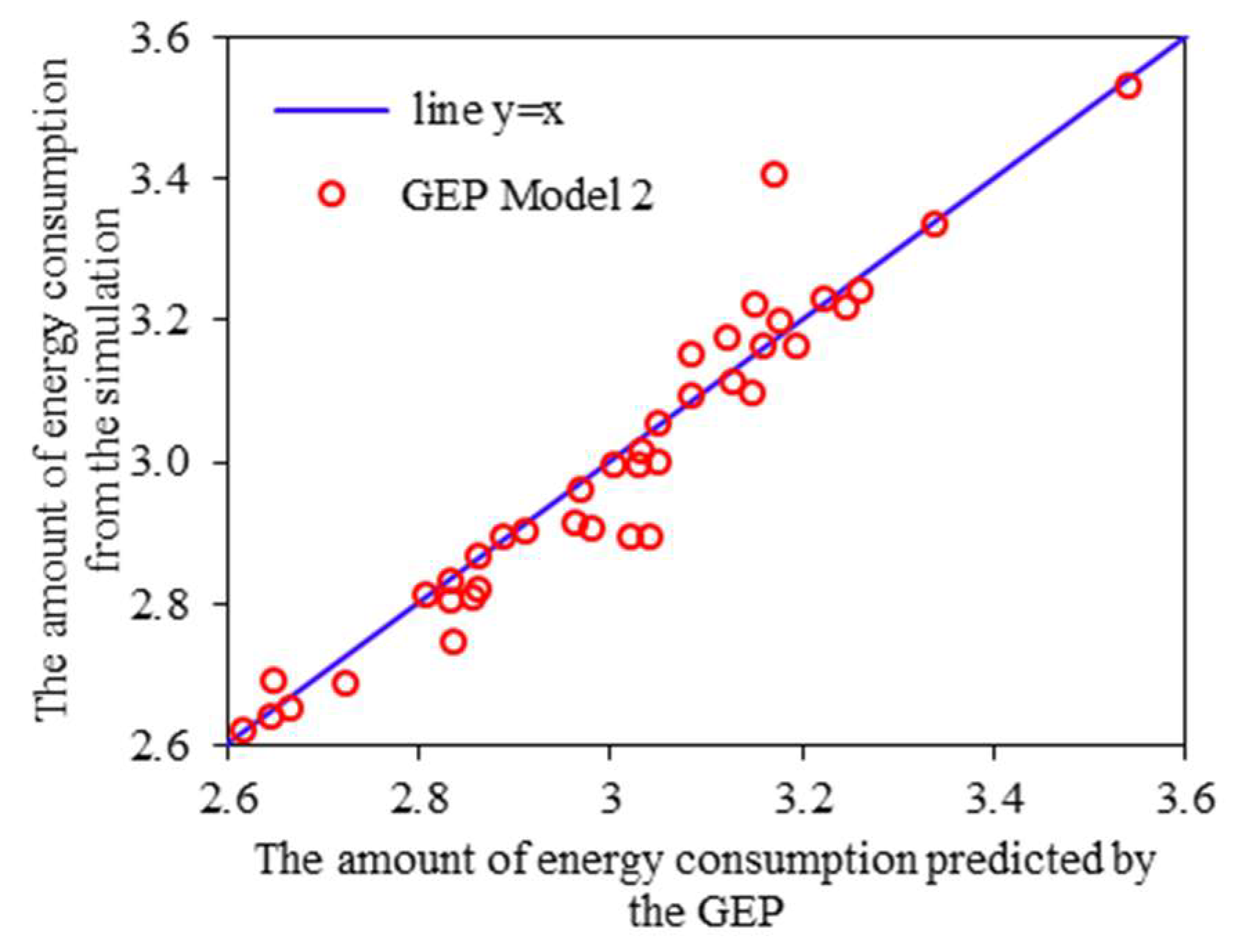
3.2. The Results of Model

The modeling was performed for a period of 20 years (the useful life of a course). In calculating the cost of gas and electricity, electricity and gas consumption tariffs of the Ministry of Energy and the standard room EnergyPlus model were used to model energy consumption. This model has been used for modeling a standard room in Mumbai by a researcher, and the accuracy of this model in estimating the consumption of electricity and gas with an error of about 6% has been proven. During a preliminary study, it was found that the components for lighting and the dimensions of the selected window for the standard room have a significant effect on the amount of electricity and gasoline used. Energy consumption costs during operations were obtained from the total cost of gas and electricity consumption during operations, which is shown in Figure 4.

As mentioned, 380 modeling modes were generated for the standard room under consideration by changing the direction of lighting and the ratio of the window surface to the wall, and in each case, the amount of electricity and gas consumption per unit area was calculated and determined as the cost of energy consumption.

During the operation of the office room, GEP tools were utilized in order to facilitate the forecasting of the costs associated with the room’s energy consumption. This was carried out in order to facilitate the forecasting of the costs associated with energy consumption. The implementation of an energy consumption simulation model for architectural engineers is a time-consuming design for an office room that requires various types of training. It is possible to make an accurate prediction of the costs associated with the building’s construction and operation in relation to the scenario that has been selected by selecting the proportions of the window and the lighting direction. Because it was determined that the cost of energy consumption during the operation of the room is dependent on the percentage of the window and the direction of lighting based on the sensitization that was performed in the numerical modeling section, the structure of the GEP that was developed is consistent with the structure that is shown in Figure 5. This is because it was determined that the cost of energy consumption during the operation of the room depends on the direction of lighting. To test the network, a random 21% of the data from the results of 288 different simulation modes were taken out of the simulated case set and used. In total, this represents approximately 21% of the data. When choosing the data that would be used for the test, it was done in such a way that 15 different pieces would be chosen at random to be removed from each exposure direction. This was done so that the results would be more accurate. The last of the data were put to use in the process of training neural networks to function according to GEP. The performance of a number of models on test data was evaluated using the criteria of the correlation coefficient, mean error squared, mean normalized error squared, and root-mean-square error, and at the end of the process, the most intelligent model with the best performance was suggested as the model to use.

Four types of GEP models based on the sensitivity analysis were utilized in this study. Due to its chromosomal syntax, GEP is comparable to GA and genetic programming. They were chosen with consideration for their adaptability, and genetic transformation was then accomplished with the aid of genetic operators. Due to the increasing use of GEP, a variety of software is available, the most popular and widely used of which is neural network software written in the MATLAB programming language. The MATLAB tool was created by multiple researchers and employs multiple methods to train the GEP. The functions used to teach the network are displayed in

Table 3. Design Combination.

Model ID	Input Variables
Design Combo 1 (D1)	Dt, Tt−1, WWRt
Design Combo 2 (D2)	Dt, Tt−3, Ht−1, WWRt
Design Combo 3 (D3)	Dt, Tt−1, Ht−1, WWRt
Design Combo 4 (D4)	Dt, Tt−2, Tt−3, Ht−2, Ht−1, WWRt

.

As shown in

Table 4. Performance of GEP models.

Model ID	MAE	RMSE	R	MAE	RMSE	R
	Training			Testing
D1	0.01818	0.14567	0.88776	0.01920	0.14567	0.86528
D2	0.01631	0.089646	0.92956	0.01812	0.09146	0.90825
D3	0.01762	0.09220	0.90319	0.01895	0.10220	0.88526
D4	0.01925	0.12134	0.91351	0.01735	0.12134	0.89543

, the existing algorithms for training are extremely diverse, and previous research has demonstrated that none of them is applicable in every situation. In this study, all MATLAB toolbox functions were utilized to determine the training algorithm that produces the least amount of error in the training data for a variety of different models.

A number of network training modes were executed, and the mode with the lowest RMSE and highest correlation coefficient was selected. This was achieved by retaining the examination of the various models of GEP program adjustment factors for every number of orientations and then executing the training modes. As shown in the table, the Model 2 GEP (D2), which corresponds to the least amount of error, can be considered the best answer. Figure 6 also displays the results of comparing the predicted values to the actual values (based on the energy simulator model) to determine the most effective model.

As can be seen, the accuracy of the predictions for the west is lower compared to those for the other directions, and the predictions that correspond to light coming from the south are the ones that are the most accurate. Figure 6 depicts a distribution diagram of energy consumption values during operations per unit area obtained from the use of trained GEP versus observational values based on an energy consumption simulation model for test data. This was done in order to evaluate the performance of the best-trained neural network. Figure 7 demonstrates that the trained GEP is functioning properly, and in fact, the network has been able to make accurate predictions.

4. Conclusions

In this particular piece of research, a novel approach that forecasts standard energy usage and is founded on GEP has been presented. In this approach, the rule of physics that underlies the problem is determined, as well as the relationship between the inputs and outputs of the system, with the assistance of data on the system’s inputs and outputs that were collected via a simulation of normal energy consumption. This technology eliminates the requirement for simulation, which results in both a fast rate of speed and a high level of accuracy. This method requires the execution of a number of simulations at the outset so that the simulation results can be used to train the GEP. After that, the trained network assumes the role of the simulated model, and it is no longer necessary to implement a simulation model in order to predict the amount of energy consumed. The trained network then replaces the simulated model, making energy consumption predictable without the need to implement a simulation model. To evaluate the performance of the proposed structure, a standard office room was modeled for 380 different lighting scenarios to determine energy consumption using the EnergyPlus tool in order to obtain the required database for GEP training. Statistical indicators were then used to evaluate the performance of the trained network based on these models. According to the evaluation results, the range of changes in the MAE is between 0.01735 and 0.01920.

The lack of precise design criteria for the optimal use of energy in office spaces, combined with the significant contribution that office spaces make to the overall energy consumption of urban areas, means that office area designers can avoid expensive and time-consuming energy consumption simulation calculations by providing geometric specifications and a location that takes into account an intelligent system. In order to accomplish this objective, a comparison of four GEP models was carried out, with 80% of the data being used for training and 20% being used for testing. The gravitational search algorithm (GSA) was utilized in order to achieve the best possible results from the model. Using the suggested framework, the architect may quickly determine the energy consumption of a variety of lighting options and make a decision regarding the window design choice that would result in the lowest energy consumption. The proposed new tool makes it possible for the architect to quickly compare the various options for lighting an office room in terms of energy consumption and to select the best option that corresponds to the lowest energy cost. Since the results of the present study are limited to the dimensions of a standard office room in a particular climate, future studies can focus on the effect of climate, office room dimensions, and other components defining architectural space on energy consumption.

The data range that was used for the models’ calibration imposes limitations on the extent to which they are capable of making accurate predictions. Despite the fact that this limitation exists, the models can be readily retrained and improved so that they can make more accurate predictions across a wider range of scenarios by incorporating data from other case studies.

References

1. Pilechiha, P.; Mahdavinejad, M.; Pour Rahimian, F.; Carnemolla, P.; Seyedzadeh, S. Multi-Objective Optimisation Framework for Designing Office Windows: Quality of View, Daylight and Energy Efficiency. Appl. Energy 2020, 261, 114356. [Google Scholar] [CrossRef]
2. Sadick, A.-M.; Kamardeen, I. Enhancing Employees’ Performance and Well-Being with Nature Exposure Embedded Office Workplace Design. J. Build. Eng. 2020, 32, 101789. [Google Scholar] [CrossRef]
3. Anand, P.; Cheong, D.; Sekhar, C.; Santamouris, M.; Kondepudi, S. Energy Saving Estimation for Plug and Lighting Load Using Occupancy Analysis. Renew. Energy 2019, 143, 1143–1161. [Google Scholar] [CrossRef]
4. Ahmadi, M.H.; Ghazvini, M.; Sadeghzadeh, M.; Alhuyi Nazari, M.; Kumar, R.; Naeimi, A.; Ming, T. Solar Power Technology for Electricity Generation: A Critical Review. Energy Sci. Eng. 2018, 6, 340–361. [Google Scholar] [CrossRef] [Green Version]
5. Azizi, H.; Nejatian, N. Evaluation of the Climate Change Impact on the Intensity and Return Period for Drought Indices of SPI and SPEI (Study Area: Varamin Plain). Water Supply 2022, 22, 4373–4386. [Google Scholar] [CrossRef]
6. Yavari, F.; Salehi Neyshabouri, S.A.; Yazdi, J.; Molajou, A.; Brysiewicz, A. A Novel Framework for Urban Flood Damage Assessment. Water Resour. Manag. 2022, 36, 1991–2011. [Google Scholar] [CrossRef]
7. Karimi, G.; Moradi, Y. Buffer Insertion for Delay Minimization in RLC Interconnects Using Cuckoo Optimization Algorithm. Analog Integr. Circuits Signal Process. 2019, 99, 111–121. [Google Scholar] [CrossRef]
8. Omrani, M.M. Techno-Economic and Environmental Analysis of Floating Photovoltaic Techno-Economic and Environmental Analysis of Floating Photovoltaic Power Plants: A Case Study of Iran. Renew. Energy Res. Appl. 2022, 4, 41–54. [Google Scholar] [CrossRef]
9. Jalali, Z.; Noorzai, E.; Heidari, S. Design and Optimization of Form and Facade of an Office Building Using the Genetic Algorithm. Sci. Technol. Built Environ. 2020, 26, 128–140. [Google Scholar] [CrossRef]
10. O’Brien, W.; Wagner, A.; Schweiker, M.; Mahdavi, A.; Day, J.; Kjærgaard, M.B.; Carlucci, S.; Dong, B.; Tahmasebi, F.; Yan, D.; et al. Introducing IEA EBC Annex 79: Key Challenges and Opportunities in the Field of Occupant-Centric Building Design and Operation. Build. Environ. 2020, 178, 106738. [Google Scholar] [CrossRef]
11. Elsheikh, A.H.; Shanmugan, S.; Sathyamurthy, R.; Kumar Thakur, A.; Issa, M.; Panchal, H.; Muthuramalingam, T.; Kumar, R.; Sharifpur, M. Low-Cost Bilayered Structure for Improving the Performance of Solar Stills: Performance/Cost Analysis and Water Yield Prediction Using Machine Learning. Sustain. Energy Technol. Assess. 2022, 49, 101783. [Google Scholar] [CrossRef]
12. Ahmadi, M.H.; Baghban, A.; Salwana, E.; Sadeghzadeh, M.; Zamen, M.; Shamshirband, S.; Kumar, R. Machine Learning Prediction Models of Electrical Efficiency of Photovoltaic-Thermal Collectors. Preprints 2019, 2019050033. [Google Scholar] [CrossRef] [Green Version]
13. Sabbagh, O.; Fanaei, M.A.; Arjomand, A.; Hossein Ahmadi, M. Multi-Objective Optimization Assessment of a New Integrated Scheme for Co-Production of Natural Gas Liquids and Liquefied Natural Gas. Sustain. Energy Technol. Assess. 2021, 47, 101493. [Google Scholar] [CrossRef]
14. Gielen, D.; Boshell, F.; Saygin, D.; Bazilian, M.D.; Wagner, N.; Gorini, R. The Role of Renewable Energy in the Global Energy Transformation. Energy Strategy Rev. 2019, 24, 38–50. [Google Scholar] [CrossRef]
15. Ahmadi, M.H.; Açıkkalp, E. Exergetic Dimensions of Energy Systems and Processes. J. Therm. Anal. Calorim. 2021, 145, 631–634. [Google Scholar] [CrossRef]
16. Lowitzsch, J.; Hoicka, C.E.; van Tulder, F.J. Renewable Energy Communities under the 2019 European Clean Energy Package—Governance Model for the Energy Clusters of the Future? Renew. Sustain. Energy Rev. 2020, 122, 109489. [Google Scholar] [CrossRef]
17. Fessler, D.C. The Energy Disruption Triangle: Three Sectors That Will Change How We Generate, Use, and Store Energy; Wiley: Hoboken, NJ, USA, 2018; ISBN 9781119347132. [Google Scholar]
18. Li, Q.; Loy-Benitez, J.; Nam, K.; Hwangbo, S.; Rashidi, J.; Yoo, C. Sustainable and Reliable Design of Reverse Osmosis Desalination with Hybrid Renewable Energy Systems through Supply Chain Forecasting Using Recurrent Neural Networks. Energy 2019, 178, 277–292. [Google Scholar] [CrossRef]
19. Sudharshan, K.; Naveen, C.; Vishnuram, P.; Krishna Rao Kasagani, D.V.S.; Nastasi, B. Systematic Review on Impact of Different Irradiance Forecasting Techniques for Solar Energy Prediction. Energies 2022, 15, 6267. [Google Scholar] [CrossRef]
20. Davoodi, A.; Abbasi, A.R.; Nejatian, S. Multi-Objective Techno-Economic Generation Expansion Planning to Increase the Penetration of Distributed Generation Resources Based on Demand Response Algorithms. Int. J. Electr. Power Energy Syst. 2022, 138, 107923. [Google Scholar] [CrossRef]
21. Dagoumas, A.S.; Koltsaklis, N.E. Review of Models for Integrating Renewable Energy in the Generation Expansion Planning. Appl. Energy 2019, 242, 1573–1587. [Google Scholar] [CrossRef]
22. Taherkhani, M.; Hosseini, S.H.; Javadi, M.S.; Catalão, J.P.S. Scenario-Based Probabilistic Multi-Stage Optimization for Transmission Expansion Planning Incorporating Wind Generation Integration. Electr. Power Syst. Res. 2020, 189, 106601. [Google Scholar] [CrossRef]
23. Pokhrel, S.; Amiri, L.; Zueter, A.; Poncet, S.; Hassani, F.P.; Sasmito, A.P.; Ghoreishi-Madiseh, S.A. Thermal Performance Evaluation of Integrated Solar-Geothermal System; a Semi-Conjugate Reduced Order Numerical Model. Appl. Energy 2021, 303, 117676. [Google Scholar] [CrossRef]
24. Paliwal, P.; Webber, J.L.; Mehbodniya, A.; Haq, M.A.; Kumar, A.; Chaurasiya, P.K. Multi-Agent-Based Approach for Generation Expansion Planning in Isolated Micro-Grid with Renewable Energy Sources and Battery Storage. J. Supercomput. 2022, 78, 18497–18523. [Google Scholar] [CrossRef]
25. Sweerts, B.; Pfenninger, S.; Yang, S.; Folini, D.; van der Zwaan, B.; Wild, M. Estimation of Losses in Solar Energy Production from Air Pollution in China since 1960 Using Surface Radiation Data. Nat. Energy 2019, 4, 657–663. [Google Scholar] [CrossRef]
26. Azimi, H.; Bonakdari, H.; Ebtehaj, I. Gene Expression Programming-Based Approach for Predicting the Roller Length of a Hydraulic Jump on a Rough Bed. ISH J. Hydraul. Eng. 2021, 27, 77–87. [Google Scholar] [CrossRef]
27. Pirzadeh Ashraf, B.; Mojtahedi, A.; Dadashzadeh, M. Prediction of dissolved oxygen in wetlands using FCM-ANFIS model—A Case Study: Choghakhor Wetland. J. Iran. Water Eng. Res. 2022, 2, 33–50. [Google Scholar] [CrossRef]
28. Han, T.; Ansari, N. Provisioning Green Energy for Base Stations in Heterogeneous Networks. IEEE Trans. Veh. Technol. 2016, 65, 5439–5448. [Google Scholar] [CrossRef] [Green Version]
29. Drachal, K.; Pawłowski, M. A Review of the Applications of Genetic Algorithms to Forecasting Prices of Commodities. Economies 2021, 9, 6. [Google Scholar] [CrossRef]
30. Tijani, I.A.; Zayed, T. Gene Expression Programming Based Mathematical Modeling for Leak Detection of Water Distribution Networks. Measurement 2022, 188, 110611. [Google Scholar] [CrossRef]
31. Mittal, H.; Tripathi, A.; Pandey, A.C.; Pal, R. Gravitational Search Algorithm: A Comprehensive Analysis of Recent Variants. Multimed. Tools Appl. 2021, 80, 7581–7608. [Google Scholar] [CrossRef]
32. Sabri, N.M.; Puteh, M.; Mahmood, M.R. An Overview of Gravitational Search Algorithm Utilization in Optimization Problems. In Proceedings of the 2013 IEEE 3rd International Conference on System Engineering and Technology, Shah Alam, Malaysia, 19–20 August 2013; pp. 61–66. [Google Scholar]
33. Wang, Y.; Gao, S.; Yu, Y.; Cai, Z.; Wang, Z. A Gravitational Search Algorithm with Hierarchy and Distributed Framework. Knowl. -Based Syst. 2021, 218, 106877. [Google Scholar] [CrossRef]
34. Rashedi, E.; Rashedi, E.; Nezamabadi-pour, H. A Comprehensive Survey on Gravitational Search Algorithm. Swarm Evol. Comput. 2018, 41, 141–158. [Google Scholar] [CrossRef]
35. Younes, Z.; Alhamrouni, I.; Mekhilef, S.; Reyasudin, M. A Memory-Based Gravitational Search Algorithm for Solving Economic Dispatch Problem in Micro-Grid. Ain Shams Eng. J. 2021, 12, 1985–1994. [Google Scholar] [CrossRef]
36. Campbell, J.E.; Carmichael, G.R.; Chai, T.; Mena-Carrasco, M.; Tang, Y.; Blake, D.R.; Blake, N.J.; Vay, S.A.; Collatz, G.J.; Baker, I.; et al. Photosynthetic Control of Atmospheric Carbonyl Sulfide during the Growing Season. Science 2008, 322, 1085–1088. [Google Scholar] [CrossRef]
Figure 1. The plan of a standard office room.
Sustainability 15 01728 g001
Figure 2. The fundamental steps of GEP are schematically represented in the flowchart.
Sustainability 15 01728 g002
Figure 3. Robust rate of the model against each of the parameters.
Sustainability 15 01728 g003
Figure 4. Energy consumption cost during the operation of the standard office room in Mumbai.
Sustainability 15 01728 g004
Figure 5. Inputs and outputs of the GEP structure developed in this study.
Sustainability 15 01728 g005
Figure 6. Comparative diagram of the validation results of the best GEP obtained for a number of different models.
Sustainability 15 01728 g006
Figure 7. Comparative diagram of the validation result of the best GEP trained in predicting energy consumption during operations per unit area (million rails per square meter).
Sustainability 15 01728 g007