Energy Consumption and Carbon Dioxide Production Optimization in an Educational Building Using the Supported Vector Machine and Ant Colony System

Abstract

Buildings account for sixty percent of the world’s total annual energy consumption; therefore, it is essential to find ways to reduce the amount of energy used in this sector. The road administration organization in Jakarta, Indonesia, utilized a questionnaire as well as the insights of industry experts to determine the most effective energy optimization parameters. It was decided to select variables such as the wall and ceiling materials, the number and type of windows, and the wall and ceiling insulation thickness. Several different modes were evaluated using the DesignBuilder software. Training the data with a supported vector machine (SVM) revealed the relationship between the inputs and the two critical outputs, namely the amount of energy consumption and CO₂ production, and the ant colony algorithm was used for optimization. According to the findings, the ratio of the north and east windows to the wall in one direction is 70 percent, while the ratio of the south window to the wall in the same direction ranges from 35 to 50 percent. When the ratio and percentage of the west window to the west wall is between 60 and 70 percent, the amount of produced energy and CO₂ is reduced to negligible levels.

1. Introduction

Energy consumption in buildings accounts for 60% of the world’s annual energy consumption and 43% of the world’s greenhouse gas emission [1,2,3,4]. Emissions of greenhouse gases, particularly CO₂, have a significant impact on both climate change and the warming of the planet [5]. Climate change and global warming cause many challenges to the world such as increases in urban floods [6,7,8]. The first step towards achieving smart buildings is energy consumption analysis and optimization. The growth of electric energy consumption and its dependence on polluting fossil fuels, especially in domestic and commercial uses, has led researchers to think of ways to control the amount of energy consumption in buildings [9]. Therefore, it is very important to provide solutions that can reduce energy consumption in this sector [10]. Compliance with the smallest details can have a great impact on reducing energy consumption in buildings; for example, the way the building is oriented, the way the side spaces are located, and the improvement of insulation methods with the lowest cost can improve the energy efficiency of buildings, and thus by correcting the construction methods building design can achieve ideal design [11,12,13].

Most of the parameters of a building, including the thermal conductivity of the walls, the air permeability, the number of occupants, and the consumption of heating and cooling devices, are uncertain in nature, because they depend on changes in the weather and the behavior of the residents [14,15]. Saving energy consumption by paying attention to the placement of spaces in the plan based on matching the pattern of space occupation with the solar cycle, choosing the shell suitable for the climate and environmental conditions, setting the dimensions of the opening according to the received radiation and heat loss resulting from it, as well as the types of opening and glass are effective in reducing building energy consumption [16]. Carrying out proper planning in the field of energy consumption and management in smart educational buildings has made it possible to reduce more than 30% of annual energy consumption [17]. A multi-objective optimization method determines the building’s exterior insulation thickness based on environmental and economic factors. Buildings with white or near-white exteriors, medium-capacity and thermal-resistant building materials, and tiny windows with awnings have lower inside air temperatures throughout the day [18]. However, buildings with dark exterior walls or large windows without awnings will have warmer indoor air than outside air during the day. Therefore, the importance of ventilation in changing the indoor air of a building depends on the external surface of its walls, as well as the size of the windows and the quality of the canopy. Using optimization, a multi-objective optimization model is presented to improve building energy performance [12].

In recent decades, machine learning methods have been used to model many scientific problems, and the results obtained from these methods have a significant compatibility with the measured values in the scale of real data [13,19,20,21]. The Support Vector Machine (SVM) method is also one of the machine learning methods that was introduced in the 1990s [12,13,18]. Despite the fact that the SVM method is a relatively new method, its wide use in the modeling of phenomena has been established and the results have been satisfactory [22,23].

In this study, the SVM method was used to predict the energy consumption of educational facilities. This article’s primary objectives are to present and develop a reliable model for predicting building energy consumption using the SVM method and to optimize the effective parameter in energy usage in educational buildings using the ant colony system (ACS). First, the building’s effective parameters are evaluated. Effective parameters are parameters whose value changes have noticeable effects on the energy consumption of the building. Then, an educational building in Jakarta, Indonesia is modeled using DesignBuilder (V5.5.2.007) tools and the effect of these parameters on the building’s energy consumption and CO₂ is studied. As input data for the soft computing and optimization method, the building’s physical characteristics, such as the window-to-wall ratio, were evaluated. By examining this topic, we attempt to answer the question of how the physical characteristics of a school building affect energy consumption and CO₂ emissions.

2. Materials and Methods

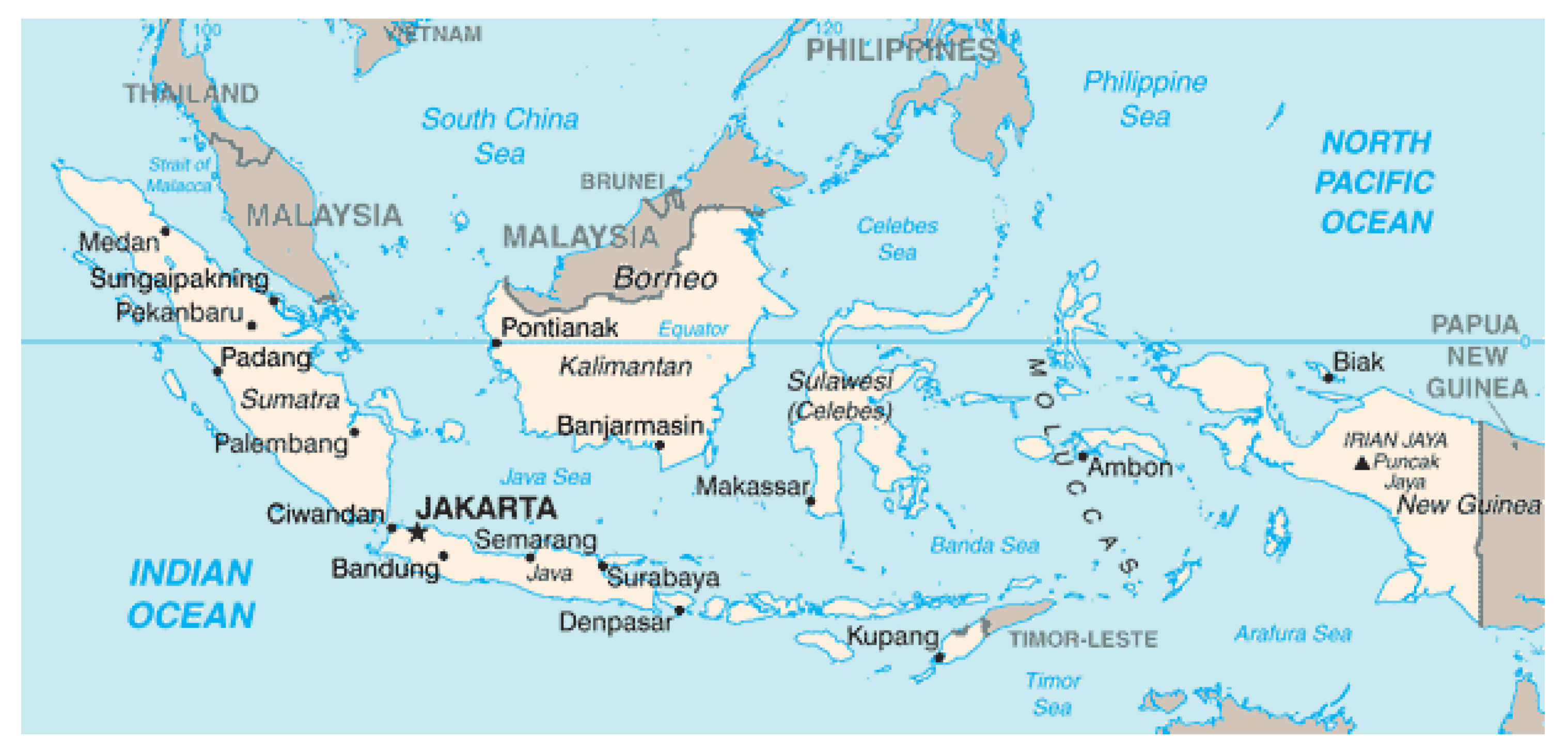
2.1. Case Study

This study chose the road administration organization building in Jakarta as a case study (Figure 1). The environmental data for modeling are related to Jakarta, Indonesia. A summary of Jakarta’s climate conditions is presented in

Table 1. Summary of climate conditions in Jakarta.

Annual Values	Jakarta, Sumatra, Indonesia
Daytime maximum temperature	31.70 °C
Daily low temperature	23.60 °C
Water temperature	28.20 °C
Humidity	83%
Precipitation	2584 mm
Rain days	152.4 days
Hours of sunshine	1789 h

. In the present study an educational building in Jakarta was modelled based on these environmental conditions.

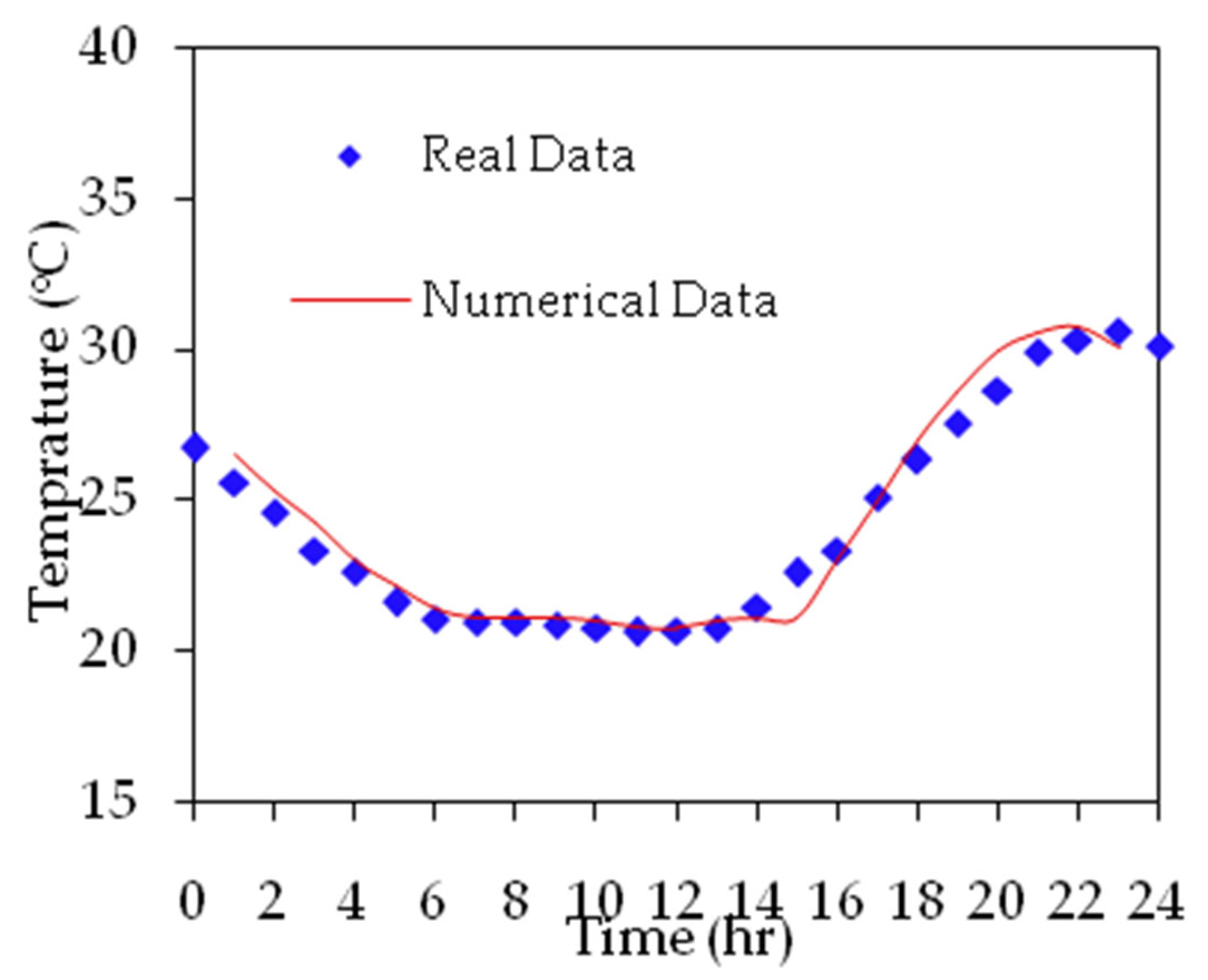
2.2. DesignBuilder Model Validation

To validate the model of the educational building according to Figure 2, it was simulated in DesignBuilder.

The temperature of a classroom was evaluated in order to validate the model. It is assumed in the models that the surrounding air has a constant temperature (by the heat guard). Establishing the conditions is the initial step in the procedure for validating the DesignBuilder results. This is relevant for DesignBuilder’s adaptation of the associated graphs of practical testing and simulation. According to the RMSE, the statistical analysis of the numerical and experimental results of temperature reveals that the model’s performance is satisfactory (RMSE = 1.08). In capturing the experiments accurately, the models meet all objectives (Figure 3).

To minimize energy usage and greenhouse gases emissions for low-energy buildings, it is required to first examine the desired building’s existing energy consumption and then compare it with the numerical results. For this purpose, monthly electricity bills for the building in 2020 were created and adjusted for comparison with the numerical data.

The hottest months of the year (June and July) have the highest electricity consumption, while the peak electricity load is 409,555 kilowatt hours and the lowest electricity demand is 49,868 kilowatt hours, according to studies regarding electricity bills.

In the existing state, the wall material is brick, the roof material is beam, the cooling system is split, and the window is made of wood with double-glazed glass. The aforementioned data were entered into the DesignBuilder software, and the heat transfer coefficient for each building component was calculated. To simulate and enter the details, the software’s information was utilized. The details of the roof and wall of the desired building in DesignBuilder before optimization are shown in

Table 2. Characteristics regarding the materials utilized for the existing and optimal ceiling and interior and exterior walls.

Building Elements	Materials	Heat Transfer Coefficient (W/m2.k)	Thickness (mm)
Existing
Reinforced concrete girder	Mosaic	1.456	22
	Plaster		45
	Waterproofing		45
	Concrete		105
	Block		250
	Plaster		45
Brick wall		2.650	220
Optimal
Concrete Slab	Bituminous waterproofing	1.520	32
	Plaster		25
	Lightweight concrete		40
	Concrete		250
	Plaster		20
Concrete wall	Lightweight concrete	2.291	125
	Plaster		22
Roof insulation	Polystyrene	0.750	35
	Polystyrene	0.645	40
Wall insulation	Polystyrene	0.844	35
	Polystyrene	0.541	40
Double-glazed glass	Two layers of glass	1.562	8
	Argon gas Two layers of		3
Window triple glass	transparent glass	0.656	4
	Low emissivity glass		1
	Krypton gas		15

. In this situation, the heat transmission coefficient of the roof is 1.456 W/m²k. The materials utilized in the construction of the external-to-interior brick wall are exterior brick and plaster and the heat transfer coefficient of the wall in this instance is 2.650 W/m²k.

Various energy-optimization techniques have been offered to minimize the building’s energy consumption, including optimizing the window-to-wall ratio, wall and ceiling insulation, employing triple-glazed windows, and utilizing varied roof and wall detailing. In each optimization solution, the amount of cooling load reduction is computed, and the best state is then simulated by merging these solutions. In addition, Table 2 displays the roof and wall features of the intended structure in the DesignBuilder software’s optimal mode. In the optimal mode, the materials used in the concrete slab roof are, from top to bottom, plaster, light concrete, and concrete; in this instance, the heat transfer coefficient of the roof is 1.520 W/m²k. The materials utilized in the concrete wall from the exterior to the interior of the building are light concrete and plaster and the heat transfer coefficient of the wall in this instance is 2.291 W/m²k.

The use of a brick wall compared to a concrete wall, a beam roof compared to a concrete slab roof, triple-paned glass compared to double-paned glass, the use of 40 mm polystyrene insulation compared to 35 mm insulation in a brick wall were investigated. In addition, the beam roof reduces the amount of cooling energy of the building and reduces the heat loss of the building.

All of the facts about the building, which was identified as successful in energy optimization in the previous section, are entered into this part of the software, and the software optimizes based on the least amount of energy consumed and the least amount of CO₂ emitted. The key element in this section is that the brick wall is compared to the concrete wall, the beam ceiling is compared to the concrete slab, triple- and double-glazed glass is compared to regular glass, and wall and ceiling insulation is 40 mm thick in optimization. The building energy is effective and generates reduced energy loss; therefore, it has been added as an effective choice in the DesignBuilder optimization. The window-to-wall percentages on the north, south, east, and west fronts, on the other hand, are defined as 15, 20, 45, and 60 percent, and the output of this component includes the total energy and CO₂.

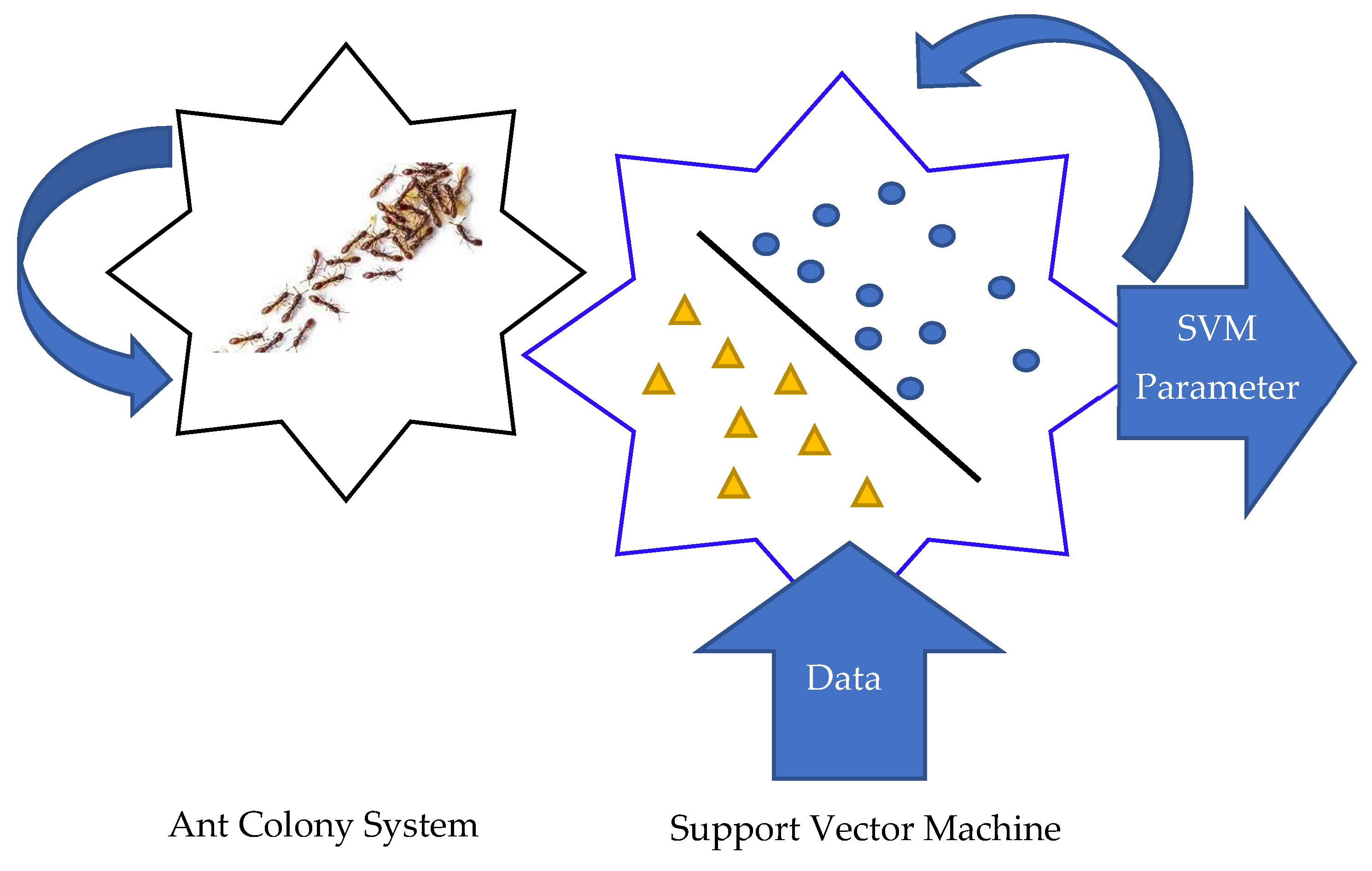
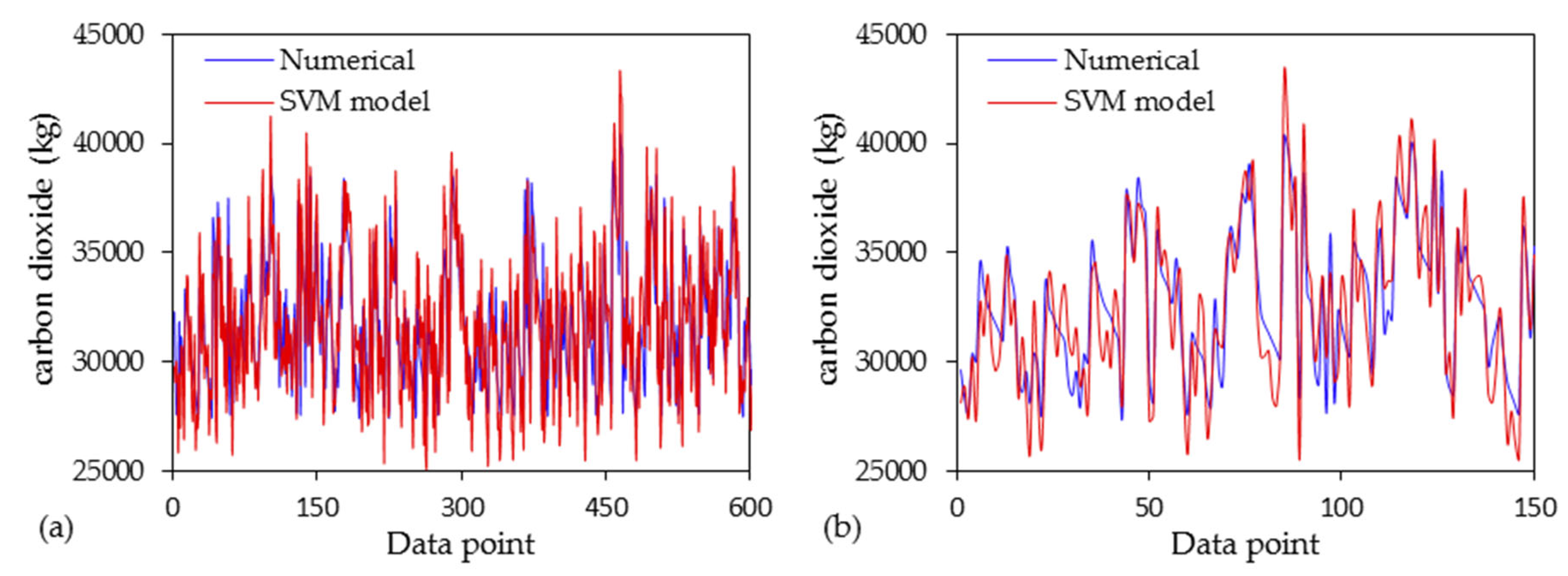
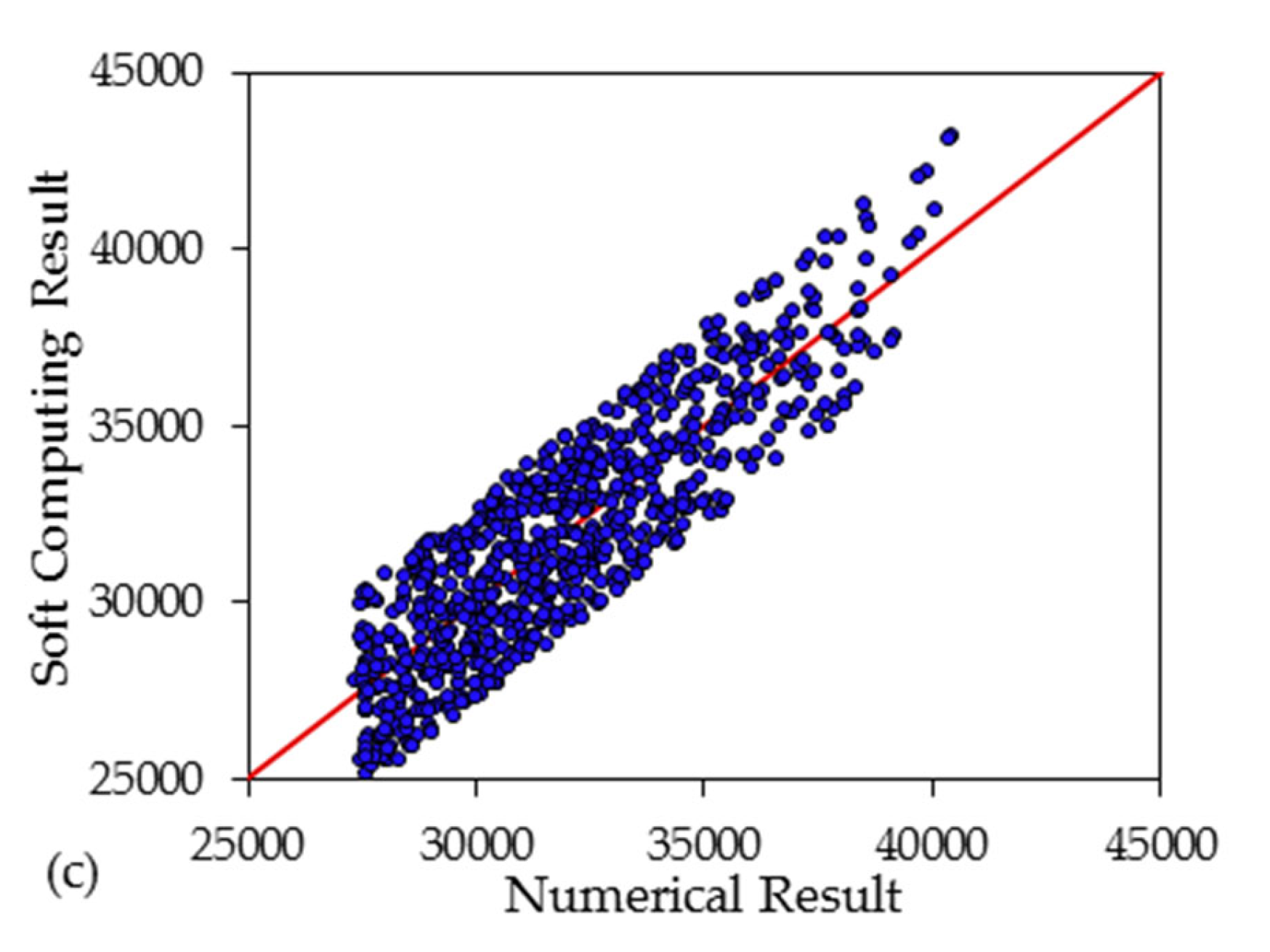
2.3. Support Vector Machine (SVM)

Vapnik and Chapelle [24] developed the support vector machine (SVM), a two-tier classification approach incorporating observer learning. In this strategy, structural risk minimization (SRM) principles are employed to reduce the model error. Other methods (such as the method of artificial neural networks) employ experimental risk minimization (ERM) concepts.

Classification and regression problems requiring three or more categories are ideal candidates for SVR’s use. Like many other machine learning techniques, this one has a two-step model-building process that consists of training and testing [25]. At the completion of the training process, the generalizability of the trained model is evaluated using test data. In practice, the support vector machine estimates the regression function using a series of linear functions. In this function, it is permissible to differ from the expected value (loss function). The ideal solution is then identified by applying structural risk reduction concepts to the loss-function-measured risk [26,27].

Solving the regression problem on a set of data in the form of $\left\{\left(x_1,y_1\right), \dots \left(x_1,y_1\right)ϵR^m yϵR\right\}$ is a linear function in the form of Equation (1) that can estimate the output values based on the inputs.

$$f\left(x\right)=\langle w.x\rangle +b$$

(1)

In the data set and Equation (1) x is the input vector (x ∈ R^m y), y is the output value (y ∈ R^m), w is the weight vector (w ∈ R^m), and b is the bias (b ∈ R^m)

The following optimization problem may be solved to acquire the control parameters of the optimal response function in SVM; that is, the weight and bias function. The loss function is used to obtain these control parameters.

$$\begin{array}{c}\mathrm{Minimize} \Phi \left(\mathit{w},{\mathit{\zeta }}^{*},\mathit{\zeta }\right)=\frac{\parallel w{\parallel }^2}{2}+\mathit{C}\left(\sum {\zeta }_i^{*}+\sum \zeta \right)\hfill \\ {\mathit{y}}_{\mathit{i}}-\left(\left(\mathit{w}\cdot {\mathit{x}}_i\right)+\mathit{b}\right)\le \mathit{\epsilon }+{\mathit{\zeta }}_{\mathit{i}}\\ \mathrm{Subject} \mathrm{to} \left(\left(w_1{x}_i\right)+b\right)-y_i\le \epsilon +{\zeta }_i^{*}\begin{array}{ll}\hfill & {\zeta }_i,{\zeta }_i\ge 0\hfill \\ \hfill & \hfill i=1,2,\dots ,1\end{array}\hfill \end{array}$$

(2)

where $\parallel w{\parallel }^2$ is the weight vector norm and ${\zeta }_{\mathrm{i}}^{*} \mathrm{and} \zeta$ are slack.

In accordance with Lagrange’s theory, the optimization issue represented by Equation (3) may be recast as Lagrange’s function, which is as follows:

$$\begin{array}{c}\mathrm{L}\left({\alpha }^{*},\alpha \right)=-\epsilon {\displaystyle \sum _{\mathrm{i}=1}^1} \left({\alpha }_{\mathrm{i}}^{*}+{\alpha }_{\mathrm{i}}\right)+\hfill \\ {\displaystyle \sum _{\mathrm{i}=1}^1} {\mathrm{y}}_{\mathrm{i}}\left({\alpha }_{\mathrm{i}}^{*}-{\alpha }_{\mathrm{i}}\right)-\frac{1}{2}{\displaystyle \sum _{\mathrm{i}=1}^1} {\displaystyle \sum _{\mathrm{i}=1}^1} \left({\alpha }_{\mathrm{i}}^{*}-{\alpha }_{\mathrm{i}}\right)({\alpha }_{\mathrm{j}}^{*}-{\alpha }_{\mathrm{j}})\left({\mathrm{x}}_{\mathrm{i}}·{\mathrm{x}}_{\mathrm{j}}\right)\hfill \end{array}$$

(3)

By maximizing the above function under the following conditions, the coefficients α and α^* are obtained. These coefficients are called Lagrange coefficients.

$$\left\{\begin{array}{l}\sum {\alpha }_i^{*}=\sum {\alpha }_i\hfill \\ 0\le {\alpha }_i^{*}\le \mathrm{C}\hfill \\ 0\le {\alpha }_i\le \mathrm{C}\hfill \end{array}\right. \mathrm{for} i=1,2,\cdots ,1$$

(4)

In Equation (4), L represents the Lagrange function and C represents the penalty parameter or adjustment parameter. Notably, the aforementioned optimization issue may be handled using quadratic programming (QP) techniques. As a consequence, attaining the absolute maximum or minimum will be deterministic, and there is a chance of being caught in a local maximum or minimum. The final response will be arranged as follows:

$$\begin{array}{l}{w}_0={\displaystyle {\displaystyle \sum }_{supportvectors }}\left({\alpha }_i^{\ast }-{\alpha }_i\right)x_i\hfill \\ b_0=-(1/2)w_0\cdot \left[x_r+x_s\right]\hfill \\ f(x)={\displaystyle {\displaystyle \sum }_{supportvectors }}\left({\alpha }_i^{\ast }-{\alpha }_i\right)\left(x_i-x\right)+b_0\hfill \end{array}$$

(5)

In this equation, x_i is the input vector with which the model is trained, x is the input vector, x_r and x_s are two vectors, w₀ supports the optimal weight vector, and b₀ is the optimal bias value. Data whose corresponding Lagrange coefficients are non-zero are known as support vectors. From the point of view of geometry, these data have a bigger prediction error than $\pm \epsilon$, so the support vectors are not included in the range of $\pm \epsilon$ and it controls the number of support vectors. According to the relationship, it is observed that the data whose Lagrange coefficient are zero do not play a role in the final answer; in other words, they are support vectors that determine the final regression function with the optimal answer [24].

To build the support vector machine model, parameters C and $\epsilon$ are defined by the user. The parameter C is an adjustment parameter and can accept values from zero to infinity. When large values are assigned to this parameter, SVM does not allow errors to occur in the training data and the result will be a complex model, so the generalizability of the model decreases. On the other hand, when C tends to zero, the model can accept a large error; as a result, the complexity of the model will be less [24].

The parameter $\epsilon$ can also accept values from zero to infinity. The value of this parameter is very effective in the case of support vectors and as a result the efficiency of the model. Although the selection of very large values of $\epsilon$ causes a reduction in the number of support vectors, which is also desirable, reaching this goal by widening the interval is incorrect. On the other hand, very small values of this parameter require a large number of support vectors to be selected and the possibility of overfitting increases.

The problem of linear regression in SVM can be easily extended to nonlinear regression. For this purpose, kernel functions are used. Kernel functions map the data to a feature space in which it is possible to use linear regression. So far, various kernel functions have been introduced, among which they can be classified as polynomial kernels. The radial basis function has been pointed out [25,26].

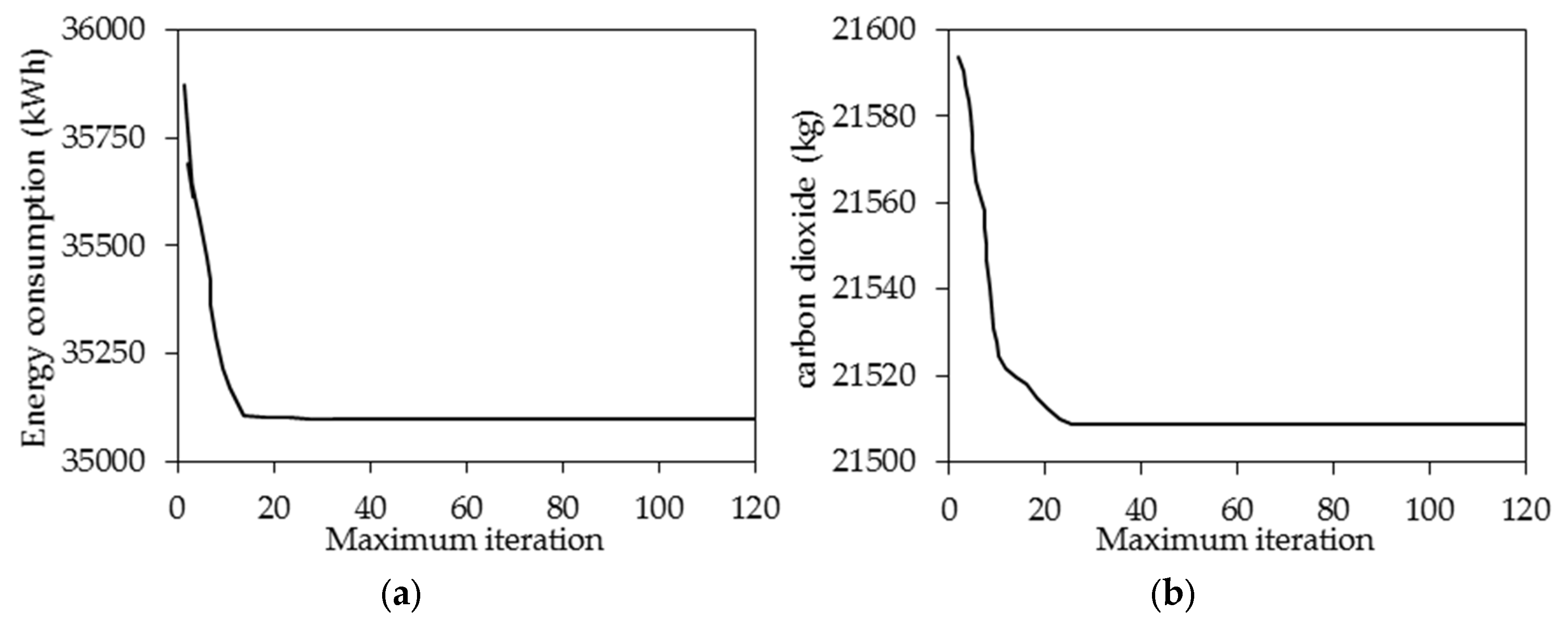
2.4. Ant Colony System (ACS)

This method, one of the innovative algorithms based on collective intelligence and population, is introduced as ant colony optimization [28]. The optimization of the ant colony, including a set of methods based on the behavior of the ant colony, is inspired by the search for food. To find food, ants do not follow the same route, which is the shortest possible route. Each ant emits a chemical substance called a pheromone along the way. All members of the colony sense the substance and direct their movement to the path that has more pheromone. In other words, the path with more pheromone will be more attractive to be chosen by an ant [29]. The ACS algorithm is one of the most efficient versions of the ants’ algorithm, and is currently used in various practical research problems. The purpose of the ACS algorithm is to determine the number of ants in a graph that corresponds to the optimal problem. Each ant can move in this graph in a possible way, and based on the amount of pheromone and innovative actions, it can respond. Then, the ants will determine the quantity of routes based on the quality of the generated answer, and in this way, the communication between the ants will be improved. The ants are a special kind of natural ants that have innovative obedience and memory to record their previous movements [30]. The heuristics are defined based on the objective function of the problem in such a way that it indicates the degree of improvement in the value of this function due to the movement of an ant from one node to another node. In addition, every movement that an artificial ant can make is stored in a memory, so that it can easily go back and restore the pheromone values. In addition, due to the complex structure of the problem, only a few applications of the ants’ algorithm have been used to solve the problem. This article presents the ACS method to solve the problem under study, which will be discussed in sufficient detail in the next sections. So far, different versions of the ACO algorithm have been presented [31]. Among these algorithms are the Ant Colony System Algorithm (AS), Max–Min Ant System (MMAS), and ACS. The main difference between the parts of the ACO algorithm is in the method of updating their pheromones [32]. The ACS algorithm is one of the most efficient ACO algorithms [33]. The main parameters using the algorithm are in Abbreviations.

Note that choosing q = 0 converts the ACS method to the AS method. Therefore, when and is less than equal, the ants use exploration to select the task as the next task in the schedule, while if it is greater, the ants use probability-based extraction to select the next task.

In this step, k numbers of ants are randomly assigned to one of the tasks of the problem. These tasks are the starting point for each ant to build its answer. We assign the value of ${\tau }_0$ to the power of the value of the first pheromone to all the arcs of the problem ($\forall \left(i,j\right){\tau }_{ij}={\tau }_0$) and the amount of bow pheromone is (i, j). Usually, the initial amount of pheromone is considered ${\tau }_0=\frac{1}{\left(n\times {\mathrm{HA}}_{-}\mathrm{Value}\right)}$ where HA_Value is the cost obtained by the heuristic algorithm.

In the solution-construction phase, each ant constructs a sequence in n steps. In each step, ant k, which is in the ith task, calculates j with the probability q₀ of its next task according to the Equation (6).

$$j=\arg \underset{l\in {\mathbb{N}}_i^k}{\mathit{max}}\{{\left[{\tau }_{il}\right]}^{\alpha }{\left[{\eta }_{il}\right]}^{\beta }\}$$

(6)

The ant considers the probability 1 − q₀ of its next task according to the Equation (7).

$$p_{ij}{}^k=\frac{{\left[{\tau }_{ij}\right]}^{\alpha }{\left[{\eta }_{ij}\right]}^{\beta }}{{\sum }_{l{\in }_i^k}{\left[{\tau }_{il}\right]}^{\alpha }{\left[{\eta }_{il}\right]}^{\beta }},\mathrm{if}j\in {\mathrm{N}}^k$$

(7)

where d_ij is the length of the bow (i, j), ${\eta }_{ij}=\frac{1}{d_{i{j}_{ }}}$ represents the influence of this innovative value, and β is the innovative value. N^k is the set of candidate actions of the ant for its next move.

After task j is selected for the next move of ant k, it is removed from N^k. In other words, until the end of the solution-creation process, ant k no longer has the right to choose the work. It should also be said that at the beginning of the solution-creation process, N^k = V 1 ≤ k ≤ K, where V is the set of all tasks of the problem.

Local updating of pheromones occurs during the solution-construction process. As soon as the bad ant passes an arc (i, j), the amount of pheromone on that arc is also updated according to Equation (8). This process is called local updating of pheromones.

$${\tau }_{ij}=\left(1-\rho \right){\tau }_{ij}+\rho {\tau }_{0 0<\rho <1}$$

(8)

When the process of building the answer for all ants is completed and the local search process is completed on all these answers, the global update process of pheromones is performed. In the global update of pheromones, only the root pheromone amount of the best answer obtained in each iteration, i.e., T^bs, is updated according to Equation (9).

$${\tau }_{ij}=\left(1-\rho \right){\tau }_{ij}+\rho \mathsf{\Delta }{\tau }_{ij}^{bs},\forall \left(i,j\right)\in T^{bs}$$

(9)

where $\rho$ is the evaporation rate, $\mathsf{\Delta }{\tau }_{ij}^{bs}=\frac{1}{C^{bs}}$, and $C^{bs}$ is the value of T^bs. Of course, these actions encourage other ants to repeat this tour.

The ACS algorithm is terminated if the number of repetitions of the algorithm reaches its maximum value, determined in the parameter setting. The flowchart of the study is presented in Figure 4.

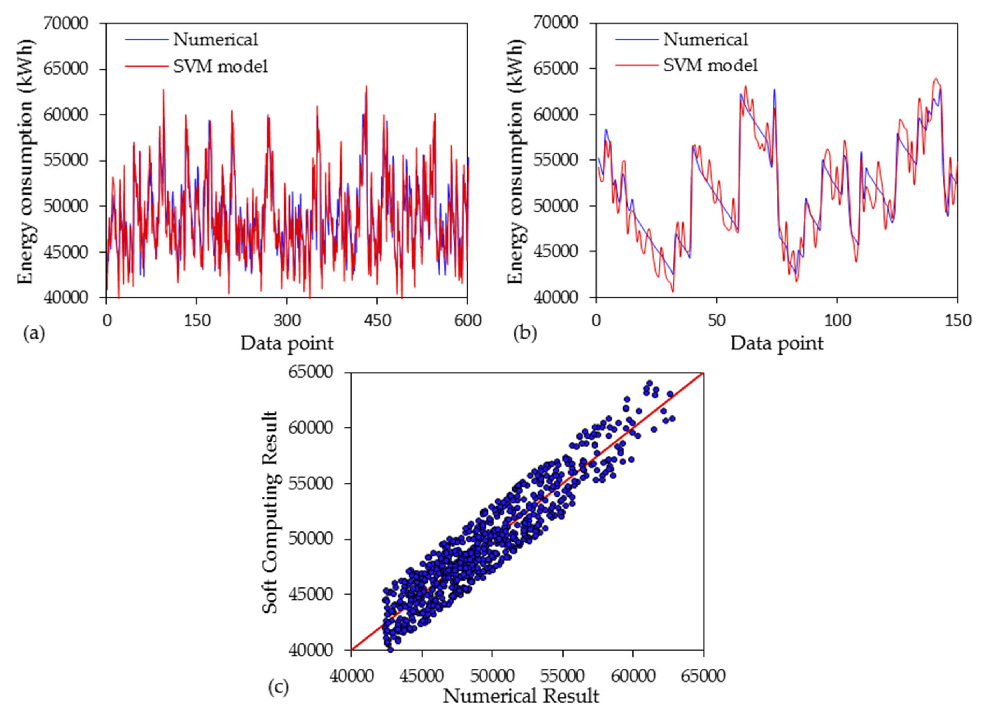
3. Results and Discussion

The number of test data is equivalent to 150, whereas the amount of training data is equal to 600. In this particular investigation, the characteristics of the wall, roof, and glass as well as the ideal percentage of window to wall in each of the four directions make up the inputs of the network. The weights and biases are the values that are assigned to the inputs and the amount of energy consumption and CO₂ makes up the output of the model. In other words, this research involved the training of two different networks: one network was trained to collect energy, while the second network was trained to obtain CO₂. Because training data and test data are both utilized in the process of training the network, the results that the network produces for these two distinct types of data have been analyzed.

The evaluation results of each of the models are evaluated for changes in ε values while other parameters are fixed, using the number of support vectors on the training set and the values of the correlation coefficient and the root mean square on the test data set. As $\epsilon$ increases, the number of support vectors decreases. In the process of reaching the optimal response, reducing the number of the support vector by increasing the value is effective up to a certain level, and reaching the least error in the prediction and the most correlation with the actual values is not necessary. By examining the extended models with the radial basis kernel function, it is observed that the model in which the width of the kernel function is equal to 1.5 and the $\epsilon$ is selected 0.007.

Figure 5a and Figure 6a illustrate, respectively, the amount of energy consumed and the amount of CO₂ produced by trains. The precision of the network’s training is demonstrated by the fact that the amount of energy that is computed by the network is very near to its actual value for each of the data points. Figure 5b and Figure 6b, meanwhile, illustrate the statistics on the use of energy and the production of CO₂, respectively, for the tests.

The scatter plot of the SVM model and the simulated results are shown in Figure 5c and Figure 6c, respectively. The comparison of the actual data with the data obtained from the network is shown in these figures, along with the best line that can be drawn through these points.

In general, in Figure 5 and Figure 6, the closeness of the modeled and estimated values can be seen well, and this indicates the correctness of the SVM model and the sameness of the results obtained from the network and what was actually performed. The statistical index and the performance of the model are presented in

Table 3. Statistical performance of the SVR models.

Output	Stage	Statistical Index
		R	R2	RMSE
Energy consumption	Train	0.921	0.874	904 (kWh)
	Test	0.882	0.824	1012 (kWh)
CO2	Train	0.901	0.831	1129 (kg)
	Test	0.863	0.799	1076 (kg)

.

The results of Hui et al. [34] showed that depending on the geographical region, season, and direction of the building, it is possible to increase the temperature of the outer and inner surface to 27 and 1.0 degrees centigrade, respectively, by using different coatings. In the current research, insulation with a thickness of 5 cm was used in the wall and ceiling, which caused temperature and energy regulation. Therefore, the role of insulation and various coatings is important to reduce energy consumption.

4. Results of Optimization

As seen in the training of the network, the number of seven inputs includes the same input variables in the simulation. The number of outputs is two outputs, whose purpose is to minimize the amount of energy and CO₂. Therefore, ACS are executed once for energy consumption and once for CO₂, and the results are analyzed. The implementation of the algorithm shows that for both objective functions, the input values are almost the same.

Before implementing ACS to solve the problems, the algorithm parameters must be adjusted first. In this way, the most important parameters of the proposed algorithm, which have a significant effect on the convergence of the algorithm, are analyzed. For this purpose, different values are tested for each desired parameter, so that the best values for the investigated parameters are obtained in the selection process. In order to select quantitative variables, an experiment was designed according to the table, and for each number of tasks in each group, problems were randomly generated. Since the values of the parameters of the problem affect its current time, in this paper, different values are considered for a number of important parameters of the problem. This will show how the values of the parameters will affect the time to solve the problems. Parameter setting results for the method are shown in

Table 4. Parameter setting results for the method.

max_it	q0			β			α		ρ			k
120	0.6	0.79	0.98	1	3	5	1	2	0.1	0.5	0.9	2	5	8

.

The optimal values of the input parameters resulting from the implementation of ACS for the objective function of minimizing the amount of energy consumption and CO₂ production are given. The optimal energy consumption is equal to 3.512 × 10⁴ kWh and the amount of CO₂ production is equal to 2.151 × 10⁴ kg (Figure 7).

The optimal values of parameters include brick walls with insulation with a thickness of 40 mm, roof made of beams with insulation with a thickness of 40 mm, and triple-paned glass. According to the findings, the proportion of the north and east windows to the wall in one direction is 70 percent, and the proportion of the south window to the wall in that direction ranges between 35 and 50 percent. The amount of energy consumption and CO₂ dioxide that is produced is reduced to a negligible level when the ratio and percentage of the west window to the west wall is between 60 and 70 percent.

5. Conclusions

In this study, the current condition of an educational building in Jakarta, Indonesia was analyzed in terms of energy consumption and CO₂ emissions, and optimization was modeled using DesignBuilder, an SVM model, and an ACS algorithm. The application of ACS revealed that if the building includes a brick wall with 40 mm thick insulation, a beam roof with 40 mm thick insulation, three-pane glass, a proportion of north and east windows to the wall in the same direction of 60%, a proportion of the south window to the south wall between 10 and 14%, and a proportion of the west window to the west wall between 35 and 50%, the amount of energy and CO₂ is minimal.

Other effective methods for reducing energy consumption in buildings were investigated in this study, and the findings were generally associated with energy consumption optimization. This implies that by modifying the building’s parameters, its energy consumption can be reduced. In addition, applying a large number of these variables does not incur significant costs in the building, and on the contrary, they decreased the building’s current costs and the cost of energy. In this study, the parameters that lead to a reduction in energy consumption and CO₂ emissions are examined, including the optimal window-to-wall ratios in different building orientations. If the objective function of energy is chosen, the ACS results are in close agreement with the optimization results when the objective function is CO₂ concentration. In other words, the optimization of one objective function will result in the optimization of the other. Thus, we will not have to optimize two objectives for this specific problem. Consequently, the policy model for reducing greenhouse gases can also be presented. It is suggested that considering the climate conditions besides the building’s physical features should be evaluate in the model performance in future studies.

References

1. Molajou, A.; Afshar, A.; Khosravi, M.; Soleimanian, E.; Vahabzadeh, M.; Variani, H.A. A New Paradigm of Water, Food, and Energy Nexus. Environ. Sci. Pollut. Res. 2021, 28, 1–11. [Google Scholar] [CrossRef] [PubMed]
2. Molajou, A.; Pouladi, P.; Afshar, A. Incorporating Social System into Water-Food-Energy Nexus. Water Resour. Manag. 2021, 35, 4561–4580. [Google Scholar] [CrossRef]
3. Ahmadi, M.H.; Sayyaadi, H.; Dehghani, S.; Hosseinzade, H. Designing a Solar Powered Stirling Heat Engine Based on Multiple Criteria: Maximized Thermal Efficiency and Power. Energy Convers. Manag. 2013, 75, 282–291. [Google Scholar] [CrossRef]
4. Al Doury, R.R.J.; Salem, T.K.; Nazzal, I.T.; Kumar, R.; Sadeghzadeh, M. A Novel Developed Method to Study the Energy/Exergy Flows of Buildings Compared to the Traditional Method. J. Therm. Anal. Calorim. 2021, 145, 1151–1161. [Google Scholar] [CrossRef]
5. Ahmadi, M.H.; Jashnani, H.; Chau, K.W.; Kumar, R.; Rosen, M.A. Carbon Dioxide Emissions Prediction of Five Middle Eastern Countries Using Artificial Neural Networks. Energy Sources A Recovery Util. Environ. Eff. 2019, 41, 1–13. [Google Scholar] [CrossRef]
6. Yavari, F.; Salehi Neyshabouri, S.A.; Yazdi, J.; Molajou, A.; Brysiewicz, A. A Novel Framework for Urban Flood Damage Assessment. Water Resour. Manag. 2022, 36, 1991–2011. [Google Scholar] [CrossRef]
7. Azizi, H.; Nejatian, N. Evaluation of the Climate Change Impact on the Intensity and Return Period for Drought Indices of SPI and SPEI (Study Area: Varamin Plain). Water Supply 2022, 22, 4373–4386. [Google Scholar] [CrossRef]
8. Banan-Dallalian, M.; Shokatian-Beiragh, M.; Golshani, A.; Abdi, A. Use of a Bayesian Network for Storm-Induced Flood Risk Assessment and Effectiveness of Ecosystem-Based Risk Reduction Measures in Coastal Areas (Port of Sur, Sultanate of Oman). Ocean Eng. 2023, 270, 113662. [Google Scholar] [CrossRef]
9. Alayi, R.; Mohkam, M.; Seyednouri, S.R.; Ahmadi, M.H.; Sharifpur, M. Energy/Economic Analysis and Optimization of on-Grid Photovoltaic System Using CPSO Algorithm. Sustainability 2021, 13, 12420. [Google Scholar] [CrossRef]
10. Sedlmeir, J.; Buhl, H.U.; Fridgen, G.; Keller, R. The Energy Consumption of Blockchain Technology: Beyond Myth. Bus. Inf. Syst. Eng. 2020, 62, 599–608. [Google Scholar] [CrossRef]
11. Aruga, K.; Islam, M.M.; Jannat, A. Effects of COVID-19 on Indian Energy Consumption. Sustainability 2020, 12, 5616. [Google Scholar] [CrossRef]
12. Ren, S.; Hao, Y.; Xu, L.; Wu, H.; Ba, N. Digitalization and Energy: How Does Internet Development Affect China’s Energy Consumption? Energy Econ. 2021, 98, 105220. [Google Scholar] [CrossRef]
13. Osobajo, O.A.; Otitoju, A.; Otitoju, M.A.; Oke, A. The Impact of Energy Consumption and Economic Growth on Carbon Dioxide Emissions. Sustainability 2020, 12, 7965. [Google Scholar] [CrossRef]
14. Olu-Ajayi, R.; Alaka, H.; Sulaimon, I.; Sunmola, F.; Ajayi, S. Building Energy Consumption Prediction for Residential Buildings Using Deep Learning and Other Machine Learning Techniques. J. Build. Eng. 2022, 45, 103406. [Google Scholar] [CrossRef]
15. Li, X.; Zhou, Y.; Yu, S.; Jia, G.; Li, H.; Li, W. Urban Heat Island Impacts on Building Energy Consumption: A Review of Approaches and Findings. Energy 2019, 174, 407–419. [Google Scholar] [CrossRef]
16. Robinson, C.; Dilkina, B.; Hubbs, J.; Zhang, W.; Guhathakurta, S.; Brown, M.A.; Pendyala, R.M. Machine Learning Approaches for Estimating Commercial Building Energy Consumption. Appl. Energy 2017, 208, 889–904. [Google Scholar] [CrossRef]
17. Bourdeau, M.; Zhai, X.Q.; Nefzaoui, E.; Guo, X.; Chatellier, P. Modeling and Forecasting Building Energy Consumption: A Review of Data-Driven Techniques. Sustain. Cities Soc. 2019, 48, 101533. [Google Scholar] [CrossRef]
18. Yuan, S.; Hu, Z.Z.; Lin, J.R.; Zhang, Y.Y. A Framework for the Automatic Integration and Diagnosis of Building Energy Consumption Data. Sensors 2021, 21, 1395. [Google Scholar] [CrossRef]
19. Sharghi, E.; Nourani, V.; Molajou, A.; Najafi, H. Conjunction of Emotional ANN (EANN) and Wavelet Transform for Rainfall-Runoff Modeling. J. Hydroinform. 2019, 21, 136–152. [Google Scholar] [CrossRef]
20. Ahmadi, M.H.; Kumar, R.; Assad, M.E.H.; Ngo, P.T.T. Applications of Machine Learning Methods in Modeling Various Types of Heat Pipes: A Review. J. Therm. Anal. Calorim. 2021, 146, 2333–2341. [Google Scholar] [CrossRef]
21. Mojtahedi, A.; Dadashzadeh, M.; Azizkhani, M.; Mohammadian, A.; Almasi, R. Assessing Climate and Human Activity Effects on Lake Characteristics Using Spatio-Temporal Satellite Data and an Emotional Neural Network. Environ. Earth Sci. 2022, 81, 61. [Google Scholar] [CrossRef]
22. Liu, Y.; Chen, H.; Zhang, L.; Wu, X.; Wang, X.J. Energy Consumption Prediction and Diagnosis of Public Buildings Based on Support Vector Machine Learning: A Case Study in China. J. Clean. Prod. 2020, 272, 122542. [Google Scholar] [CrossRef]
23. Walker, S.; Khan, W.; Katic, K.; Maassen, W.; Zeiler, W. Accuracy of Different Machine Learning Algorithms and Added-Value of Predicting Aggregated-Level Energy Performance of Commercial Buildings. Energy Build. 2020, 209, 109705. [Google Scholar] [CrossRef]
24. Vapnik, V.; Chapelle, O. Bounds on Error Expectation for Support Vector Machines. Neural Comput. 2000, 12, 2013–2036. [Google Scholar] [CrossRef] [PubMed]
25. Shao, Y.H.; Chen, W.J.; Liu, L.M.; Deng, N.Y. Laplacian Unit-Hyperplane Learning from Positive and Unlabeled Examples. Inf. Sci. 2015, 314, 152–168. [Google Scholar] [CrossRef]
26. Wang, Y.; Wang, Y.; Song, Y.; Xie, X.; Huang, L.; Pang, W.; Coghill, G.M. An Efficient V-Minimum Absolute Deviation Distribution Regression Machine. IEEE Access 2020, 8, 85533–85551. [Google Scholar] [CrossRef]
27. Li, Y.; Wang, Y.; Bi, C.; Jiang, X. Revisiting Transductive Support Vector Machines with Margin Distribution Embedding. Knowl.-Based Syst. 2018, 152, 200–214. [Google Scholar] [CrossRef]
28. Ouaddi, K.; Benadada, Y.; Mhada, F.Z. Ant Colony System for Dynamic Vehicle Routing Problem with Overtime. Int. J. Adv. Comput. Sci. Appl. 2018, 9, 306–315. [Google Scholar] [CrossRef]
29. Chu, S.C.; Roddick, J.F.; Pan, J.S. Ant Colony System with Communication Strategies. Inf. Sci. 2004, 167, 63–76. [Google Scholar] [CrossRef]
30. Elsayed, E.K.; Omar, A.H.; Elsayed, K.E. Smart Solution for STSP Semantic Traveling Salesman Problem via Hybrid Ant Colony System with Genetic Algorithm. Int. J. Intell. Eng. Syst. 2020, 13, 476–489. [Google Scholar] [CrossRef]
31. Gajpal, Y.; Abad, P. An Ant Colony System (ACS) for Vehicle Routing Problem with Simultaneous Delivery and Pickup. Comput. Oper. Res. 2009, 36, 3215–3223. [Google Scholar] [CrossRef]
32. Liu, X.F.; Zhan, Z.H.; Deng, J.D.; Li, Y.; Gu, T.; Zhang, J. An Energy Efficient Ant Colony System for Virtual Machine Placement in Cloud Computing. IEEE Trans. Evol. Comput. 2018, 22, 113–128. [Google Scholar] [CrossRef]
33. Opoku, E.A.; Ahmed, S.E.; Song, Y.; Nathoo, F.S. Ant Colony System Optimization for Spatiotemporal Modelling of Combined EEG and MEG Data. Entropy 2021, 23, 329. [Google Scholar] [CrossRef]
34. Shen, H.; Tan, H.; Tzempelikos, A. The Effect of Reflective Coatings on Building Surface Temperatures, Indoor Environment and Energy Consumption—An Experimental Study. Energy Build. 2011, 43, 573–580. [Google Scholar] [CrossRef]
Figure 1. Jakarta, Indonesia’s location in the South Pacific Ocean (https://cdn.worlddata.info/pics/countrymaps/IDN.png (accessed on 10 May 2017)).
Sustainability 15 03118 g001
Figure 2. The modeled building characteristics and scheme.
Sustainability 15 03118 g002
Figure 3. A comparison of numerical outcomes and real data.
Sustainability 15 03118 g003
Figure 4. An overview of the ACS and SVM model architecture.
Sustainability 15 03118 g004
Figure 5. Comparison of the SVM-model-predicted energy consumption for (a) training data and (b) test data, and (c) scatter plot of the SVM and numerical results.
Sustainability 15 03118 g005
Figure 6. Comparison of the SVM-model-predicted CO2 production for (a) training data and (b) test data, and (c) scatter plot of the SVM and numerical results.
Sustainability 15 03118 g006aSustainability 15 03118 g006b
Figure 7. The results of (a) energy consumption and (b) CO2 production variation in terms of 120 maximum iterations.
Sustainability 15 03118 g007