
Numerical Design and Optimisation of Self-Compacting High Early-Strength Cement-Based Mortars

1
CONSTRUCT-LABEST, Faculty of Engineering, University of Porto, 4200-465 Porto, Portugal
2
Faculty of Engineering, University of Porto, 4200-465 Porto, Portugal
3
CMUP, Faculty of Sciences, University of Porto, 4200-465 Porto, Portugal
4
Faculty of Exact Sciences and Engineering, Campus da Penteada, University of Madeira, 9020-105 Funchal, Portugal
*
Author to whom correspondence should be addressed.
Appl. Sci. 2023, 13(7), 4142; https://doi.org/10.3390/app13074142
Submission received: 17 February 2023
/
Revised: 20 March 2023
/
Accepted: 21 March 2023
/
Published: 24 March 2023
(This article belongs to the Section Civil Engineering)
Abstract
:The use of SCC in Europe began in the 1990s and was mainly promoted by the precast industry. Precast companies generally prefer high early-strength concrete mixtures to accelerate their production rate, reducing the demoulding time. From a materials science point of view, self-compacting and high early-strength concrete mixes may be challenging because they present contradicting mixture design requirements. For example, a low water/binder ratio (w/b) is key to achieving high early strength. However, it may impact the self-compacting ability, which is very sensitive to Vw/Vp. As such, the mixture design can be complex. The design of the experimental approach is a powerful tool for designing, predicting, and optimising advanced cement-based materials when several constituent materials are employed and multi-performance requirements are targeted. The current work aimed at fitting models to mathematically describe the flow ability, viscosity, and mechanical strength properties of high-performance self-compacting cement-based mortars based on a central composite design. The statistical fitted models revealed that Vs/Vm exhibited the strongest (negative) effect on the slump-flow diameter and T-funnel time. Vw/Vp showed the most significant effect on mechanical strength. Models were then used for mortar optimisation. The proposed optimal mixture represents the best compromise between self-compacting ability—a flow diameter of 250 mm and funnel time equal to 10 s—and compressive strength higher than 50 MPa at 24 h without any special curing treatment.
1. Introduction
The building and construction industries have a heavy environmental impact. They account for 40% of natural resources, consume 70% of electrical power and 12% of potable water, and produce 45–65% of landfilled waste and 48% of GHG emissions [1]. In Europe, construction is the most significant economic sector, employing 18 million people directly and creating close to 10% of the European Union Gross Domestic Product. Thus, construction is an essential pillar in the context of the 2030 Agenda since it impacts the economic, environmental, and social spheres.
Concrete is a massively used construction material and the second most-consumed material worldwide, just after water [2]. This is mainly because the basic constituents, cement, aggregates, and water, are widely available worldwide; thus, concrete can be produced locally and consequently, it is inexpensive. Moreover, it hardens quickly and in all habitable environments, including underwater.
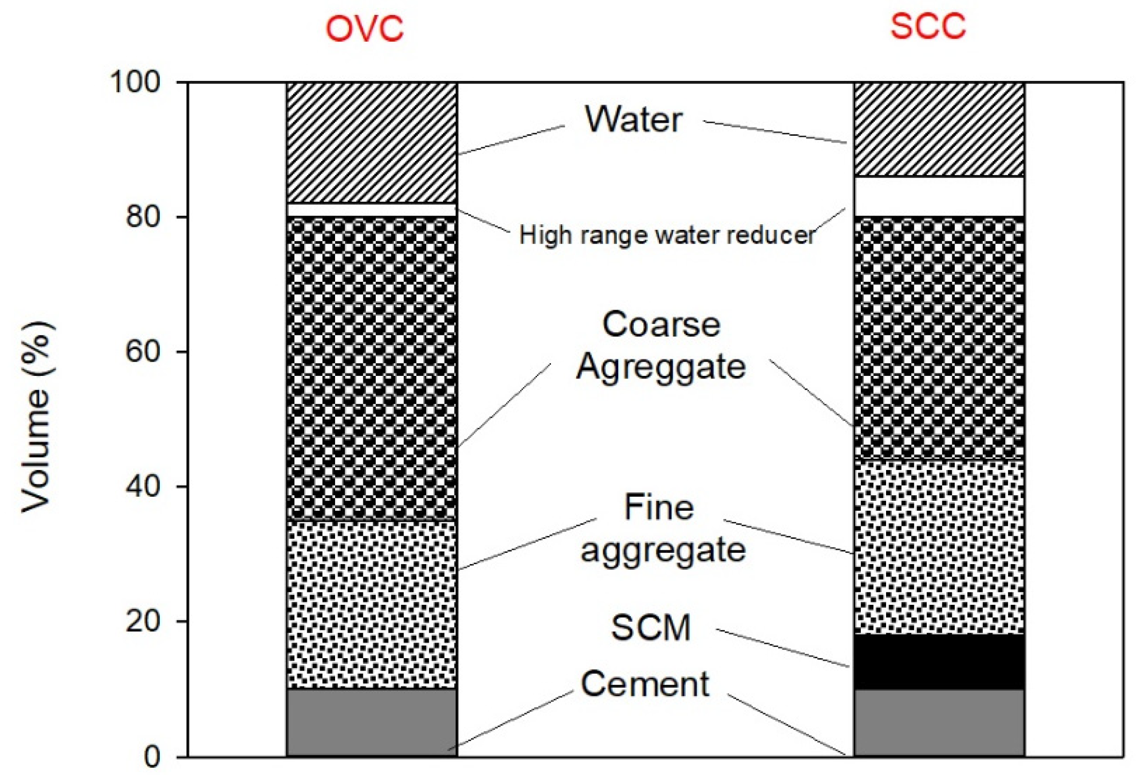
Over recent decades, efforts have been made to improve the behaviour of concrete materials. It took more than 150 years from the patenting of Portland cement (in 1824) until the discovery and development of self-compactable concrete (SCC) in the 1980s in Japan [3,4]. The development of superplasticisers allowed the efficient dispersal of cementitious particles and the emergence of SCC. According to the European standard EN 206-1 (specification, performance, production, and conformity of concrete), the constituent raw materials of SCC are similar to ordinary vibrated concrete (OVC). The main differences between OVC and SCC are due to the constituents’ proportions. Figure 1 presents the indicative volumetric proportions of SCC and OVC [5]. As can be seen, the main difference between SCC and OVC is a higher dosage of fine materials, i.e., cement and supplementary cementitious materials (SCM), and a smaller amount of coarse aggregate and smaller particle size distribution [6].
As such, the design of more advanced cement-based materials such as SCC can be complex since several requirements must co-exist, such as (i) engineering properties, (ii) architecture, (iii) cost, and (iv) eco-efficiency, among others. Even though the selection of the material should try to improve robustness, making the mixture more tolerant to raw material variability, for economic reasons, depends significantly on local availability; hence, there is no fixed rule for the amount/type of aggregates, cement, additions, and admixtures [6]. Therefore, a decisive factor for designing advanced cementitious materials, such as self-compacting concrete (SCC), is a clear understanding of each constituent raw material’s effect and interactions on the final product properties [7]. Additionally, the design and optimisation of such mixtures require intensive laboratory testing, particularly if new and unconventional supplementary cementitious materials or aggregates are incorporated [8], such as agricultural or industrial by-products [9]. Thus, a more scientific and multi-scale approach to mix-design is needed in which key mixture design variables can explain the composite properties [10].
The Design of Experiments (DoE) is a systematic approach to understanding how process and product parameters affect response variables, such as processability, physical properties, or product performance. DoE uses statistical methodology to analyse data and predict product property performance under all possible conditions within limits selected for the experimental design [10]. From a literature survey, the DoE approach [11] has shown promise for aiding the understanding of the effect of mixture parameters on key fresh and hardened SCC properties. It can also facilitate the test protocol required to optimise SCC [12] or quantify SCC mixtures’ robustness [6] to develop a more eco-friendly SCC that incorporates different types of SCM and meets multiple performance requirements [3,13,14,15,16,17,18,19,20,21].
Research Significance and Objectives
Previous research shows that statistical models and numerical optimisation techniques allow for finding the best combination of self-compacting high-strength concrete (SCHPC) constituents which (i) reduce the risk of cracking during the first days, ensuring a more impermeable concrete in the final structure [3]; (ii) study the influence of mixture parameters and their coupled effects on deformability, viscosity, compressive strength, resistivity and resistance to carbonation [15]; (iii) optimise chloride permeability and the strength of concrete containing metakaolin [22]; (iv) optimise the durability and service life of self-consolidating concrete containing metakaolin [19]; (v) optimise the mixture proportions and analyse the fresh and hardened properties [20]; and (vi) minimise the cost of the most unsustainable concrete components [21], including cost and sustainability indicators, in a reduced time [3,14,21,23]. These models and counterplot charts are beneficial for predicting and selecting the optimum mixture proportions for a given application simply and accurately.
From a materials science point of view, self-compacting and high early-strength concrete mixes may be challenging because they contradict mixture design requirements and fresh-state properties. For example, a low water/binder ratio (w/b) is key to achieving high early strength [24]. However, it may also impact self-compacting ability, which is very sensitive to Vw/Vp.
Maia [25] carried out a full central composite design on self-compacting high early-strength cement-based mortars (SCHSCM) based on key mixture design parameters and described the target engineering properties, namely, self-compacting ability and high early-age strength. The key five SCHSM mixture parameters chosen were [25]: (i) Vw/Vc—water to cement volume ratio; (ii) Sp/p—superplasticiser to powder mass ratio; (iii) Vw/Vp—water to powder volume ratio; (iv) Vs/Vm—sand to mortar volume ratio; and (v) Vfs/Vs—fine sand to total sand volume ratio to produce a total of 50 SCHSM mixtures. The current work aims at statistical analysis, model fitting, validation, and optimisation of the data experiments carried out by Maia [25]. As such, combining the statistical design methods and regression analysis allowed for creating a model to mathematically describe the flow ability, viscosity, and flexural and compressive strength of SCHSCM. The models obtained were validated and used to optimise self-compacting mixtures with additional high early-age strength. The goal was to develop SCHSM with a minimum slump flow of 250 mm, flow time of 10 s, and compressive strength of at least 50 MPa at 24 h without any special curing treatment.
The current work starts with a brief explanation of the data obtained by Maia [25] in Section 2. The model’s fitting and adequacy are detailed in Section 3, and Section 4 presents the optimisation of SCHSCM, considering the performance requirements established by the authors. Finally, Section 5 presents the main conclusions.
2. Central Composite Design
In general, the DoE involves the following key steps: (i) a choice of factors (mixture parameters), levels, and ranges; (ii) a selection of response variable(s); (iii) a choice of experimental design; (iv) performing the experiments; (v) a statistical analysis of the data (fitting a model); and (vi) other computations with response models. The current work focused on steps (iv) and (v). A brief explanation of the design adopted is presented in Section 2.1, and the output properties are discussed in Section 2.2.
2.1. Experiment Definition and Planning
The present work sought to analyse 50 mortar mixes published by Maia [25] using DoE, the statistical methodology to analyse data and predict properties. It was necessary to integrate simple and conventional statistical methods into the experimental design methodology to draw statistically sound conclusions from the experiment. Subsequently, the commercial software Design-Expert was employed in the current study to develop a polynomial regression model.
Maia’s data set [25] corresponds to a full central 25 composite design augmented by 10 axial runs plus 8 central runs. It allows for the development of a polynomial regression model for each response variable as a function of the five design variables considered in that study (key factors): (i) Vw/Vc—water to cement volume ratio; (ii) Sp/p—superplasticiser to powder mass ratio; (iii) Vw/Vp—water to powder volume ratio; (iv) Vs/Vm—sand to mortar volume ratio; and (v) Vfs/Vs—fine sand to total sand volume ratio. In addition to the 50 mixes previously described, 14 extra mixes were produced to allow for comparing and validating the results of the response models. The effect of each key factor was evaluated at five levels −α, −1, 0, +1, and +α, as shown in Table 1. To make the design rotatable, the value of α was equal to nF1/4, where nF is the number of points in the factorial part of the design. In the current study, this corresponds to α equal to 2.378.
The self-compacting mortars were produced with the following commercial materials available (in Portugal): (i) cement CEM I 42.5 R with a specific gravity of 3100 g/m3, (ii) limestone filler with a specific gravity of 2680 kg/m3, (iii) siliceous natural sands with a maximum particle size of 4 mm, specific gravity of 2620 kg/m3, and water absorption of 0.40%, (iv) fine siliceous sand with a maximum particle size of 2 mm, specific gravity of 2630 kg/m3, and water absorption of 0.20%, and (v) a polycarboxylate based superplasticiser with a specific gravity of 1080 kg/m3 and solid content of 40% [25].
Four dependent variables (i.e., response variables) were considered: (i) slump-flow diameter (D-flow); (ii) the time in the V-funnel (T-funnel); (iii) flexural strength at 24 h, determined by the three-point loading method (F,24 h); and (iv) uniaxial compressive strength at 24 h (Rc,24 h). Table 2 summarises the response variables and is followed by a brief explanation of the measurement procedures to access the dependent variables.
Immediately after production, the (mini) slump flow was assessed following the procedures of EFNARC [26]. The procedure consists, in brief, in filling the mini cone with the fresh composite and then taking the cone off and observing the flow capacity on a plane surface. When the fresh composite stops moving, two perpendicular diameters are measured, and the average value is considered the flow diameter (D-flow) in mm.
Additionally, the V-funnel test was performed to assess the viscosity and passing ability using the mini funnel according to EFNARC [26]. In brief, the fresh composite was poured into the funnel after production. Then, the trap door was opened, allowing the fresh composite to flow out under gravity, and the time for the discharge to complete (the flow time), i.e., when light is seen from above through the funnel, was recorded. These results showed a typical trend of an increase in slump-flow diameter with a reduction in flow time. After fresh tests, three specimens 40 × 40 × 160 {mm3} were moulded. The specimens were demoulded at 24 h, and the mechanical strength was assessed following EN 196-1 [27].
2.2. Results
The experimental results obtained by Maia concerning the D-flow, T-funnel, F,24 h, and Rc,24 h response variables used for model fitting (Section 3.2) are presented in Table 3, as well as 14 validation points (Vi). The D-flow results presented in Table 3 correspond to the average of the two results obtained by Maia [25]. The F,24 h corresponds to an average of three results for each CCD mortar point, and the Rc,24 h is the average of six results, based on Maia [25].
3. Response Models
3.1. Test Results Analysis
Table 4 presents the statistical summaries of all the experimental results obtained (Table 3) and the eight central point’s results only. The perception of the coefficient of variation on the central points (Ci) and all CCD points (all Ci, Fi, and CCi) predicts a good fit for the D-flow, T-funnel, and Rc,24 h. On the other hand, good fits are not expected for F,24 h given that the coefficient of variation evaluated on the central points (4.16%) is close to the coefficient of variation assessed on the 50 points of the CCD (6.93%).
3.2. Model Fitting
Design-Expert software was used to assist in analysing the results for each response variable by examining summary plots of the data; fitting a model using regression analysis and ANOVA; validating the model by examining the residuals for trends and outliers, leverage points, autocorrelation, and violation of statistical assumptions, in general; and interpreting the model graphically. A significance level of 5% was used throughout. A detailed description of this procedure is presented in Section 3.2 to Section 3.5. The central composite design adopted allows for estimating a full quadratic model, as shown in Equation (1) [28,29].
where Y represents the response variable; Xi corresponds to the design variables considered; β is used for model parameters (β0 is the independent term, βi represents the linear effect of Xi, βii represents the quadratic effect of Xi, and βij represents the linear-by-linear interaction between Xi and Xj); and ε is the fitting error. The model parameters (β0, βi, and βij) can be estimated through multilinear regression analysis. In the course of the analysis, some of the terms in Equation (1) may not be significant. The results of the fitting procedure for the four response variables are summarised in Table 5, Table 6, Table 7, Table 8, Table 9, Table 10, Table 11 and Table 12. The model generated with all observed values for D-flow and T-funnel resulted in a significant lack of fit. This fact led to the withdrawal of the axial runs for the D-flow results and also the inclusion of one term (Sp/p) × (Vfs/Vs) in the model because the term was considered the most significant among those excluded, due to its low p-value (0.0574). In the case of the T-funnel model, in addition to applying the inverse transformation as a recommended Box–Cox transformation to the response, one observation was removed (F15 = 26.33, see Table 3). The F,24 h and Rc,24 h fitting considered all runs and resulted in a non-significant lack of fit.
3.3. D-Flow Model
For the D-flow model, the authors decided not to include the axial points (CC1, CC2, CC3, CC4, CC5, CC6, CC7, CC8, CC9, and CC10) because the D-flow values contained a wide range of spread flow diameters, as presented in Section 2.2, from 168 to 398 mm. The attempt to fit a quadratic model led to a significant lack of fit when axial runs were included, due essentially to non-linearities that a quadratic model is not able to explain. Moreover, axial points are associated with high Cook’s distances and leverage points. Further research should be put into finding a non-linear model for D-flow response.
Table 5 presents the ANOVA for D-flow data considering the aforementioned conditions. The reduced quadratic model is significant. Examining the magnitude of the effects, it can be perceived that Vs/Vm (factor X4) and Vw/Vp (factor X3) are dominant compared to Sp/p (factor X2), Vw/Vc (factor X1), and Vfs/Vs (factor X5). The analysis of variance confirms the previous interpretation. In this case, Vw/Vc, Sp/p, Vw/Vp, and Vs/Vm are significant terms of the model, i.e., the main effects Vw/Vc, Sp/p, Vw/Vp, and Vs/Vm, and the second order effects, (Vw/Vc) × (Vw/Vp), (Vw/Vp) × (Vfs/Vs), and (Vw/Vc)2, are those that most significantly influence the response Y1: D-flow. The predicted R2 of 0.9683 is in reasonable agreement with the adjusted R2 of 0.9802 (i.e., the difference is less than 0.2). The coefficients of the estimated regression model for D-flow (in coded values) are presented in the second column of Table 6. Since the second-order effect (Vw/Vp) × (Vfs/Vs) is considered a significant factor, Vfs/Vs was added to the model. Furthermore, (Sp/p) × (Vfs/Vs) was forced to enter the model to avoid a significant lack of fit. Table 6 presents the model’s coefficients’ standard error and confidence intervals.

Table 5.
ANOVA for the D-flow response.
| Test for | Source | Sum of Squares | Degrees of Freedom | Mean of Square | F-Value | p-Value |
|---|---|---|---|---|---|---|
| Significance of Regression | Model | 59,008.65 | 11 | 5364.42 | 176.44 | <0.0001 |
| Residual | 851.29 | 28 | 30.4 | |||
| Total | 59,859.94 | 39 | ||||
| Lack of Fit | Lack of Fit | 774.79 | 21 | 36.89 | 3.38 | 0.0523 |
| Pure Error | 76.5 | 7 | 10.93 | |||
| Partial significance of each predictor variable | Vw/Vc | 2547.2 | 1 | 2547.2 | 83.78 | <0.0001 |
| Sp/p | 670.7 | 1 | 670.7 | 22.06 | <0.0001 | |
| Vw/Vp | 12,070.7 | 1 | 12,070.7 | 397.02 | <0.0001 | |
| Vs/Vm | 39,025.2 | 1 | 39,025.2 | 1283.59 | <0.0001 | |
| Vfs/Vs | 64.7 | 1 | 64.7 | 2.13 | 0.1558 | |
| (Vw/Vc) × (Sp/p) | 267.38 | 1 | 267.38 | 8.79 | 0.0061 | |
| (Vw/Vc) × (Vw/Vp) | 919.13 | 1 | 919.13 | 30.23 | <0.0001 | |
| (Vw/Vc) × (Vs/Vm) | 309.38 | 1 | 309.38 | 10.18 | 0.0035 | |
| (Sp/p) × (Vfs/Vs) | 114.38 | 1 | 114.38 | 3.76 | 0.0626 | |
| (Vw/Vp) × (Vfs/Vs) | 285.01 | 1 | 285.01 | 9.37 | 0.0048 | |
| (Vw/Vc)2 | 2734.89 | 1 | 2734.89 | 89.95 | <0.0001 |
The three most significant parameters are typed in bold, and the most significant term is also underlined.
Table 6.
D-flow model coefficients in terms of coded values.
| Factor | Coefficient Estimate | Standard Error | 95% CI Low | 95% CI High |
|---|---|---|---|---|
| Intercept | 343.75 | 1.95 | 339.76 | 347.74 |
| Vw/Vc | 8.92 | 0.9747 | 6.93 | 10.92 |
| Sp/p | 4.58 | 0.9747 | 2.58 | 6.57 |
| Vw/Vp | 19.42 | 0.9747 | 17.43 | 21.42 |
| Vs/Vm | −34.92 | 0.9747 | −36.92 | −32.93 |
| Vfs/Vs | −1.42 | 0.9747 | −3.42 | 0.5748 |
| Vw/Vc × Sp/p | −2.89 | 0.9747 | −4.89 | −0.894 |
| Vw/Vc × Vw/Vp | −5.36 | 0.9747 | −7.36 | −3.36 |
| Vw/Vc × Vs/Vm | 3.11 | 0.9747 | 1.11 | 5.11 |
| Sp/p × Vfs/Vs | 1.89 | 0.9747 | −0.106 | 3.89 |
| Vw/Vp × Vfs/Vs | 2.98 | 0.9747 | 0.9877 | 4.98 |
| (Vw/Vc)2 | −20.67 | 2.18 | −25.14 | −16.21 |
The three most significant parameters are typed in bold, and the most significant term is also underlined.
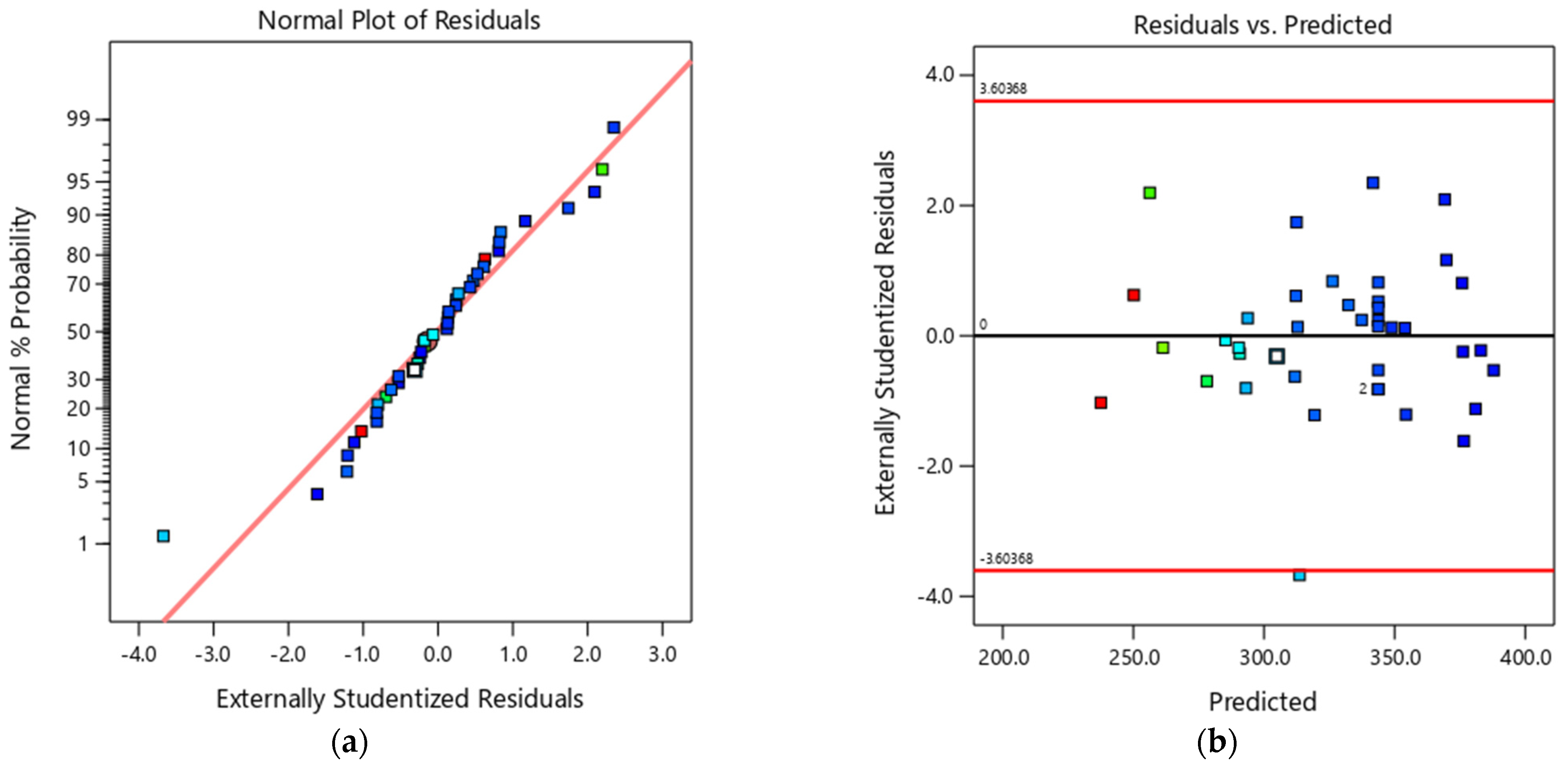
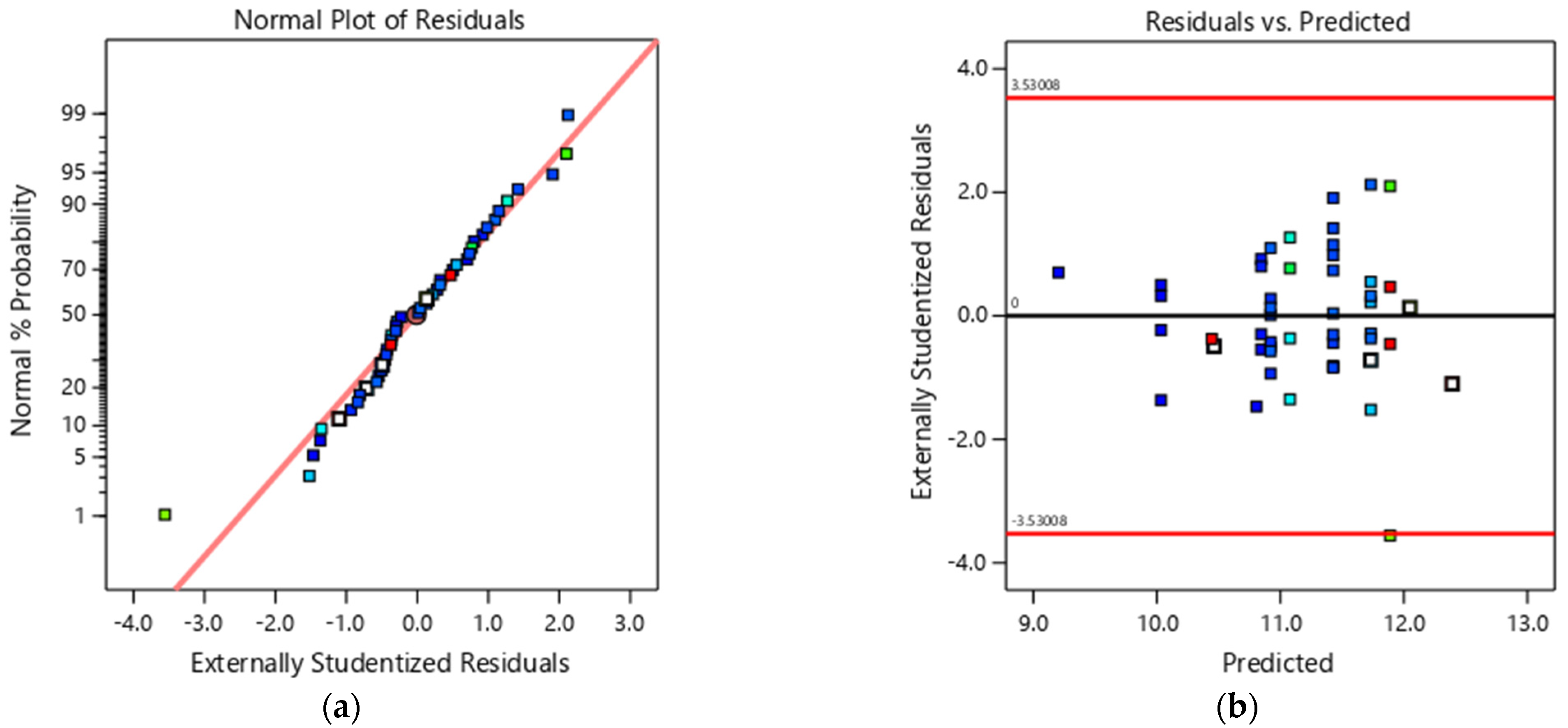
Figure 2a presents the normal probability plot of the model’s residuals. It is reasonable to consider that there are no relevant normality issues in the data. The plot of externally studentised residuals is presented in Figure 2b. One can notice an observation falls outside the −2 to +2 band, corresponding to the spreading diameter measurement of F5 with a value of 375 mm. It was decided to keep this observation since it did not constitute a leverage point, and the Cook’s distance was well below 50%.
3.4. T-Funnel Model
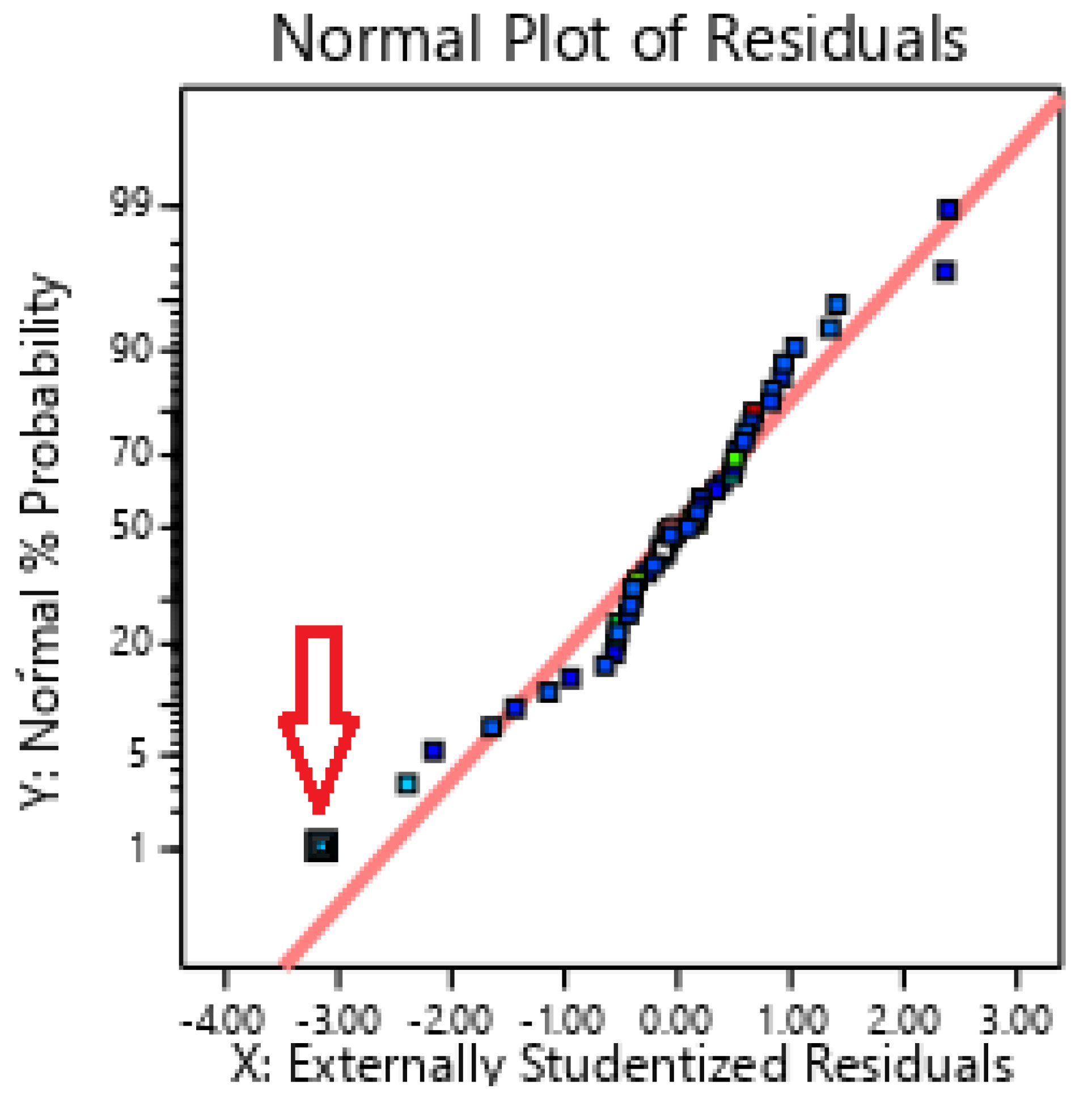
Regarding the T-funnel data, attempts to fit a quadratic model to all points lead to a severe lack of fit, potentially due to strong non-linearities. F15 exhibits an abnormal residual which compromises the fit; the following modelling steps exclude this point (see Figure 3).
The inverse transformation was applied to the T-funnel response, as found in previous works [3,14]. Examining the magnitude of the effects, it can be perceived that Vs/Vm (factor X4) and Vw/Vp (factor X3) are dominant compared to Sp/p (factor X2), Vw/Vc (factor X1), and Vfs/Vs (factor X5), as obtained in the D-flow response (see Table 7). All five factors are significant, as well as three of the interactions and the other three s-order terms. The predicted R2 of 0.9827 is in reasonable agreement with the adjusted R2 of 0.9897, i.e., the difference is negligible.
Table 7.
ANOVA results for the T-funnel response.
| Test for | Source | Sum of Squares | Degrees of Freedom | Mean of Square | F-Value | p-Value |
|---|---|---|---|---|---|---|
| Significance of Regression | Model | 0.0640 | 11 | 0.0058 | 394.23 | <0.0001 |
| Residual | 0.0005 | 34 | 0 | |||
| Total | 0.0645 | 45 | ||||
| Lack of Fit | Lack of Fit | 0.0005 | 27 | 0 | 3.14 | 0.0607 |
| Pure Error | 0 | 7 | 5.457 × 10⁻⁶ | |||
| Partial significance of each predictor variable | Vw/Vc | 0.0041 | 1 | 0.0039 | 305.22 | <0.0001 |
| Sp/p | 0.0010 | 1 | 0.0011 | 82.2 | <0.0001 | |
| Vw/Vp | 0.0251 | 1 | 0.0243 | 1895.62 | <0.0001 | |
| Vs/Vm | 0.0317 | 1 | 0.0271 | 2113.06 | <0.0001 | |
| Vfs/Vs | 0.0001 | 1 | 0.0001 | 6.9 | 0.0131 | |
| (Vw/Vc) × (Sp/p) | 0.0001 | 1 | 0.0001 | 11.61 | 0.0018 | |
| (Vw/Vc) × (Vs/Vm) | 0.0004 | 1 | 0.0003 | 23.66 | <0.0001 | |
| (Vw/Vp) × (Vs/Vm) | 0.0011 | 1 | 0.0009 | 73.86 | <0.0001 | |
| (Vw/Vc)2 | 0.0001 | 1 | 0.0001 | 6.79 | 0.0138 | |
| (Vw/Vp)2 | 0.0001 | 1 | 0.0001 | 4.84 | 0.0351 | |
| (Vfs/Vs)2 | 0.0001 | 1 | 0.0001 | 8.39 | 0.0067 |
The three most significant parameters are typed bold and the most significant term is also underlined.
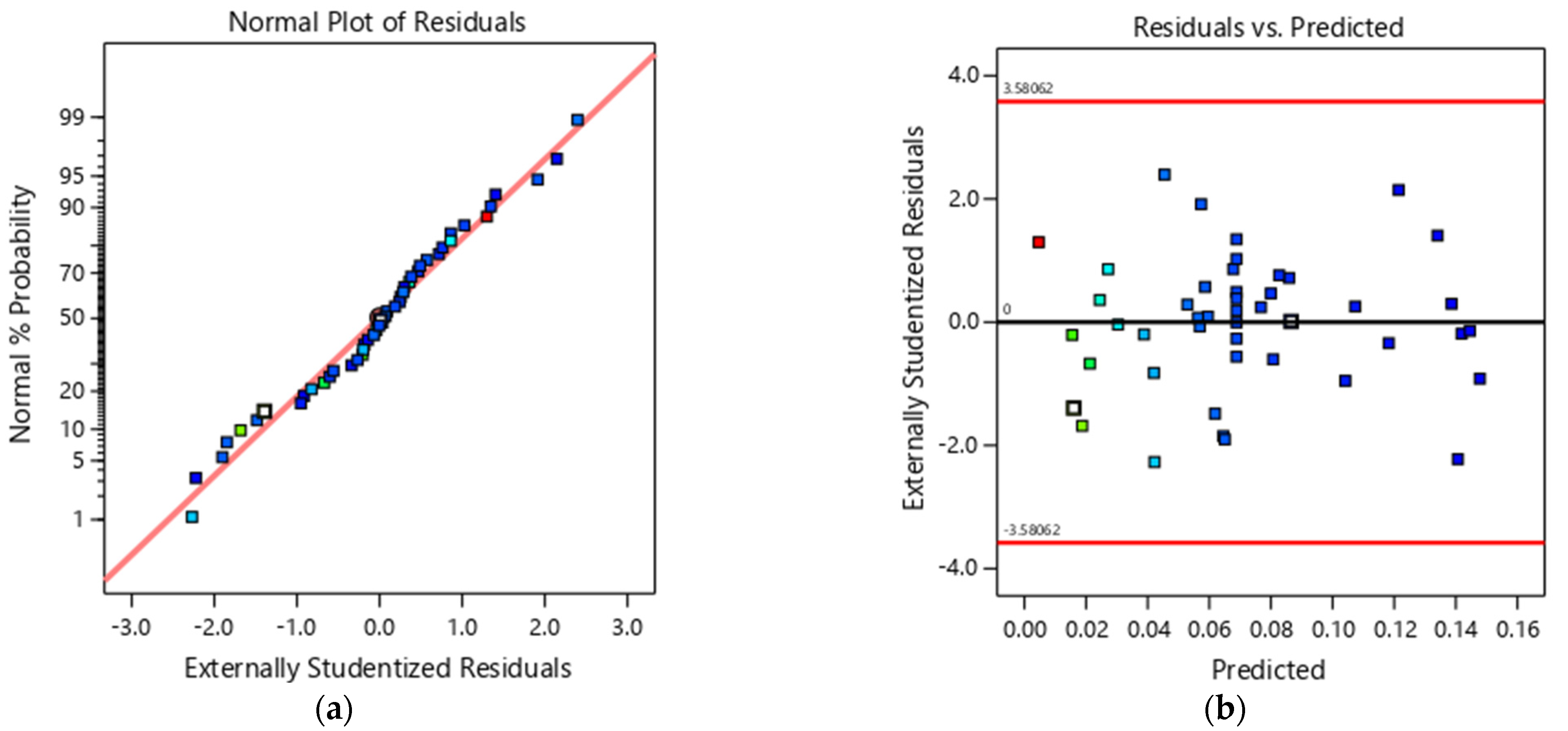
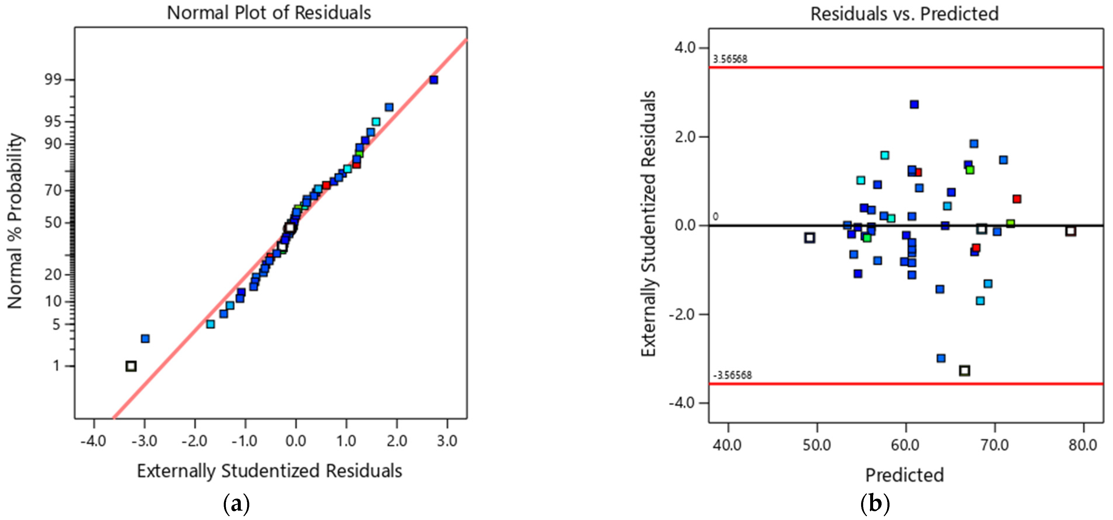
The estimated coefficients of the regression model for the T-funnel (in coded values) are presented in the second column of Table 8. Additionally, Table 8 presents standard errors and confidence intervals. To check the regression assumptions on the residuals, a normal probability plot was examined in Figure 4a and other plots such as the one in Figure 4b. No outliers were detected, although F15 has been considered a leverage point. In the author’s view, this point does not considerably compromise the fitted model’s quality.
Table 8.
T-funnel model coefficients (coded values).
| Factor | Coefficient Estimate | Standard Error | 95% CI Low | 95% CI High |
|---|---|---|---|---|
| Intercept | 0.0688 | 0.0011 | 0.0667 | 0.071 |
| Vw/Vc | 0.0115 | 0.0007 | 0.0101 | 0.0129 |
| Sp/p | 0.005 | 0.0006 | 0.0038 | 0.0062 |
| Vw/Vp | 0.0248 | 0.0006 | 0.0236 | 0.026 |
| Vs/Vm | −0.0302 | 0.0007 | −0.0315 | −0.0289 |
| Vfs/Vs | −0.0016 | 0.0006 | −0.0028 | −0.0004 |
| (Vw/Vc) × (Sp/p) | −0.002 | 0.0007 | −0.0035 | −0.0006 |
| (Vw/Vc) × (Vs/Vm) | −0.0037 | 0.0007 | −0.0051 | −0.0022 |
| (Vw/Vp) × (Vs/Vm) | −0.0061 | 0.0007 | −0.0076 | −0.0047 |
| (Vw/Vc)2 | −0.0017 | 0.0007 | −0.0031 | −0.0003 |
| (Vw/Vp)2 | 0.0011 | 0.0005 | 0.0001 | 0.0021 |
| (Vfs/Vs)2 | −0.0014 | 0.0005 | −0.0024 | −0.0003 |
The three most significant parameters are typed bold and the most significant term is also underlined.
3.5. Flexural Strength: F,24 h Model
No leverage points were found for the F,24 h model and the Cook’s distance was below 60%. Table 9 presents the ANOVA results for the F,24 h model. Examining the magnitude of the effects, it can be perceived that Vw/Vc (factor X1), Vw/Vp (factor X3), and Vs/Vm (factor X4) are dominant compared to Sp/p (factor X2) and Vfs/Vs (factor X5). The analysis of variance confirms the previous interpretation. The quadratic model is significant. In this case, Vw/Vc, Vw/Vp, and Vs/Vm are significant terms of the model, i.e., the main effects Vw/Vc, Vw/Vp, and Vs/Vm, and the second order effects (Vw/Vp) × (Vs/Vm) and (Vs/Vm)2 are those that most significantly influence the F,24 h response. The predicted R2 of 0.5671 is in reasonable agreement with the adjusted R2 of 0.6216 (i.e., the difference is less than 10%). Although R2 did not reach a value close to 1, the model was considered useful for navigating the design space.
Table 9.
ANOVA results for the F,24 h response.
| Test for | Source | Sum of Squares | Degrees of Freedom | Mean of Square | F-Value | p-Value |
|---|---|---|---|---|---|---|
| Significance of Regression | Model | 18.65 | 5 | 3.73 | 16.44 | <0.0008 |
| Residual | 9.53 | 42 | 0.2269 | |||
| Total | 28.18 | 47 | ||||
| Lack of Fit | Lack of Fit | 7.88 | 35 | 0.2252 | 0.9574 | 0.5812 |
| Pure Error | 1.65 | 7 | 0.2352 | |||
| Partial significance of each predictor variable | Vw/Vc | 7.11 | 1 | 7.11 | 31.36 | <0.0001 |
| Vw/Vp | 2.95 | 1 | 2.95 | 13.01 | 0.0008 | |
| Vs/Vm | 2.95 | 1 | 2.95 | 12.98 | 0.0008 | |
| (Vw/Vp) × (Vs/Vm) | 1.07 | 1 | 1.07 | 4.70 | 0.0358 | |
| (Vs/Vm)2 | 4.57 | 1 | 4.57 | 20.16 | <0.0001 |
The three most significant parameters are typed in bold, and the most significant term is also underlined.
The estimated values of the regression model coefficients in the coded values are presented in the second column of Table 10. Additionally, Table 10 presents standard errors and confidence intervals. Figure 5a presents the normal probability plot of the residuals of the observed values of flexural strength. The externally studentised residuals are presented in Figure 5b and show no strong evidence of violating the white noise assumptions of the remaining error in the regression model. It is reasonable to consider that there are no normality issues in the data.
Table 10.
F,24 h model coefficients in terms of coded values.
| Factor | Coefficient Estimate | Standard Error | 95% CI Low | 95% CI High |
|---|---|---|---|---|
| Intercept | 11.43 | 0.0893 | 11.25 | 11.61 |
| Vw/Vc | −0.4053 | 0.0724 | −0.5513 | −0.2592 |
| Vw/Vp | −0.261 | 0.0724 | −0.4071 | −0.115 |
| Vs/Vm | 0.2608 | 0.0724 | 0.1147 | 0.4068 |
| (Vw/Vp) × (Vs/Vm) | 0.1826 | 0.0842 | 0.0127 | 0.3525 |
| (Vs/Vm)2 | −0.2834 | 0.0631 | −0.4108 | −0.156 |
3.6. Compressive Strength: Rc,24 h Model
Table 11 presents the ANOVA results for Rc,24 h. Examining the magnitude of the effects, it can be perceived that Vw/Vc (factor X1), Vw/Vp (factor X3), and Vfs/Vs (factor X5) are dominant compared to Sp/p (factor X2). The reduced quadratic model is significant (p < 0.0001) and there is no lack of fit. The analysis of variance confirms the previous interpretation: Vw/Vc, Vw/Vp, and Vfs/Vs are significant terms of the model, i.e., the main effects Vw/Vc, Vw/Vp, and Vfs/Vs, the second order effects (Vs/Vm) × (Vfs/Vs), (Vw/Vc)2, and (Vw/Vp)2, are those that most significantly influence the response Rc,24 h. In addition, the predicted R2 of 0.9326 is reasonably close to the adjusted R2.
Table 11.
ANOVA results for the Rc,24 h response.
| Test for | Source | Sum of Squares | Degrees of Freedom | Mean of Square | F-Value | p-Value |
|---|---|---|---|---|---|---|
| Significance of Regression | Model | 1850.32 | 10 | 185.03 | 119.74 | <0.0001 |
| Residual | 60.26 | 39 | 1.35 | |||
| Cor Total | 1910.58 | 49 | ||||
| Lack of Fit | Lack of Fit | 51.87 | 32 | 1.62 | 1.35 | 0.3599 |
| Pure Error | 8.40 | 7 | 1.20 | |||
| Partial significance of each predictor variable | Vw/Vc | 1650.75 | 1 | 1650.75 | 879.84 | <0.0001 |
| Sp/p | 5.37 | 1 | 5.37 | 3.48 | 0.698 | |
| Vw/Vp | 61.35 | 1 | 61.35 | 39.70 | <0.0001 | |
| Vs/Vm | 3.05 | 1 | 3.05 | 1.98 | 0.1677 | |
| Vfs/Vs | 76.06 | 1 | 76.06 | 49.22 | <0.0001 | |
| (Vw/Vc) × (Vw/Vp) | 6.08 | 1 | 6.08 | 3.93 | 0.0545 | |
| (Vw/Vc) × (Vfs/Vs) | 7.09 | 1 | 7.09 | 4.59 | 0.0385 | |
| (Vs/Vm) × (Vfs/Vs) | 7.79 | 1 | 7.79 | 5.04 | 0.0305 | |
| (Vw/Vc)2 | 18.43 | 1 | 18.43 | 11.93 | 0.0013 | |
| (Vw/Vp)2 | 17.44 | 1 | 17.44 | 11.29 | 0.0018 |
The three most significant parameters are typed in bold, and the most significant term is also underlined.
The estimated values of the coefficients of the regression model that will be used to predict Rc,24 h in the coded values are presented in the second column of Table 12. Additionally, Table 12 shows the standard errors and confidence intervals. Figure 6a illustrates the normal probability plot of the residuals of the observed compressive strength values. It is reasonable to consider that there are no normality issues in the data. An example plot of the residuals against the predicted values is presented in Figure 6b. There is no evidence of assumption violation regarding the regression model fit.
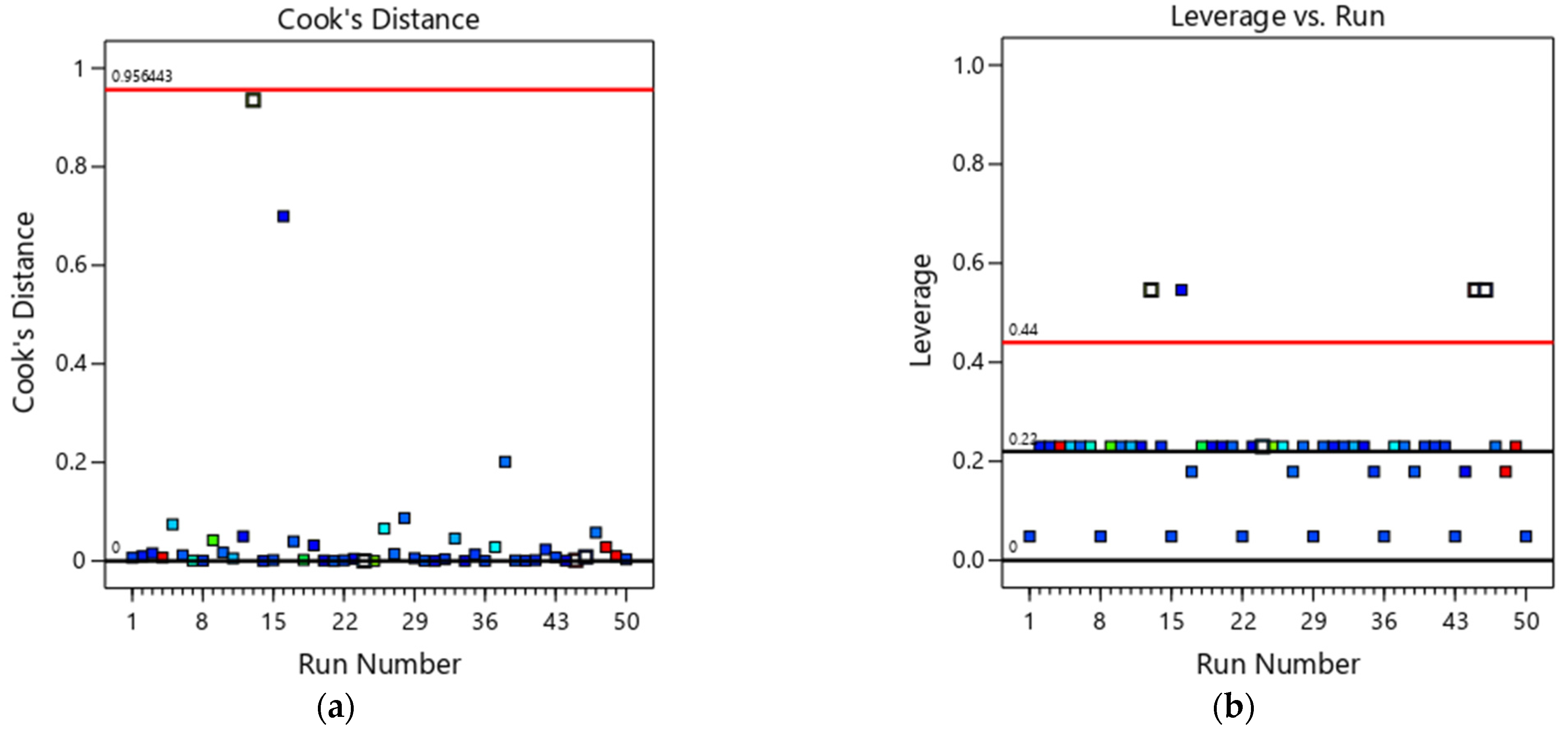
The subsequent diagnostics include the identification of possible outliers in the regression or observations that could be leverage points. Points with a Cook’s distance higher than 1.0 or high leverage were not found (see Figure 7).
Table 12.
Rc,24 h model coefficients in terms of coded values.
| Factor | Coefficient Estimate | Standard Error | 95% CI Low | 95% CI High |
|---|---|---|---|---|
| Intercept | 60.65 | 0.2733 | 60.09 | 61.2 |
| Vw/Vc | −6.17 | 0.1889 | −6.56 | −5.79 |
| Sp/p | −0.3522 | 0.1889 | −0.7342 | 0.0299 |
| Vw/Vp | −1.19 | 0.1889 | −1.57 | −0.8081 |
| Vs/Vm | 0.2655 | 0.1889 | −0.1165 | 0.6476 |
| Vfs/Vs | −1.33 | 0.1889 | −1.71 | −0.9431 |
| (Vw/Vc) × (Vw/Vp) | 0.4357 | 0.2197 | −0.0088 | 0.8802 |
| (Vw/Vc) × (Vfs/Vs) | 0.4706 | 0.2197 | 0.0261 | 0.9151 |
| (Vs/Vm) × (Vfs/Vs) | −0.4934 | 0.2197 | −0.9379 | −0.049 |
| (Vw/Vc)2 | 0.5639 | 0.1633 | 0.2336 | 0.8941 |
| (Vw/Vp)2 | 0.5486 | 0.1633 | 0.2183 | 0.8788 |
3.7. Significant Individual and Interaction Effects
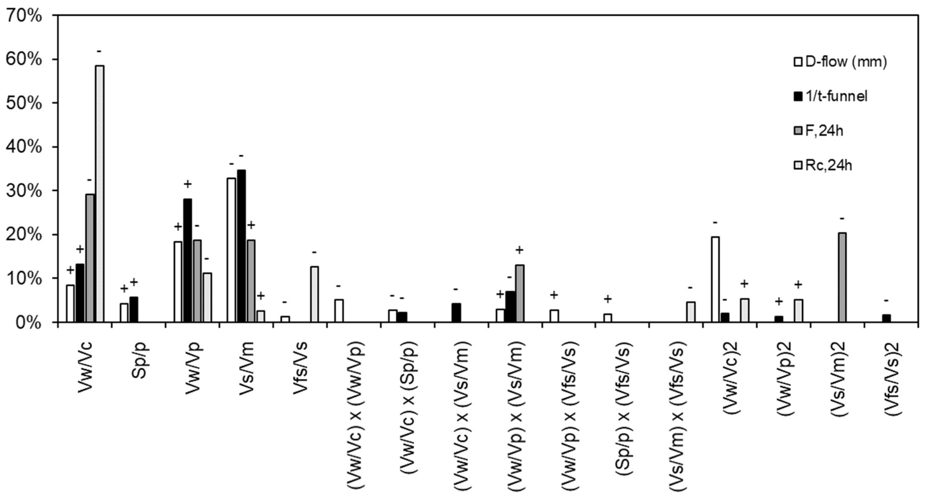
The final models (in terms of coded factors) are illustrated in Figure 8 regarding the relative impact of each factor by comparing the corresponding coefficient with the remaining (higher values of the estimated coefficient indicate the higher influence of the design variable in the response). The sign (positive or negative) of the estimated coefficient is marked on each bar’s label. We recall that a positive coefficient means that the response (or transformed response) variable will increase if the given mixture parameter increases and vice-versa.
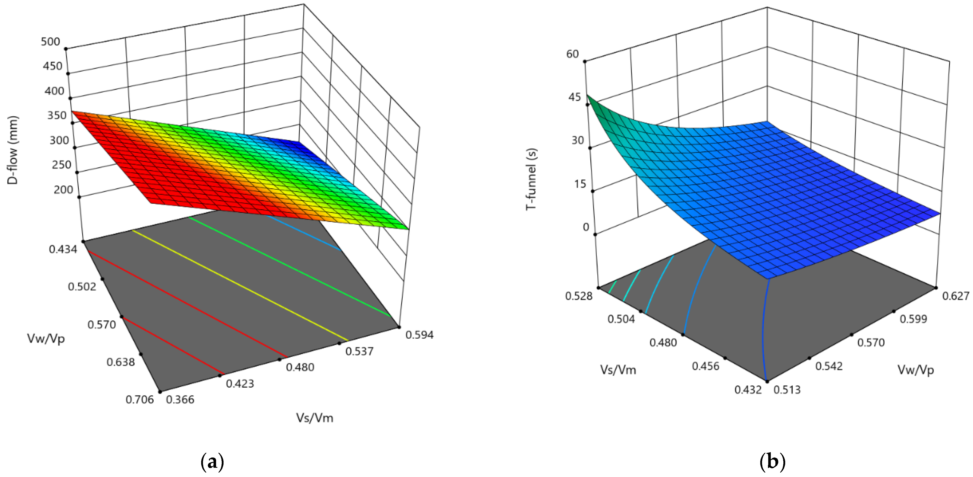
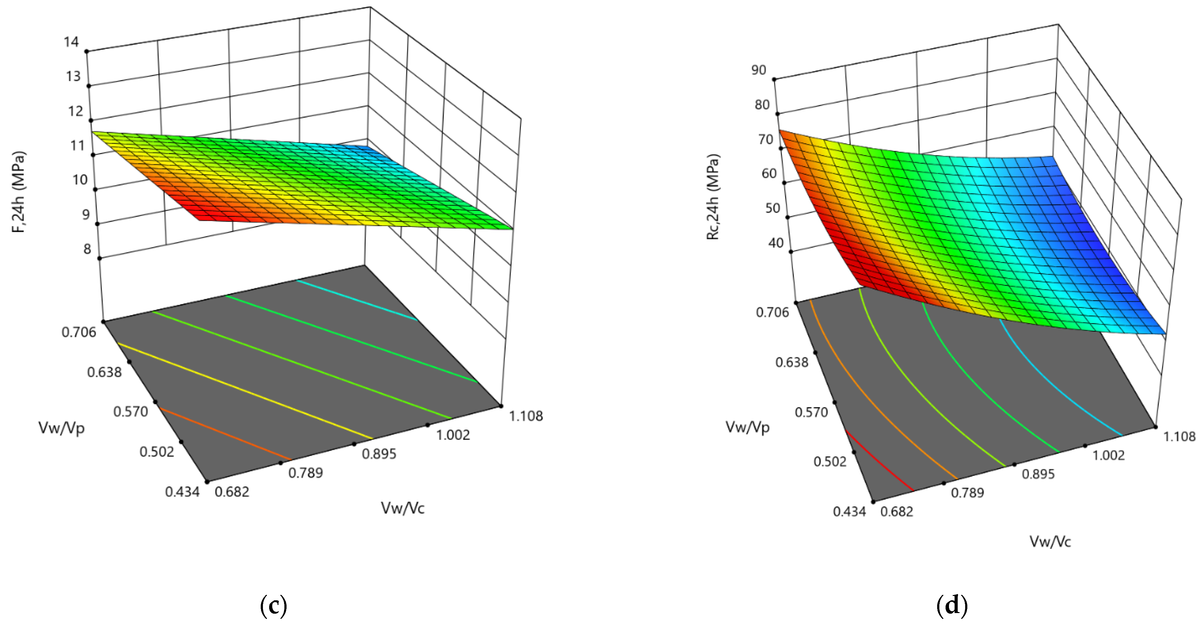
The response surfaces corresponding to the two main effects for each response of the mixtures are illustrated in Figure 9. For the D-flow and the T-funnel variation, the most significant factor is the volume of sand concerning the mortar (Vs/Vm) and the content of water/fines factors (Vw/Vp). In addition, it was possible to confirm the great influence of the water/cement factor (Vw/Vc) on the flexural (F,24 h) and compressive strength (Rc,24 h) of the mortars. In the order of inversely proportional influence, there is the fine sand concerning medium sand (Vfs/Vs) and the content of water/fines factors (Vw/Vp). The other factors have a smaller influence on the responses, exhibiting smaller estimated coded coefficients.
3.8. Models Validation
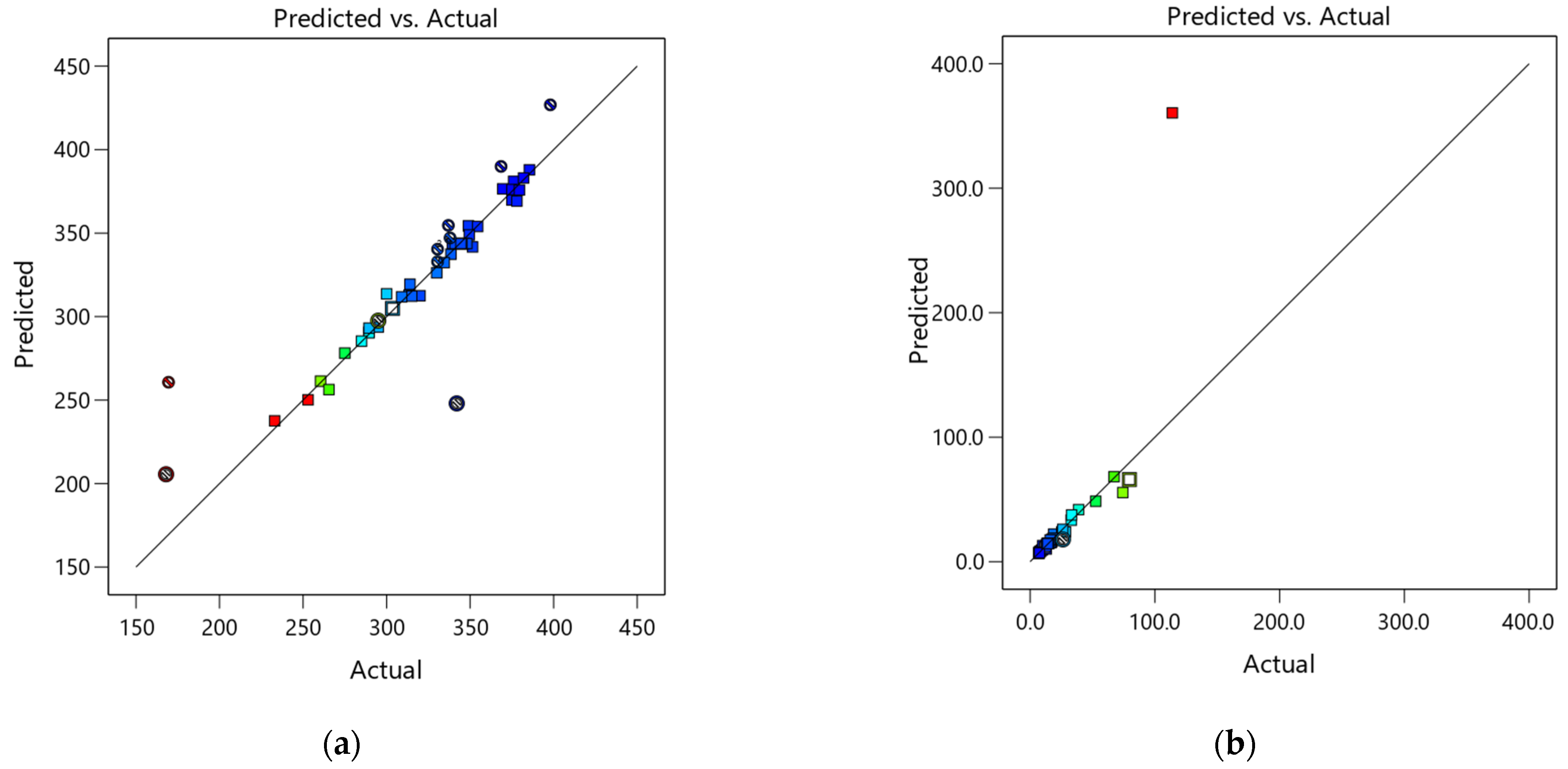
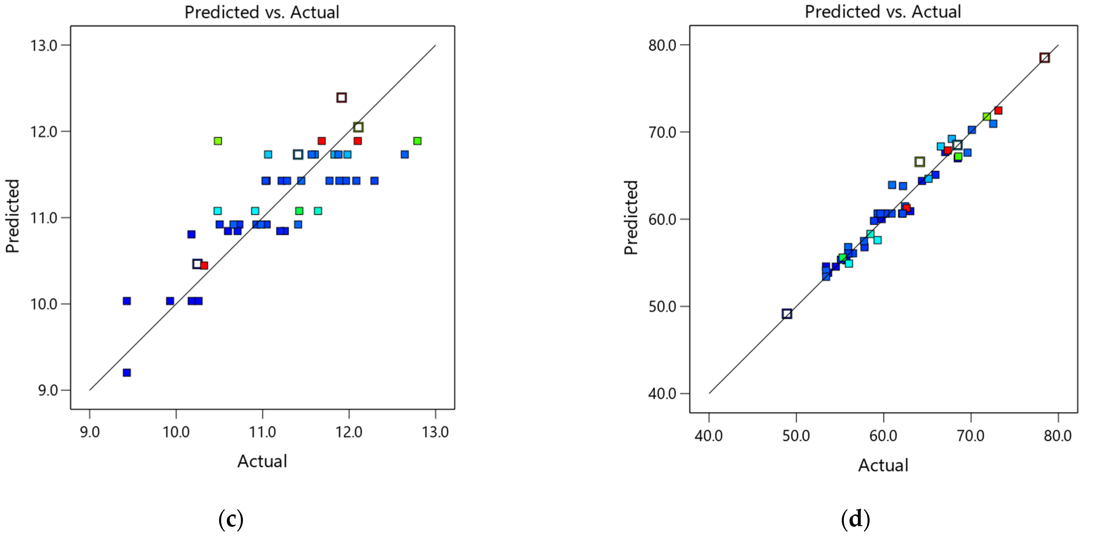
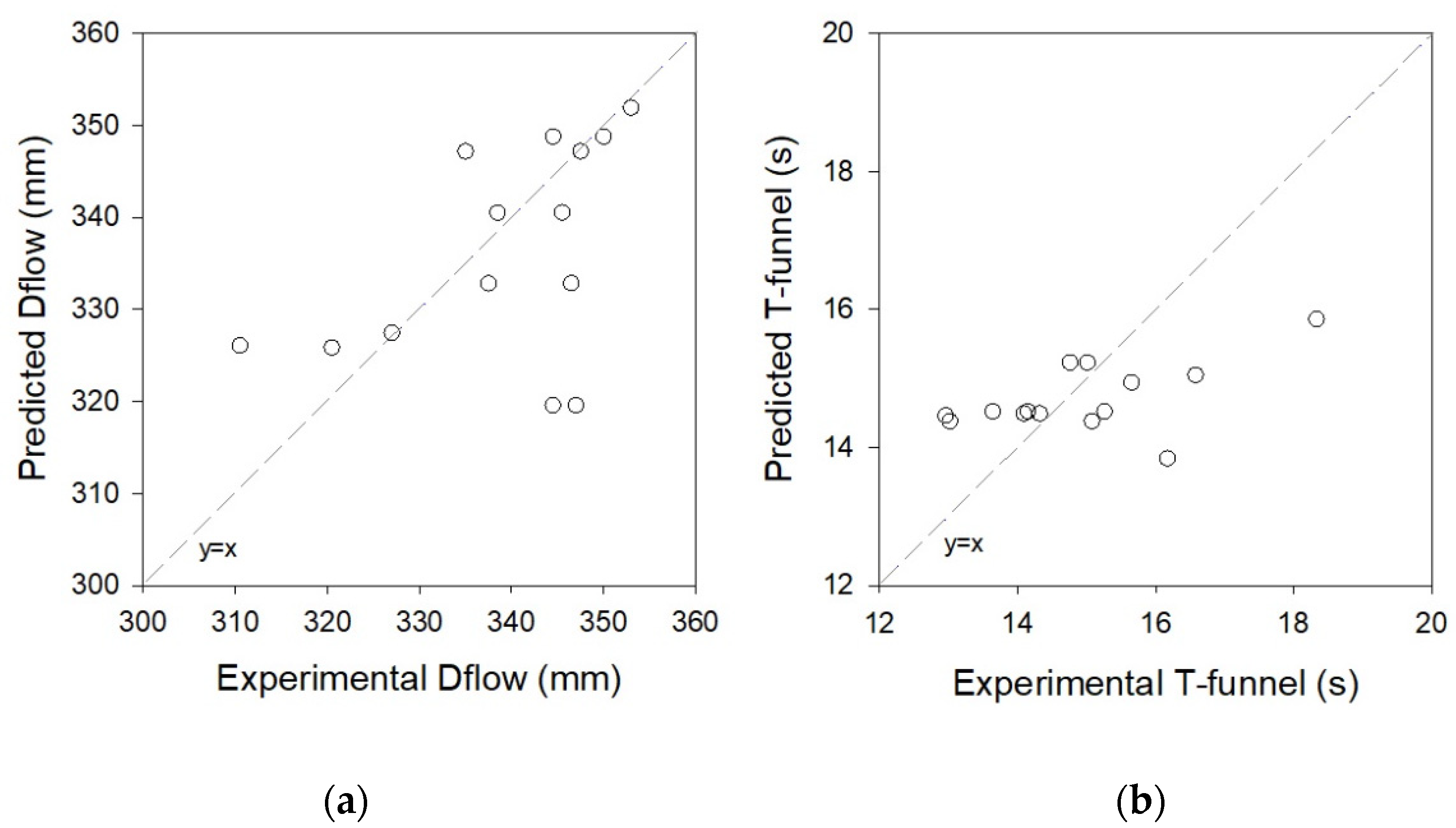
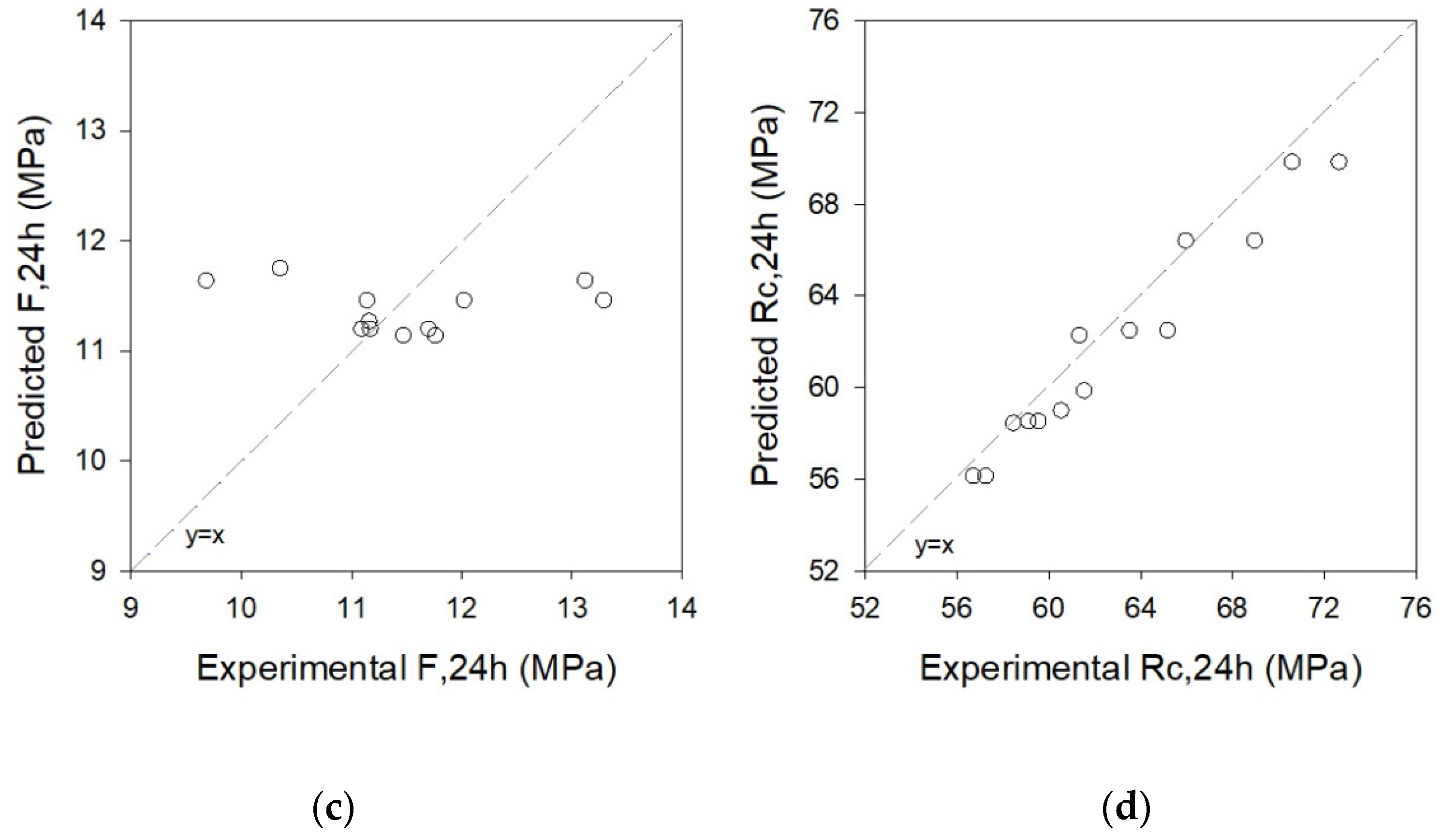
In order to validate the statistical models presented in Table 13, Maia [25] produced more than 14 SCHSCM mixtures and performed the experiments described in Section 2. The mixture proportion (in coded values) for these mixtures is presented in the last 14 lines of Table 3. The experimental results obtained and the estimated results given by the regression models are illustrated in Figure 11, including the x = y diagonals. The ratio between the predicted-to-measured values ranges from 0.84 to 1.20. The most accurate predictions are given by the Rc,24 h and D-flow models, where predicted-to-measured values range from 0.96 to 1.02 and 0.92 to 1.05, respectively. In addition, as expected, the flexural strength obtained results that exhibited higher dispersions when compared to the other results.
4. Optimisation
The empirical models obtained for modelling and predicting the relevant SCHSM properties were also used for mixture optimisation purposes. The optimisation module in Design-Expert studied in this paper searches for a combination of factor levels that simultaneously satisfy the goals established for each response and factor (see Table 14). The procedure uses the desirability function (D), and the solutions with D ≥ 0.995 were considered optimal. The optimisation was developed in two different scenarios, as follows in Section 4.1 and Section 4.2.
4.1. Self-Compacting Ability
The first optimisation scenario was to find mortar mixtures with self-compacting ability. The self-compacting ability was translated by targeting optimisation restrictions of a D-flow = 260 mm and a T-funnel = 10 s. This optimisation problem is defined in the second column of Table 14 and is entitled “self-compacting ability”. The importance level for all constraints, both mixture parameters and response variables, was kept the same. The optimisation aimed only to obtain solutions within the CCD region. Thus, the constraint conditions for mixture parameters were “In CCD range”.
In total, 68 mixture SCHSM solutions were found with D ≥ 0.995 in the region ; ; ; ; and .
4.2. SCC with High Early Strength
The second optimisation scenario was intended to discover self-compacting and high early strength mixtures simultaneously (see the third column of Table 14, entitled “self-compacting ability and high early strength”). For that, the optimisation conditions were: D-flow in the range from 259 to 261 mm, T-funnel in the range from 9.8 to 10.2 s, and compressive strength higher than 50 MPa at 24 h. The importance level for all constraints, both mixture parameters and response variables were kept the same. The optimisation aimed only to obtain solutions within the CCD region; thus, the constraint conditions for mixture parameters were “In CCD range”.
The best combination of SCHSM mixture parameters was: Vc/Vp = 1.098; sp/p = 0.0243; Vw/Vp = 0.607; Vs/Vm = 0.478; and Vfs/vs = 0.047. The corresponding estimated properties and their 95% confidence interval are presented in Table 15.
5. Conclusions
The current study investigates the effect of SCHSCM mixture design variables. It selects the best combination of powder materials (in a binary mixture of Portland cement + MTCK), water/binder ratio, superplasticiser dosage, and aggregates to reach optimum values of self-compactability and high early-age strength. As such, the DoE approach was followed to obtain regression models that could describe and predict the relevant engineering properties. In addition, regression models were used for optimisation purposes. The following main conclusions were drawn:
- -
- Regression models were found to be adequate to describe SCHSCM properties over the experimental region, namely, slump-flow diameter, T-funnel time, and flexural and compressive strength at 24 h;
- -
- The Vs/Vm factor exhibited the strongest (negative) effect on the slump-flow diameter and T-funnel time;
- -
- The Vw/Vp factor was found to have the most significant effect on mechanical strength, corresponding to response variables F,24 h and Rc,24 h;
- -
- Vw/Vc was the second most influencing factor, with a positive effect on the slump-flow diameter and T-funnel time and a negative effect on F,24 h and Rc,24 h;
- -
- The variation of Sp/p used in the current CCD was small compared to the remaining factors. As such, Sp/p exhibited the lowest influence on SCHSCM properties when compared to other mixture parameters;
- -
- The proposed optimal mixture represented the best compromise between self-compacting ability—a flow diameter of 250 mm and funnel time equal to 10 s—and a compressive strength higher than 50 MPa at 24 h without any special curing treatment and was found for Vc/Vp = 1.098; sp/p = 0.0243; Vw/Vp = 0.607; Vs/Vm = 0.478; and Vfs/vs = 0.047.
Even though transposing the mortar study into SCC is out of the scope of the manuscript, SCC mixtures can be obtained by fixing the mortar mix proportions given in Section 4.2 and adding a coarse aggregate. However, tests on the concrete level are needed to optimise the aggregate skeleton. Moreover, based on regression models, contour plots or interaction diagrams can be computed and simplify the test protocol required to optimise a given SCC mixture, namely, to select the combination of powder materials with admixtures. In particular, they can help to compare the efficiency of different admixtures and alternative SCM. Optimised mortar mixtures can serve as reference mixtures in a quality control plan to detect variations in different deliveries of constituent materials, such as cement, filler, or superplasticiser. The derived models can also be useful to predict mortar properties when the material properties change, such as the cement source.
The procedure presented in this work can easily be implemented in any concrete laboratory of a production centre since it involves mortar tests which are easy to carry out with simple tests and equipment.
Author Contributions
Conceptualisation, N.C., A.M.M., P.M.-O. and L.M.; methodology, N.C, A.M.M., P.M.-O. and L.M.; software, N.C., A.M.M., P.M.-O. and L.M.; validation, A.M.M., P.M.-O. and L.M.; formal analysis, N.C., A.M.M., P.M.-O. and L.M.; investigation, N.C. and L.M.; resources, L.M.; data curation, A.M.M. and L.M.; writing—original draft preparation, N.C., A.M.M. and P.M.-O.; writing—review and editing, N.C., A.M.M., P.M.-O. and L.M.; visualisation, N.C., A.M.M., P.M.-O. and L.M.; supervision, A.M.M. and L.M.; project administration, A.M.M. and L.M.; funding acquisition, A.M.M. and L.M. All authors have read and agreed to the published version of the manuscript.
Funding
This work is funded by: Base Funding—UIDB/04708/2020 of the CONSTRUCT—Instituto de I&D em Estruturas e Construções—funded by national funds through the FCT/MCTES (PIDDAC); by the national funds through FCT, Fundação para a Ciência e a Tecnologia, I.P., under the Scientific Employment Stimulus (Institutional Call, CEECINST/00049/2018); and the national funds through FCT, Fundação para a Ciência e a Tecnologia, I.P., under individual Scientific Employment Stimulus 2021.01765.CEECIND. The author Paula Milheiro-Oliveira was partially supported by CMUP, a member of LASI, which is financed by national funds through FCT—Fundação para a Ciência e a Tecnologia, I.P., under the project with reference UIDB/00144/2020.
Institutional Review Board Statement
Not applicable.
Informed Consent Statement
Not applicable.
Data Availability Statement
Acknowledgments
Collaboration and materials supply by Secil, Omya Comital and Sika is gratefully acknowledged.
Conflicts of Interest
The authors declare no conflict of interest.
Abbreviations
| ANOVA | Analysis Of Variance |
| CCD | Central Composite Design |
| Ci | Central points of CCD |
| CCi | Axial points of CCD |
| d | Days |
| D | Desirability function |
| D-flow | Flow Diameter (mm) |
| DoE | Design of Experiments |
| F,24 h | Flexure strength at 24 h (MPa) |
| Fi | Factorial points of CCD |
| GDP | Gross Domestic Product |
| GHG | Greenhouse Gas |
| h | Hours |
| LF | Limestone Filler |
| p | Powder Mass |
| PC | Portland Cement |
| PSD | Particle Size Distribution |
| Rc,24 h | Compressive strength at 24 h (MPa) |
| SCC | Self-Compacting Concrete |
| SCHSCM | Self-Compacting High early Strength Cement-based Mortars |
| SCM | Supplementary Cementitious Materials |
| SDG | Sustainable Development Goals |
| Sp | Superplasticizer |
| Sp/p | Superplasticiser to powder mass ratio |
| RH | Relative Humidity (%) |
| T-funnel | Funnel Time |
| Vc | Cement Volume |
| VC | Vibrated Concrete |
| Vi | Validation points |
| Vfs | Fine Sand Volume |
| VIF | Value of the Inflammation Factor |
| Vm | Mortar Volume |
| Vp | Powder Volume |
| Vs | Sand Volume |
| Vw | Water Volume |
| Vw/Vc | Water to cement volume ratio |
| Vw/Vp | Water to powder volume ratio |
| Vs/Vm | Sand to mortar volume ratio |
| Vfs/Vs | Fine sand to total sand volume ratio |
References
- Omer, M.A.B.; Noguchi, T. A conceptual framework for understanding the contribution of building materials in the achievement of Sustainable Development Goals (SDGs). Sustain. Cities Soc. 2020, 52, 101869. [Google Scholar] [CrossRef]
- Antiohos, S.K.; Tapali, J.G.; Zervaki, M.; Sousa-Coutinho, J.; Tsimas, S.; Papadakis, V.G. Low embodied energy cement containing untreated RHA: A strength development and durability study. Constr. Build. Mater. 2013, 49, 455–463. [Google Scholar] [CrossRef]
- Nunes, S.; Matos, A.M.; Duarte, T.; Figueiras, H.; Sousa-Coutinho, J. Mixture design of self-compacting glass mortar. Cem. Concr. Compos. 2013, 43, 1–11. [Google Scholar] [CrossRef]
- Matos, A.M. Design of Eco-Efficient Ultra-High Performance Fibre Reinforced Cement-Based Composite for Rehabilitation/Strengthening Applications; University of Porto: Porto, Portugal, 2020. [Google Scholar]
- Okamura, H.; Ouchi, M. Self-Compacting Concrete. J. Adv. Concr. Technol. 2003, 1, 5–15. [Google Scholar] [CrossRef]
- Nunes, S.; Figueiras, H.; Milheiro Oliveira, P.; Coutinho, J.S.; Figueiras, J. A methodology to assess robustness of SCC mixtures. Cem. Concr. Res. 2006, 36, 2115–2122. [Google Scholar] [CrossRef]
- Yogitha, B.; Karthikeyan, M.; Muni Reddy, M.G. Progress of sugarcane bagasse ash applications in production of Eco-Friendly concrete—Review. Mater. Today Proc. 2020, 33, 695–699. [Google Scholar] [CrossRef]
- Gettu, R.; Pillai, R.G.; Santhanam, M.; Dhanya, B.S. Ways of Improving the Sustainability of Concrete Technology Through the Effective Use of Admixtures. Indian Inst. Technol. Madras Chennai 2018, 21. [Google Scholar]
- Loganayagan, S.; Chandra Mohan, N.; Dhivyabharathi, S. Sugarcane bagasse ash as alternate supplementary cementitious material in concrete. Mater. Today Proc. 2021, 45, 1004–1007. [Google Scholar] [CrossRef]
- Wagner, J.R.; Mount, E.M.; Giles, H.F. Design of Experiments. In Extrusion; William Andrew Publishing: Norwich, NY, USA, 2014; pp. 291–308. ISBN 978-1-4377-3481-2. [Google Scholar]
- Shi, C.; Wu, Z.; Lv, K.; Wu, L. A review on mixture design methods for self-compacting concrete. Constr. Build. Mater. 2015, 84, 387–398. [Google Scholar] [CrossRef]
- Khayat, K.H.; Ghezal, A.; Hadriche, M.S. Utility of statistical models in proportioning self-consolidating concrete. Mater. Struct. 2000, 33, 338–344. [Google Scholar] [CrossRef]
- Nunes, S.; Costa, C. Self-compacting concrete also standing for sustainable circular concrete. In Waste and Byproducts in Cement-Based Materials; Woodhead Publishing: Sawston, UK, 2021; pp. 439–480. [Google Scholar]
- Matos, A.M.; Maia, L.; Nunes, S.; Milheiro-Oliveira, P. Design of self-compacting high-performance concrete: Study of mortar phase. Constr. Build. Mater. 2018, 167, 617–630. [Google Scholar] [CrossRef]
- Dinakar, P. Design of self-compacting concrete with fly ash. Mag. Concr. Res. 2012, 64, 401–409. [Google Scholar] [CrossRef]
- Rojo-López, G.; Nunes, S.; González-Fonteboa, B.; Martínez-Abella, F. Quaternary blends of portland cement, metakaolin, biomass ash and granite powder for production of self-compacting concrete. J. Clean. Prod. 2020, 266, 121666. [Google Scholar] [CrossRef]
- Ghosh, D.; Abd-Elssamd, A.; Ma, Z.J.; Hun, D. Development of high-early-strength fiber-reinforced self-compacting concrete. Constr. Build. Mater. 2021, 266, 121051. [Google Scholar] [CrossRef]
- Al-Alaily, H.S.; Hassan, A.A.A. Refined statistical modeling for chloride permeability and strength of concrete containing metakaolin. Constr. Build. Mater. 2016, 114, 564–579. [Google Scholar] [CrossRef]
- Abouhussien, A.A.; Hassan, A.A.A. Optimising the durability and service life of self-consolidating concrete containing metakaolin using statistical analysis. Constr. Build. Mater. 2015, 76, 297–306. [Google Scholar] [CrossRef]
- Abouhussien, A.A.; Hassan, A.A.A. Application of Statistical Analysis for Mixture Design of High-Strength Self-Consolidating Concrete Containing Metakaolin. J. Mater. Civ. Eng. 2014, 26, 04014016. [Google Scholar] [CrossRef]
- Dvorkin, L.; Bezusyak, A.; Lushnikova, N.; Ribakov, Y. Using mathematical modeling for design of self compacting high strength concrete with metakaolin admixture. Constr. Build. Mater. 2012, 37, 851–864. [Google Scholar] [CrossRef]
- Matos, A.M.; Nunes, S.; Costa, C.; Barroso-Aguiar, J.L. Spent equilibrium catalyst as internal curing agent in UHPFRC. Cem. Concr. Compos. 2019, 104, 103362. [Google Scholar] [CrossRef]
- Nunes, S. Performance-Based Design of Self-Compacting Concrete (SCC): A Contribution to Enchance SCC Mixtures Robustness; Faculty of Enginnering of University of Porto: Porto, Portugal, 2008. [Google Scholar]
- Galobardes, I.; Salvador, R.P.; Cavalaro, S.H.P.; Figueiredo, A.; Goodier, C.I. Adaptation of the standard EN 196-1 for mortar with accelerator. Constr. Build. Mater. 2016, 127, 125–136. [Google Scholar] [CrossRef] [Green Version]
- Maia, L. Experimental dataset from a central composite design to develop mortars with self-compacting properties and high early age strength. Data Brief 2021, 39, 107563. [Google Scholar] [CrossRef] [PubMed]
- EFNARC. Specification and Guidelines for Self-Compacting Concrete; EFNARC: Farnham, UK, 2002. [Google Scholar]
- NP EN 196-1—Methods of Testing Cement. Part 1: Determination of Strength; Instituto Português da Qualidade: Lisbon, Portugal, 2006; pp. 1–37. [Google Scholar]
- De Barros Neto, B.; Scarminio, I.S.; Bruns, R.E. Como Fazer Experimentos, 4th ed.; Bookman, Ed.; Artmed Editora SA: Porto Alegre, Brazil, 2010; ISBN 978-85-7780-652-2. [Google Scholar]
- Montgomery, D.C. Introduction to Statistical Quality Control, 7th ed.; John Wiley and Sons Inc.: Hoboken, NJ, USA, 2013; ISBN 978-1-118-14681-1. [Google Scholar]
Figure 1.
Mixture proportions of OVC and SCC (in % volume).

Figure 2.
(a) Normal probability plot of the externally studentised residuals for the D-flow fitted model, and (b) plot of the externally studentised residuals versus D-flow predicted values.
Figure 2.
(a) Normal probability plot of the externally studentised residuals for the D-flow fitted model, and (b) plot of the externally studentised residuals versus D-flow predicted values.

Figure 3.
T-funnel results: F15 excluded (arrow).

Figure 4.
(a) Normal probability plot of the externally studentised residuals for the T-funnel fitted model, and (b) plot of the externally studentised residuals versus T-funnel fitted values.
Figure 4.
(a) Normal probability plot of the externally studentised residuals for the T-funnel fitted model, and (b) plot of the externally studentised residuals versus T-funnel fitted values.

Figure 5.
(a) Normal probability plot of the externally studentised residuals for the F,24 h fitted model, and (b) plot of the externally studentised residuals versus F,24 h fitted values.
Figure 5.
(a) Normal probability plot of the externally studentised residuals for the F,24 h fitted model, and (b) plot of the externally studentised residuals versus F,24 h fitted values.

Figure 6.
(a) Normal probability plot of the externally studentised residuals for the Rc,24 h fitted model, and (b) plot of the externally studentised residuals versus Rc,24 h fitted values.
Figure 6.
(a) Normal probability plot of the externally studentised residuals for the Rc,24 h fitted model, and (b) plot of the externally studentised residuals versus Rc,24 h fitted values.

Figure 7.
Rc,24 h: (a) Cook’s distance and (b) leverage.

Figure 8.
Influence of each factor on fresh state responses, in which (+) Positive effect in response models; (−) Negative effect in response model (see Table 13).
Figure 8.
Influence of each factor on fresh state responses, in which (+) Positive effect in response models; (−) Negative effect in response model (see Table 13).

Figure 9.
Effect of the Vs/Vm and Vw/Vp ratios on (a) D-flow and (b) T-funnel; effect of Vw/Vc and Vw/Vp on (c) F,24 h and (d) Rc,24 h.
Figure 9.
Effect of the Vs/Vm and Vw/Vp ratios on (a) D-flow and (b) T-funnel; effect of Vw/Vc and Vw/Vp on (c) F,24 h and (d) Rc,24 h.


Figure 10.
Predicted versus actual plan: (a) D-flow, (b) T-funnel, (c) F,24 h, and (d) Rc,24 h.


Figure 11.
Predicted versus measured: (a) D-flow; (b) T-funnel; (c) F,24 h, and (d) Rc,24 h.


Table 1.
Correspondence between the coded values and actual values of the design variables.
| Design Variables | −2.378 | −1 | 0 | +1 | +2.378 |
|---|---|---|---|---|---|
| X1: Vw/Vc | 0.682 | 0.805 | 0.895 | 0.894 | 1.108 |
| X2: Sp/p | 0.019 | 0.022 | 0.024 | 0.025 | 0.029 |
| X3: Vw/Vp | 0.434 | 0.513 | 0.570 | 0.627 | 0.706 |
| X4: Vs/Vm | 0.366 | 0.432 | 0.480 | 0.528 | 0.594 |
| X5: Vfs/Vs | 0.043 | 0.250 | 0.400 | 0.550 | 0.757 |
Table 2.
Response variable summary.
| Response Variables | Units | Measurement Method |
|---|---|---|
| Y1: D-flow | mm | EFNARC |
| Y2: T-funnel | s | EFNARC |
| Y3: F,24 h | MPa | EN 196-1 |
| Y4: Rc,24 h | MPa | EN-196-1 |
Table 3.
The mixture proportion (coded values) and experimental results obtained by Maia [25] and used for model fitting and validation points.
Table 3.
The mixture proportion (coded values) and experimental results obtained by Maia [25] and used for model fitting and validation points.
| CCD Point | Coded Values | Results | |||||||
|---|---|---|---|---|---|---|---|---|---|
| Vw/Vc | Sp/p | Vw/Vp | Vs/Vm | Vfs/Vs | D-Flow | T-Funnel | F,24 h | Rc,24 h | |
| (mm) | (s) | (MPa) | (MPa) | ||||||
| C1 | 0.00 | 0.00 | 0.00 | 0.00 | 0.00 | 346.50 | 14.98 | 11.77 | 59.89 |
| C2 | 0.00 | 0.00 | 0.00 | 0.00 | 0.00 | 346.00 | 13.77 | 12.29 | 62.10 |
| C3 | 0.00 | 0.00 | 0.00 | 0.00 | 0.00 | 339.50 | 14.15 | 11.28 | 59.31 |
| C4 | 0.00 | 0.00 | 0.00 | 0.00 | 0.00 | 348.00 | 14.74 | 12.08 | 60.90 |
| C5 | 0.00 | 0.00 | 0.00 | 0.00 | 0.00 | 339.50 | 14.53 | 11.96 | 60.00 |
| C6 | 0.00 | 0.00 | 0.00 | 0.00 | 0.00 | 341.00 | 14.38 | 11.89 | 62.17 |
| C7 | 0.00 | 0.00 | 0.00 | 0.00 | 0.00 | 345.00 | 13.56 | 11.05 | 60.18 |
| C8 | 0.00 | 0.00 | 0.00 | 0.00 | 0.00 | 344.50 | 14.23 | 11.03 | 59.63 |
| F1 | −1.00 | −1.00 | −1.00 | −1.00 | −1.00 | 330.00 | 18.89 | 11.60 | 72.54 |
| F2 | 1.00 | −1.00 | −1.00 | −1.00 | −1.00 | 349.00 | 12.26 | 11.05 | 57.80 |
| F3 | −1.00 | 1.00 | −1.00 | −1.00 | −1.00 | 338.50 | 16.70 | 12.64 | 70.09 |
| F4 | 1.00 | 1.00 | −1.00 | −1.00 | −1.00 | 354.50 | 11.32 | 10.50 | 56.06 |
| F5 | −1.00 | −1.00 | 1.00 | −1.00 | −1.00 | 375.00 | 9.24 | 11.26 | 67.05 |
| F6 | 1.00 | −1.00 | 1.00 | −1.00 | −1.00 | 369.50 | 7.08 | 9.43 | 55.72 |
| F7 | −1.00 | 1.00 | 1.00 | −1.00 | −1.00 | 376.00 | 7.80 | 10.60 | 68.47 |
| F8 | 1.00 | 1.00 | 1.00 | −1.00 | −1.00 | 375.00 | 6.91 | 10.18 | 53.40 |
| F9 | −1.00 | −1.00 | −1.00 | 1.00 | −1.00 | 253.00 | 114.06 | 11.68 | 73.13 |
| F10 | 1.00 | −1.00 | −1.00 | 1.00 | −1.00 | 289.50 | 38.91 | 11.64 | 58.49 |
| F11 | −1.00 | 1.00 | −1.00 | 1.00 | −1.00 | 260.50 | 74.32 | 10.48 | 71.81 |
| F12 | 1.00 | 1.00 | −1.00 | 1.00 | −1.00 | 289.50 | 33.03 | 10.91 | 59.30 |
| F13 | −1.00 | −1.00 | 1.00 | 1.00 | −1.00 | 295.00 | 25.40 | 11.83 | 67.80 |
| F14 | 1.00 | −1.00 | 1.00 | 1.00 | −1.00 | 313.50 | 17.53 | 11.41 | 55.93 |
| F15 | −1.00 | 1.00 | 1.00 | 1.00 | −1.00 | 303.50 | 26.33 | 11.41 | 68.43 |
| F16 | 1.00 | 1.00 | 1.00 | 1.00 | −1.00 | 320.00 | 14.15 | 10.93 | 56.48 |
| F17 | −1.00 | −1.00 | −1.00 | −1.00 | 1.00 | 300.00 | 28.43 | 11.06 | 66.54 |
| F18 | 1.00 | −1.00 | −1.00 | −1.00 | 1.00 | 351.50 | 12.89 | 10.69 | 55.93 |
| F19 | −1.00 | 1.00 | −1.00 | −1.00 | 1.00 | 334.50 | 17.67 | 11.57 | 69.59 |
| F20 | 1.00 | 1.00 | −1.00 | −1.00 | 1.00 | 349.50 | 11.73 | 10.73 | 55.10 |
| F21 | −1.00 | −1.00 | 1.00 | −1.00 | 1.00 | 378.00 | 9.90 | 11.20 | 65.92 |
| F22 | 1.00 | −1.00 | 1.00 | −1.00 | 1.00 | 379.50 | 7.16 | 9.93 | 54.52 |
| F23 | −1.00 | 1.00 | 1.00 | −1.00 | 1.00 | 385.50 | 8.54 | 10.71 | 64.39 |
| F24 | 1.00 | 1.00 | 1.00 | −1.00 | 1.00 | 382.00 | 6.94 | 10.26 | 53.64 |
| F25 | −1.00 | −1.00 | −1.00 | 1.00 | 1.00 | 233.00 | * | 12.10 | 67.34 |
| F26 | 1.00 | −1.00 | −1.00 | 1.00 | 1.00 | 275.00 | 52.64 | 11.42 | 55.30 |
| F27 | −1.00 | 1.00 | −1.00 | 1.00 | 1.00 | 265.50 | 67.34 | 12.79 | 68.54 |
| F28 | 1.00 | 1.00 | −1.00 | 1.00 | 1.00 | 285.00 | 33.30 | 10.48 | 56.02 |
| F29 | −1.00 | −1.00 | 1.00 | 1.00 | 1.00 | 289.50 | 26.20 | 11.98 | 65.12 |
| F30 | 1.00 | −1.00 | 1.00 | 1.00 | 1.00 | 315.00 | 16.51 | 10.98 | 53.39 |
| F31 | −1.00 | 1.00 | 1.00 | 1.00 | 1.00 | 309.00 | 18.57 | 11.88 | 60.96 |
| F32 | 1.00 | 1.00 | 1.00 | 1.00 | 1.00 | 314.00 | 17.07 | 10.66 | 53.41 |
| CC1 | −2.38 | 0.00 | 0.00 | 0.00 | 0.00 | 168.00 | * | 11.91 | 78.42 |
| CC2 | 2.38 | 0.00 | 0.00 | 0.00 | 0.00 | 342.00 | 11.55 | 10.25 | 48.92 |
| CC3 | 0.00 | −2.38 | 0.00 | 0.00 | 0.00 | 330.50 | 17.64 | 11.45 | 62.44 |
| CC4 | 0.00 | 2.38 | 0.00 | 0.00 | 0.00 | 337.00 | 12.71 | 11.22 | 58.89 |
| CC5 | 0.00 | 0.00 | −2.38 | 0.00 | 0.00 | 295.00 | 79.63 | 12.11 | 64.13 |
| CC6 | 0.00 | 0.00 | 2.38 | 0.00 | 0.00 | 368.50 | 7.27 | 10.18 | 63.04 |
| CC7 | 0.00 | 0.00 | 0.00 | −2.38 | 0.00 | 398.00 | 7.49 | 9.43 | 59.77 |
| CC8 | 0.00 | 0.00 | 0.00 | 2.38 | 0.00 | 169.50 | * | 10.32 | 62.62 |
| CC9 | 0.00 | 0.00 | 0.00 | 0.00 | −2.38 | 338.00 | 16.55 | Na | 62.21 |
| CC10 | 0.00 | 0.00 | 0.00 | 0.00 | 2.38 | 330.50 | 16.14 | Na | 57.75 |
| V1 | 0.63 | 3.05 | 0.21 | 0.52 | −2 | 16.17 | 320.50 | 11.70 | 58.45 |
| V2 | 0.63 | 1.5 | 0.21 | 0.52 | −2 | 16.58 | 327.00 | 11.09 | 60.53 |
| V3 | 0.63 | 1.5 | 0.21 | 0.52 | −2.67 | 18.33 | 310.50 | 11.17 | 61.54 |
| V4 | −0.13 | 0.21 | −0.66 | −0.62 | 0.00 | 12.96 | 353.00 | 12.02 | 61.33 |
| V5 | 1.08 | −0.42 | −1.13 | −0.62 | 0.00 | 14.09 | 337.50 | 11.47 | 56.70 |
| V6 | −1.34 | 0.52 | −0.14 | −0.62 | 0.00 | 14.15 | 347.00 | 10.35 | 70.59 |
| V7 | −0.82 | 0.58 | −0.39 | −0.62 | 0.00 | 13.64 | 338.50 | 9.68 | 65.96 |
| V8 | 0.57 | −0.15 | −0.92 | −0.62 | 0.00 | 13.02 | 335.00 | 11.16 | 59.11 |
| V9 | −0.13 | −0.42 | −0.66 | −0.62 | 0.00 | 14.76 | 350.00 | 13.29 | 63.51 |
| V10 | −0.13 | −0.42 | −0.66 | −0.62 | 0.00 | 15.01 | 344.50 | 11.14 | 65.16 |
| V11 | 1.08 | −0.42 | −1.13 | −0.62 | 0.00 | 14.32 | 346.50 | 11.76 | 57.25 |
| V12 | −1.34 | 0.52 | −0.14 | −0.62 | 0.00 | 15.65 | 344.50 | 13.97 | 72.63 |
| V13 | −0.82 | 0.58 | −0.39 | −0.62 | 0.00 | 15.26 | 345.50 | 13.12 | 68.96 |
| V14 | 0.57 | −0.15 | −0.92 | −0.62 | 0.00 | 15.08 | 347.50 | Na | 59.54 |
* impossible to measure; Na—non-available result.
Table 4.
The main statistics for all CCD points and central points.
| D-Flow (mm) | T-Funnel (s) | F,24 h (MPa) | Rc,24 h (MPa) | |
|---|---|---|---|---|
| All 50 mixtures | ||||
| Minimum | 168.00 | 6.91 | 9.43 | 48.92 |
| Maximum | 398.00 | 114.06 | 12.79 | 78.42 |
| Mean | 323.31 | 22.39 | 11.17 | 61.61 |
| Standard deviation | 48.97 | 21.63 | 0.77 | 6.24 |
| Coefficient of variation (%) | 15.15 | 96.62 | 6.93 | 10.14 |
| Central points (Ci) | ||||
| Minimum | 339.50 | 13.56 | 11.03 | 59.31 |
| Maximum | 348.00 | 14.98 | 12.29 | 62.17 |
| Mean | 343.75 | 14.29 | 11.67 | 60.52 |
| Standard deviation | 3.31 | 0.47 | 0.48 | 1.10 |
| Coefficient of variation (%) | 0.96 | 3.31 | 4.16 | 1.81 |
Table 13.
Final equations in terms of actual factors: estimated coefficients.
| Model Terms | D-Flow (mm) | 1/(T-Funnel) (s) | F,24 h (MPa) | Rc,24 h (MPa) |
|---|---|---|---|---|
| Independent | −2154.81 | −1.3582 | 5.400 | 293.77 |
| Vw/Vc | 5375.51 | 1.2092 | −4.529 | −257.75 |
| Sp/p | 15,060.05 | 13.4743 | - | −186.47 |
| Vw/Vp | 1141.35 | 1.1255 | −36.616 | −289.80 |
| Vs/Vm | −1375.32 | 1.4119 | 85.487 | 32.94 |
| Vfs/Vs | −365.99 | 0.0374 | - | −7.31 |
| (Vw/Vc) × (Vw/Vp) | −1050.80 | - | - | 85.43 |
| (Vw/Vc) × (Sp/p) | −17,105.24 | −12.0954 | - | - |
| (Vw/Vc) × (Vs/Vm) | 723.96 | −0.8550 | - | - |
| (Vw/Vp) × (Vs/Vm) | - | −2.2390 | 66.741 | - |
| (Vw/Vp) × (Vfs/Vs) | 349.05 | - | - | 35.06 |
| (Sp/p) × (Vfs/Vs) | 6673.75 | - | - | - |
| (Vs/Vm) × (Vfs/Vs) | - | - | - | −68.53 |
| (Vw/Vc)2 | −2581.92 | −0.2148 | - | 70.43 |
| (Vw/Vp)2 | - | 0.3375 | - | 168.84 |
| (Vs/Vm)2 | - | - | −123.018 | - |
| (Vfs/Vs)2 | - | −0.0602 | - | - |
Table 14.
Optimisation criteria.
| Self-Compacting Ability | Self-Compacting Ability and High Early Strength | |
|---|---|---|
| Constraints for optimisation | ||
| Mixture parameters: | ||
| Vw/Vc | In CCD range | In CCD range |
| Sp/p | In CCD range | In CCD range |
| Vw/Vp | In CCD range | In CCD range |
| Vs/Vm | In CCD range | In CCD range |
| Vfs/Vs | In CCD range | In CCD range |
| Response Variables: | ||
| D-flow (mm) | Target 260 | In range {259, 261} |
| T-funnel (s) | Target 10 | In range {9.8, 10.2} |
| F,24 h (MPa) | None | None |
| Rc,24 h (MPa) | None | >50 |
Table 15.
Estimated SCHSM properties of the optimised mixture.
| Response | Predicted Results | 95% CI Low | 95% CI High |
|---|---|---|---|
| D-flow | 259.15 | 237.78 | 280.51 |
| T-funnel | 9.87 | 9.1 | 10.79 |
| F,24 h | 10.31 | 9.93 | 10.7 |
| Rc,24 h | 50.00 | 46.86 | 53.14 |
Disclaimer/Publisher’s Note: The statements, opinions and data contained in all publications are solely those of the individual author(s) and contributor(s) and not of MDPI and/or the editor(s). MDPI and/or the editor(s) disclaim responsibility for any injury to people or property resulting from any ideas, methods, instructions or products referred to in the content. |
© 2023 by the authors. Licensee MDPI, Basel, Switzerland. This article is an open access article distributed under the terms and conditions of the Creative Commons Attribution (CC BY) license (https://creativecommons.org/licenses/by/4.0/).
Share and Cite
MDPI and ACS Style
Cangussu, N.; Matos, A.M.; Milheiro-Oliveira, P.; Maia, L. Numerical Design and Optimisation of Self-Compacting High Early-Strength Cement-Based Mortars. Appl. Sci. 2023, 13, 4142. https://doi.org/10.3390/app13074142
AMA Style
Cangussu N, Matos AM, Milheiro-Oliveira P, Maia L. Numerical Design and Optimisation of Self-Compacting High Early-Strength Cement-Based Mortars. Applied Sciences. 2023; 13(7):4142. https://doi.org/10.3390/app13074142
Chicago/Turabian StyleCangussu, Nara, Ana Mafalda Matos, Paula Milheiro-Oliveira, and Lino Maia. 2023. "Numerical Design and Optimisation of Self-Compacting High Early-Strength Cement-Based Mortars" Applied Sciences 13, no. 7: 4142. https://doi.org/10.3390/app13074142
Note that from the first issue of 2016, this journal uses article numbers instead of page numbers. See further details here.