Article

Chemical Characterization of PM2.5 at Rural and Urban Sites around the Metropolitan Area of Huancayo (Central Andes of Peru)

by
Alex Huamán De La Cruz
1,3,
Yessica Bendezu Roca
1,*,
Luis Suarez-Salas
2,
José Pomalaya
1,
Daniel Alvarez Tolentino
2 and
Adriana Gioda
3
1
Facultad de Ingeniería Química, Universidad Nacional del Centro del Perú (UNCP), Av. Mariscal Ramón Castilla N° 3909, El Tambo, Huancayo 12000, Peru
2
Instituto Geofísico del Perú (IGP), Calle Badajoz 169, Ate, Lima 15498, Peru
3
Department of Chemistry, Pontifical Catholic University of Rio de Janeiro (PUC-Rio), Rio de Janeiro 20000, Brazil
*
Author to whom correspondence should be addressed.
Atmosphere 2019, 10(1), 21; https://doi.org/10.3390/atmos10010021
Submission received: 4 December 2018 / Revised: 29 December 2018 / Accepted: 3 January 2019 / Published: 8 January 2019
(This article belongs to the Section Air Quality)

Abstract

:
The purpose of this study was to determine PM2.5 mass concentration and the contents of trace elements and water-soluble ions in samples collected inside the Metropolitan area of Huancayo. Four monitoring stations were installed at three urban areas (UNCP, HYO, and CHI) and one rural (IGP). The sampling campaign was carried out from March 2017 to November 2017. The PM2.5 content was determined by gravimetric method, and fifteen trace elements (TE) and seven water-soluble ions were detected by inductively coupled plasma mass spectrometry (ICP–MS), and ion chromatography (IC), respectively. Datasets were assessed by one ANOVA test to detect significant differences among monitoring station. Hierarchical cluster analysis (HCA) and principal component analysis (PCA) were applied for source identification. The mean annual concentration of PM2.5 mass concentrations has ranged (average) from 3.4 to 36.8 µg/m3 (16.6 ± 6.8 µg/m3) for the monitoring stations under study. The annual World Health Organization thresholds and national air quality standards were exceeded. Significant differences (p < 0.05) were observed between most trace elements at urban and rural areas. PCA and HCA illustrated that the most important sources of traces element originated of natural origin (soil re-suspension) and vehicular sources (fuel combustion, abrasion of vehicles tires, wear car components).

1. Introduction

Air pollution and atmospheric deposition of toxic trace elements have become a major environmental concern around the world because of its adverse effect on human health and the environment [1,2,3]. Among major urban air pollutants, airborne particulate matter (PM), in inhalable coarse particles (PM10—particles that have aerodynamic diameters less than or equal to 10 µm) or particularly fine particles (PM2.5—aerodynamic diameters of 2.5 µm or less) [4] show potential risk to the health human causing premature mortality and cardiovascular diseases [5]. Airborne particulate matter represents a complex mixture of organic and inorganic substances [6,7] such as chemical elements (i.e., Si, Al, Fe, Ca, Ti, V, Cr, Cu, Zn), volatile organic compounds (VOCs), water-soluble ions (i.e., SO 4 2 ,   NO 3 ,   NH 4 + , Na+, Ca2+, Mg2+, and K+) among others that can threaten living organisms and human health [8,9,10]. These pollutants could be released from either natural and/or anthropogenic sources [11,12]. In urban areas, ambient PM2.5 mass concentrations can be directly linked to either, mobile or stationary sources such as industrial activities, traffic emission (exhaust, non-exhaust, wear of car components), combustion of fossil fuels, residential biomass burning, sea salt, construction/demolition of buildings and pavement and re-suspension of roadside soil [2,13]. For instance, previous studies have indicated that Ba, Fe, Cd, Cu, Ni, Pb, Sb, and Zn are reliable markers and tracers of vehicular emissions [14,15,16,17]. Aluminum, Na, K, Rb, Ca, Ti, and Mg were ascribed to natural origin [15,18,19]. In contrast, water-soluble ions such as Na+ and Cl are usually related to sea salt [20], Ca2+ and Mg+2 are often attributed to soil dust [21], K+ as biomass burning tracers [22], while SO 4 2 , NO 3 , NH 4 + are secondary aerosol species produced by oxidation of SO2 and NO2 released usually from coal-fired power and vehicle emissions. Secondary aerosols comprising >50% of PM2.5 and are mainly responsible in altering earth radiation balance, reduction of visibility and regional haze pollution [23]. Due to particulate matter mass concentration and composition are changeable and strongly depend on many factors such as climate variation, geographical location, and emission sources [24], it is important to understand and determine their chemical composition for designing or implant strategies for air pollution control.
In Peru, studies of the chemical composition and water-soluble ions from particulate matter are scarce in the scientific literature. For instance, Silva et al. [25] studied PM10 and PM2.5 concentrations levels measured from 2010 to 2015 in the Metropolitan area of Lima-Callao. The results showed that PM2.5 concentrations exceeded the Annual World Health Organization (WHO) thresholds and the national air quality standards (ECA).
In Huancayo, Suarez-Salas et al. [26] measured both PM10 and PM2.5 concentrations in samples collected for three months in 2007 at downtown. They concluded that PM2.5 exceeded the annual Peruvian air quality regulations. More recently a report about trace elements concentrations in Central Andes of Peru was carried out by De La Cruz et al. [19] who used lichen as biomonitors. Their results through principal component analysis (PCA) showed 3 groups of trace elements: Group 1 (Ba, Cr, Cu, Fe, Ni, Pb, Sb, V, and Zn), group 2 (As and Cd), and group 3 (K and Rb) originated from vehicular sources, agricultural practices, and natural sources, respectively.
Due to these gaps in knowledge, the overall purpose of the study was to characterize trace elements and water-soluble ions of PM2.5 samples collected of 4 monitoring stations of three urban areas and one rural area. In addition, the possible sources of these trace elements and water-soluble ions will be identified using hierarchical cluster analysis (HCA) and principal component analysis (PCA).

2. Experiments

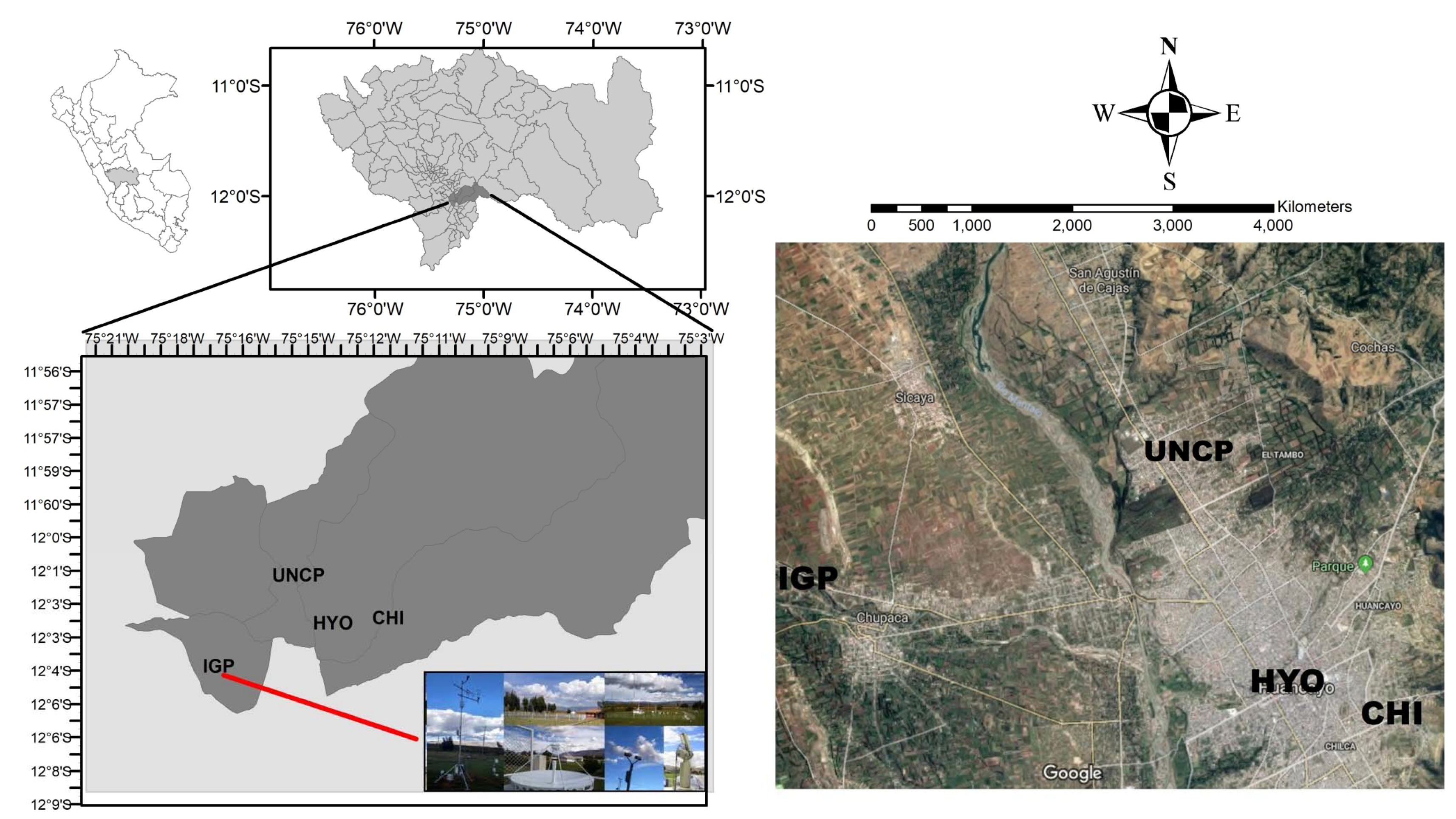
2.1. Area Description

The study was carried out in Huancayo city, the political capital of Junín region (Central Andes of Peru). This city is at about 3500 m above the sea level (m.a.s.l) and had an approximate population of 507,075 inhabitants [27]. Huancayo city is nestled in the Mantaro Valley that covers an area of 319.4 km2. It is bordered by mountains that act as natural barriers for air circulation and agricultural areas that produce significant amounts of different crops (i.e., vegetables, corn, potatoes) [28,29]. The automotive park counts with 64,576 vehicles [27] and probably is the main source of air pollution of the Metropolitan area. Pollutants may also be released from point sources, such as car repair, domestic heating systems, intensive agricultural practices, construction/demolition activities among others.
The climate at Huancayo city regularly is based on data collected at Observatory of Huancayo (IGP) from 1966 to 2002. Colder temperatures are recorded at June and July (winter) and the higher values are around October and December. The annual average temperature is 11.9 ± 1.2 °C. Precipitation has two marked seasons: dry and wet. From June to July the lowest rain amounts are recorded, meanwhile from January to March highest precipitation is recorded. February is the month with the highest record reaching an accumulated value of 129.1 mm. Mean annual accumulated precipitation is 752 ± 44.3 mm [30].

2.2. Sampling Method

24-h samples of PM2.5 were collected onto Teflon filter (47 mm PTFE, Whatman, NJ, USA) from March 2017 to November 2017 using Paired Partisol samplers (model 2000-FRM, Thermo Scientific, USA) set up to 2.5 µm inlet, flow rate of 16.7 L min−1 and about 24.0 m3 air samplers were used to collect samples in each monitoring station. A total of 151 samples (77 samples were used to analyze water-soluble ions and 74 for trace elements) of PM2.5 were collected at the four monitoring stations of Huancayo city (see Figure 1). Aerosol sampling was performed simultaneously at four monitoring stations collecting one sample by week and about five per month with 24 h sampling time. The locations of the monitoring stations relate the spatial distribution of three main districts that are considered Metropolitan Huancayo (Huancayo, El Tambo, and Chilca), where main commercial and transport activities are performed. The two first stations were installed in urban areas, very close to the downtown area, the third station (UNCP) was installed near the main highway, at 5.2 km to downtown. The last station (IGP) is located in a rural area, approximately 13.5 km of distance to Huancayo city. Table 1 presents a short description of monitoring stations. Blank filters also were considered for analysis. All filters collected were enclosed in Petri dishes (gamma radiation sterilized, VWR, USA), sealed with Teflon tape and placed within screwed aluminum holders, stored in coolers, and kept refrigerated at −20 °C until analysis.
The mass of the particles was calculated by the difference between the filter weight before and after sampling, and the concentration in the designated size range was computed by dividing the weight gain of the filter by the volume of the air sampled [31]. The filter weighing procedure was carried out in a temperature and humidity controlled clean room on a microbalance capable of making measurements of weight of objects of relatively small mass.

2.3. Extraction and Chemical Analysis

2.3.1. Water-Soluble Ion Content

Water soluble inorganic ions (anions and cations), were extracted in 10.0 mL of ultrapure water (18.2 MΩ cm) obtained from Milli-Q water (Milli-Q water purification system, Millipore Corp., Burlington, MA, USA), which was sonicated for 10 min. The extract was filtered through a 0.45 µm syringe filters of cellulose acetate membrane (Sartorius, Germany) [32]. Concentrations of water-soluble inorganic ions were measured by Ion Chromatography (Dionex ICS 5000 system, Thermo Fisher Scientific, Brazil) fitted with an ASRS-ULTRA self-regenerating suppressor and an Ion Pac AS4A-SC column by applying a Na2CO3/NaHCO3-eluent and additionally, a flow rate of 2 mL/min and sample injection volume was 25 µL were used, respectively. Single Standard solutions (Suprapure grade, Merck, Darmstadt, Germany) of anions and cations were used in different concentrations for a six-point external calibration. In total, seven ions: sulfate ( SO 4 2 ), nitrate ( NO 3 ), chloride (Cl), ammonium ( NH 4 + ), acetate (Ac) formate (Fo), and oxalate (Ox) were measured.

2.3.2. Trace Elements

For analysis of trace elements (Al, As, Ba, Ca, Cd, Cr, Cu, Fe, K, Mn, Ni, Pb, Rb, V, and Zn), filters were placed into a polytetrafluoroethylene (PTFE) flask, and then digested with 3 mL HNO3 (Suprapure grade, Merck, Darmstadt) at 120 °C for 4 h on a hot plate. After digestion, the samples were diluted to reach 5% HNO3, and the solution obtained was analyzed by inductively coupled plasma mass spectrometer (ICP–MS) Elan DRC II mass spectrometer (PerkinElmer SCIEX, Norwalk, CT, USA). Operating conditions for samples analysis by ICP–MS are presented in Table 2. 103Rh was used as internal standard (IS) to correct instrumental drifts and plasma fluctuations. Certified multi-element standards of trace elements were used to build a six-point external calibration was used to quantify the trace elements.

2.4. Quality Control

All samples were measured in triplicates and blank filters in both methods were also analyzed in parallel. To check the accuracy of digestion and analytical procedures, the standard reference material (SRM) of NIST 1648 “urban particulate matter” from the National Institute of Standards and Technology (NIST, Gaithersburg, USA) was analyzed. The limits of detection (LOD) and quantification (LOQ) were computed as three and ten times the standard deviation of ten blank measurements divided by the slope of the analytical curve. Table 3 shows the LOD, LOQ, and the extraction efficiencies of the SRM used. As can be seen, all results obtained were within the certified values, and extraction efficiencies ranged of 80–108% for all elements measured. Non-reported represents non-certified and non-measured elements from SRM 1648.

2.5. Methodology

2.5.1. Analysis of Variance and Tukey Test

One-way analysis of variance (ANOVA) was used to determine whether the mean daily ratios of the amounts of the examined pollutants differ significantly for each city. If ANOVA, based on F-test, detects a significant difference among these means, another test is then applied to determine that exactly which means differ significantly from the other [33]. There are several methods available for comparing means calculated from sub-samples of a sample [34]. A relatively simple but effective way is to use the Tukey test, In this work Least Significant Difference (LSD) Tukey test, which calculates the smallest significant between two means as if a test had been run on those two means [35]. This enables you make direct comparisons between two means from two individual groups.

2.5.2. Principal Component Analysis

Principal component analysis (PCA) is a dimension-reduction statistical technique that compresses the data by reducing the number of variables from a large set of variables to a small set of uncorrelated variables called principal components, without much loss of information [36]. The first component accounts for the largest possible variance (variability in the data), and each succeeding component accounts for as much of the remaining variability possible [37]. PCA with VARIMAX rotation was used, to identify potential sources emissions in the study area. The number of components was determined by Kaiser’s criterion—an eigenvalue >1 [38].

2.5.3. Hierarchical Cluster Analysis and Non-Hierarchical Cluster Analysis.

Actually, there are two main classes of clustering method: hierarchic and non-hierarchic methods. Hierarchical Cluster Analysis (HCA) generates a classification in which a small cluster of similar characteristics or properties are nested within larger clusters of less closely-related characteristics. Non-Hierarchical Cluster Analysis (NHCA) produces a classification by partitioning a dataset, giving a set of non-overlapping groups having no hierarchical relationships between them [39]. The optimal number of cluster usually determined through of K-means, and K-medoids algorithms. Both K-means and K-medoids attempt to minimize the distance between points labeled to be in a cluster and the point designated as the center of that cluster. K-means processes with the thought that new cluster should be formed according to the distance between points and center of clusters minimizing the Euclidean distances [40]. In contrast, K-Medoids or Partitioning Around Metoids (PAM) is a classical partitioning technique of clustering, which chooses data points as centers and can be used with arbitrary distances. The optimal number of cluster can be determined as follow: (1) compute clustering algorithm (k-means clustering) for different values of k; (2) for each k, calculate the total within-cluster sum of square (wss); (3) plot the curve of wss according to the number of clusters k; and (4) the location of a knee in the plot is generally considered as an indicator of the appropriate number of clusters [39]. When you use non-hierarchical cluster analysis, a logic way to determine the optimum number of clusters is as follows. The homogeneity within clusters can be measured by RMSD, defined as the sum of the root mean square deviations of cluster elements from the corresponding cluster center over clusters. The RMSD value usually decreases with an increasing number of clusters. Thus, this quantity itself is not very useful for deciding the optimal number of clusters. However, the change of RMSD (CRMSD) versus the change of cluster numbers, or even the change of CRMSD (CCRMSD) is much more informative. Therefore, working with cluster numbers from for example, 15 to 1, an optimal cluster number can be selected so as to maximize the change in CRMSD. The rationale behind this approach is that the number of clusters producing the largest improvement in cluster performance compared to that for a smaller number of clusters is considered optimal.
The grouping of data according to common properties is often based on the distance between the data. Some of these methods are: Euclidean distance and Mahalanobis distance [41]. The Euclidean distance treats each variable as equally important in calculating the distance, while Mahalanobis distance, which measures the distance between each observation in a multidimensional cloud of points and the centroid of the cloud [42]. The Euclidean distance between vectors x and y is represented in Equation (1), and the Mahalanobis distance D2 is showed in Equation (2).
d x , y 2 = ( x 1 y 1 ) 2 + ( x 2 y 2 ) 2
D 2 = ( x m ) V 1 ( x m )
where x is a vector of values for a particular observation, m is the vector of means of each variable, and V is the variance-covariance matrix. For high dimensional vectors, you might find that Manhattan works better than the Euclidean distance. The reason for this is quite simple to explain. Consider the case where we use the l norm that is the Minkowski distance with exponent = infinity. Then the distance is the highest difference between any two dimensions of your vectors. We can see that this does not make sense in many dimensions as we would be ignoring most of the dimensionality and measuring distance based on a single attribute. In this way, Mahalanobis metric takes into account different standard deviations of the components of the vectors as well as the correlations between the components [43]. In other words, using Mahalanobis metric, you can avoid that a major number of variables correlating with each other, namely involving less information compared to their number, are considered with unduly high weight when classifying, than a lower number of variables being non-correlated and, in this way, having the higher amount of information.
Hierarchical Cluster Analysis (HCA) using Ward’s method of linkage and the squared Euclidean distance for similarities was used to segregate associations within the group of trace elements and water-soluble ions to identify possible pollutant sources [40]. All statistical analyses were performed using CRAN R free software, version 3.3.2 [44] using the following R packages: factoextra [45], ggplot2 [46], cluster [47,48], and psych [49].

3. Results

3.1. Trace Element Contents and Water-Soluble Ion

Mean concentration ± standard deviation (S.D) and ANOVA results of fifteen trace elements: Al, As, Ba, Ca, Cd, Cr, Cu, Fe, K, Mn, Ni, Pb, Rb, V, and Zn and seven water-soluble ions: acetate (Ac), formate (Fo), chloride (Cl), nitrate ( NO 3 ), sulfate ( SO 4 2 ), ammonium ( NH 4 + ) and oxalate (Ox) from each monitoring station measured from PM2.5 are shown in Table 4. The highest concentrations of trace elements and water-soluble ions were observed in the two main urban areas (CHI and HYO). For instance, higher concentration levels of Al, As, Ca, Cd, Cr, Fe, Mn, Ni, Pb, Rb, V, Ac, Fo, Cl, and Ox were observed at CHI, while Ba, Cu, Zn, NO 3 , and NH 4 + were elevated at HYO where intense vehicular traffic is observed all day. Significant difference (p < 0.05) between mean of monitoring stations was observed for most elements, except for Ni, and V. No significant difference was found for most of the water-soluble ions, except for Fo, and Cl.
Altogether, the concentrations of most trace element and water-soluble ions at urban areas were higher than those at the rural area. The rural area is approximately 13.5 km away from the main urban area. Conversely, element concentrations of Al, As, Ca, Cd, Cu, Fe, Mn, P, Pb, Rb, Zn, and Cl from UNCP and rural area (IGP) were comparable.
The mass concentration of PM2.5 at UNCP, HYO, CHI, and IGP were 12.7 ± 4.47 µg/m3, 19.1 ± 6.26 µg/m3, 25.8 ± 11.0 µg/m3, and 8.8 ± 5.5 µg/m3, respectively (Figure 2). Higher PM2.5 mass concentrations were observed in the dry season (May to September) than wet season (March to April and October to November) (Figure 3). If ANOVA resulted in significant differences between the means of the pollutants, then the Tukey’s honestly significant difference test was applied in order to quantitatively compare the absolute values of the seasonal + site means of the examined pollutants (trace elements/water-soluble ions/PM2.5) between each season + site (pairwise multiple comparisons; Tukey 1985). From Figure 2 is observed a significant difference (p < 0.05) between main urban areas (CHI and HYO) and rural area (IGP) and urban area (UNCP) far downtown. In the Figure 3 is noted that only IGP area present significant difference between the dry and wet seasons.

3.2. Hierarchical Cluster Analysis

3.2.1. Trace Elements

Hierarchical cluster analysis (HCA) was applied to the concentration of trace elements and revealed two distinct groups. Group I was formed by Cd, As, Al, Ca, Mn, Rb, Cr, K, Fe, Ni, and Cu, the two last intimately linked, while Group II was formed by Ba, Zn, V, and Pb. A dendrogram depicting the Groups of trace elements is shown in Figure 4. The results indicate that elements belonging to the same group share similar characteristics and source of emission. The resulting dendrogram (Figure 4) suggest that group I may have a mixture of both natural and anthropogenic sources, while group II suggests elements released basically from anthropogenic activities.

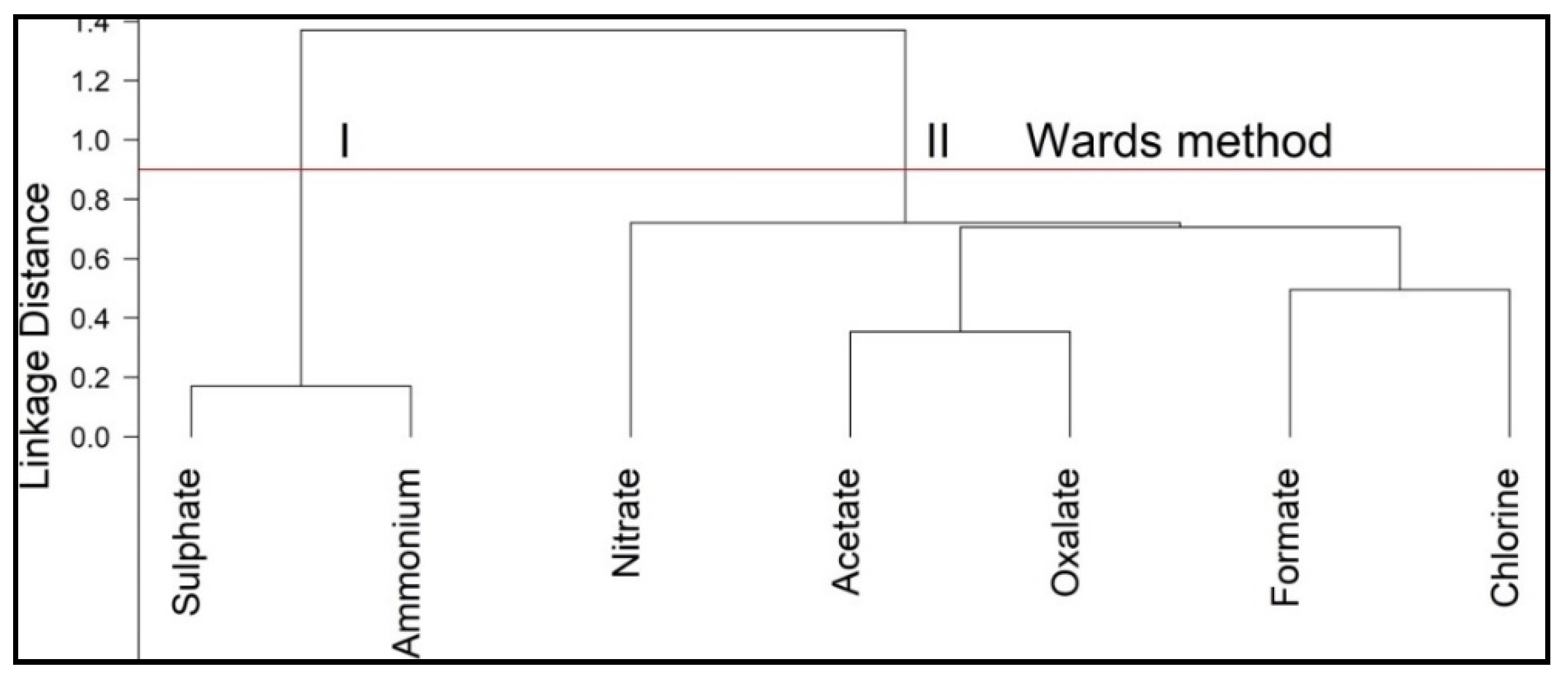
3.2.2. Water-Soluble Ions

The HCA applied to water-soluble ions concentrations (Figure 5) allowed dividing the ions into two main groups: sulfate ( SO 4 2 ) and ammonium ( NH 4 + ) constituting Group I. Group II was formed by nitrate ( NO 3 ), acetate (Ac), oxalate (Ox), formate (Fo), and chlorine (Cl). The groups formed suggest that the ions tested may have come from a common source [20]. Based on hierarchical clustering analysis (Figure 5), Group I indicates the grouping of secondary inorganic species. Group II shows NO 3 another secondary aerosol separated from others anions, while Ac and Ox linked intimately, and Fo and Cl also linked closely.

3.3. Principal Component Analysis

3.3.1. Trace Elements

The matrix with the concentration of fifteen elements from four monitoring stations (15 variables × 74 samples) was submitted to principal component analysis (PCA). The results of PCA after VARIMAX rotation are presented in Table 5. Two factors were obtained with Eigenvalues > 1, explaining 68% of the total variance in the data set. The Factor 1 accounts for 49% of the total variance and showed high positive loading for Al, As, Ca, Cd, Cr, Fe, K, Mn, and Rb (Table 5). Factor 2 explained 19% of the total variance and was observed high positive loadings among Ba, Pb, V, and Zn. Communalities of most elements were over 60% with the exception of Cd and Ni, whose commonalities are less than 60%.

3.3.2. Water-Soluble Ions

The matrix with the concentration of seven water-soluble ions from four monitoring stations (7 variables × 70 samples) was submitted to principal component analysis (PCA). The results of PCA after VARIMAX rotation are presented in Table 6. Two factors were obtained with Eigenvalues > 1, explaining 69% of the total variance in the data set. The Factor 1 accounts for 39% of the total variance and showed high positive loading for Ac, Fo, Cl, NO 3 , and Ox. Factor 2 explained 30% of the total variance and show high positive loadings between SO 4 2 and NH 4 + . Commonalities of all water-soluble ions were over 60%.

4. Discussion

Mean trace elements measured in PM2.5 samples decreased in the following order K > Fe > Ca > Al > Zn > Cr > Mn > Pb > Ba > Cu > Ni > V > As > Rb > Cd from macronutrients, micronutrients and trace elements. Likewise, water-soluble ions decreased in the following order: ammonium ( NH 4 + ) > nitrate ( NO 3 ) > formate (Fo), > chloride (Cl) > oxalate (Ox) > sulfate ( SO 4 2 ) > acetate (Ac). Highest PM2.5 mass concentration was observed in the monitoring stations of HYO (19.1 µg/m3) and CHI (25.8 µg/m3). These results are explained mainly because both monitored areas have more intense heavy traffic than UNCP (12.7 µg/m3) and IGP (8.8 µg/m3).
The PM2.5 mass concentration was found to range from 3.4 to 36.8 µg/m3 with an average value of 16.6 ± 6.8 µg/m3. This value is greater than prescribed by the National Ambient Air Quality Standards (NAAQS) (15.0 µg/m3), but minor than the Peruvian national Air Quality Standards (ECA) (25.0 µg/m3). This result is not surprising due to that Huancayo city is inside priority attention area, where urban areas have a population greater than 250,000, has a strong influence on commercial activities, and big vehicle fleet. Based on these results, therefore are needed the implement Air Quality Improvement Action Plans in Huancayo city. Higher PM2.5 mass concentrations were observed in the dry season (Figure 3) than wet season. As expected, wet removal/reduction of particulate matter by rainfall influence in the aerosol concentration of a pollutant atmosphere [50].
All element concentrations and water-soluble ions were evidently higher in the two main urban areas (HYO and CHI) inside the Metropolitan area of Huancayo. Both urban areas nested the main supermarkets, buildings, commerce and have a big vehicular fleet. For example, the highest concentration of Ba, Cu, and Zn were observed in HYO, while Pb, Ni, and V were elevated at CHI. According to Fijuwara et al. [51], Pb, Zn, and Ba are traffic markers, while Janta and Chantara [1], concluded that Cr, Pb, Cu, and Zn come mainly from vehicular sources. In addition, Querol et al. [52] suggested that Sb, Cu, Zn, Ba, and Fe are markers of brake or other vehicular parts wear and may be considered as indicators of re-suspension caused by traffic. Ba, V, Ni, Zn, Cu, and Sb, were also related to traffic emissions [53,54,55], while V and Ni were mostly associated with the oil combustion process from diesel engines [56,57]. According to the literature, we can conclude that Ba, Cu, Cr, Ni, Pb, Zn, and V may be correlated with vehicle emissions. It should be noted Peru has phased out leaded gasoline since 2009; however, Pb still presents into the environment of Metropolitan area of Huancayo may be due to past emissions and the fast increase in Huancayo’s vehicular fleet. For example, Pb is widely used in the manufacturing of different car components such as solder in electronics, lead-based paint, lead wheel weights, and lead-acid batteries, and their wear may release particles containing Pb [58].
Sulfate, nitrate and ammonium, three secondary inorganics comprise approximately 25–50% of the PM2.5 mass concentration [23,59] and are believed to originate from secondary transformation of their precursors such as SO2, NO2, and NH3 [60]. In Huancayo, NO 3 , and NH 4 + , dominated the water-soluble ions with elevated concentrations. Elevated nitrate was found in H and CHI, suggesting that this secondary aerosol might derive from vehicle emission, and ammonium concentration found at HYO may be ascribed to ammonia emission from a light-duty vehicle and IGP may be related to animal farming, fertilizers, and organic decomposition.
Sulfate aerosol is formed in the gas phase by reaction of sulfur dioxide (SO2) with OH to form SO3 which is then instantaneously converted into particulate sulfate. ( SO 4 2 ). SO 4 2 and Cl are typical tracers of coal combustion and major contribution in PM2.5 mass concentration [23].
The hierarchical cluster analyses (HCA) using either, trace elements (TE) or water-soluble ions (WSI) segregated two main groups. Based on previous reports, cluster of TE (Figure 4) containing Cd, K, Cr, As, Al, Fe, Ca, Mn, Rb, Ni, and Cu suggest a mixture of natural sources (Al, K, Mn, and Rb) and anthropogenic activities (Ca, Cd, Cr, Fe, and Ni), while Group 2 confirmed by Ba, Zn, V, and Pb suggests that anthropogenic activities such as vehicle sources for example, exhausts, re-suspension, and abrasion are the main pollution sources.
In relation to WSI (Figure 5), the cluster in Group 1 suggested that residential coal combustion and vehicle exhaust might be related to sulfate concentrations, while ammonium may be related to vehicular emissions from the light-duty vehicle. For instance, Dai et al. [61] showed direct evidence of sulfate emission from residential coal combustion present in particulate matter from Xian, China. Guo et al. [62] stated that one of the major sources of atmospheric sulfate is attributed to vehicle exhaust. Anthropogenic sulfate from fossil fuel combustion can be included in primary and secondary sulfate. Particulate ammonium mainly originates from ammonia vapor and ammonium salt particles [63] in form of ammonia are found in urban areas where gaseous ammonia reacts chemically with other compounds, leading to the formation of ‘‘smog”, which are respirable and can reach the alveoli, causing a number of respiratory disorders [64]. Elser et al. [65] presented high contributions of vehicular emissions to ammonia observed in three European urban cities: Zurich (Switzerland), Tartu (Estonia) and Tallin (Estonia). In Group 2, it clearly is observed that nitrate is separated of other elements, indicating that NO 3 may be released from vehicle emission.
PCA analysis of trace elements, in this study, segregated two groups. The first factor shows nine elements positively correlated with factor loadings higher than 0.60: Al, As, Ca, Cd, Cr, Fe, K, Mn, and Rb (Table 5). Elements, such as Al, K, Mn, and Rb are related to natural origin (geogenic sources), and As, Ca, Cd, Cr, and Fe are related to anthropogenic activities. Geogenic sources may be released by weathering of several minerals, especially silicates, carbonates, and oxides. Elevated calcium concentrations observed in H and CHI might be associated to release of this element during construction/demolition activities. Cadmium is a rare element (0.2 mg/kg in the earth crust), a non-nutritive element that may not likely be released by the soil. Cd can be added to the soil through natural (e.g., weathering of Cd-containing rocks, sea spray, volcanic activity) and anthropogenic activities (e.g., fossil fuel combustion, cadmium-nickel battery manufacture, fertilizer based on rock phosphate, and waste incineration) [7,66,67]. Therefore, we can conclude that the first groups may be ascribed to both natural sources (as result of soil re-suspended) and anthropogenic origin. In contrast, factor 2 showed elements of anthropogenic origin and suggest vehicular sources as the major sources.
PCA analysis of water-soluble ions segregated two groups. Five ions (acetate, formate, oxalate, chlorine, and nitrate) positively correlated with factor loading higher than 0.60 formed the factor 1. Factor 2 was represented by sulfate and ammonium positively correlated with factor loading higher than 0.60. Nitrate, sulfate, and ammonium showed higher values in urban areas from Huancayo Metropolitan, therefore, we may suppose that vehicular emission and posterior chemical transformation as the main pollutant source of these ions.
PCA and HCA multivariate statistical techniques indicate that there are two main sources of trace elements and water-soluble ions contained in PM2.5 collected from four monitoring stations inside the Metropolitan area of Huancayo. Both multivariate techniques suggested that Ba, Pb, V, and Zn are release from anthropogenic origin. Likewise, nitrate, sulfate, and ammonium are probably formed from vehicle emission precursors such as SO2, NO2, and NH3.
The results obtained in this study confirm that urban activities and heavy vehicular flux (big fleet vehicular) can be emission sources of trace elements and water-soluble ions into the Metropolitan Huancayo.

5. Conclusions

The present study is probably the first report on trace element levels and water-soluble ions from PM2.5 collected at four monitoring stations of Metropolitan Huancayo (Peru). The PM2.5 results offer a preliminary assessment and a general idea of the state of air quality from the study area. The highest annual PM2.5 concentrations were found at monitoring stations of CHI (25.8 µg/m3) and HYO (19.1 µg/m3). In contrast, the lowest annual concentration for PM2.5 was observed at monitoring stations of UNCP (12.7 µg/m3) and IGP (8.8 µg/m3). On the other hand, the monitoring of the station of HYO and CHI has exceeded the Peruvian national air quality standards and WHO thresholds.
PM2.5 samples collected in the main urban areas (HYO and CHI) show higher concentrations of trace elements and water-soluble ions than those of rural area. HCA and PCA results showed consistent segregation of trace elements and water-soluble ions. Most trace elements (Al, As, Cd, Ca, Mn, Rb, Cr, K, Fe, Ni, and Cu) were related to a combination of both anthropogenic and natural origin (soil re-suspension), while Ba, Zn, V, and Pb were related to vehicle sources. The water-soluble ions may be derived from vehicular emissions. Therefore, the present work confirms that the main contaminations are related to soil dust and vehicular sources.

Author Contributions

A.H.D.L.C.: data processing and handling; manuscript writing; production of figures. Y.B.R.: conceptualization; project administration; funding acquisition. L.S.-S.: initial idea for study; funding acquisition; data collection, and writing and reviewing the manuscript. J.P: methodology; funding acquisition. D.A.T.: data collection. A.G.: chemical data contribution.

Funding

This research was funded by InnóvatePerú-trough contract 324-PNICP-PIAP-2015 granted to Universidad Nacional del Centro del Perú.

Acknowledgments

Thanks to Coordenação de Aperfeiçoamento de Pessoal de Nível Superior (CAPES, Brazil) and Conselho Nacional de Desenvolvimento Científico e Tecnológico (CNPq, Brazil). Also we would like to thanks to Fondo Italo Peruano (FIP) and the NGO Protection Ambiental y Desarrollo Sostenible (PADES) leading member of the Environmental Dialogue Round Table of Junin Region (MEDIAREJ) for providing their aerosol samplers.We appreciate three anonymous reviewers, which improved the manuscript.

Conflicts of Interest

The authors declare no conflict of interest.

References

  1. Janta, R.; Chantara, S. Tree bark as bioindicator of metal accumulation from road traffic and air quality map: A case study of Chiang Mai, Thailand. Atmos. Pollut. Res. 2017, 8, 956–967. [Google Scholar] [CrossRef]
  2. Morais, S.; Garcia, F.; de Pereira, M.L. Heavy Metals and Human Health. In Environmental Health—Emerging Issues and Practice; IntechOpen: London, UK, 2012; Volume 10, pp. 227–246. ISBN 9789537619343. [Google Scholar]
  3. Mateus, V.L.; Monteiro, I.L.G.; Rocha, R.C.C.; Saint’Pierre, T.D.; Gioda, A. Study of the chemical composition of particulate matter from the Rio de Janeiro metropolitan region, Brazil, by inductively coupled plasma-mass spectrometry and optical emission spectrometry. Spectrochim. Acta Part B At. Spectrosc. 2013, 86, 131–136. [Google Scholar] [CrossRef]
  4. EPA Particulate Matter (PM) Pollution. Available online: https://www.epa.gov/pm-pollution/particulate-matter-pm-basics (accessed on 29 December 2018).
  5. Polichetti, G.; Cocco, S.; Spinali, A.; Trimarco, V.; Nunziata, A. Effects of particulate matter (PM10, PM2.5 and PM1) on the cardiovascular system. Toxicology 2009, 261, 1–8. [Google Scholar] [CrossRef] [PubMed]
  6. Chirino, Y.I.; Sánchez-pérez, Y.; Osornio-vargas, Á.R.; Rosas, I.; García-cuellar, C.M. Sampling and composition of airborne particulate matter (PM 10) from two locations of Mexico City. Data Brief 2015, 4, 353–356. [Google Scholar] [CrossRef] [PubMed]
  7. WHO. Air Quality Guidelines for Europe, 2nd ed.; WHO: Copenhagen, Denmark, 2000; ISBN 9289013583. [Google Scholar]
  8. Wu, W.; Jin, Y.; Carlsten, C. Clinical reviews in allergy and immunology Inflammatory health effects of indoor and outdoor particulate matter. J. Allergy Clin. Immunol. 2019, 141, 833–844. [Google Scholar] [CrossRef] [PubMed]
  9. Song, Y.; Wang, X.; Maher, B.A.; Li, F.; Xu, C. The spatial-temporal characteristics and health impacts of ambient fi ne particulate matter in China. J. Clean. Prod. 2016, 112, 1312–1318. [Google Scholar] [CrossRef]
  10. Kim, K.-H.; Kabir, E.; Kabir, S. A review on the human health impact of airborne particulate matter. Environ. Int. 2015, 74, 136–143. [Google Scholar] [CrossRef] [PubMed]
  11. Pulong, C.; Tijian, W.; Mei, D.; Kasoar, M.; Yong, H.; Min, X.; Shu, L.; Bingliang, Z. Characterization of major natural and anthropogenic source pro fi les for size-fractionated PM in Yangtze River Delta. Sci. Total Environ. 2017, 598, 135–145. [Google Scholar] [CrossRef]
  12. Steinnes, E.; Lierhagen, S. Geographical distribution of trace elements in natural surface soils: Atmospheric in fl uence from natural and anthropogenic sources. Appl. Geochem. 2018, 88, 2–9. [Google Scholar] [CrossRef]
  13. Bharti, P.K. Heavy Metals in Environment; Lambert Academic Publishing: Saarbrucken, Germany, 2012; ISBN 9783659151330. [Google Scholar]
  14. Clements, N.; Eav, J.; Xie, M.; Hannigan, M.P.; Miller, S.L.; Navidi, W.; Peel, J.L.; Schauer, J.J.; Shafer, M.M.; Milford, J.B. Concentrations and source insights for trace elements in fine and coarse particulate matter. Atmos. Environ. 2014, 89, 373–381. [Google Scholar] [CrossRef]
  15. Ventura, L.M.B.; Mateus, V.L.; Collett, A.; Leitão, S.; Wanderley, K.B.; Taira, F.T.; Pierre, T.D.; Saint Gioda, A. Chemical composition of fine particles (PM2.5 ): Water-soluble organic fraction and trace metals. Air Qual. Atmos. Health 2017, 845–852. [Google Scholar] [CrossRef]
  16. Vianna, N.A.; Gonçalves, D.; Brandão, F.; de Barros, R.P.; Filho, G.M.A.; Meire, R.O.; Torres, J.P.M.; Malm, O.; Júnior, A.D.O.; Andrade, L.R. Assessment of heavy metals in the particulate matter of two Brazilian metropolitan areas by using Tillandsia usneoides as atmospheric biomonitor. Environ. Sci. Pollut. Res. 2011, 18, 416–427. [Google Scholar] [CrossRef] [PubMed]
  17. Srinivasa Gowd, S.; Ramakrishna Reddy, M.; Govil, P.K. Assessment of heavy metal contamination in soils at Jajmau (Kanpur) and Unnao industrial areas of the Ganga Plain, Uttar Pradesh, India. J. Hazard. Mater. 2010, 174, 113–121. [Google Scholar] [CrossRef] [PubMed]
  18. Wang, H.; Qiao, B.; Zhang, L.; Yang, F.; Jiang, X. Characteristics and sources of trace elements in PM2.5 in two megacities in Sichuan Basin of southwest China. Environ. Pollut. 2018, 242, 1577–1586. [Google Scholar] [CrossRef]
  19. De La Cruz, A.R.H.; De La Cruz, J.K.H.; Tolentino, D.A.; Gioda, A. Trace element biomonitoring in the Peruvian andes metropolitan region using Flavoparmelia caperata lichen. Chemosphere 2018, 210, 849–858. [Google Scholar] [CrossRef]
  20. Zhou, H.; Lü, C.; He, J.; Gao, M.; Zhao, B.; Ren, L.; Zhang, L.; Fan, Q.; Liu, T.; He, Z.; et al. Stoichiometry of water-soluble ions in PM2.5: Application in source apportionment for a typical industrial city in semi-arid region, Northwest China. Atmos. Res. 2018, 204, 149–160. [Google Scholar] [CrossRef]
  21. Rao, P.S.P.; Tiwari, S.; Matwale, J.L.; Pervez, S.; Tunved, P.; Safai, P.D.; Srivastava, A.K.; Bisht, D.S.; Singh, S.; Hopke, P.K. Sources of chemical species in rainwater during monsoon and non-monsoonal periods over two mega cities in India and dominant source region of secondary aerosols. Atmos. Environ. 2016, 146, 90–99. [Google Scholar] [CrossRef] [Green Version]
  22. Phillips-smith, C.; Jeong, C.; Healy, R.M.; Dabek-zlotorzynska, E.; Celo, V. Sources of particulate matter components in the Athabasca oil sands region: Investigation through a comparison of trace element measurement methodologies. Atmos. Chem. Phys. 2017, 9435–9449. [Google Scholar] [CrossRef]
  23. Sun, Z.; Duan, F.; He, K.; Du, J.; Zhu, L. Sulfate–nitrate–ammonium as double salts in PM2.5: Direct observations and implications for haze events. Sci. Total Environ. 2019, 647, 204–209. [Google Scholar] [CrossRef]
  24. Soleimani, M.; Amini, N.; Sadeghian, B.; Wang, D.; Fang, L. Heavy metals and their source identification in particulate matter (PM2.5) in Isfahan City, Iran. J. Environ. Sci. (China) 2018, 72. [Google Scholar] [CrossRef]
  25. Silva, J.; Rojas, J.; Norabuena, M.; Molina, C.; Toro, R.A.; Leiva-Guzmán, M.A. Particulate matter levels in a South American megacity: The metropolitan area of Lima-Callao, Peru. Environ. Monit. Assess. 2017, 189. [Google Scholar] [CrossRef] [PubMed]
  26. Suarez-Salas, L.; Alvarez Tolentino, D.; Bendezú, Y.; Pomalaya, J. Caracterización química del material particulado atmosférico del centro urbano de Huancayo, Perú. Rev. Soc. Quím Perú 2017, 83, 187–199. [Google Scholar]
  27. Instituto Nacional de Estadística e Informática. Peru: Principales Indicadores Departamentales 2009–2016; Instituto Nacional de Estadística e Informática: Lima, Peru, 2017.
  28. Serrano, F. Environmental Contamination in the Homes of La Oroya and Concepcion and Its Effects in the Health of Community Residents. 2002. Available online: https://lib.ohchr.org/HRBodies/UPR/Documents/Session2/PE/EJ-AIDA_PER_UPR_S2_2008anx_StudyofcontaminationinLaOroya.pdf (accessed on 4 December 2018).
  29. Milan, A.; Ho, R. Livelihood and migration patterns at different altitudes in the Central Highlands of Peru. Clim. Dev. 2014, 6, 69–76. [Google Scholar] [CrossRef]
  30. IGP. Atlas Climático de Precipitacion y Temperatura del aire en la Cuenca del Rio Mantaro, 1st ed.; Del Ambiente, C.-C.N., Ed.; Depósito legal en la Biblioteca Nacional del Perú: San Borja, Peru, 2005; ISBN 9972824136.
  31. Pfeiffer, R.L. Sampling For PM10 and PM2.5 Particulates. Publ. USDA-ARS 2005, 1, 20. [Google Scholar]
  32. Villalobos, A.M.; Barraza, F.; Jorquera, H.; Schauer, J.J. Chemical speciation and source apportionment of fine particulate matter in Santiago, Chile, 2013. Sci. Total Environ. 2015, 512–513, 133–142. [Google Scholar] [CrossRef] [PubMed]
  33. Sawyer, S.F. Analysis of Variance: The Fundamental Concepts. J. Man. Manip. Ther. 2007, 17, 27–38. [Google Scholar] [CrossRef]
  34. Hilton, A.C.; Armstrong, R. Stat Note 6:post-hoc ANOVA tests. Microbiologist 2006, 6, 4. [Google Scholar]
  35. Lynne, W.J.; Abdi, H. Fisher’s Least Significant Difference (LSD) Test. Encycl. Res. Des. 2010, 1–6. [Google Scholar] [CrossRef]
  36. James, G.; Witten, D.; Hastie, T.; Tibshirani, R. An Introduction to Statistical Learning with Applications in R; Olkin, G.C.S.F.I., Ed.; Springer: New York, NY, USA, 2015; Volume 6, ISBN 9781461471370. [Google Scholar]
  37. Jolliffe, I.T.; Cadima, J.; Cadima, J. Principal component analysis: A review and recent developments. Philos. Trans. R. Soc. A-Math. Phys. Eng. Sci. 2016. [Google Scholar] [CrossRef]
  38. Kaiser, H.F. The application of electronic computers to factor analysis. Educ. Psychol. Meas. 1960, 20, 141–151. [Google Scholar] [CrossRef]
  39. Gülağız, F.K.; Şahin, S. Comparison of Hierarchical and Non-Hierarchical Clustering Algorithms. Int. J. Comput. Eng. Inf. Technol. 2017, 9, 6–14. [Google Scholar]
  40. Hastie, T.; Tibshirani, R.; Friedman, J. The Elements of Statistical Learning: Data Mining, Inference and Prediction, 2nd ed.; Springer Series in Statistics; Springer: New York, NY, USA, 2009; Volume 27, ISBN 978-0-387-84857-0. [Google Scholar]
  41. Kumar, N.; Bansal, A.; Sarma, G.S.; Rawal, R.K. Chemometrics tools used in analytical chemistry: An overview. Talanta 2014, 123, 186–199. [Google Scholar] [CrossRef] [PubMed]
  42. Baaijens, J.A.; Draisma, J. Euclidean distance degrees of real algebraic groups. Linear Algebra Its Appl. 2015, 467, 174–187. [Google Scholar] [CrossRef] [Green Version]
  43. Melnykov, I.; Melnykov, V. On K-means algorithm with the use of Mahalanobis distances. Stat. Probab. Lett. 2014, 84, 88–95. [Google Scholar] [CrossRef]
  44. R Team Core. A language and Environment for Statistical Computing. In R Foundation for Statistical Computing, Vienna Austria; R Foundation for Statistical Computing: Vienna, Austria, 2015. [Google Scholar]
  45. Kassambara, A.; Mundt, F. Extract and Visualize the Results of Multivariate Data Analyses. R Packag. Version 2016, 1. Available online: https://rpkgs.datanovia.com/factoextra/index.html (accessed on 4 December 2018).
  46. Wickham, M.H.; Chang, W. An Implementation of the Grammar of Graphics; Springer: New York, NY, USA, 2016; ISBN 978-3-319-24277-4. [Google Scholar]
  47. Chavent, M.; Simonet, V.K.; Liquet, B.; Kuentz-simonet, V. ClustOfVar: An R Package for the Clustering of Variables. J. Stat. 2012, 50, 1–16. [Google Scholar]
  48. Maechler, M.; Rousseeuw, P.; Struyf, A.; Hubert, M.; Hornik, K.; Studer, M.; Roudier, P. Finding Groups in Data: Cluster Analysis Extended Rousseeuw. 2015. Available online: https://stat.ethz.ch/R-manual/R-devel/library/cluster/html/00Index.html (accessed on 4 December 2018).
  49. Revelle, W. Procedures for Psychological, Psychometric, and Personality Research 2018, 443. Available online: https://cran.r-project.org/web/packages/psych/index.html (accessed on 4 December 2018).
  50. Xu, D.; Ge, B.; Wang, Z.; Sun, Y.; Chen, Y.; Ji, D.; Yang, T.; Ma, Z.; Cheng, N.; Hao, J.; et al. Below-cloud wet scavenging of soluble inorganic ions by rain in Beijing during the summer of 2014. Environ. Pollut. 2017, 230, 963–973. [Google Scholar] [CrossRef] [PubMed]
  51. Fujiwara, F.G.; Gómez, D.R.; Dawidowski, L.; Perelman, P.; Faggi, A. Metals associated with airborne particulate matter in road dust and tree bark collected in a megacity (Buenos Aires, Argentina). Ecol. Indic. 2011, 11, 240–247. [Google Scholar] [CrossRef]
  52. Querol, X.; Alastuey, A.; Moreno, T.; Viana, M.M.; Castillo, S.; Pey, J.; Rodríguez, S.; Artiñano, B.; Salvador, P.; Sánchez, M.; et al. Spatial and temporal variations in airborne particulate matter (PM10 and PM2.5) across Spain 1999–2005. Atmos. Environ. 2008, 42, 3964–3979. [Google Scholar] [CrossRef]
  53. Godoy, M.L.D.P.; Godoy, J.M.; Roldão, L.A.; Soluri, D.S.; Donagemma, R.A. Coarse and fine aerosol source apportionment in Rio de Janeiro, Brazil. Atmos. Environ. 2009, 43, 2366–2374. [Google Scholar] [CrossRef]
  54. Guéguen, F.; Stille, P.; Dietze, V.; Gieré, R. Chemical and isotopic properties and origin of coarse airborne particles collected by passive samplers in industrial, urban, and rural environments. Atmos. Environ. 2012, 62, 631–645. [Google Scholar] [CrossRef]
  55. Enamorado-Báez, S.M.; Gómez-Guzmán, J.M.; Chamizo, E.; Abril, J.M. Levels of 25 trace elements in high-volume air filter samples from Seville (2001–2002): Sources, enrichment factors and temporal variations. Atmos. Res. 2015, 155, 118–129. [Google Scholar] [CrossRef] [Green Version]
  56. Rizzio, E.; Bergamaschi, L.; Valcuvia, M.; Profumo, A.; Gallorini, M. Trace elements determination in lichens and in the airborne particulate matter for the evaluation of the atmospheric pollution in a region of northern Italy. Environ. Int. 2001, 26, 543–549. [Google Scholar] [CrossRef]
  57. Giampaoli, P.; Wannaz, E.D.; Tavares, A.R.; Domingos, M. Suitability of Tillandsia usneoides and Aechmea fasciata for biomonitoring toxic elements under tropical seasonal climate. Chemosphere 2016, 149, 14–23. [Google Scholar] [CrossRef] [PubMed]
  58. Song, S.; Wu, Y.; Jiang, J.; Yang, L.; Cheng, Y.; Hao, J. Chemical characteristics of size-resolved PM2.5 at a roadside environment in Beijing, China. Environ. Pollut. 2012, 161, 215–221. [Google Scholar] [CrossRef] [PubMed]
  59. Li, X.; Wang, L.; Wang, Y.; Wen, T.; Yang, Y.; Zhao, Y.; Wang, Y. Chemical composition and size distribution of airborne particulate matters in Beijing during the 2008 Olympics. Atmos. Environ. 2012, 50, 278–286. [Google Scholar] [CrossRef]
  60. Wang, Y.; Zhuang, G.; Zhang, X.; Huang, K.; Xu, C.; Tang, A.; Chen, J.; An, Z. The ion chemistry, seasonal cycle, and sources of PM2.5and TSP aerosol in Shanghai. Atmos. Environ. 2006, 40, 2935–2952. [Google Scholar] [CrossRef]
  61. Dai, Q.; Bi, X.; Song, W.; Li, T.; Liu, B.; Ding, J.; Xu, J.; Song, C.; Yang, N.; Schulze, B.C.; et al. Residential coal combustion as a source of primary sulfate in Xi’an, China. Atmos. Environ. 2019, 196, 66–76. [Google Scholar] [CrossRef]
  62. Guo, Z.; Shi, L.; Chen, S.; Jiang, W.; Wei, Y.; Rui, M.; Zeng, G. Sulfur isotopic fractionation and source appointment of PM2.5in Nanjing region around the second session of the Youth Olympic Games. Atmos. Res. 2016, 174–175, 9–17. [Google Scholar] [CrossRef]
  63. Ho, K.F.; Lee, S.C.; Chan, C.K.; Yu, J.C.; Chow, J.C.; Yao, X.H. Characterization of chemical species in PM2.5 andPM10 aerosols in Hong Kong. Atmos. Environ. 2003, 37, 31–39. [Google Scholar] [CrossRef]
  64. Kim, Y.; Lee, I.; Lim, C.; Farquhar, J.; Lee, S.M.; Kim, H. The origin and migration of the dissolved sulfate from precipitation in Seoul, Korea. Environ. Pollut. 2018, 237, 878–886. [Google Scholar] [CrossRef]
  65. Elser, M.; El-Haddad, I.; Maasikmets, M.; Bozzetti, C.; Wolf, R.; Ciarelli, G. High contributions of vehicular emissions to ammonia in three European cities derived from mobile measurements. Atmos. Environ. 2018, 175, 210–220. [Google Scholar] [CrossRef]
  66. Roberts, T.L. Cadmium and Phosphorous Fertilizers: The Issues and the Science. Procedia Eng. 2014, 83, 52–59. [Google Scholar] [CrossRef] [Green Version]
  67. Hazotte, C.; Leclerc, N.; Meux, E.; Lapicque, F. Direct recovery of cadmium and nickel from Ni-Cd spent batteries by electroassisted leaching and electrodeposition in a single-cell process. Hydrometallurgy 2016, 162, 94–103. [Google Scholar] [CrossRef]
Figure 1. Location of the monitoring stations. The map was prepared with Arc GIS 10.0 software.
Atmosphere 10 00021 g001
Figure 2. Boxplot of mean mass concentration ± standard deviation (S.D.) of PM2.5 at each monitoring station. Means with the same letter and color (a and b) code are not significantly different (Tukey multiple comparisons of means, p < 0.05). Red line = 25 µg m−3 value of National Air Quality Standards (ECA in Spanish) from Peru.
Atmosphere 10 00021 g002
Figure 3. Boxplot mean mass concentration ± standard deviation (S.D.) of PM2.5 at each monitoring station for the dry season (May to September) and the wet season (March, April, October, and November). Means with the same letter (a and b) code are not significantly different (Tukey multiple comparisons of means, p < 0.05).
Atmosphere 10 00021 g003
Figure 4. Results of the hierarchical cluster analysis (dendrogram) of the trace element concentrations measured in PM2.5.
Atmosphere 10 00021 g004
Figure 5. Results of the hierarchical cluster analysis (dendrogram) of the water-soluble ions concentrations measured in PM2.5.
Atmosphere 10 00021 g005
Table 1. Short description of the monitoring stations.
Monitoring StationLatitude
Longitude
Population of the District ADescription
Huancayo (HYO)12° 4′ 12.03″ S
75° 12′ 43.55″ W
117,559Downtown, is a residential and commercial area with heavy traffic from automobiles, trucks, bus, railway, and motorbike.
Chilca (CHI)12° 4′ 21.51″ S
75° 11′ 32.46″ W
86,496Located aside downtown, is a residential, commercial and nestled small industries. The traffic is intense all days
El Tambo (UNCP)12° 1′ 57.28″ S
75° 14′ 8.38″ W
160.685Located 5.2 km far from downtown and has a medium traffic flow. The equipment was installed at the roof of the administrative building of the National University of the Center of Peru
Observatory Huancayo (IGP)12° 2′ 59.28″ S
75° 20′ 24.58″ W
5929Located 13.5 km far from downtown, is a rural area, dominated by agriculture fields where the Geophysical Institute of Peru has its installations.
A Estimated population 2016 [27].
Table 2. Operating conditions for the inductively coupled plasma mass spectrometry (ICP–MS) measurements.
ICP-MS OperationValue
RF power (W)1150
Frequency (MHz)27.2
Plasma gas flow rate (L min−1)11.5
Auxiliary gas flow rate (L min−1)0.55
Nebulizer gas flow rate (L min−1)0.98
Sample uptake rate (mL min−1)0.6
Measurement modeDual (PC/analog)
Acquisition time (s)1
Dwell time (ms)200
Replicates6
Table 3. Limits of detection (LOD) and limits of quantification (LOQ) by ICP–MS and concentration of Certified Reference Material of urban particulate matter NIST SRM 1648 used to evaluate the extraction efficiencies.
ElementsLOD (µg g−1)LOQ (µg g−1)CRM—Urban Particulate Matter
Certified Value (µg g−1)Found Value (µg g−1)% Extracted
Al0.200.6534,300 ± 130028,000 ± 210081.5
As0.0060.020115.5 ± 3.9108 ± 4.2108
Ba0.0100.032---
Ca0.832.7458,400 ± 190058,800101
Cd0.0010.00273.7 ± 2.379.3 ± 3.1108
Cr0.0230.077402 ± 13320 ± 2080
Cu0.0170.057610 ± 70657 ± 31108
Fe0.270.8739,200 ± 210042,000 ± 2200107
K0.331.0810,560 ± 4908790 ± 34083.2
Mn0.0140.046790 ± 44823 ± 34104
Ni0.0080.02881.1 ± 6.886.2 ± 4.2106
Pb0.0040.0136550 ± 337063 ± 21108
Rb0.0020.00651.0 ± 1.542.2 ± 2.1283
V0.0020.007127 ± 11136 ± 8107
Zn0.0410.1364800 ± 2704710 ± 16798
- Non-reported.
Table 4. Comparison of mean concentration values (± standard deviation, SD) in µg m−3 and results of the analysis of variance (ANOVA) of the trace elements and water-soluble ions measured in PM2.5 collected at each monitoring station from the Metropolitan area of Huancayo city, Junín, Peru.
ElementIGPUNCPHYOCHIANOVA
N = 16N = 20N = 16N = 22p-Value A
Al0.651 ± 0.563 b0.874 ± 0.785 b1.440 ± 1.222 b2.719 ± 1.868 a***
As0.002 ± 0.002 c0.006 ± 0.003 c0.010 ± 0.005 b0.014 ± 0.007 a***
Ba0.008 ± 0.006 b0.027 ± 0.033 c0.100 ± 0.188 a0.087 ± 0.082 a*
Ca0.807 ± 0.968 b1.326 ± 0.781 b4.160 ± 2.684 a6.413 ± 4.506 a***
Cd0.001 ± 0.001 b0.002 ± 0.002 b0.003 ± 0.003 b0.008 ± 0.007 a***
Cr0.045 ± 0.030 a0.088 ± 0.034 c0.132 ± 0.055 b0.196 ± 0.074 d***
Cu0.012 ± 0.012 b0.020 ± 0.019 b0.077 ± 0.126 a0.075 ± 0.054 a**
Fe0.932 ± 0.805 c1.348 ± 0.752 c2.817 ± 1.938 b5.064 ± 3.139 a***
K1.826 ± 1.987 c3.166 ± 2.059 b2.889 ± 1.112 b8.104 ± 3.499 a***
Mn0.016 ± 0.013 c0.037 ± 0.024 c0.094 ± 0.073 a0.182 ± 0.128 b***
Ni0.004 ± 0.0030.004 ± 0.0050.008 ± 0.0050.022 ± 0.0500.19
Pb0.005 ± 0.005 b0.024 ± 0.026 b0.060 ± 0.078 b0.153 ± 0.144 a***
Rb0.001 ± 0.001 c0.002 ± 0.002 c0.004 ± 0.004 b0.009 ± 0.006 a***
V0.004 ± 0.0030.001 ± 0.0010.005 ± 0.0080.015 ± 0.0420.32
Zn0.145 ± 0.277 b0.146 ± 0.093 b0.719 ± 1.221 a0.461 ± 0.275 a*
IonsIGPUNCPHYOCHIANOVA
N = 18N = 18N = 20N = 21p-Value A
Ac0.001 ± 0.0010.001 ± 0.0010.001 ± 0.0010.002 ± 0.0010.08
Fo0.011 ± 0.008 b0.004 ± 0.004 c0.008 ± 0.007 c0.023 ± 0.011 a***
Cl0.005 ± 0.005 c0.006 ± 0.005 c0.012 ± 0.009 b0.018 ± 0.012 a***
NO 3 0.034 ± 0.0500.023 ± 0.0140.059 ± 0.0840.055 ± 0.0270.16
SO 4 2 0.006 ± 0.0060.005 ± 0.0060.007 ± 0.0070.007 ± 0.0050.67
NH 4 + 0.240 ± 0.3500.219 ± 0.3590.303 ± 0.4490.191 ± 0.2880.83
Ox0.010 ± 0.0100.008 ± 0.0050.009 ± 0.0050.010 ± 0.0050.78
A Values on each horizontal line followed by the same letter do not differ significantly (p = 0.05). * Significant at 0.05 probability level. ** Significant at 0.01 probability level. *** Significant at 0.001 probability level. N = number of individual samples collected in each monitoring station.
Table 5. Factor (Fa) loadings of the two extracted factors (principal component analysis, varimax standardized rotation) for PM2.5 samples (element concentration of 24-h samples in µg/m3), together with the respective communalities (comm). Loadings superior to 0.60 (in bold) are considered as significant.
ElementFactors
Fa1Fa2Comm
PM2.5
Al0.920.110.85
As0.900.220.87
Ba0.360.620.71
Ca0.930.180.91
Cd0.690.110.57
Cr0.680.590.63
Cu0.450.280.72
Fe0.900.130.88
K0.840.200.76
Mn0.950.210.95
Ni0.290.090.51
Pb0.280.850.80
Rb0.930.240.93
V−0.100.820.82
Zn0.170.650.67
Eigenvalue7.302.83
% of total variance0.490.19
% of cumulative variance0.490.68
Principal component analysis (PCA) with Varimax rotation, Kaiser–Meyer–Olkin (KMO) measure of sampling adequacy.
Table 6. Factor (Fa) loadings of the two extracted factors (principal component analysis, Varimax standardized rotation) for PM2.5 samples (water-soluble ions concentration of 24-h samples in µg/m3), together with the respective communalities (comm). Loadings superior to 0.60 (in bold) are considered as significant.
ElementFactors
Fa1Fa2Comm
PM2.5
Ac0.660.390.62
Fo0.640.000.61
Cl0.800.110.71
N O 3 0.840.300.79
S O 4 2 0.230.870.80
Ox0.690.430.66
Eigenvalue2.732.08
% of total variance0.390.30
% of cumulative variance0.390.69
Principal component analysis (PCA) with Varimax rotation, Kaiser–Meyer–Olkin (KMO) measure of sampling adequacy.

