Analysis of Possible Triggering Mechanisms of Severe Thunderstorms in the Tropical Central Andes of Peru, Mantaro Valley

 ,
,  ,
, 
Abstract
:1. Introduction
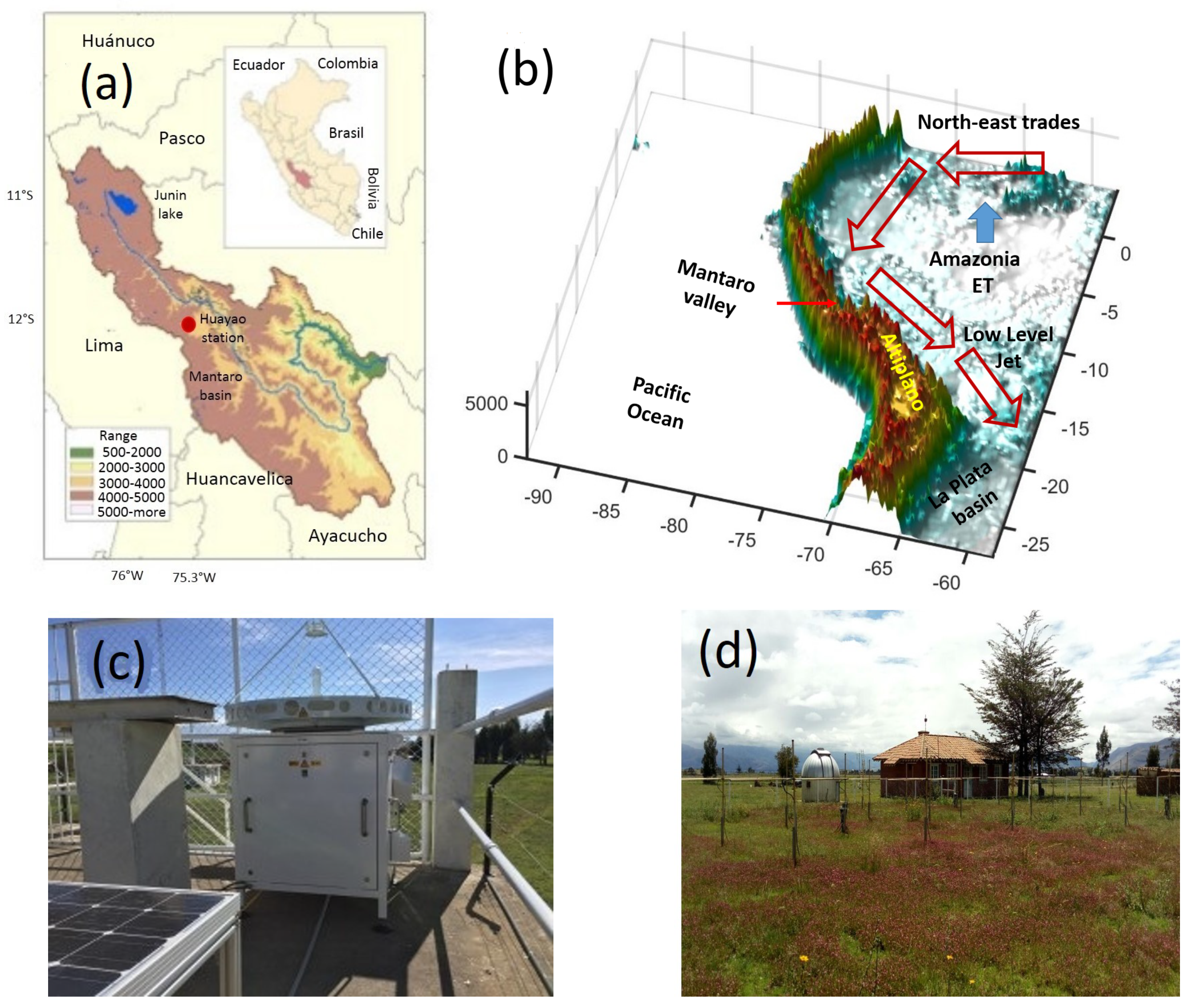
2. Site and Location
3. Methodology and Data
3.1. The Water Vapor Flux
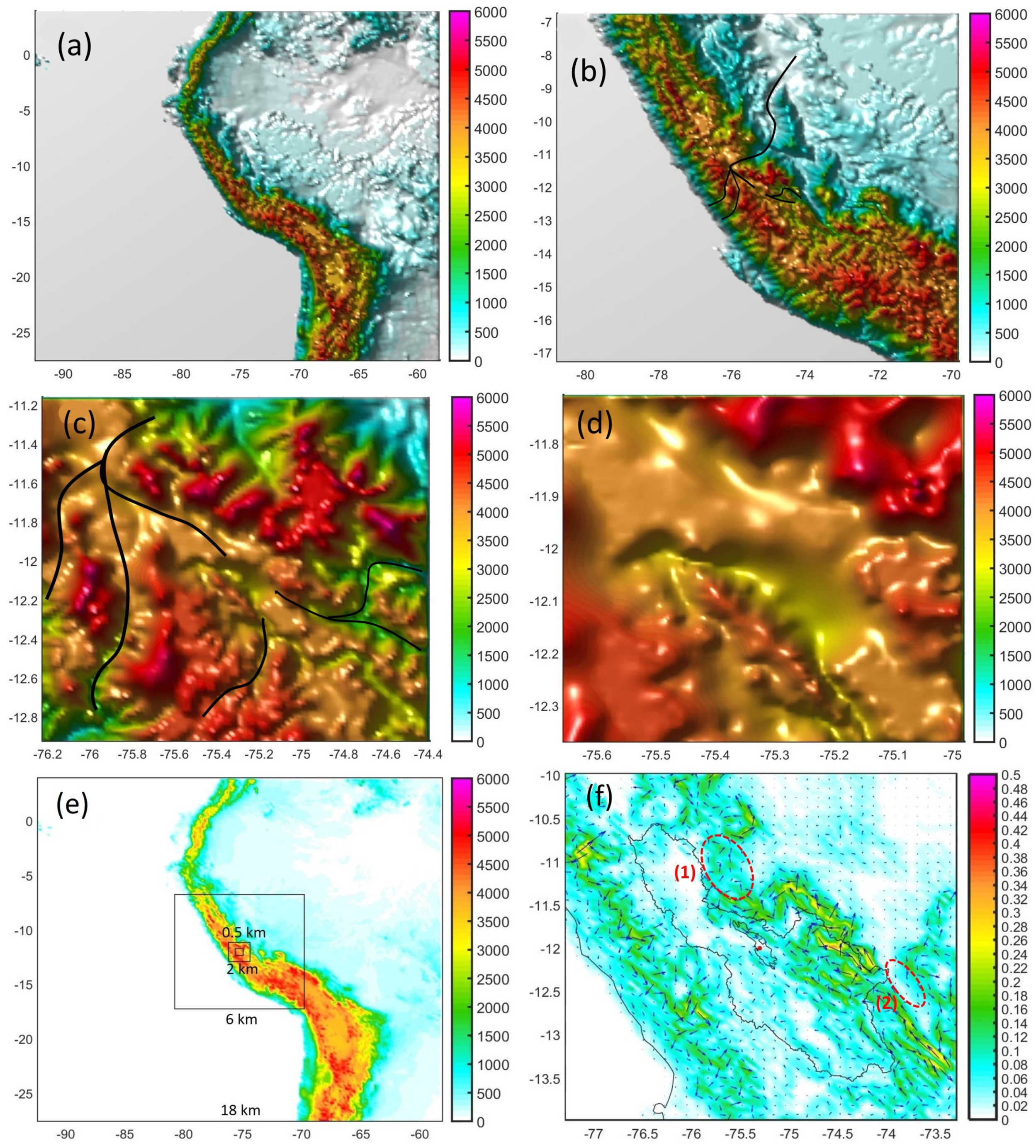
3.2. Numerical Simulations
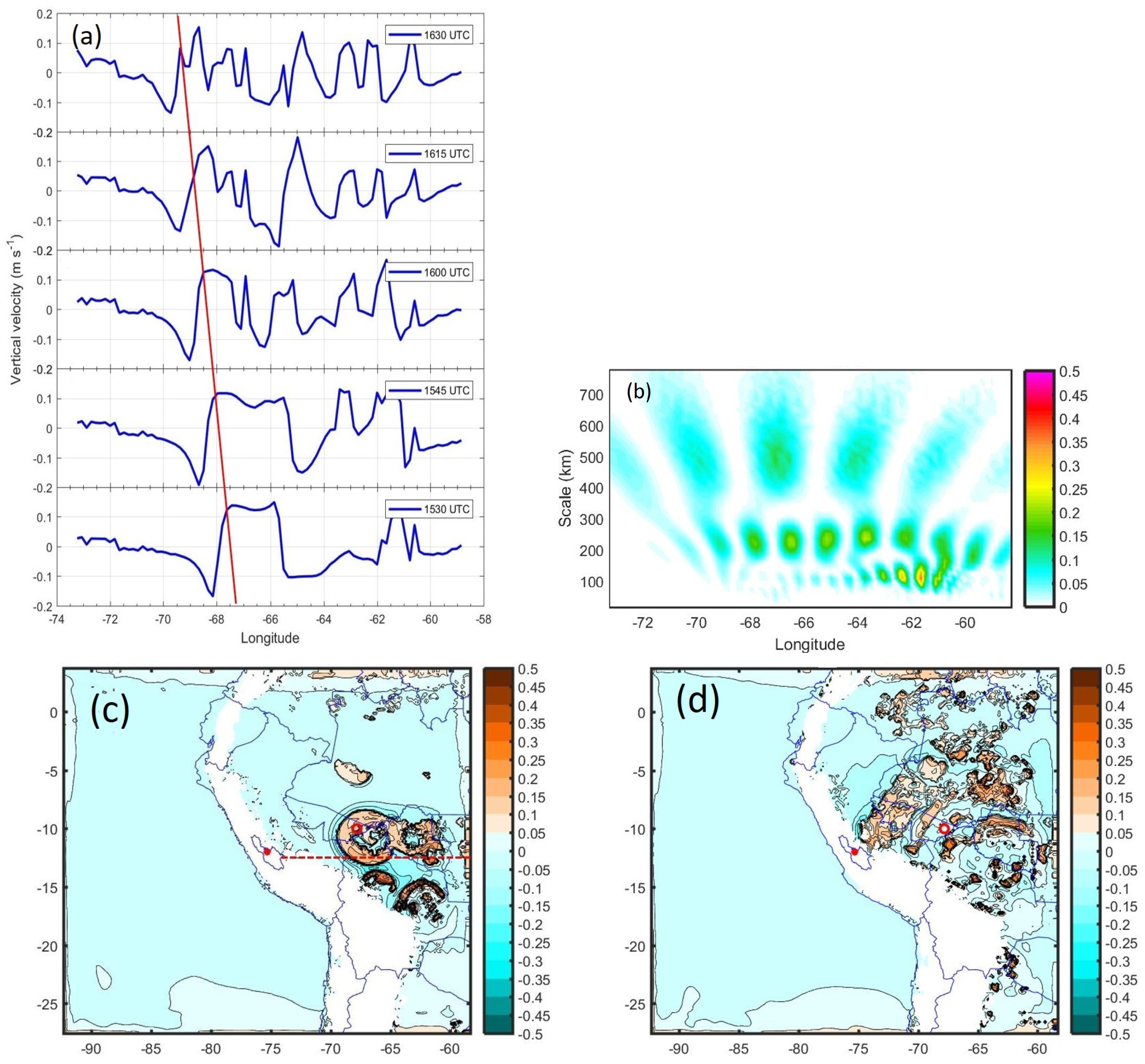
3.3. Wavelet Analysis of Igws
3.4. The Compact Meteorological Ka-Band Cloud Radar (Mira-35c)
3.5. The Boundary Layer and Troposphere Radar (Bltr)
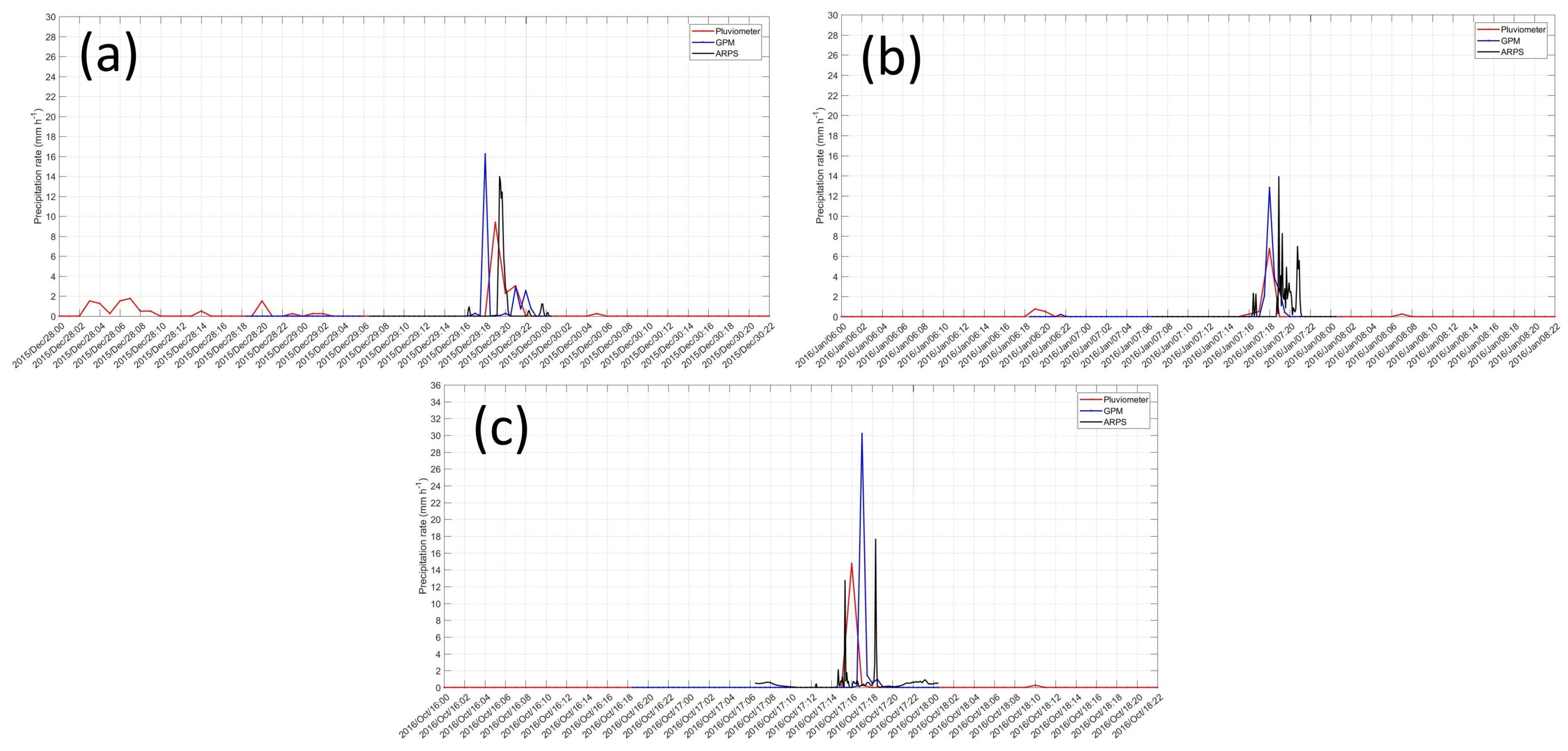
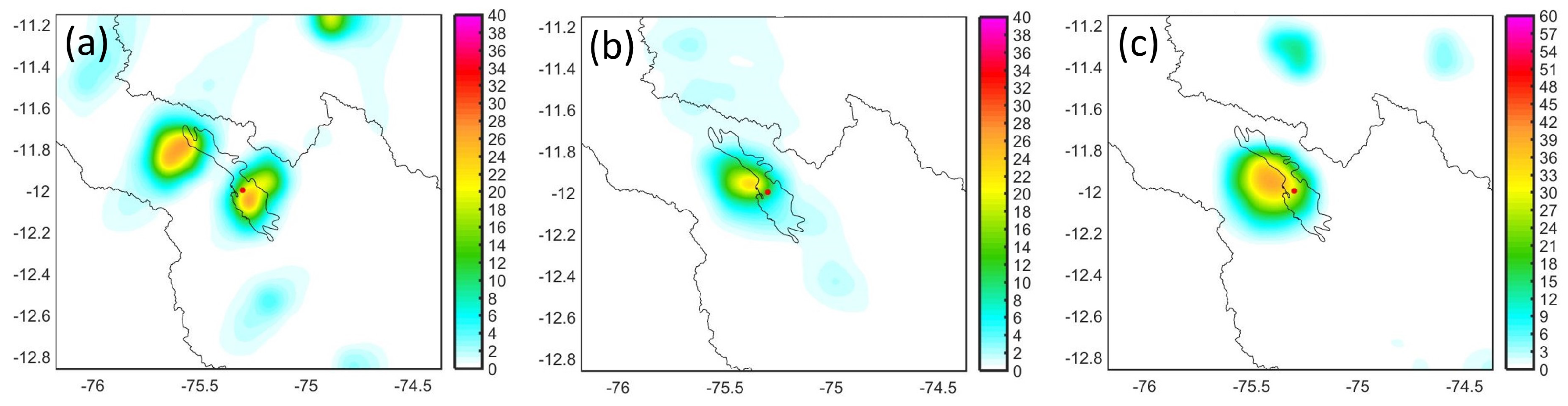
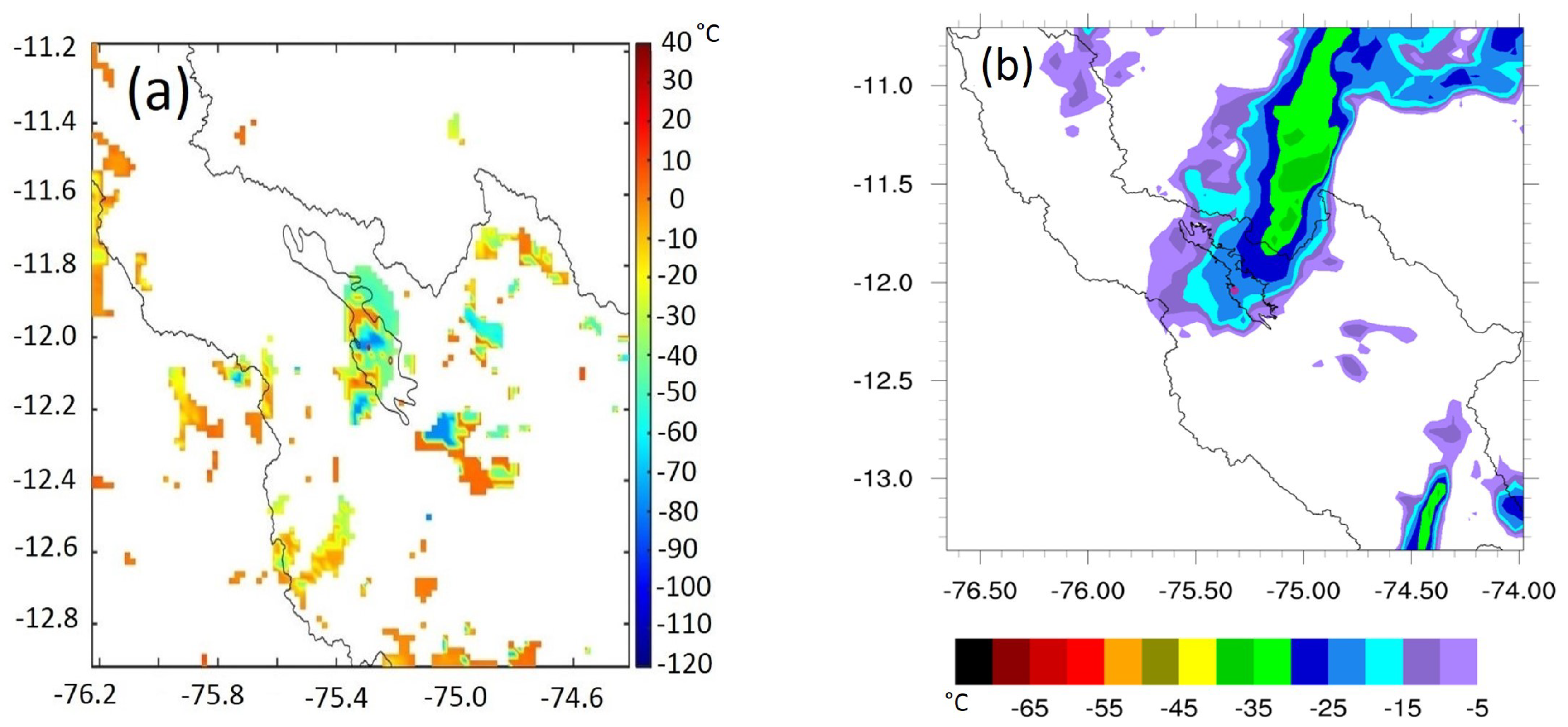
3.6. Global Precipitation Measurement (Gpm), Goes Brightness Temperature and Reanalysis Data
4. Results
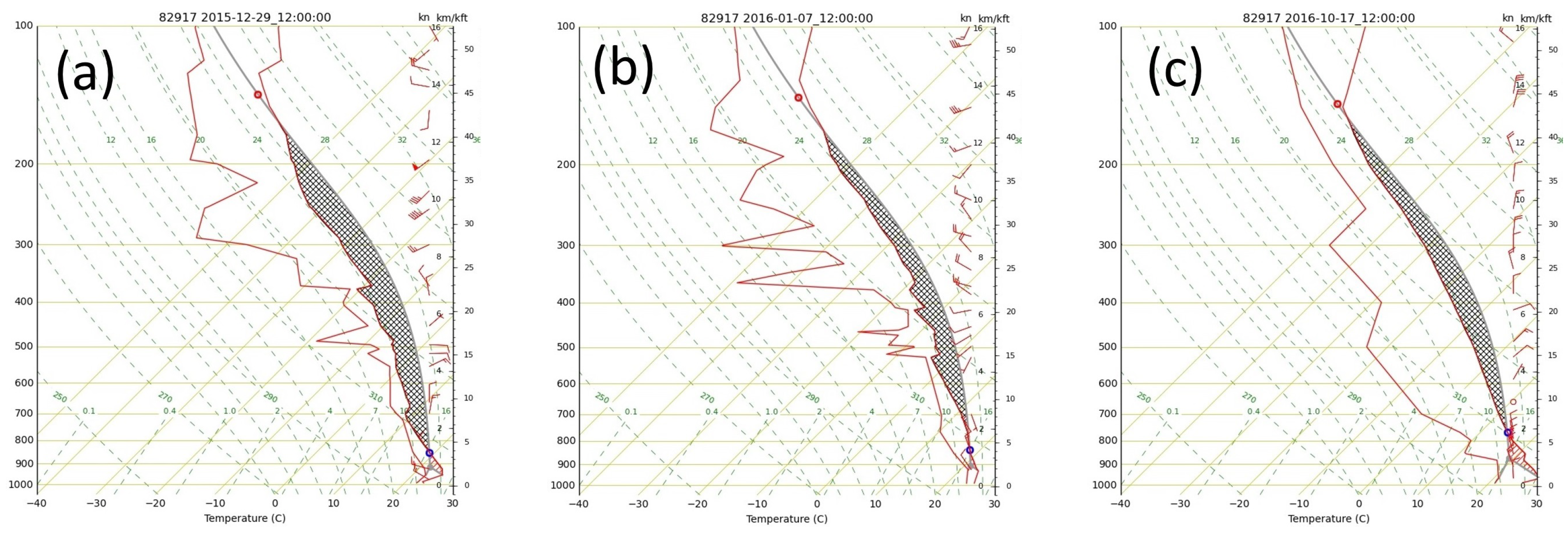
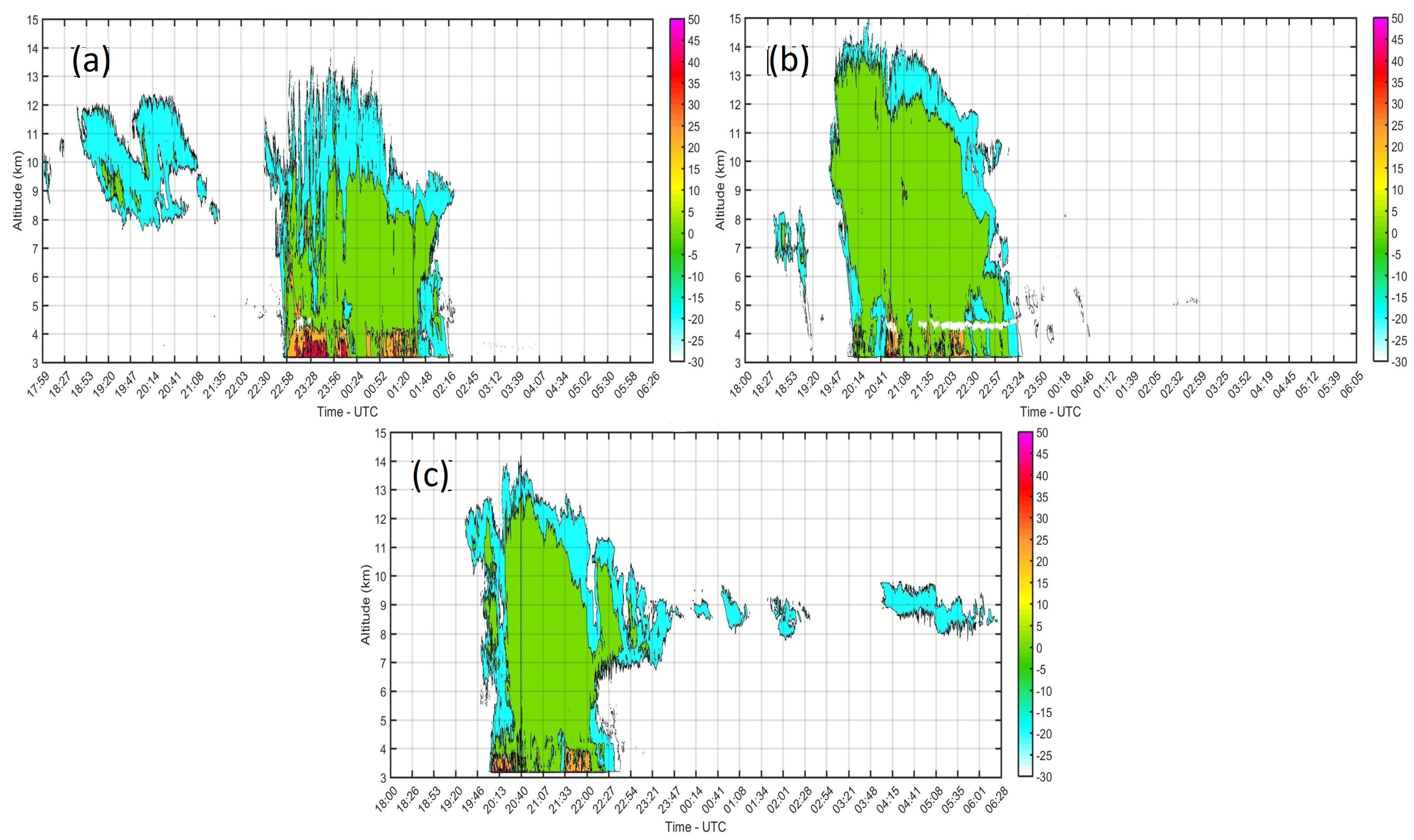
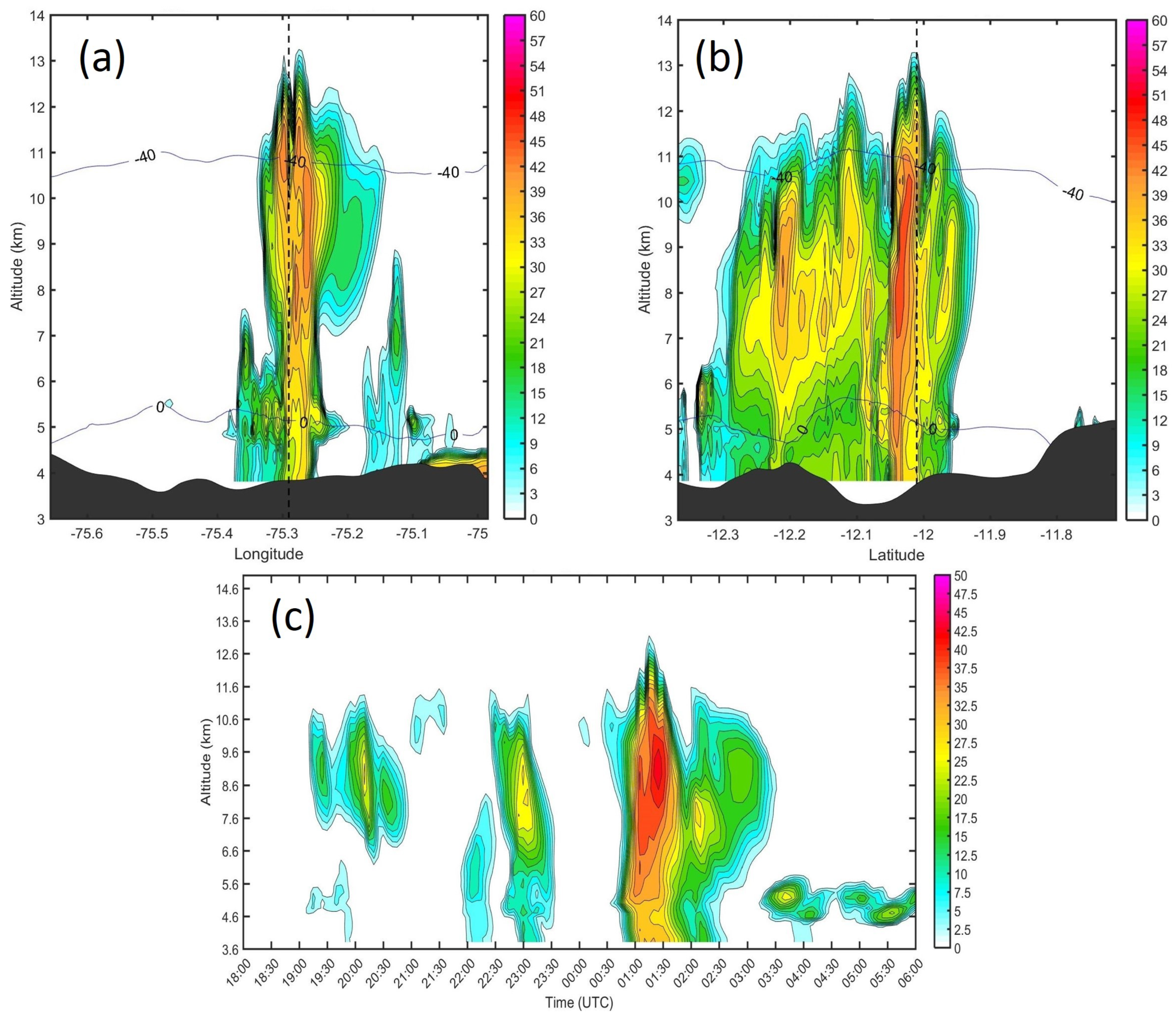
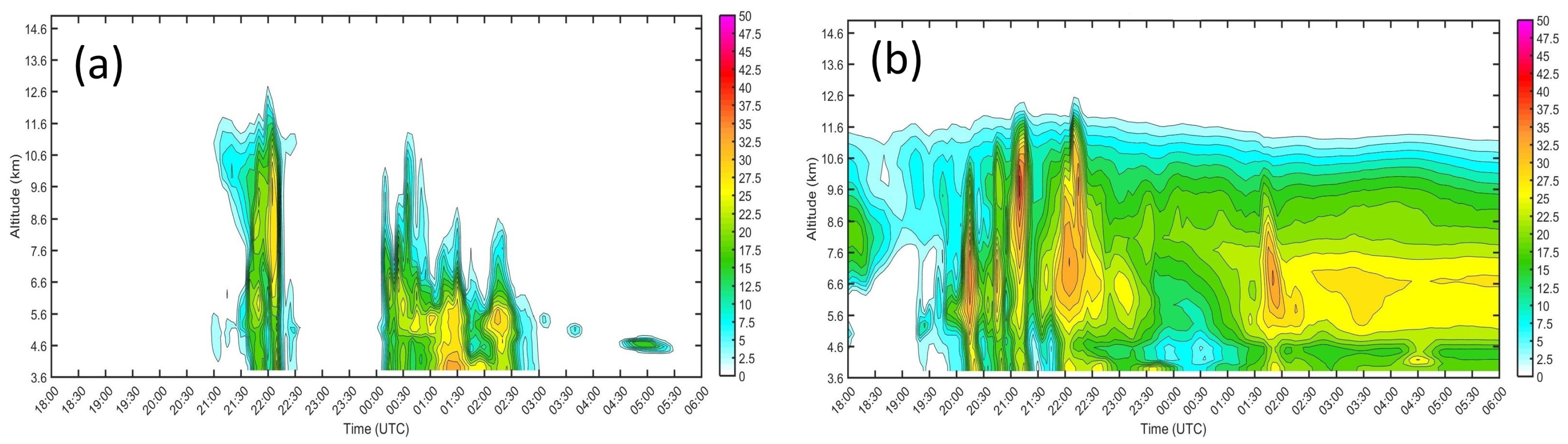
4.1. Observed Data
4.2. Simulation Results
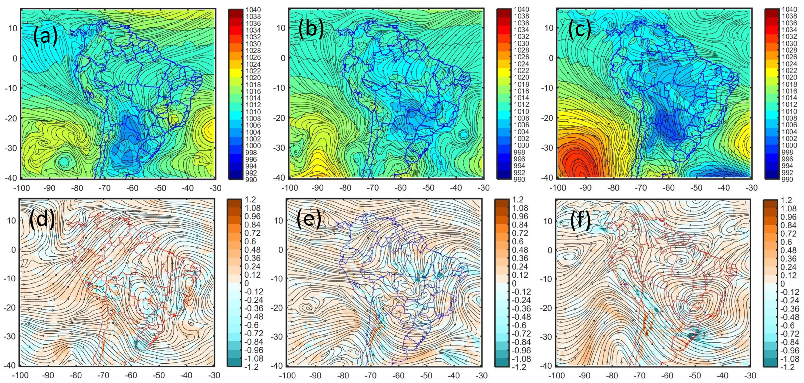
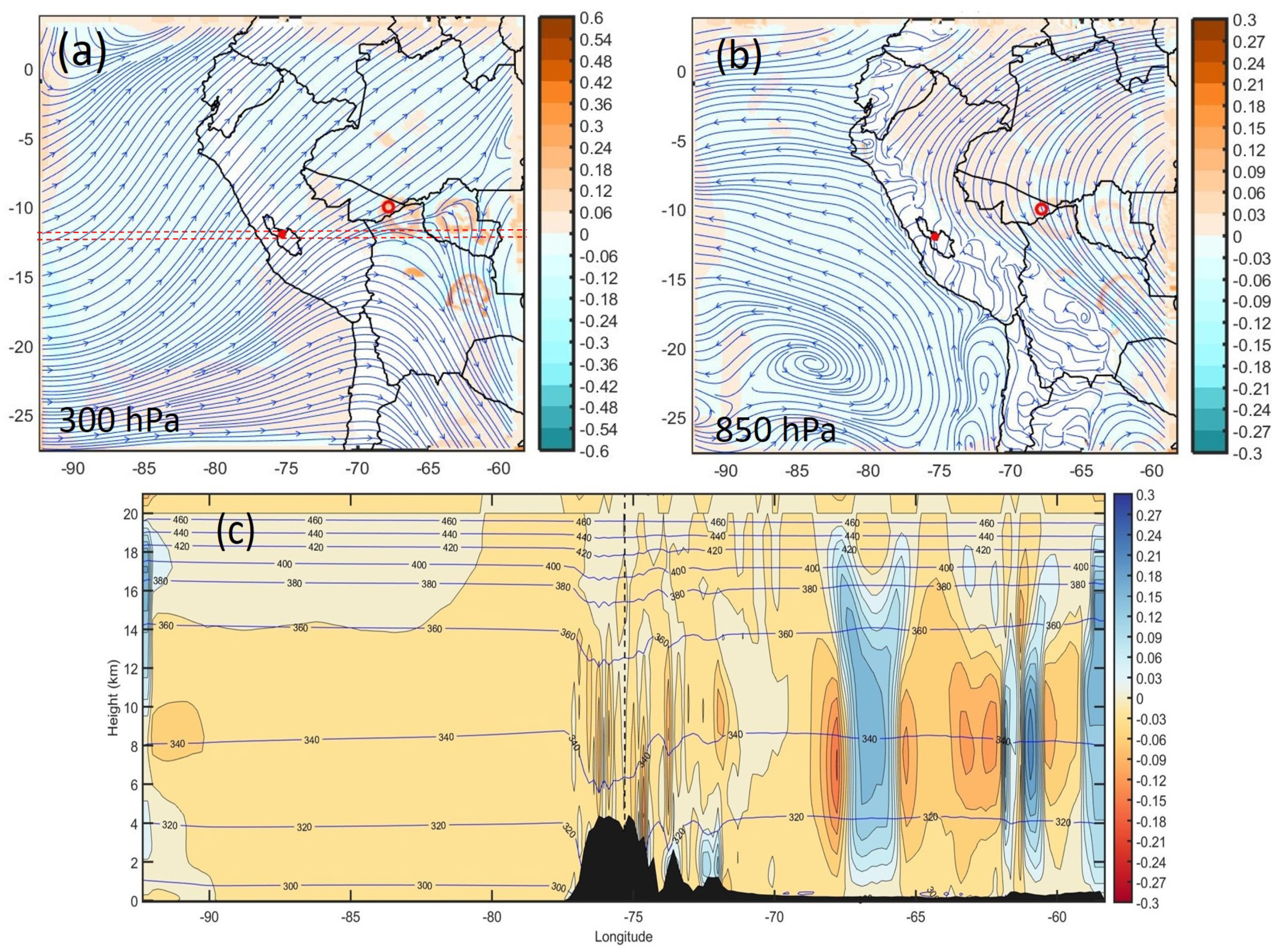
4.2.1. Large Scale Processes
4.2.2. Regional Scale Processes
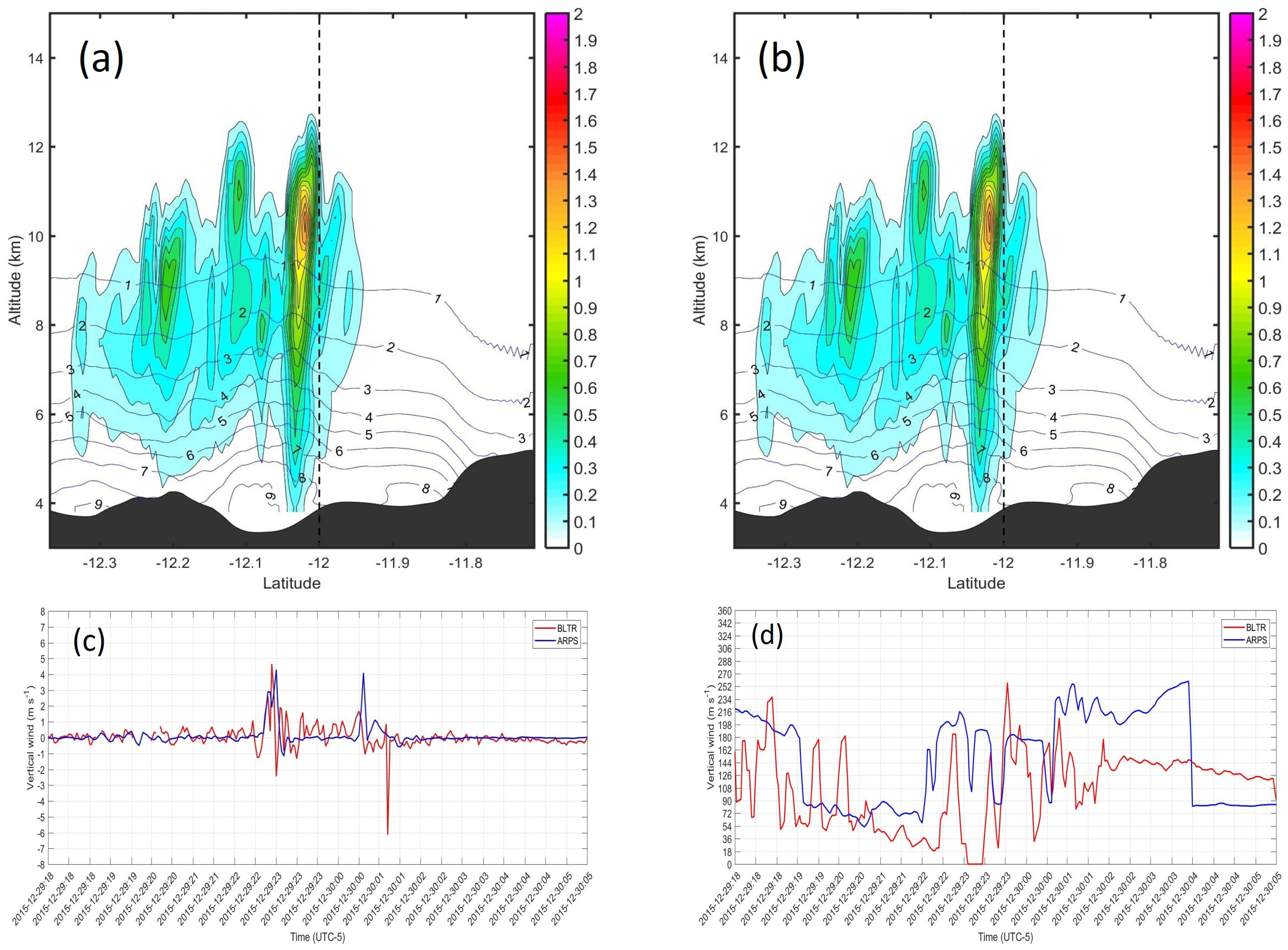
4.2.3. Inertial Gravity Waves
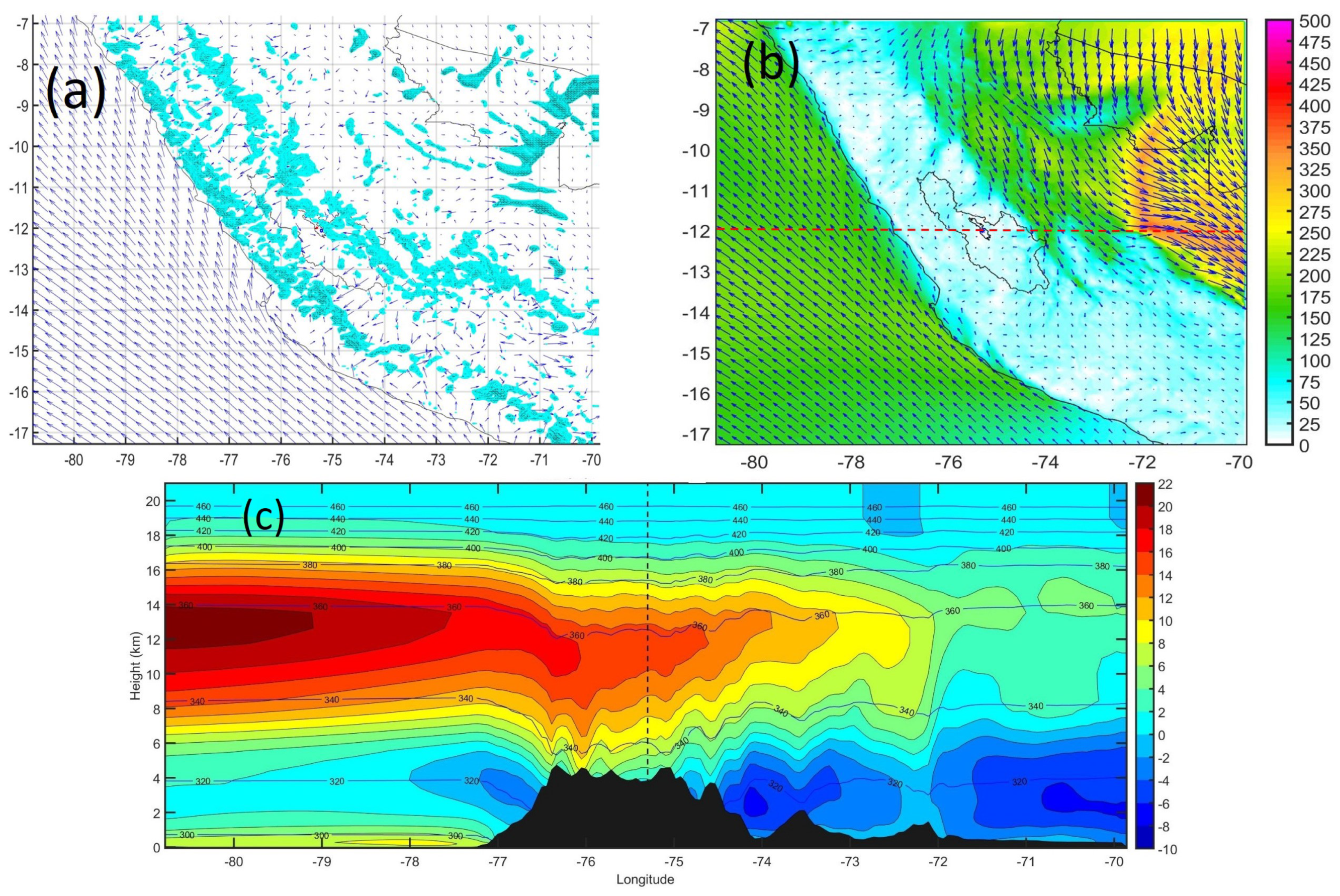
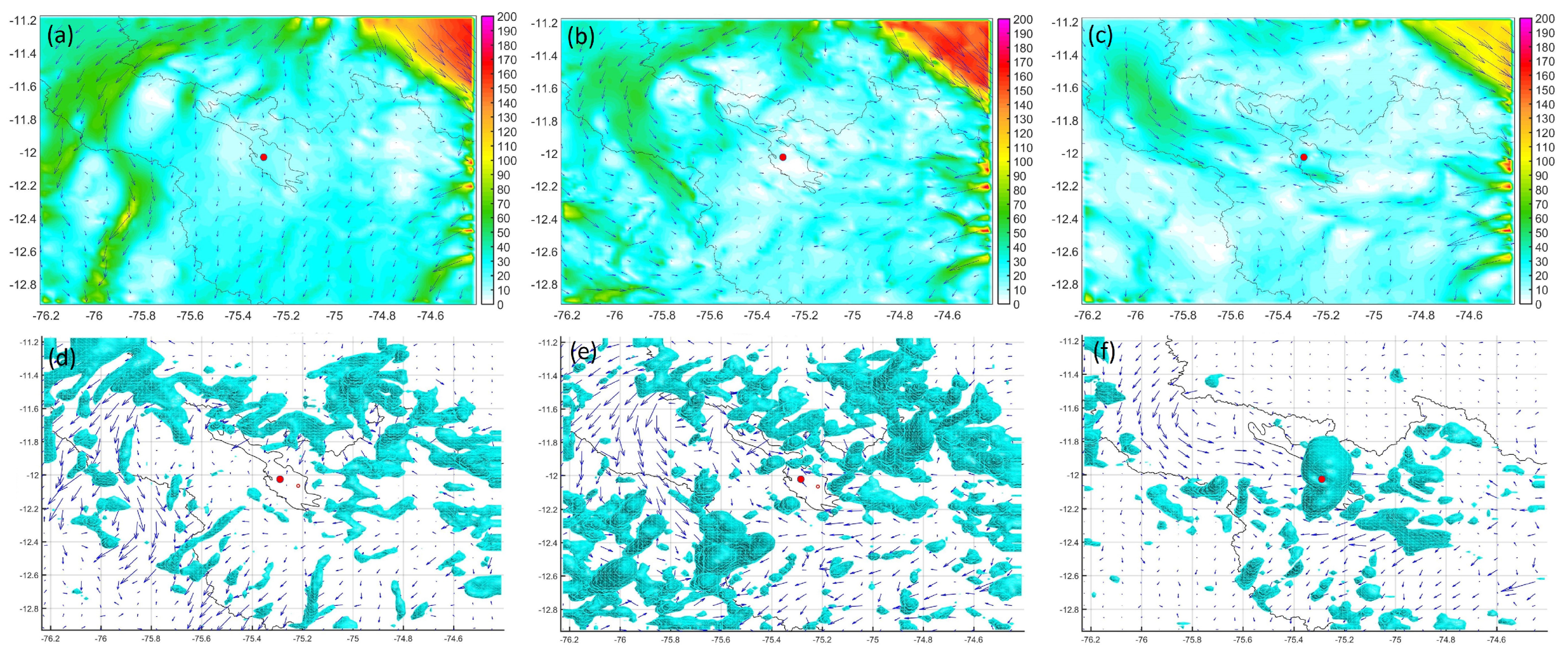
4.2.4. Local Processes
5. Discussions
5.1. Large Scale Processes
5.2. Regional Scale Processes
5.3. Local Scale Processes
6. Conclusions
Author Contributions
Funding
Acknowledgments
Conflicts of Interest
Abbreviations
| ARPS | Advance Regional Prediction system |
| BLTR | Boundary Layer Tropospheric Radar |
| BH-LN | Bolivian high – North east low system |
| Cb | Cumulonimbus |
| CAPE | Convective available potential energy |
| CIN | Convective inhibition energy |
| ECMWF | European Center for Medium-Range Weather Forecasts |
| ENSO | El Niño Southern oscillation |
| GPM | Global Precipitation Measurement |
| GFS | Global Forecast System |
| IGW | Inertial gravity wave |
| MIRA-35c | Compact Meteorological Ka-Band Cloud Radar |
| NCA | Northern Central Andes |
| NCAR | National Center for Atmospheric Research |
| NCEP | National Centers for Environmental Prediction |
| RRTM | Rapid Radiative Transfer Model Longwave |
| SALLJ | South American low level jet |
| SPSA | South-east Pacific Subtropical Anticyclone |
| TSs | Thunderstorms |
| TRMM | Tropical Rainfall Measuring Mission |
| WRF | Weather Research and Forecasting Model |
References
- Cotton, W.; Bryan, G.; Van Den Heever, S. Storm and Cloud Dynamics, 2nd ed.; International Geophysics Series; Elsevier: London, UK, 2011. [Google Scholar]
- Teitelbaum, H.; Le Treut, H.; Moustaqui, M.; Cabrera, G.; Ibañez, G. Deep convection east of the Andes Cordillera: A test case analyses of Airmass origin. Mon. Wea. Rev. 2007, 136, 2201–2209. [Google Scholar] [CrossRef]
- Killeen, T.; Douglas, M.; Consiglio, T.; Jorgensen, P.; Mejia, J. Dry spots and wet spots in the Andean hotspot. J. Biogeogr. 2007, 34, 1357–1373. [Google Scholar] [CrossRef]
- Kumar, S.; Silva-Vidal, Y.; Moya-Álvarez, A.; Martínez-Castro, D. Effect of the surface wind flow and topography on precipitating cloud systems over the Andes and associated Amazon basin: GPM observations. Atmos. Res. 2019, 193–208. [Google Scholar] [CrossRef]
- Andrews, D.; Holton, J.; Leovy, C. Middle Atmosphere Dynamics, 1st ed.; Academic Press: New York, NY, USA, 1987. [Google Scholar]
- Nappo, C. An Introduction to Atmospheric Gravity Waves, 1st ed.; International Geophysics Series; Elsevier Science: San Diego, CA, USA, 2002. [Google Scholar]
- Fritts, D.; Alexander, M. Gravity wave dynamics and effects in the middle atmosphere. Rev. Geophys. 2003, 41. [Google Scholar] [CrossRef] [Green Version]
- Hooke, W. Gravity waves. Mesoscale Meteorology and Forecasting. Am. Meteorol. Soc. 1986, 1, 272–288. [Google Scholar]
- Spiga, A.; Teitelbaum, H.; Zeitlin, V. Identification of the sources of inertia-gravity waves in the Andes Cordillera region. Ann. Geophys. 2008, 26, 2551–2568. [Google Scholar] [CrossRef]
- Qiushi, C. The instability of the gravity-inertia wave and its relation to low-level jet and heavy rainfall. J. Meteorol. Soc. Jpn. 1982, 60, 1041–1056. [Google Scholar]
- Matsumoto, S.; Ninomiya, K. On the meso-scale and medium-scale structure of cold front and relevant vertical circulation. J. Meteorol. Soc. Jpn 1971, 49, 648–668. [Google Scholar] [CrossRef]
- Romatschke, U.; Houze, R., Jr. Extreme Summer Convection in South America. J. Clim. 2010, 23, 3761–3790. [Google Scholar] [CrossRef]
- Egger, J.; Blacutt, L.; Ghezzi, F.; Heinrich, R.; Kolb, P.; Lämmlein, S.; Leeb, M.; Mayer, S.; Palenque, E.; Reuder, J.; et al. Diurnal Circulation of the Bolivian Altiplano. Part I: Observations. Mon. Weather Rev. 2005, 133, 911–934. [Google Scholar] [CrossRef]
- Junquas, C.; Takahashi, K.; Condom, T.; Espinoza, J.; Chavez, S.; Sicart, J.; Lebel, T. Understanding the influence of orography on the precipitation diurnal cycle and the associated atmospheric processes in the central Andes. Clim. Dyn. 2018, 50, 3995–4017. [Google Scholar] [CrossRef]
- Virji, H. A preliminary study of summertime tropospheric circulation patterns overt South America estimated from cloud winds. Mon. Wea. Rev. 1981, 109, 599–612. [Google Scholar] [CrossRef]
- Garreaud, R. Multiscale analysis of the summertime precipitation over the central Andes. Mon. Wea. Rev. 1999, 127, 901–921. [Google Scholar] [CrossRef]
- Garreaud, R.; Vuille, M.; Clement, A. The climate of the Altiplano: Observed and current conditions and mechanisms of past changes. Palaeogeogr. Paleoclimatol. Palaeoecol. 2003, 194, 5–22. [Google Scholar] [CrossRef]
- Falvey, M.; Garreaud, R. Moisture variability over the South American Altiplano during the South American low level jet experiment (SALLJEX) observing season. J. Geophys. Res. 2005, 110, D22105. [Google Scholar] [CrossRef]
- Sulca, J.; Vuille, M.; Silva, Y.; Takahashi, K. Teleconnections between the Peruvian Central Andes and Northeast Brazil during extreme rainfall events in Austral summer. J. Hydrometeorol. 2015, 17, 499–515. [Google Scholar] [CrossRef]
- Vuille, M.; Keimig, F. Interannual variability of summertime convective cloudiness and precipitation in the central Andes derived from ISCCP-B3 data. J. Clim. 2004, 17, 3334–3348. [Google Scholar] [CrossRef]
- Moya-Álvarez, A.; Martínez-Castro, D.; Flores Rojas, J.; Silva Vidal, Y. Sensitivity Study on the Influence of Parameterization Schemes in WRF-ARW Model on Short-and Medium-Range Precipitation Forecasts in the Central Andes of Peru. Adv. Meteorol. 2018, 2018, 1381092. [Google Scholar] [CrossRef]
- IGP. Atlas Climático de Precipitación y Temperatura del Aire en la Cuenca del Río Mantaro, 1st ed.; Fondo Editorial CONAM-Instituto Geofísico del Perú: Lima, Peru, 2005; Volume I. [Google Scholar]
- Simões Reboita, M.; Krusche, N.; Ambrizzi, T.; Porfírio da Rocha, R. Entendendo o Tempo e o Clima na América do Sul. Terra Didatica 2012, 8, 34–50. [Google Scholar] [CrossRef]
- Drumond, A.; Nieto, R.; Gimeno, L.; Ambrizzi, T. A lagrangian identification of major sources of moisture over Central Brazil and La Plata Basin. J. Geophys. Res. 2008, 113, D14128. [Google Scholar] [CrossRef]
- Garreaud, R.; Wallace, J. The diurnal of convective cloudiness over the Americas. Mon. Wea. Rev. 1997, 125, 3157–3171. [Google Scholar] [CrossRef]
- Oke, T. Boundary Layer Climates, 2nd ed.; Taylor and Francis Group: London, UK, 1987. [Google Scholar]
- Wang, M.; Paegle, J. Impact of analysis uncertainty upon regional atmospheric moisture flux. J. Geophys. Res. 1996, 101, 7291–7303. [Google Scholar] [CrossRef]
- Berbery, E.; Collini, E. Springtime Precipitation and Water Vapor Flux over Southeastern South America. Mon. Weather Rev. 1999, 128, 1328–1347. [Google Scholar] [CrossRef]
- Trenberth, K. Climate diagnostics from global analyses: Conservation of mass in ECMWF analyses. J. Clim. 1991, 4, 707–722. [Google Scholar] [CrossRef]
- Connolley, W.; King, J. Atmospheric water vapour transport to Antarctica inferred from radiosondes. J. R. Meteorol. Soc. 1993, 119, 325–342. [Google Scholar] [CrossRef]
- Skamarock, W.C.; Klemp, J.B.; Dudhia, J.; Gill, D.O.; Barker, D.M.; Duda, M.G.; Huang, X.Y.; Wang, W.; Powers, J.G. A Description of the Advanced Research WRF Version 3; National Center For Atmospheric Research, Mesoscale and Microscale Meteorology Division: Boulder, CO, USA, 2008. [Google Scholar]
- Xue, M.; Droegmeier, K.; Wong, V. The Advanced Regional Prediction System (ARPS)-A multi-scale nonhydrostatic atmospheric simulation and prediction model. Part I:Model Dynamics and Verification. Meteorol. Atmos. Phys. 2000, 1, 1–45. [Google Scholar]
- Lin, Y.L.; Farley, R.D.; Orville, H.D. Bulk Parametrization of the Snow Field in a Cloud Model. J. Clim. Appl. Met. 1983, 22, 1065–1092. [Google Scholar] [CrossRef]
- Ek, M.; Mitchell, K.; Lin, Y.; Rogers, E.; Grummann, P.; Koren, V.; Gayno, G.; Tarpley, J. Implementation of Noah land surface model advances in the National Centers for Environmental Prediction operational Mesoscale Eta Model. J. Geophys. Res. 2003, 108, 8851. [Google Scholar] [CrossRef]
- Tewari, M.; Chen, F.; Wang, W.; Dudhia, J.; LeMone, M.; Mitchell, K.; Ek, M.; Gayno, G.; Wegiel, J.; Cuenca, R. Implementation and verification of the unified NOAH land surface model in the WRF model. In Proceedings of the 20th Conference on Weather Analysis and Forecasting/16th Conference on Numerical Weather Prediction, Seattle, WA, USA, 10 January 2004. [Google Scholar]
- Monin, A.; Obukhov, A. Basic laws of turbulent mixing in the surface layer of the atmosphere. Trans. Geophys. Inst. Akad. Nauk. USSR 1954, 151, 163–187. [Google Scholar]
- Grell, G.; Freitas, S. A scale and aerosol aware stochastic convective parameterization for weather and air quality modeling. Atmos. Chem. Phys. 2014, 13, 23845–23893. [Google Scholar] [CrossRef]
- Hong, S.; Noh, Y.; Dudhia, J. A new vertical diffusion package with an explicit treatment of entrainment processes. Mon. Weather Rev. 2006, 134, 2318–2341. [Google Scholar] [CrossRef]
- Mlawer, E.J.; Taubman, S.J.; Brown, P.D.; Iacono, M.J.; Clough, S.A. Radiative transfer for inhomogeneous atmospheres: RRTM, a validated correlated-k model for the longwave. J. Geophys. Res. 1997, 102, 16663–16682. [Google Scholar] [CrossRef] [Green Version]
- Xue, M.; Droegmeier, K.; Wong, V. The Advanced Regional Prediction System (ARPS)-A multi-scale nonhydrostatic atmospheric simulation and prediction model. Part II: Model physics and applications. Meteorol. Atmos. Phys. 2001, 76, 143–165. [Google Scholar] [CrossRef]
- Schultz, P. An explicit cloud physics paramterization for operational numerical weather prediction. Mon. Weather Rev. 1995, 123, 3331–3343. [Google Scholar] [CrossRef]
- De la Torre, A.; Alexander, P.; Llamedo, P.; Menéndez, C.; Schmidt, T.; Wickert, J. Gravity waves above the Andes detected from GPS radio occultation temperature profiles: Jet mechanism? Geophys. Res. Lett. 2006, 33, 248–258. [Google Scholar] [CrossRef]
- De la Torre, A.; Hierro, R.; Llamedo, P.; Rolla, A.; Alexander, P. Severe hailstorms near Southern Andes in the presence of mountain waves. Atmos. Res. 2010, 101, 112–123. [Google Scholar] [CrossRef]
- Shutts, G.; Kitchen, M.; Hoare, P. A large amplitude gravity wave in the lower stratosphere detected by radiosonde. Q. J. R. Meteorol. Soc. 1988, 114, 579–594. [Google Scholar] [CrossRef]
- Claret, M.; Viúdez, A. Vertical velocity in the interaction between inertia-gravity waves and submesoscale baroclinic vortical structures. J. Geophys. Res. 2010, 115, 2156–2202. [Google Scholar] [CrossRef]
- Metek. MIRA-35c System Description; Meteorologische Messtechnik GmbH: Elmshorn, Germany, 2015. [Google Scholar]
- Sokol, Z.; Minárová, J.; Novák, P. Classification of Hydrometeors Using Measurements of the Ka-Band Cloud Radar Installed at the Milesovka Mountain (Central Europe). Remote Sens. 2018, 10, 1674. [Google Scholar] [CrossRef]
- Scipión, D.; Palmer, R.; Chilson, P.; Fedorovich, E.; Botnick, A. Retrieval of convective boundary layer wind field statistics from radar profiler measurements in conjunction with large eddy simulation. Meteorol. Z. 2009, 18, 175–187. [Google Scholar] [CrossRef]
- Scipión, D.; Palmer, R.; Chilson, P.; Fedorovich, E.; Botnick, A. Turbulence kinetic energy and dissipation rate estimated from a virtual wind profiles and verified trhough large eddy simualations. In Proceedings of the 34th AMS Conference on Radar Meteorology, Williamsburg, VA, USA, 5–9 October 2009; pp. 1–14. [Google Scholar]
- Prakash, S.; Mitra, A.K.; Pai, D.; AghaKouchak, A. From TRMM to GPM: How well can heavy rainfall be detected from space? Adv. Water Res. 2016, 88, 1–7. [Google Scholar] [CrossRef]
- Guo, H.; Chen, S.; Bao, A.; Behrangi, A.; Hong, Y.; Ndayisaba, F.; Hu, J.; Stepanian, P. Early assessment of integrated multi-satellite retrievals for global precipitation measurement over China. Atmos. Res. 2016, 176–177, 121–133. [Google Scholar] [CrossRef]
- Ma, Y.; Tang, G.; Long, D.; Yong, B.; Zhong, L.; Wan, W.; Hong, Y. Similarity and error intercomparison of the GPM and its predecessor-TRMM multisatellite precipitation analysis using the best available hourly gauge network over the Tibetan Plateau. Remote Sens. 2016, 8, 569. [Google Scholar] [CrossRef]
- Tang, G.; Zeng, Z.; Long, D.; Guo, X.; Yong, B.; Zhang, W.; Hong, Y. Statistical and hydrological comparisons between TRMM and GPM Level-3 products over a midlatitude basin: Is Day-1 IMERG a good successor for TMPA 3B42v7? J. Hydrometeorol. 2016, 17, 121–137. [Google Scholar] [CrossRef]
- Chen, C. The convective instability of the inertia wave and physical analysis of the formation of the typhoon in the early stage. Acta Met. Sin. 1964, 34, 433–442. [Google Scholar]
- Sharifi, E.; Steinacker, R.; Saghafian, B. Assessment of GPM-IMERG and other precipitation products against gauge data under different topographic and climatic conditions in Iran: Preliminary results. Remote Sens. 2016, 8, 135. [Google Scholar] [CrossRef]
- Tan, J.; Petersen, W.; Tokay, A. A novel approach to identify sources of errors in IMERG for GPM ground validation. J. Hydrometeorol. 2016, 17, 2477–2491. [Google Scholar] [CrossRef]
- Hobouchian, M.; Salio, P.; García Skabar, Y.; Vila, D.; Garreaud, R. Assessment of satellite precipitation estimates over the slopes of the subtropical Andes. Atmos. Res. 2017, 190, 43–54. [Google Scholar] [CrossRef]
- Manz, B.; Páez-Bimos, S.; Horna, N.; Buytaert, W.; Ochoa-Tocachi, B.; Lavado-Casimiro, W.; Willems, B. Comparative Ground Validation of IMERG and TMPA at Variable Spatiotemporal Scales in the Tropical Andes. J. Hydrometeorol. 2017, 18, 2469–2489. [Google Scholar] [CrossRef]
- Menzel, W.P.; Purdom, J.F. Introducing GOES-I: The first of a new generation of geostationary operational environmental satellites. Bull. Am. Meteorol. Soc. 1994, 75, 757–781. [Google Scholar] [CrossRef]
- Lhermitte, R. Attenuation and Scattering of Millimeter Wavelength Radiation by Clouds and Precipitation. J. Atmos. Ocean. Technol. 1990, 7, 464–479. [Google Scholar] [CrossRef] [Green Version]
- Chavez, S.; Takahashi, K. Orographic rainfall hot spots in the Andes-Amazon transition according to the TRMMM precipitation radar and in situ data. J. Geophys. Res. Atmos. 2017, 122, 5870–5882. [Google Scholar] [CrossRef]
- Kalthoff, N.; Bischoff-Gaub, I.; Fiedler, F. Mesoscale wind regimes in Chile at 30°. J. Appl. Meteorol. 2002, 41, 953–970. [Google Scholar] [CrossRef]
- Garreaud, R. The Andes climate and weather. Adv. Geosci. 2009, 22, 3–11. [Google Scholar] [CrossRef] [Green Version]
- Barry, R.G. Mountain Weather and Climate, 3rd ed.; Cambridge, University Press: New York, NY, USA, 2008; p. 73. [Google Scholar]
- Guest, F.; Reeder, M.; Marks, C.; Karoly, D. Inertia-gravity waves observed in the lower stratosphere over Macquarie Island. J. Atmos. Sci. 2000, 57, 737–752. [Google Scholar] [CrossRef]
- Pavelin, E.; Whiteway, J.A.; Vaughan, G. Observation of gravity wave generation and breaking in the lowermost stratosphere. J. Geophys. Res. 2001, 106, 5173–5180. [Google Scholar] [CrossRef]
- Plougonven, R.; Teitelbaum, H.; Zeitlin, V. Inertia gravity wave generation by the tropospheric midlatitude jet as given by the Fronts and Atlantic Storm-Track Experiment radio soundings. J. Geophys. Res. 2003, 108, 4686–4704. [Google Scholar] [CrossRef]
- Kessler, E. On the Distribution and Continuity of Water Substance in Atmospheric Circulations. Meteorol. Monogr. 1969, 10, 1–88. [Google Scholar]
- Ancapichún, S.; Garcés-Vargas, J. Variability of the Southeast Pacific Subtropical Anticyclone and its impact on sea surface temperature off north-central Chile. Cienc. Mar. 2015, 41, 1–20. [Google Scholar] [CrossRef] [Green Version]
- Houston, J.; Hartley, A. The central Andean west-slope rain-shadow and its potentical contribution to the origin of hyperaridity in the Atacama Desert. Int. J. Climatol. 2003, 23, 1453–1464. [Google Scholar] [CrossRef]
- Marengo, J.; Soares, W.; Saulo, C.; Nicolini, M. Climatology of the Low-Level Jet East of the Andes as Derived from the NCEP–NCAR Reanalyses: Characteristics and Temporal Variability. J. Clim. 2004, 17, 2261–2280. [Google Scholar] [CrossRef]
- Vera, C.; Baez, J.; Douglas, M.; Emmanuel, C.; Marengo, J.; Meitin, J.; Nicolini, M.; Nogues-Paegle, J.; Paegle, J.; Penalba, O.; et al. The South American Low-Level Jet Experiment. Bull. Am. Meteorol. Soc. 2006, 87, 63–77. [Google Scholar] [CrossRef]
- Lenters, J.; Cook, K. On the origin of the Bolivian high and related circulation features of the South American climate. J. Atmos. Sci. 1997, 54, 656–677. [Google Scholar] [CrossRef]
- Pereira Filho, A.; Barros, M.; Hallak, R.; Gandu, A. Enchentes na região metropilitana de São Paulo: Aspectos de mesoescala e avaliação de impactos. In Proceedings of the XIII Congresso Brasileiro de Meterologia, Fortaleza, CE, USA, 28 August–3 September 2004. [Google Scholar]
- Vemado, F.; Pereira Filho, A. Severe weather caused by Heat Island and Sea breeze effects in the Metropolitan Area of São Paulo, Brazil. Adv. Meteorol. 2015, 2016, 8364134. [Google Scholar] [CrossRef]
- Fett, R.; Tag, P. Satellite observation and numerical model results of sea breeze effects as applied to the west coast of South America. In Proceedings of the First International conference on Southern Hemisphere Meteorology, São José dos Campos, Brazil, 31 July–6 August 1983; pp. 337–340. [Google Scholar]
- Horel, J.; Cornejo-Garrido, A. Convection along the coast of northern Peru during 1983. Mon. Weather Rev. 1986, 114, 2091–2105. [Google Scholar] [CrossRef]
- Takahashi, K. The atmospheric circulation associated with the extreme rainfall events in Piura, Peru, during the 1997 and 2002 El niño events. Ann. Geophys. 2004, 22, 3917–3926. [Google Scholar] [CrossRef]
- Bendix, J. Precipitation dynamics in Ecuador and northern Peru during the 1991/92 El niño: A remote sensing perspective. Int. J. Remote Sens. 2000, 21, 533–548. [Google Scholar] [CrossRef]
- Espinoza, J.; Chavez, S.; Ronchail, J.; Junquas, C.; Takahashi, K.; Lavado, W. Rainfall hotspots over the southern tropical Andes: Spatial distribution, rainfall intensity and relations with large-scale atmospheric circulation. Water Resour. Res. 2015, 51, 1–17. [Google Scholar] [CrossRef]
- Flohn, H. Hochgebirge und allgemeine Zirkulation II. Die Gebirge als Warmequellen. Arch. Meteorol. Geophys. Biokl. 1953, A5, 265–279. [Google Scholar]
- Houze, R. Cloud Dynamics, 1st ed.; Academic Press: San Diego, CA, USA, 1993. [Google Scholar]


© 2019 by the authors. Licensee MDPI, Basel, Switzerland. This article is an open access article distributed under the terms and conditions of the Creative Commons Attribution (CC BY) license (http://creativecommons.org/licenses/by/4.0/).
Share and Cite
J.L., F.R.; A.S., M.-A.; S., K.; D., M.-C.; E., V.-P.; Y., S.-V. Analysis of Possible Triggering Mechanisms of Severe Thunderstorms in the Tropical Central Andes of Peru, Mantaro Valley. Atmosphere 2019, 10, 301. https://doi.org/10.3390/atmos10060301
J.L. FR, A.S. M-A, S. K, D. M-C, E. V-P, Y. S-V. Analysis of Possible Triggering Mechanisms of Severe Thunderstorms in the Tropical Central Andes of Peru, Mantaro Valley. Atmosphere. 2019; 10(6):301. https://doi.org/10.3390/atmos10060301
Chicago/Turabian StyleJ.L., Flores Rojas, Moya-Alvarez A.S., Kumar S., Martinez-Castro D., Villalobos-Puma E., and Silva-Vidal Y. 2019. "Analysis of Possible Triggering Mechanisms of Severe Thunderstorms in the Tropical Central Andes of Peru, Mantaro Valley" Atmosphere 10, no. 6: 301. https://doi.org/10.3390/atmos10060301