An Assessment of Coordinate Rotation Methods in Sonic Anemometer Measurements of Turbulent Fluxes over Complex Mountainous Terrain

Abstract

The measurement of turbulent fluxes in the atmospheric boundary layer is usually performed using fast anemometers and the Eddy Covariance technique. This method has been applied here and investigated in a complex mountainous terrain. A field campaign has recently been conducted at Alpe Veglia (the Central-Western Italian Alps, 1746 m a.s.l.) where both standard and micrometeorological data were collected. The measured values obtained from an ultrasonic anemometer were analysed using a filtering procedure and three different coordinate rotation procedures: Double (DR), Triple Rotation (TR) and Planar Fit (PF) on moving temporal windows of 30 and 60 min. A quality assessment was performed on the sensible heat and momentum fluxes and the results show that the measured turbulent fluxes at Alpe Veglia were of a medium-high quality level and rarely passed the stationary flow test. A comparison of the three coordinate procedures, using quality assessment and sensible heat flux standard deviations, revealed that DR and TR were comparable, with significant differences, mainly under low-wind conditions. The PF method failed to satisfy the physical requirement for the multiple planarity of the flow, due to the complexity of the mountainous terrain.

1. Introduction

High mountain environments are rapidly changing as a result of the ongoing climate changes, which are quickly modifying not only landscapes but also ecological components, such as vegetation, including flora and fauna, as well as human fruition and geoheritage [1]. In mountain areas, glacier shrinkage is accompanied by a widening of the proglacial areas ([2] and reference herein), while some debris-free glaciers are transforming into debris covered ones and a transition is occurring from glacial to paraglacial systems [3]. Debris covered glaciers are progressively being colonized by supraglacial grass, shrubs and trees [4] and new biological successions are emerging [5].

The nearest atmospheric layer to the surface is the Atmospheric Boundary Layer (ABL), where exchanges of momentum, mass and energy with the surface take place. Its structure is more complex in mountain environments than over flat, horizontal and homogeneous terrains and it has a multi-layered configuration due to transport processes, which interact at different spatial and temporal scales. In mountain environments, some authors have defined a specific ABL as a Mountain Boundary Layer (MBL) [6].

Better knowledge of land surface exchanges over complex terrains [6], and in particular over mountainous terrains [7], which represent an extreme case of high complexity because of the steep slopes and frequent characteristic land-surface changes, could contribute to describing the general evolution of high mountain environments.

Unfortunately, there are few monitoring stations in this area and there are even fewer stations equipped with fast instruments. Accurate measurements of the energy and mass fluxes on the surface of complex terrains are also important because they may be used to validate the surface schemes in meteorological forecasting models, which may be more difficult to use in complex terrain environments.

Turbulent quantities are usually measured using fast response instrumentation that is able to capture the behaviour of turbulent air flows. The main instruments are ultrasonic anemometers, which measure turbulence variables and allow turbulent quantities to be computed from high frequency measurements (from 10 $\mathrm{Hz}$) that is the three components of the wind speed and the speed of sound. In order to obtain mean values, fluctuations, covariances and fluxes, the data need to be rotated from the anemometer coordinate reference system to a streamline coordinate system [8]. Three main coordinate rotation methods exist: Double Rotation (DR, [9]), Triple Rotation (TR, [10]) and Planar Fit (PF, [11,12]). Wind data are acquired in an ultrasonic anemometer reference system, as mentioned above, which usually has an x-axis directed towards the East, a y-axis directed towards the North and a z-axis perpendicular and facing the zenith. The DR method rotates this reference system with two rotations around the z and y axes, and positions the mean wind value on the x-axis. The TR method performs a third rotation around the x-axis, and positions the z-axis perpendicular to the streamline surface. Rotations are generally applied over a fixed short-time interval of 30 or 60 min. The PF method, instead, computes a mean plane using the complete dataset (more than 15 days), where the mean vertical wind component is zero. The x-y plane of the reference system is then placed on the PF plane with the x-axis along the mean wind direction.

These techniques have been applied successfully over flat, horizontal and homogeneous terrain in several measurement campaigns (among others: [13,14]). They have also been used over non-homogeneous and sloped terrains in a number of different applications, such as in agrometeorological studies [15], for complex urban and sub-urban terrains [16], and for mountainous terrain measurements [17]. This paper presents an evaluation of the performances of the three rotation methods over high altitude mountainous terrain in an area of extreme complexity.

For this purpose, a micrometeorological station was set up in a mountain environment in the Central-Western Italian Alps, on an alluvial plain lying over a glacio-tectonic depression [18], surrounded by high mountain peaks. The station was equipped with traditional instrumentation and an ultrasonic anemometer to measure turbulence. The ultrasonic anemometer data were filtered following a procedure derived from literature and analysed using the Eddy Covariance method and the three aforementioned coordinate rotation methods (DR, TR and PF). Finally, on the previously filtered data, two similar procedures were applied to evaluate the goodness of coordinate rotation methods: the data-quality assessment procedure following Stiperski and Rotach (2016) [19] and the standard deviation calculation on fluxes, evaluated after Wyngaard (1973) [20].

The results are presented and discussed with the aim of evaluating whether the three methods, which were designed for flat, horizontal and homogeneous terrain, are suitable for computing surface fluxes over complex terrain.

2. Materials and Methods

2.1. Description of the Experiment

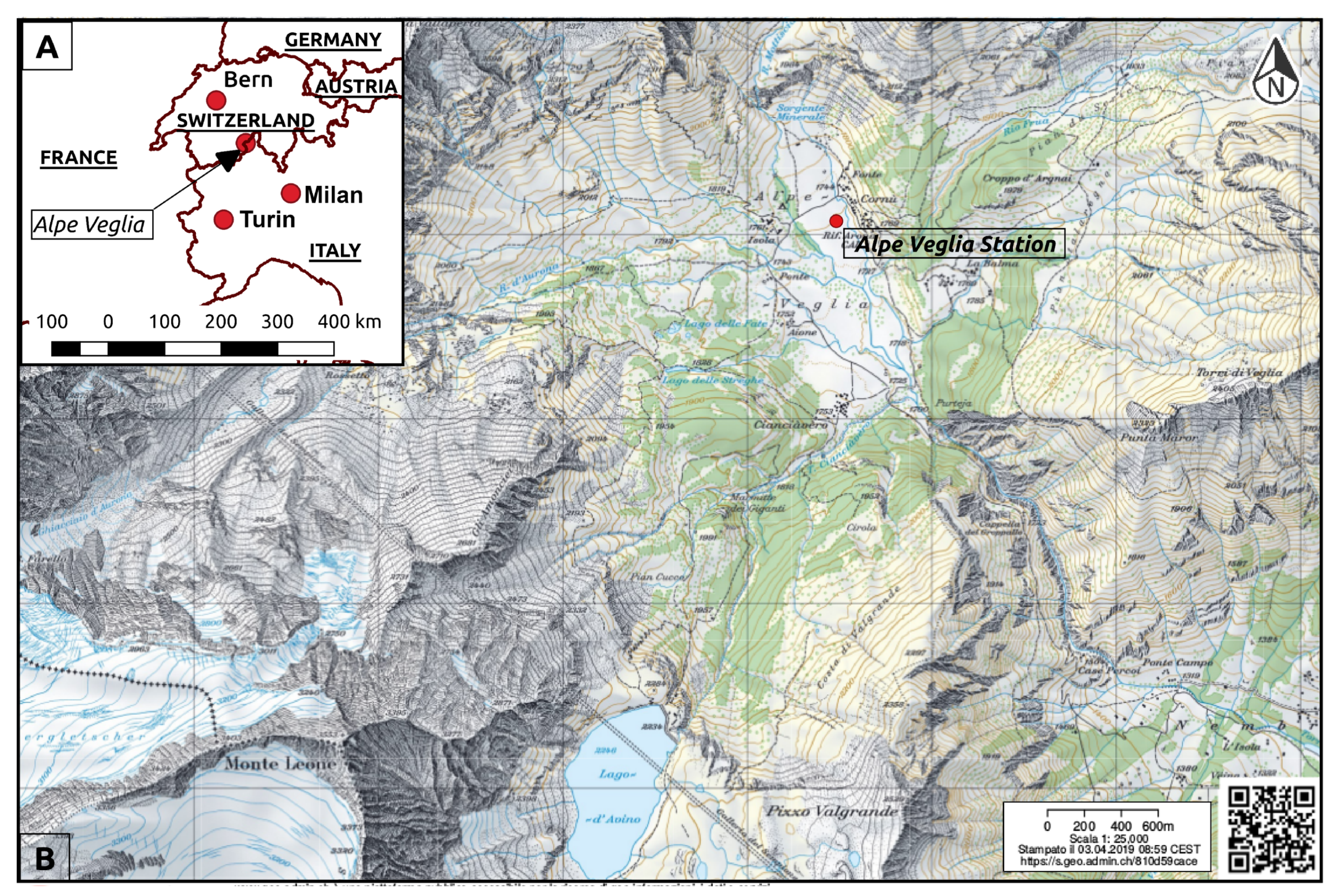
A micrometeorological station was installed at Alpe Veglia in the municipality of Varzo (Verbano Cusio Ossola) at 1746 $\mathrm{m}$ a.s.l. (long: 8°8′44.46″ E, lat: 46°16′38.48″ N, WGS84), in the Central-Western Italian Alps (Lepontine Alps), near the Simplon Pass at the border between Italy and Switzerland (Figure 1). The experiment was started on 27 September 2018, and the data analysed in this paper span from the beginning of the campaign to 16 November 2018, when the first data retrieval was performed, and the station was prepared for the winter season. Overall, the dataset is composed of 49 complete days.

The station is located in an alluvial plain lying over a glacio-tectonic depression (Alpe Veglia plain) [18]. The installation area is surrounded by high mountain peaks, among which the highest one is Mt. Leone (3553 $\mathrm{m}$ a.s.l.). The entrance to Alpe Veglia is a narrow 400 m deep, 250 m wide and 1 km long canyon. The considered plain is 1.6 $\mathrm{k}\mathrm{m}$ NNW-SSE and 0.6 $\mathrm{k}\mathrm{m}$ WSW-ENE, and its total area is approximately 0.8 ${\mathrm{km}}^2$. There are mixed pastures with grass and low shrubs in the Alpe Veglia and the river Cairasca flows, in the middle of the plain, towards the south–eastern border of the plain. Moreover, it is surrounded by a forest of larch trees. The plain is inhabited during the summer season, and some buildings are present grouped into four hamlets: Ciamciavero, Aione, Ponte and Cornù. The latter hamlet is where the station is located.

The mean weather conditions of Alpe Veglia are closely correlated to the northern side of the Alps. In fact, northerly winds and blocking systems often arrive in Alpe Veglia (with precipitations and snow) or clear-sky conditions are experienced when the weather in the valley is cloudy.

The station mast was mounted in a flat meadow, approximately in the centre of the plain, which gently slopes towards the river Cairasca. The mast is surrounded by gently 2–3° slopes. The steepest slope is on the NNW side, 550 $\mathrm{m}$ from the mast, and it has an inclination of about 45°, whereas the entrance canyon is at a distance of 1 $\mathrm{k}\mathrm{m}$ on the SSE side. There are no obstacles close to the station mast, and the nearest are the houses in the Cornù hamlet (at a distance of 75 $\mathrm{m}$ on the East side) and the riparian forest (at a distance of 174 $\mathrm{m}$ on the West side).

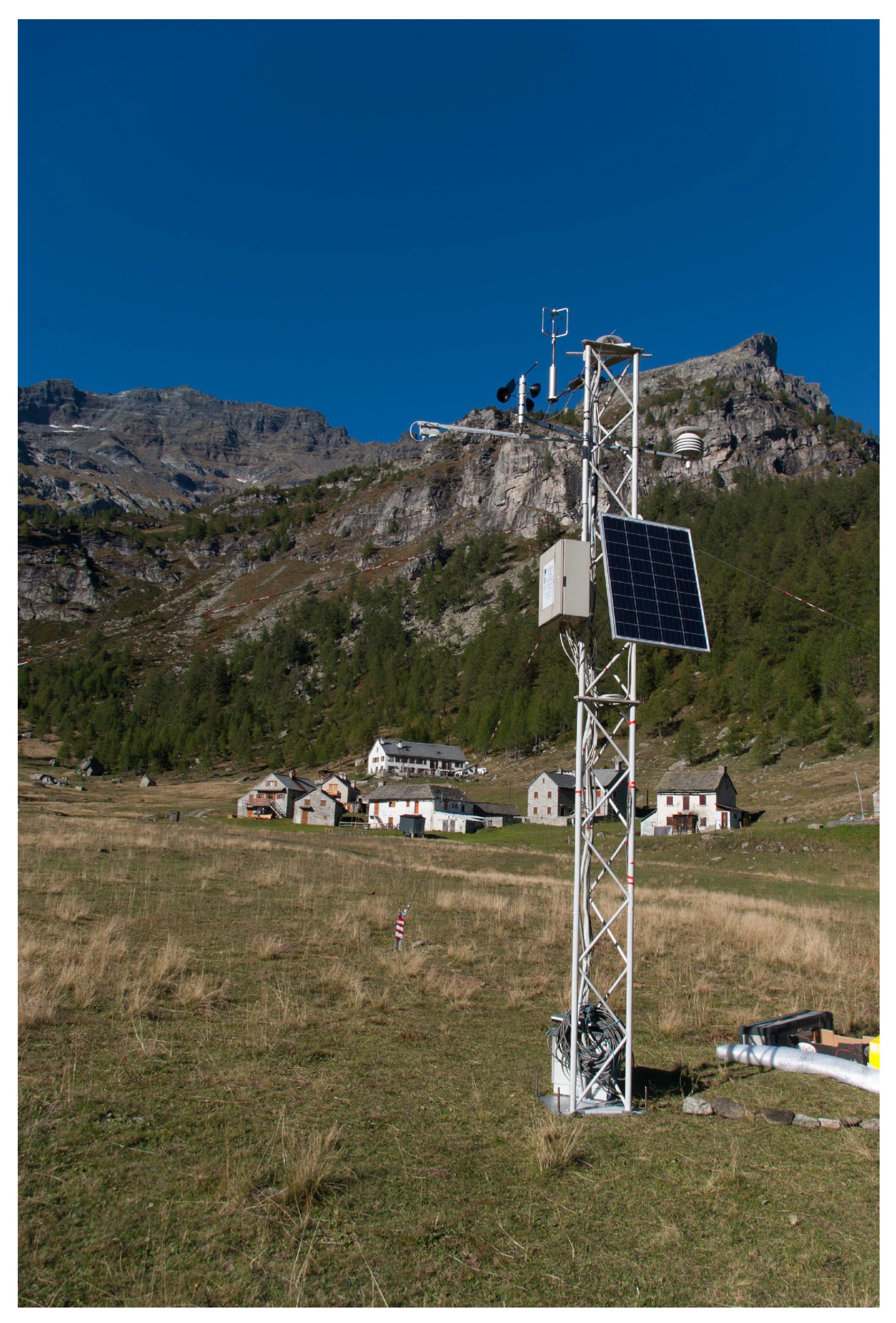
The station is equipped with standard meteorological instruments: a thermometer, wind vane, cup anemometer, barometer, radiometer and snow-meter. A sonic anemometer was installed with a couple of inclinometers for the measurement of turbulence. A complete description of the instrumentation is given in

Table 1. Description and positioning of the Alpe Veglia Station instrumentation.

Instrument	Make and Model	Ground and Mast Distance (±0.01 m)	Range	N Direction of the Instrument
Ultrasonic anemometer	Gill, Solent R2-research	$4.93$; $0.53$	±30 ms${}^{-1}$ 290 ms${}^{-1}$ to 370 ms${}^{-1}$	$8^{\circ }\pm 2^{\circ }$
Anemometer and wind vane	Siap+Micros, SVDV	$4.30$; $0.54$	0 ms${}^{-1}$ to 60 ms${}^{-1}$ 0${}^{\circ }$ to 359${}^{\circ }$	$8^{\circ }\pm 2^{\circ }$
Thermometer	Thermocouple type K	$4.28$; $0.43$	−200 ${}^{\circ }\mathrm{C}$ to 1260 ${}^{\circ }\mathrm{C}$
Snow-meter	HC-SR04	$4.17$; $1.05$	0 $\mathrm{m}$ to 5 $\mathrm{m}$
Radiometer	Eppley, PSP	$5.00$; $0.00$	0 Wm${}^{-2}$ to 2000 Wm${}^{-2}$
Barometer	Siap, TBAR	$3.20$; $0.00$	700 $\mathrm{hPa}$ to 1100 $\mathrm{hPa}$
Inclinometers	HLPlanar Technik, NS-5/PI	$4.93$; $0.45$	$\pm 5^{\circ }$	${337}^{\circ }\pm 2^{\circ }$

, and a comprehensive picture of the station mast is reported in Figure 2. The instruments were mounted relatively far from the ground because the snow in winter can reach a depth of 3 m.

2.2. Methods

2.2.1. Ultrasonic Anemometer Data Processing

The procedure applied to analyse the data has been used by many authors (including [19,21]). In the present case, the authors have adapted and re-elaborated the procedure according to the available dataset. It was applied to moving temporal windows of 30 or 60 min, moved forward by 15 min. The procedure consists of eight steps:

• Control of the instrumental electronic range, applying the following thresholds: ±30 ms${}^{-1}$ for the three components of the wind velocities u, v, w; 290 ms${}^{-1}$ to 370 ms${}^{-1}$ for the speed of sound c; 700 $\mathrm{hPa}$ to 1100 $\mathrm{hPa}$ for atmospheric pressure p.
• First, the despiking step over u, v, w, c, using an algorithm that replaces single spikes with the previous non-spike value. The block average and standard deviation ($\sigma$) were used in the despike algorithm, and spikes were defined as a point at a distance of more than $n\sigma$ from the window average. Here, we fixed $n=5$. Bursts were then removed using a linear regression of the neighbouring points. A burst is a step in instantaneous data that is higher than a fixed threshold (here $0.25\sigma$) with respect to the previous point. It should not exceed a number of consecutive points (four in this work) because, in this case, the data could represent physical behaviour of the eddies.
• Correction of the speed of sound. A previous calibration [22] was used.
• Calculation of sonic temperature $T_s$ from the speed of sound c with Equation (1)

  $$T_s=\frac{c^2}{\gamma R_d(1+0.502q)},$$

  (1)

  where $\gamma =1.4$, $R_d=287.05\mathrm{J}\mathrm{mol}{}^{-1}\mathrm{K}{}^{-1}$ is the gas constant for dry air and q is the specific humidity. If the specific humidity was not measured directly by a fast hygrometer or by a standard hygrometer via relative humidity, the denominator parenthesis in Equation (1) reduced to 1.
• Control of the extreme values of $T_s$ using Equation (2)

  $$|T_s-\overline{T_s}|<20\mathrm{K}.$$

  (2)
  Whenever a value fell outside this range, the entire instantaneous measurement record was nullified (u, v, w, $T_s$).
• Second despiking step with a $3\sigma$ threshold over u, v, w and $T_s$; burst control was not applied in this phase.
• Coordinate rotation calculation; all the data were moved from the anemometer reference system to a streamline reference system, according to the three rotation methods: Double Rotation (DR), Triple Rotation (TR) or Planar Fit (PF). The applied methods rotate the coordinate system, as explained in [9,10,11,12,14,23,24] and in the following Section 2.2.2.
• Final control of the valid physical range of the vertical wind speed $\left|w\right|$ < 5 ms${}^{-1}$. In this case, the w range is more restrictive than step 1.

After these eight steps, the covariances, variances, standard deviations and statistics were computed and saved in output files.

2.2.2. Coordinate Rotation Methods

The coordinate rotation methods are well explained in many textbooks (e.g., [14,24]). The first reference works are by Tanner and Thurtell (1969) [9] and Hyson et al. (1977) [23]. The aim of coordinate rotation is to provide a reference system on which the mean vertical velocity is negligible, otherwise the Eddy-Covariance method could not be used.

In the present field campaign, a couple of inclinometers have also been installed; they are very useful to correct the small inclination variations of the mast due to the elongation of steal stay that fastened it to the ground. This first correction is deeply described in Appendix A of Richiardone et al. (2008) [12], and essentially the anemometer reference system is placed, using the inclinometer angles, into a geographical horizontal reference system.

The first rotation turns the coordinate system around the z-axis, and place the x-axis into the direction of the mean wind. Expressing the notations similarly to Foken (2016) [14], the first rotation angle is

$$\theta =arctan\left(\frac{\overline{v_m}}{\overline{u_m}}\right).$$

(3)

The subscript m indicates the measured velocities, previously corrected with the inclinometers, and the overline indicates the temporal average (30 or 60 min in the present work). The new velocity components are:

$$\begin{array}{ccc}\hfill u_1& =& u_{m}cos\theta +v_{m}sin\theta ,\hfill \\ \hfill v_1& =& -u_{m}sin\theta +v_{m}cos\theta ,\hfill \\ \hfill w_1& =& w_m.\hfill \end{array}$$

(4)

The second rotation is around the new y-axis and it nullifies the mean vertical wind speed [25]. The second rotation angle is:

$$\psi =arctan\left(\frac{\overline{w_1}}{\overline{u_1}}\right)$$

(5)

and the new wind speeds could be expressed with:

$$\begin{array}{ccc}\hfill u_2& =& u_{1}cos\psi +w_{1}sin\psi ,\hfill \\ \hfill v_2& =& v_1,\hfill \\ \hfill w_2& =& -u_{1}sin\psi +w_{1}cos\psi .\hfill \end{array}$$

(6)

Applying this two rotation angles, $\theta$ and $\psi$, it is possible to identify the streamline flow; this is the Double Rotation method.

Furthermore, the last and third rotation is around the new x-axis, and as proposed by McMillen [10], it eliminates the covariance from the vertical and horizontal, normal to the mean wind direction, wind component. The rotation angle is:

$$\varphi =arctan\left(\frac{\overline{v_2{w}_2}}{\overline{v_2^2}-\overline{w_2^2}}\right).$$

(7)

The new wind speeds are:

$$\begin{array}{ccc}\hfill u_3& =& u_2,\hfill \\ \hfill v_3& =& v_{2}cos\varphi +w_{2}sin\varphi ,\hfill \\ \hfill w_3& =& -v_{2}sin\varphi +w_{2}cos\varphi .\hfill \end{array}$$

(8)

Applying all the three rotation angles means using the Triple Rotation method.

A different method to rotate into the mean stream line was proposed by Paw et al. (2000) [26] and Wilczak et al. (2001) [11]; it is the Planar Fit method. The main hypothesis of the PF method is that the flow lay on a plane. Differently from the previous methods that align the anemometer reference system to the streamline flow every 30 or 60 min, it computes the mean streamline plane over days or weeks of measurements. Therefore, the mean vertical velocity should be nullified by the calculation of the reference plane. The presence of the inclinometers helps to prevent errors from the modification of the anemometer positioning during the measures. Afterwards, the anemometer reference system is placed on the computed plane and the x-axis points into the mean wind direction. To describe the PF, a matrix form is more suitable, and, following the notation of Wilczak et al. (2001) [11], the $\overrightarrow{u_p}$ is the vector of the PF rotated wind velocities, $\overrightarrow{u_m}$ is the vector of measured velocities, $\overrightarrow{c}$ is an offset vector and P is a transformation matrix:

$$\overrightarrow{u_p}=P(\overrightarrow{u_m}-\overrightarrow{c}).$$

(9)

More details on the matrices are given in [11,12,14].

As aforementioned, the coordinate rotations had been applied at step 7 of Section 2.2.1; afterwards, the flux computation and analysis is done (Section 2.2.3, Section 2.2.4 and Section 3.2.4).

2.2.3. Turbulent Flux Calculation

The Sensible Heat flux (SH) represents the loss, or gain, of energy at the surface as a result of heat transfer to, or from, the atmosphere. SH is considered positive when the surface loses heat, i.e., when the heat flux is directed from the surface into the atmosphere. SH was computed with:

$$\mathrm{SH}=\rho c_p\overline{\left(w^{\prime }{T}_s^{\prime }\right)},$$

(10)

where the quantities $w^{\prime }$ and $T_s^{\prime }$ are the fluctuations of the vertical wind speed and sonic temperature, with respect to their mean value in the temporal window ($\overline{w}$, $\overline{T_s}$). The mean air density $\rho$ was calculated from the measured atmospheric pressure

$$\rho =\frac{100·\overline{p}}{R_d\overline{Ts}},$$

(11)

where $\overline{p}$ is the mean atmospheric pressure evaluated over the temporal window.

If $\overline{p}$ is not available, a fixed value of pressure can be used. In this work, when the pressure was not measured, a fixed value of 832.0 $\mathrm{hPa}$ was used because it corresponded to the mean atmospheric pressure measured at Alpe Veglia during the 49 days of the campaign.

The momentum fluxes were calculated with Equations (12) and (13):

$$Flu{x}_{u^{\prime }}=-\rho \overline{\left(u^{\prime }{w}^{\prime }\right)},$$

(12)

$$Flu{x}_{v^{\prime }}=-\rho \overline{\left(v^{\prime }{w}^{\prime }\right)},$$

(13)

where $u^{\prime }$ and $v^{\prime }$ are the fluctuations of the u and v wind speeds, compared with their averaged values.

2.2.4. Flux Quality Control Assessment

The calculated heat and momentum flux values, like any others physical quantity, were affected by uncertainties, which propagated throughout the calculation. It is of crucial importance to know these uncertainties. In fact, the quality of momentum and sensible heat fluxes is assessed by means of statistical tests based on uncertainties. In the present work, the quality assessment of the fluxes was conducted after calculating the fluxes, according to three stages [19]:

• Physical range control of the SH flux;
• Skewness and kurtosis limit control;
• Uncertainty and stationarity control.

The first stage involved applying a filter on SH, whereby values outside the −300 Wm${}^{-2}$ to 800 Wm${}^{-2}$ range were deleted. Moreover, at least 95% of data are necessary for each window. A further control was applied to the sonic temperature, whose standard deviation in each window should be below the 99th quantile of the ${\sigma }_{Ts}$ probability distribution function. In the present work, ${\sigma }_{Ts}\left(99\mathrm{th}\right)=5.8\mathrm{K}$. The SH fluxes that did not satisfy the physical range controls were excluded from the dataset.

The second stage considered skewness (${\gamma }_1$) limits of −2 to 2, and an upper kurtosis (${\gamma }_2$) limit of 8 [27]. Skewness and kurtosis were calculated according to Equations (14) and (15), respectively:

$${\gamma }_1=\frac{m_3}{m_2^{3/2}},$$

(14)

$${\gamma }_2=\frac{m_4}{m_2^2}-3,$$

(15)

where:

$$m_n=\frac{1}{N}\sum _{i=1}^N{(x_i-\overline{x})}^n.$$

(16)

x is a generic variable (u, v, w, $T_s$) and N is the number of elements contained in the temporal window analysed for the x variable.

The third stage considered the uncertainty involved when determining the covariances or variances of turbulent variables. In fact, according to Wyngaard [20], it is well known that the time window used for covariance computation may not consider the full turbulence spectrum. Wyngaard [20] approached the problem directly, and stated that, in order to decrease uncertainties, it was necessary to modify the integrating time (window size). Stiperski and Rotach [19] approached the problem in a different way: the integrating time, ${\tau }_a$, is considered constant (e.g., 30 or 60 min) and the covariances uncertainty is therefore defined as:

$$a_{uw}^2=\frac{z}{{\tau }_a·U}\left[\frac{\overline{{\left(u^{\prime }{w}^{\prime }\right)}^2}}{u_{*}^4}-1\right],$$

(17)

$$a_{vw}^2=\frac{z}{{\tau }_a·U}\left[\frac{\overline{{\left(v^{\prime }{w}^{\prime }\right)}^2}}{u_{*}^4}-1\right],$$

(18)

$$a_{w{T}_s}^2=\frac{z}{{\tau }_a·U}\left[\frac{\overline{{\left(w^{\prime }{T}_s^{\prime }\right)}^2}}{{\left(\overline{w^{\prime }{T}_s^{\prime }}\right)}^2}-1\right],$$

(19)

where $U=\sqrt{{\overline{u}}^2+{\overline{v}}^2}$ is the mean horizontal wind value, $u_{*}=\sqrt[4]{{\overline{\left(u^{\prime }{w}^{\prime }\right)}}^2+{\overline{\left(v^{\prime }{w}^{\prime }\right)}}^2}$ is the friction velocity and z is the ultrasonic anemometer height. The limit imposed on a quantities is 0.5, according to [19]. By starting with Equations (17)–(19), it was possible to evaluate the variances (and standard deviations) of the turbulent fluxes:

$${\sigma }_{\overline{u^{\prime }{w}^{\prime }}}^2=a_{uw}^2·{\overline{u^{\prime }{w}^{\prime }}}^2,$$

(20)

$${\sigma }_{\overline{v^{\prime }{w}^{\prime }}}^2=a_{vw}^2·{\overline{v^{\prime }{w}^{\prime }}}^2,$$

(21)

$${\sigma }_{\mathrm{SH}}^2=a_{w{T}_s}^2·{\mathrm{SH}}^2.$$

(22)

The stationarity of each interval can be assessed using an a posteriori test. Several tests are available (among others: [27,28,29]), and, from a comparison made by Večenaj and De Wekker (2015) [30] and a previous work in complex terrain [19], it resulted that the test proposed by Foken and Wichura (1996) [28] was the most appropriate. The test (hereafter referred to as steady test) was evaluated using the following equation:

$$R{N}_{cov}=\left|\frac{-\overline{{\left(x^{\prime }{y}^{\prime }\right)}_{SI}}+\overline{{\left(x^{\prime }{y}^{\prime }\right)}_{WI}}}{\overline{{\left(x^{\prime }{y}^{\prime }\right)}_{WI}}}\right|·100,$$

(23)

where WI indicates the 30 or 60 min long windows, SI a sub-window of 5 min, while the generic x and y can be substituted with the $(u,w)$, $(v,w)$ or $(w,T_s)$ pairs. The threshold was here fixed at 40 (unlike its standard level of 30), to account for the major complexities of this high mountain site.

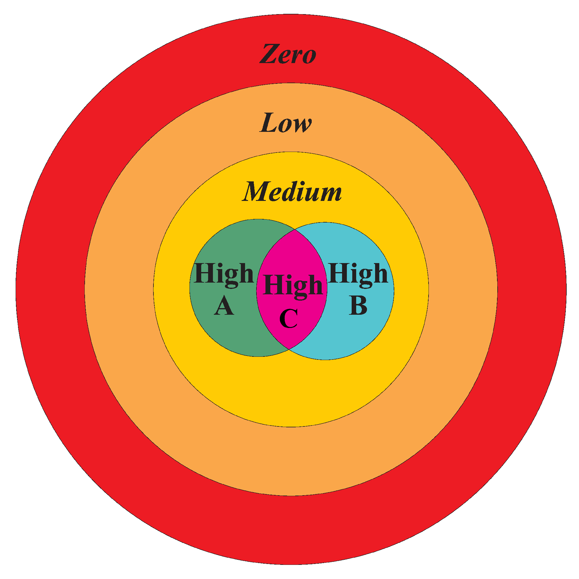
These three stages permit the quality of turbulence data to be classified. There are six quality levels, and they may be graphically represented with the nesting sets shown in Figure 3.

The initial level (zero) contains all the data that passed the previous eight control steps described in Section 2.2.1. The first stage control was then performed and the data that passed this control entered the low-quality level. The second quality control was than applied, then kurtosis and skewness were checked, and, if they fell within the allowed range, the data entered into the medium-quality level. The third quality controls were applied separately to medium-quality data. Data that showed lower a uncertainties than 0.5 entered the high A-quality level, while the data that were stationary ($R{N}_{cov}<40$, Equation (23)) entered the high B-quality level. The intersection of high A and high B that assumes the positivity of both the a uncertainty test and steady test is the high C-quality level.

3. Results

3.1. Overview of the Standard Meteorological Data

Data collected once per minute by standard meteorological instruments (Table 1) were considered, whereas the precipitation data were taken from the ARPA Piemonte (Environmental Protection Agency of the Piedmont Region) nivometric station, located 500 m from the mast, which measures the cumulated rain every ten minutes and the snow depth.

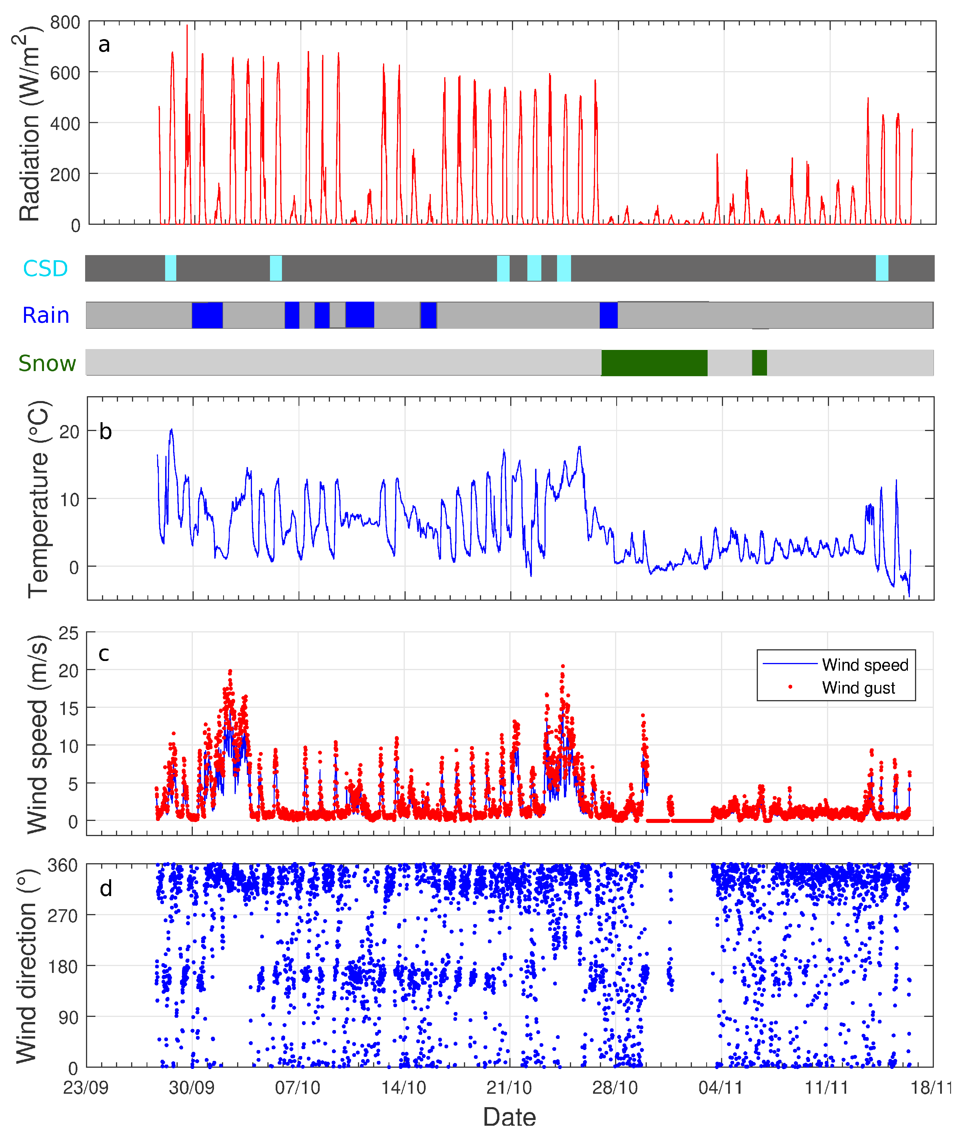
The complete analysed dataset consisted of 49 complete days. By first analysing the low frequency data, and in particular the radiometer data (Figure 4a), it emerged that only six days have a completely clear-sky (28 September; 5, 20, 22, 24 October; 14 November 2018). These days are depicted in the first timeline in Figure 4. The total precipitation for 49 days was 896 $\mathrm{m}\mathrm{m}$, and it was distributed over 16 days. The rainy days were: 30 September; 1, 6, 8, 10, 11, 15, 27 October (second timeline in Figure 4). It snowed between 28 October and 3 November, and the snow reached a depth of 113 $\mathrm{c}\mathrm{m}$. A second snowfall event affected Alpe Veglia on 6 November and the fresh snow was 10 $\mathrm{c}\mathrm{m}$ deep (third timeline in Figure 4). The snow depth and cumulated rain from 27 September is shown in Figure 5, where the snow depth below 20 $\mathrm{c}\mathrm{m}$ is not reliable.

Figure 4b reports the air temperature measured at the Alpe Veglia Station. Two main periods are recognisable in the temperature time series, the first from 27 September to 26 October, which was characterised by a mean daily temperature at about 6 ${}^{\circ }\mathrm{C}$ and a daily excursion of 10 ${}^{\circ }\mathrm{C}$; the second period was between 27 October and 12 November, and it was characterised by a daily temperature of 2.5 ${}^{\circ }\mathrm{C}$ and a daily excursion of 4–5 ${}^{\circ }\mathrm{C}$. Snowfall occurred at Alpe Veglia at the beginning of the second period (Figure 5) and the snow layer contributed to reducing the air temperature.

The wind regime was characterised by daily cycles with different amplitudes over the two periods (Figure 4c,d), the second period was in fact marked by low wind values, linked to the presence of cloudy days and snow on the ground (from 4 to 13 November 2018). By analysing the wind vane and cup anemometer, it was possible to generate a comprehensive wind rose (Figure 6). The timeseries data showed that the anemometer was probably blocked by snow and ice between 30 October and 2 November (Figure 4c,d). The wind rose denoted that the main wind direction was from NNW and SSE. This direction corresponds to the main axis of the Alpe Veglia plain, which is oriented from the south-facing slope near the Italian–Swiss border and the southern border of Alpe Veglia, where the entrance to the plain is located.

The most intense winds came from the northern side, and they may have been related to the Föhn or strong down-slope winds from the North.

3.2. Ultrasonic Anemometer Data Analysis

The ultrasonic instrument collected data during the 49-day campaign with a frequency of 10 $\mathrm{Hz}$. The data were analysed using moving windows of 30 and 60 min time length windows. A total of 4777 temporal windows were available and 4644 (30 min integration interval) and 4657 (60 min integration interval) were actually analysed (windows that had passed the eight-step procedure in Section 2.2.1), which corresponded to $97.22\%$ and $97.49\%$, respectively. The turbulent fluxes (Equations (10), (12) and (13)) were computed using the DR, TR and PF methods for these subsets. The SH flux during clear-sky days (Figure 7) showed a typical daily cycle, with approximately 150 Wm${}^{-2}$ at noon and −50 Wm${}^{-2}$ during the night (the upward fluxes were positive). The quality assessment (Section 2.2.4) was performed on the same subsets of the entire dataset.

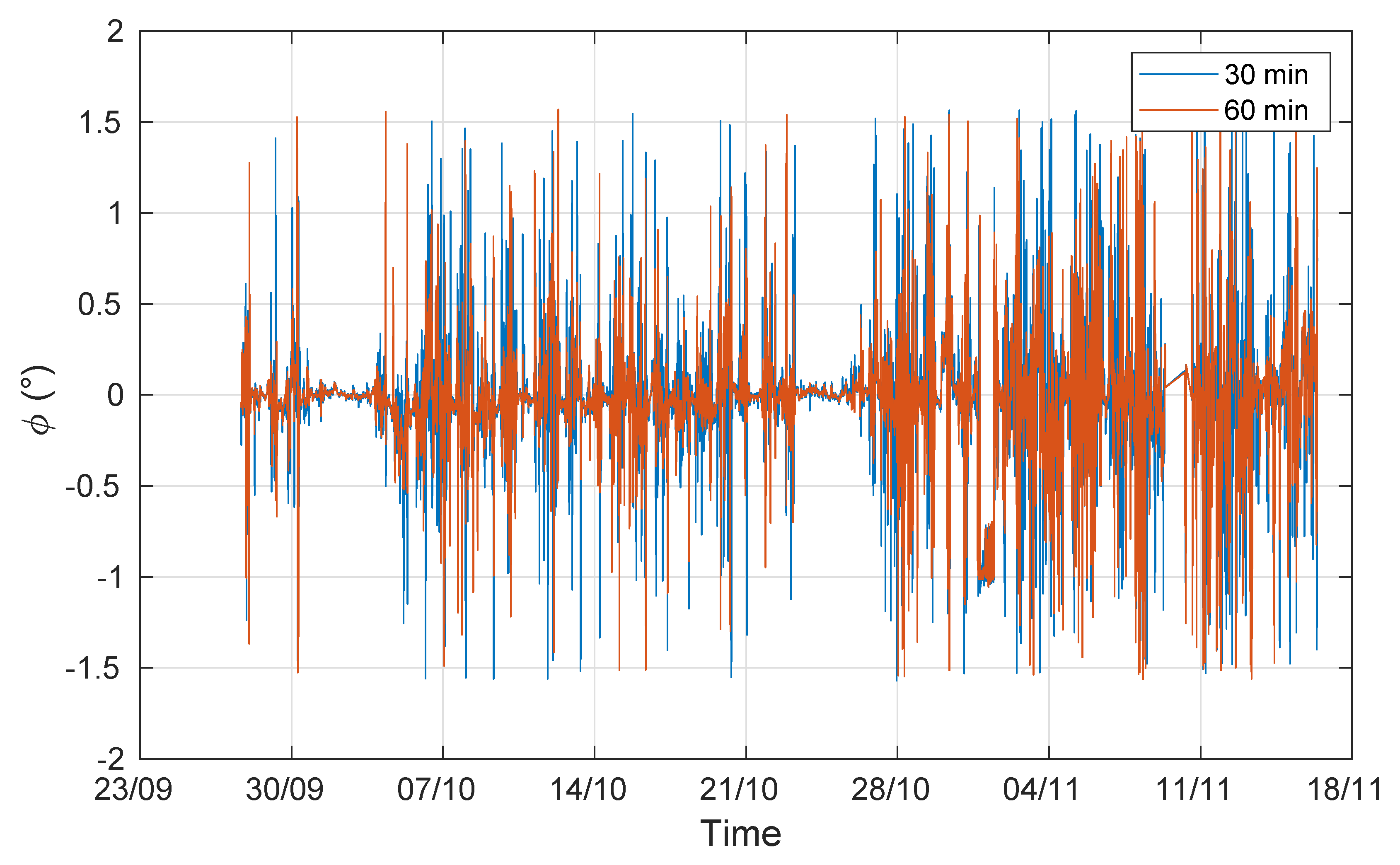
It is important to highlight that the reliability of ultrasonic anemometer measurements during rain or snow events is very low. Falling snowflakes and raindrops between the transducers in fact compromise the measurements. The weather conditions during the experiment are described briefly in Section 3.1. It is possible to see, in Figure 5, the time-series of ${\sigma }_{\mathrm{SH}}$ (Equation (22)) along with the cumulated rain and the snow depth. High standard deviations were obtained during rainfall and snowfall, and this could be responsible for the poor reliability of the ultrasonic anemometer measurements during these periods. In fact, the two periods of fine and cloudy weather conditions that were identified in the temperature, short-wave incoming radiation and wind speed measurements were also captured in the SH standard deviation time series.

The data quality of the heat and momentum fluxes was dealt with here according to the procedure outlined in Section 2.2.4. The overall data quality showed that the most populated class was high A (

Table 2. Data quality for the Alpe Veglia ultrasonic anemometer dataset. The quality levels are described in Section 2.2.4. The low data passed the first control; medium data passed the first and second controls; high A data passed the first, second and uncertainty controls; high B data passed the first, second and steady test controls; the high C data passed all the controls. No $Flu{x}_{v^{\prime }}$ statistics were evaluable for the TR definition.

Variable	Quality Level	DR		TR		PF
		30 min	60 min	30 min	60 min	30 min	60 min
$SH$	zero	8.46%	4.98%	7.99%	4.64%	10.96%	6.87%
	low	0.04%	0.11%	0.04%	0.11%	0.04%	0.15%
	medium	30.32%	38.29%	35.47%	46.03%	31.37%	39.68%
	high A	61.18%	56.58%	56.46%	52.18%	57.62%	53.25%
	high B	0.00%	0.04%	0.04%	0.04%	0.00%	0.04%
	high C	0.00%	0.00%	0.00%	0.00%	0.00%	0.00%
$Flu{x}_{u^{\prime }}$	zero	0.00%	0.00%	0.00%	0.00%	0.00%	0.00%
	low	0.04%	0.04%	0.09%	0.04%	0.04%	0.09%
	medium	4.93%	5.18%	15.87%	14.54%	1.85%	1.87%
	high A	94.90%	94.67%	83.91%	85.27%	97.83%	97.90%
	high B	0.02%	0.02%	0.11%	0.15%	0.00%	0.00%
	high C	0.11%	0.09%	0.02%	0.00%	0.28%	0.25%
$Flu{x}_{v^{\prime }}$	zero	0.00%	0.00%			0.00%	0.00%
	low	0.02%	0.02%			0.04%	0.09%
	medium	4.69%	4.60%			1.21%	1.10%
	high A	95.09%	95.28%			98.62%	98.80%
	high B	0.00%	0.00%			0.00%	0.00%
	high C	0.19%	0.11%			0.13%	0.02%

), that is, data that had passed the first two steps in Section 2.2.4 and had an uncertainty $a<0.5$. The momentum fluxes showed a higher quality than the sensible heat flux, probably as a consequence of how the fluxes had been defined; the momentum fluxes were directly computed from measured quantities (u, v, w), whereas SH was computed from a derived quantity ($T_s$).

The data quality results and a comparison of the SH standard deviations are presented in the following subsections.

3.2.1. Double Rotation

Table 2 reports the results of the quality classification of the momentum and sensible heat fluxes as percentages. The high C-quality class was only filled for the momentum fluxes and higher values considering the 30 min windows. By observing the high B quality data, it is clear that the steady test was the most difficult to pass, and low uncertainties were frequently present (high A class).

3.2.2. Triple Rotation

Triple rotation may be applied if, as suggested by McMillen [10], the third rotation angle $\varphi$ is lower than 10°, otherwise, especially in low wind speed conditions, the third angle could enhance the uncertainty of turbulent quantities. The distribution of $\varphi$ and its time evolution are depicted in Figure 8 and Figure 9; the $\varphi$ values were always lower than ten degrees over a range of −2${}^{\circ }$ to 2${}^{\circ }$, and the largest variations were only found for low wind speed conditions (Figure 4c and Figure 9). As a consequence, the TR rotation produced different results from the DR rotation, albeit only under low wind conditions (notwithstanding the limit at $\left|\varphi \right|<{10}^{\circ }$).

The quality statistics of the fluxes are reported in Table 2. Unlike the double rotated data, fewer values fell into the “high A” class, for both the heat and momentum fluxes. This suggests higher uncertainties with respect to DR.

3.2.3. Planar Fit

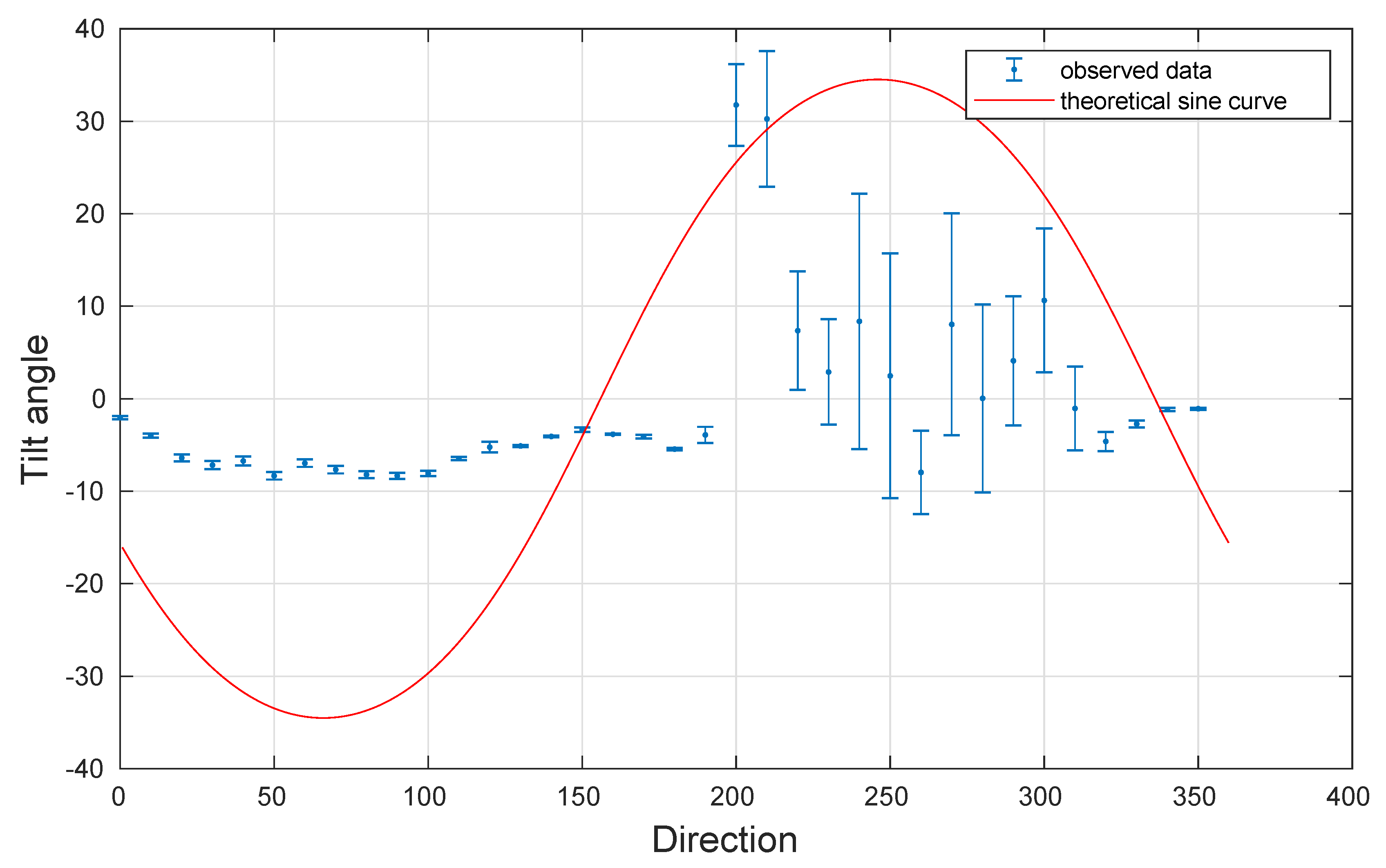
The planar fit parameters were evaluated on 5 min averages of the wind speed components, using all the 49-day data. The planar fit plane was determined by computing the azimuth of orientation $\omega$ (clockwise from the North) of the PF plane and tilt $\nu$ above the horizontal plane. Tilt angle $\nu =34.5$° was quite large as a result of the slope of the terrain, and its uncertainty (of about $0.2$°) was also quite large, compared to the same quantity obtained from experiments on flat terrain [12], where its value was one order of magnitude lower.

In order to verify the reliability of the obtained PF plane, it is possible to plot the computed plane and the mean wind value for each sector. If the data lie on the computed plane, the method is relevant. Considering the results in Figure 10, where a single PF plane (red line) was not able to interpolate the wind vectors, it is possible to observe that the Alpe Veglia data do not show a precise plane. This may be explained considering the wind distribution (Figure 6), which showed two opposite preferential directions. The wind vectors at Alpe Veglia seem to depict the presence of two overlapping planes as a consequence of a three-dimensional streamline surface. In this case, it could be useful to apply the directional planar fit, as suggested by Nadeau et al. (2012) [31].

A quality control on the PF data indicated (Table 2) that there were more “zero” quality SH data than for the DR and TR methods, while class “high A” was as heavily populated as the TR “high A” class. The momentum fluxes show that more than 97% of the data had low uncertainties, but they did not pass the steady test, and a rather small part, but comparable with DR, was in the “high C” class.

In conclusion, the flow was not planar and the PF method was not applicable, but the PF method uncertainties were low. These results suggest that caution is needed in judging a method using data quality only.

3.2.4. Comparison of the Sensible Heat Flux Standard Deviations

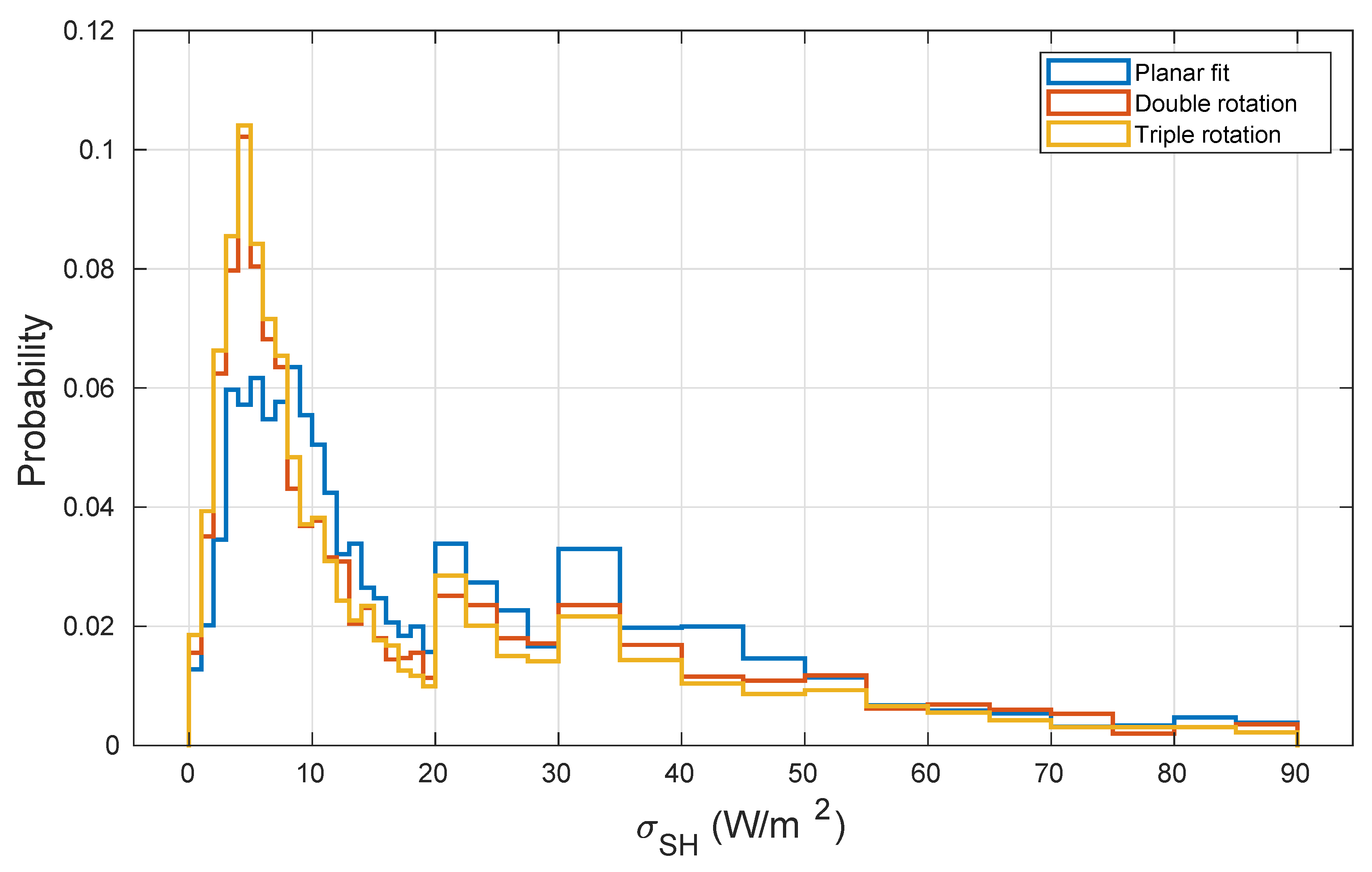
Further considerations may be made taking into account only the standard deviations of the sensible heat flux, which were evaluated with the Stiperski and Rotach method [19] (see Equation (22)). The aim was to compare the three different coordinate rotation methods considering all the data that were at a minimum at the low quality level (zero quality-level data were excluded). The ${\sigma }_{\mathrm{SH}}$ values were plotted in bins of 1 Wm${}^{-2}$ from 0 Wm${}^{-2}$ to 20 Wm${}^{-2}$, of 2.5 Wm${}^{-2}$ from 20 Wm${}^{-2}$ to 30 Wm${}^{-2}$ and of 5 Wm${}^{-2}$ from 30 Wm${}^{-2}$ to 90 Wm${}^{-2}$ (Figure 11 and Figure 12). The distribution peaks of the 30 and 60 min windows are very similar, and are at about 5 Wm${}^{-2}$ for the DR and TR values. The slightly higher score of TR than of DR is appreciable in Figure 11 and Figure 12, where it may also be noted that the standard deviations of the TR and DR heat fluxes have lower values than the PF ones. In fact, $29.5\%$ of the DR data, $31.4\%$ of the TR data and $18.4\%$ of the PF data are below 5 Wm${}^{-2}$ for the 30 min window. The distribution for the 60 min window is: $19.8\%$ for the DR data, $21.3\%$ for the TR data and only $11.3\%$ for the PF data. As a consequence, longer windows did not generally produce smaller standard devations. In fact, there is a drop of 10% in the analysis conducted with the 60 min windows compared to that conducted with 30 min windows below the 5 Wm${}^{-2}$ limit. In other words, there are fewer data with a standard deviation below 5 Wm${}^{-2}$ in the case of the 60 min windows.

4. Discussion

The analysed period presents a first part that is characterised by warm and relatively good weather (27 September–26 October) and a second part characterised by rain, snow and cloudy weather (27 October–13 November). This influences the quality of the ultrasonic anemometer data and also the values of ${\sigma }_{\mathrm{SH}}$.

From the low frequency data, it was possible to extract the mean wind conditions for the full 49-day dataset. It was found that Alpe Veglia is characterised by two main wind directions. The first is related to northerly more intense winds (NNW), while the second pertains to southerly “in-plain” winds (SSE).

A filtering procedure was applied to the high frequency data and the turbulent fluxes were computed according to the DR, TR and PF coordinate rotation methods. It has emerged from the analysis that the DR and TR results are significantly different from each other, albeit only for the low-wind conditions that were experienced most of the time at Alpe Veglia (but $\left|\varphi \right|<2$°), when the streamline plane was not clearly defined and, consequently, showed higher a parameter values than DR. However, in high-wind conditions, the $\varphi$ third rotation angle was zero and TR reproduced the same results as DR. PF was not able to identify a reliable plane (Figure 10), and this could be related to a lack of wind from the Eastern and Western sectors, which destabilises the plane, or even to the flow assumed to have a multi-planar form, due to the complexity of the sloped orography at Alpe Veglia; in this sense, the directional planar fit method could improve the analysis [31].

The quality control of the SH flux revealed a slightly better performance for the TR data, which had more populated “medium” and “high” quality classes than the DR data of 0.5% and than the PF data of 3%, but the “high-A” quality class of the DR data reached higher values than the TR data. The momentum flux percentage showed a higher quality for the DR method than for the TR one. However, the Alpe Veglia dataset had only a few half-hour or one hour periods of “high C”-quality data, and the flow stationarity was not usually fulfilled, probably due to the complex surrounding terrain. Finally, the standard deviation distribution of SH was comparable for the DR and TR data, with slightly better values for TR as consequence of the lower SH values during the second period and at night, and during the twilight and dawn hours in the first period.

Two integration lengths were used in the present work. The basic idea was that longer windows should include a greater part of the turbulent spectrum, e.g., more powerful eddies. However, from Table 2 and from Section 3.2.4, it emerges that longer windows did not produce smaller standard deviations for the sensible heat flux. A smaller decrease in the percentage of the heat flux standard deviation of the heat fluxes than 5 Wm${}^{-2}$, that is, of about 10%, was in fact observed.

The aforementioned results could be partially compared with similar experiments that had been conducted in complex terrains. However, the complexity of the sites hereafter presented may not be completely the same. A similar comparison work were done by Yuan et al. (2007) [32] at a hilly forest catchment. They compared DR, TR and PF, but the final conclusions dealt only with DR and PF, and they stated that DR and PF were comparable, but with better perfomances of the latter regarding the friction velocity. A comprehensive comparison between different coordinate rotation methods were done by Shimizu (2015) [33]. He considered seven different rotation methods, but he compared them against the DR; in other words, he considered the DR as the standard rotation method. Among all of them, the PF resulted as the most interesting, while the directional PF underestimated nocturnal heat fluxes. From the statistical analysis, the best one was the method proposed by Lee [34]. Another comparison study was done at the Ameriflux site of Niwot Ridge [35]. Turnipseed et al. [35] obtained small rotation angles, similarly to the Alpe Veglia site, for every rotation method and assessed the equality of DR, TR and PF. The iBox-project is noteworthy, and, in particular, the Stiperski and Rotach (2016) [19] paper that considered only DR, PF and directional PF; the best performances were obtained with the DR method. This work is more comparable for the similar quality assessment procedure, and it is noteworthy that, as pointed out by the authors Stiperski and Rotach, the most difficult achievement is $a<0.5$ and not the steady test. In the Alpe Veglia site and also in an unpublished MSc Thesis [36] done on Arbeser Kogel iBox station data, it was the opposite because it resulted that the steady test was the hardest to accomplish. This difference of results, among the valley stations of the iBox, the mountain top station of the iBox (Arbeser Kogel) and the Alpe Veglia station could be found in the major complexities present in the last two sites that, from this point of view, could be more comparable.

5. Conclusions

Some key points can be summarised from the results obtained in the Alpe Veglia campaign:

• The PF method was hard to apply in Alpe Veglia complex terrain because the flow was not planar; instead, the wind flow was on a three-dimensional surface. As suggested by Nadeau et al. [31], it could be useful to apply the directional planar fit.
• The TR method has a much smaller third rotation angle $\varphi$ than the threshold suggested by McMillen [10]. This suggests that the TR method could be useful, especially for low wind cases that were mostly experienced at the Alpe Veglia site.
• Two different procedures have been applied to define the trustworthiness of SH flux calculated by the three coordinate rotation methods: the quality control procedure (Section 2.2.4) and the SH standard deviation (Section 3.2.4). Considering the high-quality class, the DR method obtained the best results in the 30 and 60 min integration interval ($61.18\%$ and $56.58\%$ Table 2), whereas, considering the merged classes medium and high, the best result is for the TR method ($91.93\%$ and $98.21\%$). Considering the standard deviation on SH, and a threshold of 5 Wm${}^{-2}$, the best result is given by the TR method, while PF performs the worst. The biggest difference between the two methods arose in the PF, which obtained a high rating with the quality assessment, but very high standard deviations were computed; this reflects the senselessness of the detected PF-plane.
• The stationarity test (or steady-test) is harder to obtain at Alpe Veglia, and this could be linked to the applied test or to the constitution of the turbulence in the Alpe Veglia location.

The results offer a description of the conditions in such a complex site, and the ongoing campaign at Alpe Veglia will surely reveal more information on interactions between high mountain territories. A correct computation of turbulent fluxes is interesting for the studies of interactions between MBL and areas with pastures and woods in a changing environment. The measurements and physical understanding of fluxes in a nival or glacial/paraglacial environment could offer valuable tools for the interpretation of the weather acting on different ecosystem components in such fragile and fast-changing landscapes.

References

- Bollati, I.; Reynard, E.; Lupia Palmieri, E.; Pelfini, M. Runoff impact on Active Geomorphosites in uncosolidated substrate. A comparison between landforms in glacial and marine clay sediments: Two case studies from the Swiss Alps and the Italian Appennines. Geoheritage 2016, 8, 61–75. [Google Scholar] [CrossRef]
- D’Agata, C.; Diolaiuti, G.; Maragno, D.; Smiraglia, C.; Pelfini, M. Climate change effects on landscape and environment in glacierized Alpine areas: Retreating glaciers and enlarging forelands in the Bernina group (Italy) in the period 1954–2007. Geol. Ecol. Landsc. 2019. [Google Scholar] [CrossRef]
- Bollati, I.; Pellegrini, M.; Reynard, E.; Pelfini, M. Water driven processes and landforms evolution rates in mountain geomorphosites: Examples from Swiss Alps. Catena 2017, 158, 321–339. [Google Scholar] [CrossRef]
- Pelfini, M.; Diolaiuti, G.; Leonelli, F.; Bozzoni, M.; Bressan, N.; Brioschi, D.; Riccardi, A. The influence of glacier surface processes on the short-term evolution of supraglacial tree vegetation: The case study of the Miage Glacier, Italian Alps. Holocene 2012, 8, 847–857. [Google Scholar] [CrossRef]
- Eichel, J. Vegetation succession and biogeomorphic interactions in glacier forelands. In Geomorphology of Proglacial Systems; Springer: Berlin/Heidelberg, Germany, 2019; pp. 327–349. [Google Scholar]
- Lehner, M.; Rotach, M.W. Current challenges in understanding and predicting transport and exchange in the atmosphere over mountainous terrain. Atmosphere 2018, 9, 276. [Google Scholar] [CrossRef]
- Rotach, M.W.; Gohm, A.; Leukauf, D.; Stiperski, I.; Wagner, J.S. On the vertical exchange of heat, mass, and momentum over complex, mountainous terrain. Front. Earth Sci. 2015, 3, 1–14. [Google Scholar] [CrossRef]
- Finnigan, J.J. A re-evaluation of long-term flux measurement techniques—Part II: Coordinate systems. Bound. Layer Meteorol. 2004, 113, 1–41. [Google Scholar] [CrossRef]
- Tanner, C.B.; Thurtell, G.W. Anemoclinometer Measurements of Reynolds Stress and Heat Transport in the Atmospheric Surface Layer; ECOM, United States Army Electronics Command, Research and Development: Aberdeen, MD, USA, 1969.
- McMillen, R.T. An eddy correlation technique with extended applicability to non-simple terrain. Bound. Layer Meteorol. 1988, 43, 231–245. [Google Scholar] [CrossRef]
- Wilczak, J.M.; Oncley, S.P.; Stage, S.A. Sonic anemometer tilt correction algorithms. Bound. Layer Meteorol. 2001, 99, 127–150. [Google Scholar] [CrossRef]
- Richiardone, R.; Giampiccolo, R.; Ferrarese, S.; Manfrin, M. Detection of flow distortion and systematic errors in sonic anemometry using the planar fit method. Bound. Layer Meteorol. 2008, 128, 277–302. [Google Scholar] [CrossRef]
- Stull, R.B. An Introduction to Boundary Layer Meteorology; Kluwer Academic Publishing: Norwell, MA, USA, 1988. [Google Scholar]
- Foken, T. Micrometeorology, 2nd ed.; Springer: Berlin/Heidelberg, Germany, 2016. [Google Scholar]
- Francone, C.; Cassardo, C.; Spanna, F.; Alemanno, L.; Bertoni, D.; Richiardone, R.; Vercellino, I. Preliminary results on the evaluation of factors influencing evatranspiration processes in vineyards. Water 2010, 2, 916–937. [Google Scholar] [CrossRef]
- Trini Castelli, S.; Falabino, S.; Mortarini, L.; Ferrero, E.; Richiardone, R.; Anfossi, D. Experimental investigation of surface-layer parameters in low wind-speed conditions in a suburban area. Q. J. R. Meteorol. Soc. 2014, 140, 2023–2036. [Google Scholar] [CrossRef]
- Rotach, M.W.; Stiperski, I.; Fuhrer, O.; Goger, B.; Gohm, A.; Obleitner, F.; Rau, G.; Sfyri, E.; Vergeiner, J. Investigating Exchange Processes over Complex Topography: The Innsbruck–Box (i-Box). Bull. Am. Meteorol. Soc. 2017. [Google Scholar] [CrossRef]
- Rigamonti, I.; Uggeri, A. L’evoluzione dell’Alpe Veglia nel quadro delle Alpe Centrali. Geol. Insubrica 2016, 1, 69–83. [Google Scholar]
- Stiperski, I.; Rotach, M.W. On the measurements of turbulance over complex mountainous terrain. Bound. Layer Meteorol. 2016, 159, 97–121. [Google Scholar] [CrossRef]
- Wyngaard, J.C. Workshop on micrometeorology. In On Surface–Layer Turbulence; American Meteorological Society: Boston, MA, USA, 1973; pp. 101–149. [Google Scholar]
- Rebmann, C.; Kolle, O.; Heinesch, B.; Queck, R.; Ibrom, A.; Aubinet, M. Data Acquisition and Flux Calculations. In Eddy Covariance; Springer: Berlin/Heidelberg, Germany, 2012; pp. 59–84. [Google Scholar]
- Richiardone, R.; Manfrin, M.; Ferrarese, S.; Francone, C.; Fernicola, V.; Gavioso, R.; Mortarini, L. Influence of the sonic anemometer temperature calibration on turbulent heat-flux measurements. Bound. Layer Meteorol. 2012, 142, 425–442. [Google Scholar] [CrossRef]
- Hyson, P.; Garratt, J.R.; Francey, R.J. Algebraic and electronic corrections of measured uw covariance in the lower atmosphere. J. Appl. Meteorol. 1977, 16, 43–47. [Google Scholar] [CrossRef]
- Aubinet, M.; Vesala, T.; Papale, D. Eddy Covariance: A Practical Guide to Measurement and Data Analysis; Springer: Berlin/Heidelberg, Germany, 2012. [Google Scholar]
- Kaimal, J.C.; Finnigan, J.J. Atmospheric Boundary Layer Flows: Their Structure and Measurements; Oxford University Press: Oxford, UK, 1994. [Google Scholar]
- Paw, U.K.T.; Baldocchi, D.; Meyers, T.P.; Wilson, K.B. Correction of eddy covariance measurements incorporating both advective effects and density fluxes. Bound. Layer Meteorol. 2000, 97, 487–511. [Google Scholar] [CrossRef]
- Vickers, D.; Mahrt, L. Quality control and flux sampling problems for tower and aircraft data. J. Atmos. Ocean Technol. 1997, 14, 512–526. [Google Scholar] [CrossRef]
- Foken, T.; Wichura, B. Tools for quality assessment of surface-based flux measurements. Agric. For. Meteorol. 1996, 78, 83–105. [Google Scholar] [CrossRef]
- Mahrt, L. Flux sampling errors for aircraft and towers. J. Atmos. Ocean. Technol. 1998, 15, 416–429. [Google Scholar] [CrossRef]
- Večenaj, Z.; De Wekker, S.F.J. Determination of non-stationarity in the surface layer during the T-REX experiment. Q. J. R. Meteorol. Soc. 2015, 141, 1560–1571. [Google Scholar] [CrossRef]
- Nadeau, D.F.; Pardyjak, E.R.; Higgins, C.W.; Huwald, H.; Parlange, M.B. Flow during the evening transition over steep Alpine slopes. Q. J. R. Meteorol. Soc. 2012, 139, 607–624. [Google Scholar] [CrossRef]
- Yuan, R.; Minseok, K.; Sungbin, P.; Jinkyu, H.; Dongho, L.; Joon, K. The effect of coordinate rotation on the eddy covariance flux estimation in a hilly KoFlux forest catchment. Korean J. Agric. For. Meteorol. 2007, 9, 100–108. [Google Scholar] [CrossRef]
- Shimizu, T. Eeffects coordinate rotation systems on calculated fluxes over a forest in complex terrain: A comprehensive comparison. Bound. Layer Meteorol. 2015, 156, 277–301. [Google Scholar] [CrossRef]
- Lee, X. On micrometeorological observation of surface-air exchange over tall vegetation. Agric. For. Meteorol. 1998, 91, 29–49. [Google Scholar] [CrossRef]
- Turnipseed, A.A.; Anderson, D.E.; Blanken, P.D.; Baugh, W.M.; Monson, R.K. Airflows and turbulent flux measurements in mountainous terrain Part 1. Canopy and local effects. Agric. For. Meteorol. 2003, 119, 1–21. [Google Scholar] [CrossRef]
- Golzio, A. Near–Surface Turbulence in Complex Terrain, Example of the Mountain–Top Site Arbeser Kogel. Master’s Thesis, Università degli Studi di Torino, Torino, Italy, 2016. [Google Scholar]
Figure 1.
Position of Alpe Veglia in North Western Italy (A), and details from a topographic map of Alpe Veglia (B), ©Federal Office of Topography Swisstopo. The Alpe Veglia Station (red point) is located in the centre of the Alpe Veglia plain. Mt. Leone is visible in the bottom-left corner and the entrance canyon is visible in the right.
Figure 2.
The 5 m tall station mast, with the ultrasonic anemometer and radiometer on the top. The snow-meter, wind vane, cup anemometer and thermometer are on the lateral arms and the barometer is behind the photovoltaic panel. The Cornù hamlet is in the background.
Figure 3.
Graphical representation of the data quality classification with nesting sets. As the data pass a control stage, its quality class is upgraded towards the centre of the figure.
Figure 4.
Short-wave incoming radiation (a), air temperature (b), wind speed with gusts (c) and wind direction (d) measured at the Alpe Veglia Station. The data refer to 15 min averages of one minute data. There are three timelines between the plots representing: (1) clear sky days (CSD, light blue); (2) rainy days (blue) and (3) snowy days (green).
Figure 5.
Standard deviation of the sensible heat flux after applying DR, calculated using Equation (22) for 30 min temporal windows ( 30 min) or 60 min temporal windows ( 60 min), considering the snow depth (green line) and cumulated rain (blue line). Similar results were obtained for TR and PF.
Figure 6.
Alpe Veglia Station wind rose obtained from the 15 min averaged wind speed and direction data. The sector amplitude is 10° and the direction indicates from where the wind blows.
Figure 7.
Sensible heat flux of a typical clear-sky day (24 October 2018) after DR or TR. This data was classified as high A.
Figure 8.
Distribution of the third rotation angle of the 30 and 60 min windows.
Figure 9.
Time evolution of the third rotation angle for the 30 and 60 min windows.
Figure 10.
Azimuthal distribution of the tilt of the 10° wide-sector mean velocity vector above the horizontal plane. The red line was computed with planar fit coefficients and represents the ideal detected plane. The velocity vector direction (clockwise from North) indicates the direction towards which the wind blows.
Figure 11.
Standard deviations calculated after Stiperski and Rotach [19] on half-hour window data for the sensible heat flux. All the non “zero-quality” data were used.
Figure 12.
Standard deviations calculated after Stiperski and Rotach on one hour window data for the sensible heat flux. All the non “zero-quality” data were used.