Article

Rainfall Characteristics in the Mantaro Basin over Tropical Andes from a Vertically Pointed Profile Rain Radar and In-Situ Field Campaign

by
Shailendra Kumar
*,
Carlos Del Castillo-Velarde
,
Jairo M. Valdivia Prado
,
José Luis Flores Rojas
,
Stephany M. Callañaupa Gutierrez
,
Aldo S. Moya Alvarez
,
Daniel Martine-Castro
and
Yamina Silva
Instituto Geofísico del Perú, Lima 15012, Peru
*
Author to whom correspondence should be addressed.
Atmosphere 2020, 11(3), 248; https://doi.org/10.3390/atmos11030248
Submission received: 20 November 2019 / Revised: 20 January 2020 / Accepted: 14 February 2020 / Published: 2 March 2020
(This article belongs to the Section Meteorology)

Abstract

:
Information on the vertical structure of rain, especially near the surface is important for accurate quantitative precipitation estimation from weather and space-borne radars. In the present study, the rainfall characteristics, from a vertically pointed profile Radar in the Mantaro basin (Huancayo, Peru) are observed. In summary, diurnal variation of near-surface rainfall and bright band height, average vertical profiles of the drop size distribution (DSD), rain rate, radar reflectivity (Ze) and liquid water content (LWC) are investigated to derive the rainfall characteristics. Diurnal variation of rain rate and bright band height show the bimodal distribution, where frequent and higher rain rate occurred during the afternoon and nighttime, and more than 70% bright band height found between 4.3–4.7 km. The average vertical profiles of Ze show the opposite characteristics above and below the melting level (ML) and depend on the near-surface rain rate. For example, the average Ze profiles have a negative gradient above the ML, whereas below, the ML, the gradient depends on the near-surface rain rate. The rain rate and LWC show the opposite behavior, and both consist of a positive (negative) gradient below (above) the ML. The vertical growth of DSD parameters depend on the near-surface rain rate, and a higher concentration of large-sized of droplets are observed for higher near surface rain rate, however, the dominant modes of droplets are <1 mm throughout the vertical column. However, the most significant variation in DSD growth is observed for near-surface rain rate ≥20 mm/h. These findings suggest using different retrieval techniques for near surface rain estimation than the rest of the vertical profile and high rain rate events. The improved understanding of the tropical Andes precipitation would be very important for assessing climate variability and to forecast the precipitation using the numerical models.

1. Introduction

Ground-based radar provides a unique opportunity to measure the precipitation, especially near the surface at the remote areas compared to satellite-based observations [1,2,3]. In the last two decades, the satellite-based radar (Tropical Rainfall Measuring Mission, TRMM) data are used to solve the issue [1,2,4]. However, due to the lack of the experimental measurements of actual vertical profiles of rain rate and raindrop size distribution (DSD) parameters, most studies adjusted the biasness in the ground-based precipitation estimation [5,6,7]. Ground-based observations could lead to an improvement in the vertical structure of rain (VSR) measurements [1,2,8]. Bellon et al. [9] explained that different phases of the precipitation affect the vertical rain rate profile. The significant variations are observed in stratiform precipitation due to the presence of melting layer (ML) and the lack of DSD parameters influence the rainfall [1,2,10,11,12,13,14]. However, this is a very first approach to investigate the growth and evolution of the DSD parameters with mean VSR over the complex topography of Andes. The information of the VSR and DSD parameters are essential for the scientific community in the valley of Andes (Mantaro Basin), especially near and few km above the surface. Francou et al. [15] and Salzmann et al. [16] showed that a correct estimation of bright band height is essential and can be used in the numerical models to predict the melting of glaciers in the tropical Andes [17,18]. A better understanding of the precipitation is particularly important to interpret the local features on the precipitation in numerical models [19,20,21,22,23,24].
Limited studies are available that report the diurnal variation in the valley of the Andean mountain e.g., [10,17,25,26,27,28,29,30]. For example, surface rainfall shows a diurnal variation and a higher nighttime rainfall is observed over eastern cordillera of the tropical Andes [31]. Past studies explained that late day convective activities are the response of the daytime solar heating in the presence of adequate boundary layer moisture [32,33,34,35]. It is observed that night-time stratiform precipitation contributes a majority of the total annual precipitation in many locations of the tropical Andes e.g., [17,28,29,36]. The rain gauge observations from Cusco and the Cordillera Vilcanota also exhibit a nighttime precipitation maximum in stratiform precipitation [17]. Perry et al. [37] investigated the characteristics of precipitating storms over the Glacierized Tropical Andean Cordilleras of Peru and Bolivia using ground-based radar. They revealed the dominance of higher nighttime stratiform precipitation and explained that rainfall mainly generated due to the interaction between easterly moist and westerly flow at different pressure levels. Endries et al. [18] also used ground-based radar data over the central Andes of southern Peru and Bolivia, and, revealed maxima in rain rate during the afternoon and overnight with short periods of strong convective activity. However, the information about the vertical variation in DSD parameters is not available over the tropical Andean mountain but over different tropical regimes. For example, Das and Maitra [38] observed the VSR characteristics over the three tropical regimes over South Asia and they showed that vertical growth of DSD parameters depends on the near-surface rain rate. For example, they observed the negative slope in the raindrops below the ML height for rain rate ≥20 mm/h whereas, for the rain rate ≤2 mm/h, a much higher fraction of small drops is observed below the 1 km altitude. Peters et al. [1] also observed a significant variation in DSD parameters below the ML for rain rate ≥20 mm/h.
The Global Precipitation Measurements (GPM) satellite consists of a dual-frequency radar (Ku and Ka band) to improve the rainfall estimation from space. For example, in a recent study, Kumar and Silva [39,40] reported the vertical profile of rain and DSD parameters over South Asia and South America. However, due to the strong ground reflection, they were not able to measure the rainfall intensity near the surface (<1 km, e.g., the lowest range of the altitude). A heavy rain attenuation in the satellite-based radar is an important issue. Past studies considered the uniform regions below the ML and used No adjustment technique [2] to get the correct information of the rain rate profiles. However, the further investigations are required through the GPM satellite, especially over the remote areas. The instantaneous ground rain rate is very important for flood warnings and other warning systems and a close examination using the ground-based observations near the ground and near the ML will improve the understanding of the rain rate near surface. In 2015, the Instituto Geofísico del Perú (IGP) installed a vertically pointed profile rain radar (VPRR, Figure 1b) namely MIRA35c at Huancayo (HYO, 12°S, 75.3°W) to investigate the rainfall characteristics in the mountain valley especially in Mantaro Basin. Various moisture and directional fluxes play a vital role in the precipitation distribution over the tropical Andes [17,18,19,20,21,22,23,24,25,26,27,28]. For example, the rainfall over the tropical Andes is affected by the low-level jet (LLJ) and surface flow (Figure 1a) at eastern and western flank of Andes [10,34,41]. The counterclockwise upper-level Bolivian high (BH) and mountain-valley circulations affect the rainfall over the tropical Andes [42,43,44]. Orographic features also modulate the wind patterns at different pressure levels, microphysical processes, and DSD parameters and affect the surface rainfall [10,19,40,41,45,46,47].
In the present study, we presented the statistical observations of the VSR using the three years of ground-based radar data (2015–2018) over HYO. We also used the in-situ and reanalysis data to investigate the rainfall events and the importance of the atmospheric conditions during precipitation events. To investigate the rainfall characteristics, two seasons are selected, namely during Austral summer monsoon seasons (DJFM; monsoon season), and then September to November (SON; premonsoon season). The two seasons are selected because of the seasonal marked behavior as the peak of accumulated rainfall found between two seasons [48]. In summary, the main objectives of the present study are to address the following questions:
(1)
How does the diurnal cycle of rainfall and bright band vary over the tropical Andes?
(2)
What is the vertical structure of rain (e.g., reflectivity, rain rate, liquid water content and DSD) of tropical Andean precipitation?

2. Data and Methodology

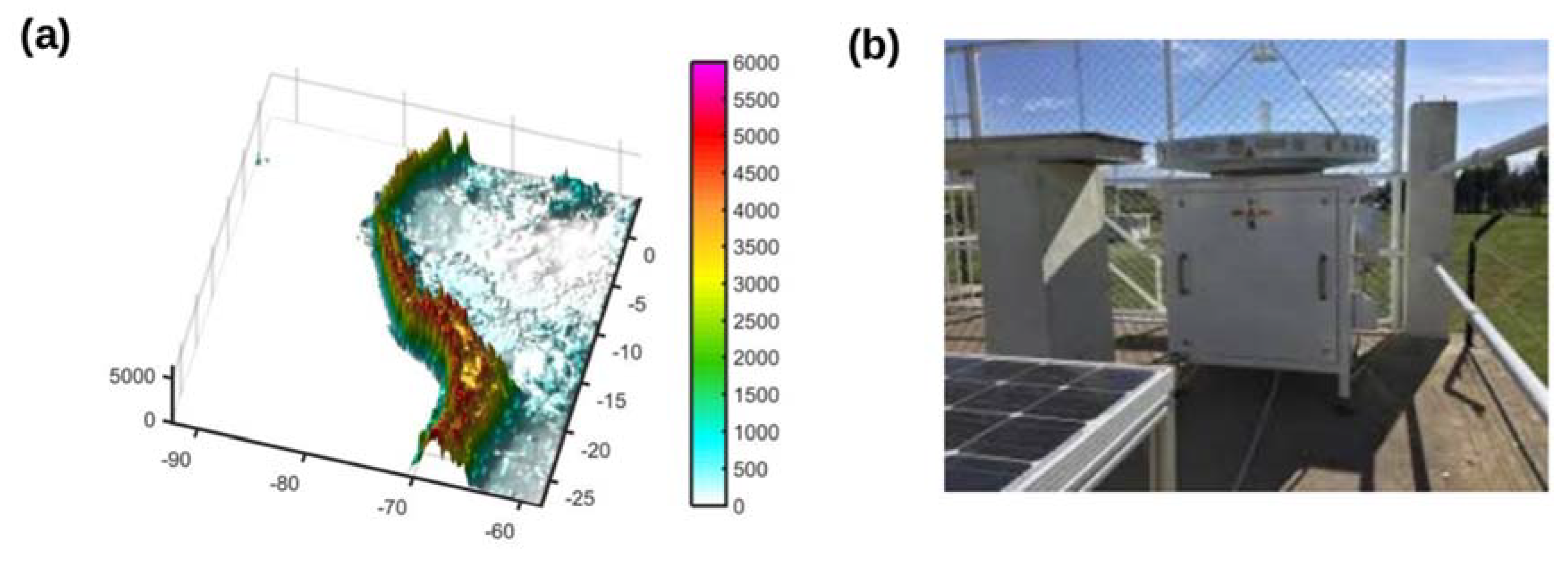
2.1. The Compact Meteorological Ka Band Cloud Radar (MIRA-35c)

MIRA35c is installed at the HYO, located in the center of the Mantaro Basin (MB). MB is located in the central Peruvian Andes (1034′–13°35′ S, 73°55′–76°40′ W) with an area close to 34550 km2. MIRA 35c is a magnetron based pulsed Ka-band Doppler weather radar, and, measures the characteristics associated with the cloud microphysics and rain processes at 34.8 GHz. It transmits the linearly polarized signal and receives co and cross signals simultaneously, to detect the Doppler spectra of radar reflectivity and the Linear De-polarization-Ratio. Both the data could be used to investigate the cloud density and target type respectively [49]. The specifications of MIRA35c are given in Table 1. Many past studies documented the retrieval of Doppler spectra and different rain parameters from VPRR [1,13,14,50]. The primary algorithm follows the Gunn and Kinzer [38] to estimate the fall velocity and DSD parameters. Once DSD parameters are estimated, we derived the attenuated corrected radar reflectivity (Ze) and rain rate following [1,38]. A path integrated rainfall attenuation (PIA) algorithm is applied, using the extinction of DSD at 34.8 GHz [1,38].

2.2. Algorithm Used in the Present Study

Here, MIRA-35C is used to measure the terminal fall velocity of raindrops in the motionless air. To compute the height dependence on drop diameter we followed Gunn and Kinzer [51] and Foote and Du Toit [52], whereas the backscattering cross-section is calculate using Mie theory. Doppler spectra received by VPRR is related to the DSD and given by,
N ( D , z ) Δ D = η ( D , z ) σ ( D ) Δ D
where N(D,z) is the spectral drop density at a height z and (D,z) is the spectral volume scattering cross-section. Single-particle backscattering cross-section, (D), of a sphere with diameter, D, is calculated using Mie scattering theory. Under zero vertical wind assumption, terminal fall velocity of a raindrop, v, can be related to the diameter of falling drops [51] as,
D ( v , z ) = 1 0.6 I n 10.3 9.65 v / δ ( z )
The height dependence of the terminal fall velocity due to change in air density, d(z), is approximated as a second-order polynomial given by,
δ ( z ) = ( 1 + 3.68 × 10 ( 5 ) z + 1.71 + 10 ( 9 ) z 2 )
Therefore, the spectral volume scattering cross-section can be obtained in the Doppler velocity domain as
η ( D , z ) = η ( v , z ) D ( v , z ) v
where g(v,z) is directly obtained from the measured Doppler spectrum. Other rain integral parameters, like rain rate, radar reflectivity and liquid water content (LWC) can be obtained using a standard formulation involving the calculated DSD. The mean fall velocity (v) is calculated directly from the spectral power, p(f), related to the Doppler frequency (f) using the first moment as,
v m = λ 2 0 f · p ( f ) d f 0 p ( f ) d f
At 34.8 GHz, rain attenuation is very severe, especially at a high rain rate. Gaseous attenuation, on the other hand, can be negligible at this frequency due to small path length in the lower troposphere. Therefore, the rain attenuation correction is applied using a recursive algorithm of Kunz [53]. In this technique, all the parameters in the lowest range gate are assumed to have zero rain attenuation. The number density in the lowest range gate is used to estimate the rain attenuation coefficient (kr) for the next range gate. The correction term for two way attenuation (A) in the next range gate will be,
A ( z 2 ) = e x p [ 2 K r ( z 1 ) Δ z ]
Range dependent error is another important consideration in radar remote sensing. Sampling uncertainties due to the beam broadening and weakening of signal strength increase in distance and change in the volume at higher height [54,55]. This kind of error leads to a significant underestimation of radar rainfall [56] in conventional radars. However, here Doppler principle is used to detect the fall velocity, and thus the range-dependent errors will be less. The relation between terminal fall velocity and drop size is mentioned above in the equation. The equation is valid only for stagnant air which is not always a good representation of the natural environment. Since the fall velocity is related to vertical wind motion, any non-zero value of the vertical wind will introduce a bias in the retrieved product. The downwind increases the fall velocity of raindrops leads to an artificial overestimation of the drop size as well scattering cross-section which will ultimately cause an underestimation of the drop density. The rain rate and liquid water content (LWC) will also be underestimated in such a scenario due to a low number of drops. The Doppler retrieval under strong turbulence will, therefore, also be erroneous.
A detailed analysis of the errors caused by such an assumption is given by Peters et al. [1]. It was, however, noted that the improper vertical wind correction would further deteriorate the quality of estimated parameters in comparison to the original retrieved data. Therefore, in this study, the zero vertical wind assumption is used. The VPRR can measure the Doppler spectrum with a minimum time resolution of 10 s and 35 m height resolution. However, radar electronics take nearly 6 s for data processing during which no measurements are possible. To enhance the reliability of data, in this study, VPRR time resolution is set to be 30 s. Further, since the first few range gates in 35 m height resolution can be contaminated by ground echo, the height resolution is fixed at 200 m to cover up to 6 km in 30 steps. With 200 m vertical resolution, the finer rain structure may not be adequately captured, but the mean trend can be captured with good accuracy. At 35 GHz, the attenuation is severe at high rain rate, in some cases, the signal to noise ratio drops to 0 and the signal cannot be corrected, which is possibly the cause of the negative gradient for near surface rain rate ≥20 mm/h below 5 km. On the other hand, on many occasions, the correction of the attenuation overcompensates the signal, which occurs especially in clouds. These constraints are due to significant rain attenuation at a higher rain rate where no attenuation corrections could be applied at the lowest altitude [1,38] and limits our results and capability of instruments. However, our algorithm primarily derived DSD and other rain parameters but does not severely affect the mean fall velocity of the raindrops.
The main concern here is to check the data consistency. To ensure the robustness of the data used in the present study, we checked the data based on a few criteria to minimize the instrumental and other unaccounted errors. First, it is assured that derived individual vertical profiles must be complete and no discontinuity should be there. These limitations constrain the error due to sudden reflections arising from insects or non-hydrometeors. We also compared to radar data with the disdrometer data to check the discrepancy in the rain pattern. For comparison purposes, accumulated rainfall is obtained at the lowest height range from VPRR [13,14]. When we compared the VPRR with rain gauge data, the rain gauge shows the higher rainfall values compared to VPRR (Figure 2a), although a good agreement is observed between two data sets [38] (Figure 2b). However, a decay in the Ze is observed at a very high rain rate similar to that observed in [1,38] and some clouds (vertical profiles) are overcorrected (Supplementary Materials Figure S1).
Figure 3 shows an example of the vertical profile of Ze measured through VPRR. In the first case (Figure 3a) the Ze pattern shows the highest Ze values near the surface between 23 UTC (18 LT) to 02 UTC (21 LT). The Ze values are more than up to 40 dBZ in the first few kilometers above the surface, but Ze value decreases drastically (−15 dBZ) at a higher altitude. It indicates the larger number of hydrometeors (rain and hail). In the second case (13 December 2017) the VPRR captured the stratiform regimes of the cloud systems with the well defined bright band (~4.7 km altitude). Above 5 km the Ze values are less than 15 dBZ and indicate the light rain and drizzle. An anvil structure is also observed, where a lower Ze is observed at >6 km, with no significant Ze values at the lower altitude and indicates the anvil precipitation structure [57].

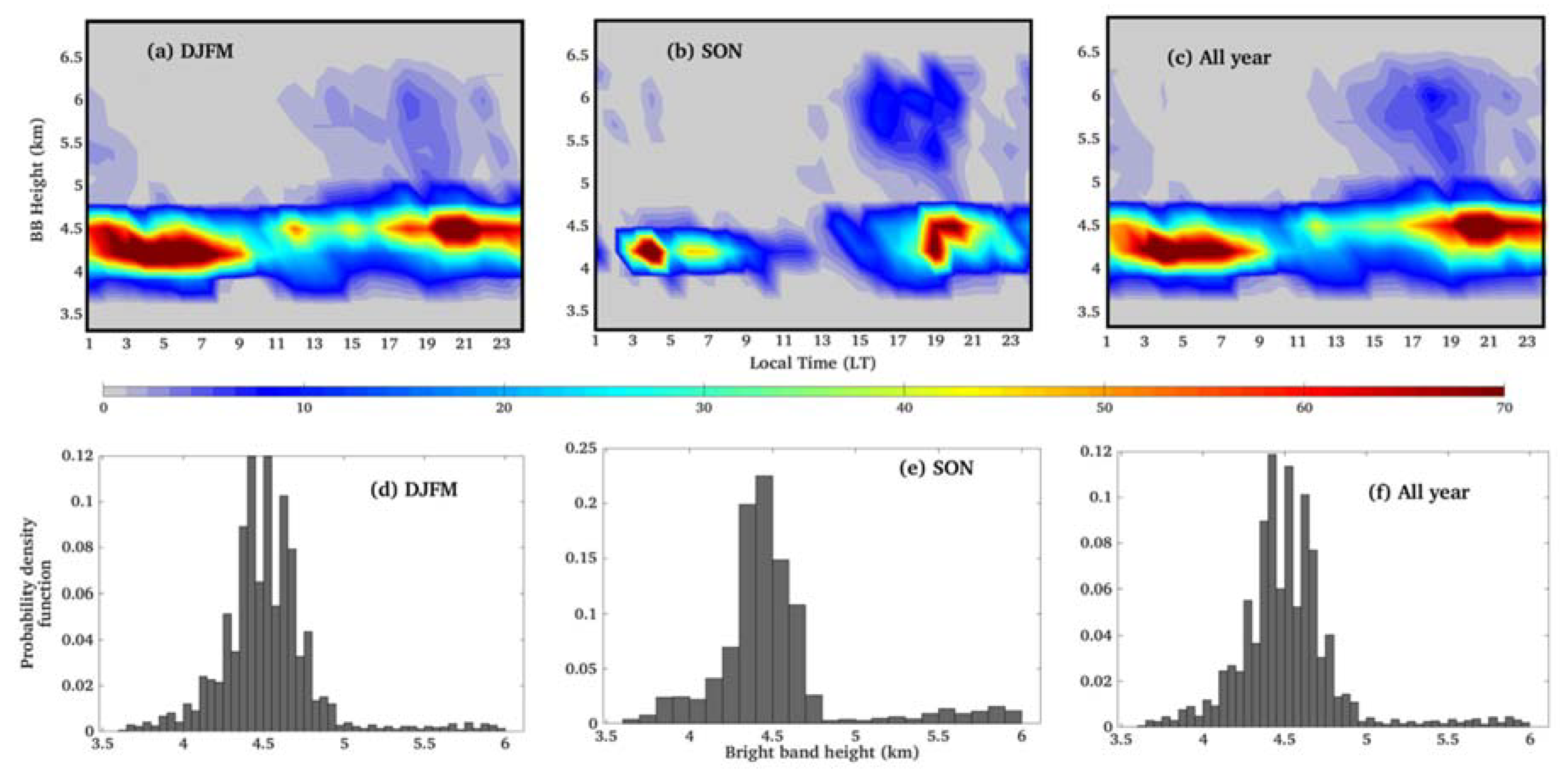
2.3. Bright Band Height Detection

The bright band plays a vital role in deciding the DSD parameters and consists of a layer of increased Ze followed by an increase in Doppler velocity near the ML [58]. Whenever snow crystals fall below the 0 °C, they begin to melt, and increase the Ze below the ML and provides the bright band mainly in stratiform precipitation. Once the melting is completed, the raindrops have a smaller diameter than the snowflakes and attain the terminal velocity [59]. The vertical profile of Ze could be used to identify the bright band height [18,60,61,62,63,64]. For example, Endries et al. [18] developed an algorithm to calculate the top and bottom of the melting layer. The altitude with the most negative gradient in Ze and Doppler velocity is termed as the top and bottom of the ML, respectively [18,61]. The bright band height in the present study is calculated for each vertical Ze profile [61], see Figure 3. Basically, the most negative gradient in Ze profile is used to estimate the bright band height [18,60]. In the present study, a derived bright band height is discarded from the present study, when bright band height was above 6.5 km and less than 3.5 km (implausible under current tropospheric conditions).

2.4. Vertical Structure of Rain (VSR) at Different Rain Rate

VPRR data are validated in the past over different regimes of the globe in the rainy areas [1,13,14,62,63,64], and revealed the VSR depends on the near-surface rain rate. To investigate the mean vertical structure of rain, we followed the methodology described in [1,38]. Here, near-surface rain rate is divided into four categories, namely 0.02–0.2 mm/h, 0.2–2 mm/h, 2–20 mm/h and 20–100 mm/h [1,38]. This methodology is selected since rain structure strongly depends on the rain type, namely convective and stratiform rain [1,38,65]. There are various other methodologies available to distinguish between stratiform and convective rain, however rain rate is commonly used to classified the different rain types. To investigate the rain structure vertical profiles of rain rate, LWC, Ze and DSD parameters are drawn at different near-surface rain rate.

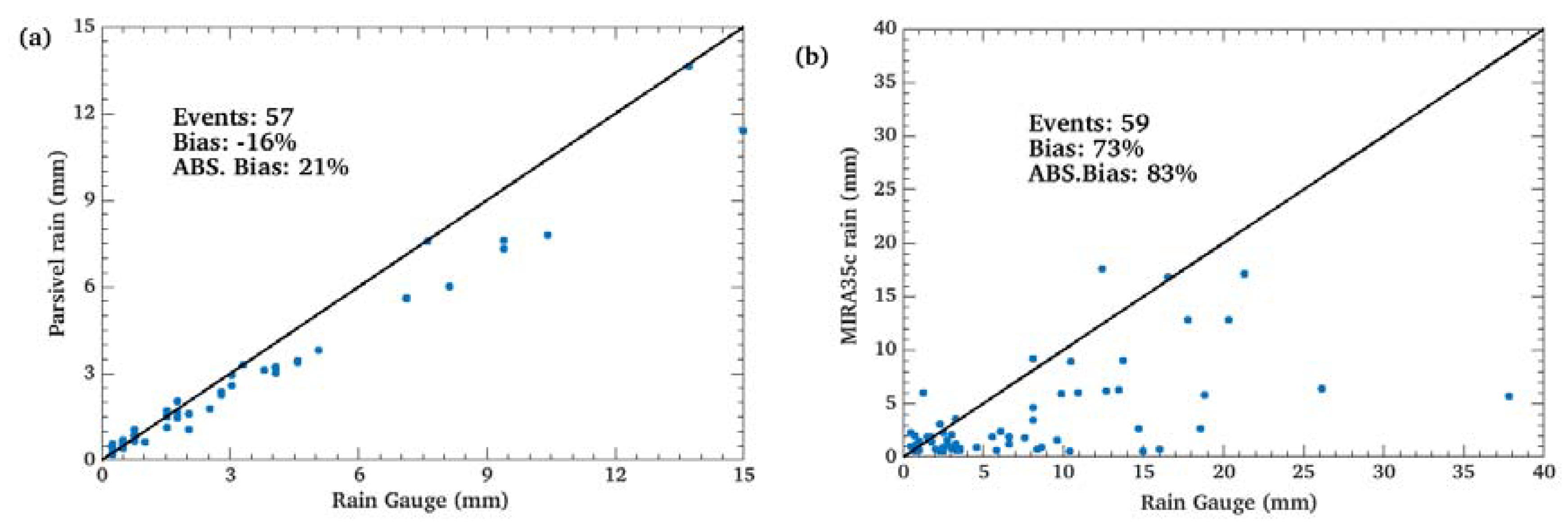
2.5. Field Campaign and Reanalysis Data

A field campaign is launched over HYO between 18 February to 14 March 2019. Several ground-based instruments including radiosonde, rain gauge and VPRR data are used to investigate the convective and stratiform rainfall mechanism. We also used the reanalysis data GFS at 1° × 1° grid resolution at different pressure levels to investigate the dynamical behavior of the atmosphere during the convective and stratiform rain events. The overall data used in the present study is listed in Table 2.

3. Results

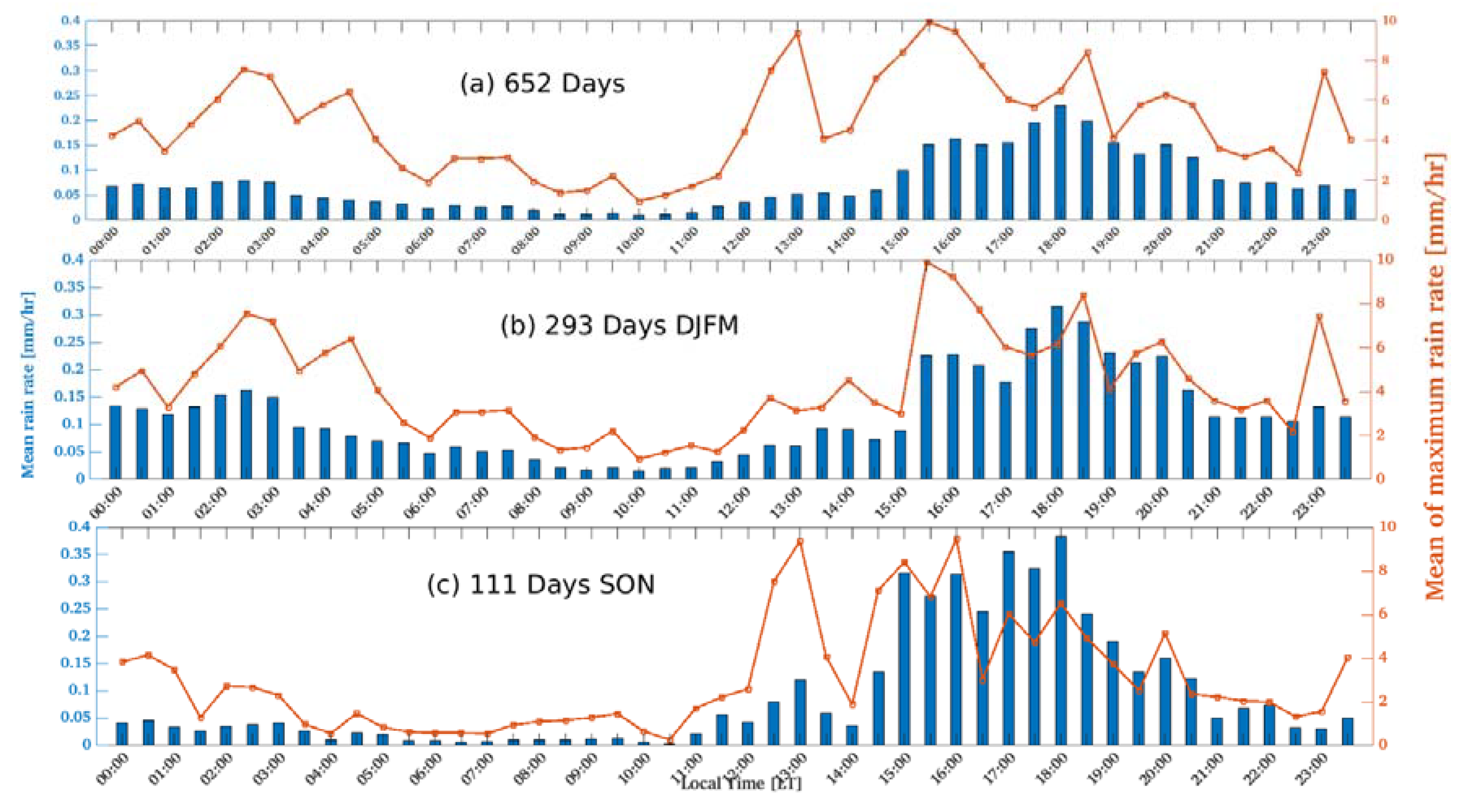
3.1. Diurnal Variation of Rainfall and Bright Band

Figure 4 shows the diurnal variation in the surface rainfall during the study periods. The mean and maximum of rain rate follow the diurnal patterns, and, consistent with the past study over the other locations over the tropical Andean [10,18,27]. The mean rain rate consists of the two maxima namely afternoon (17:00 to 19:00 LST) and midnight hour (1:00 to 3:00 LST). However, the mean of maximum rain rate has several maxima during the study periods. DJFM and SON have similar trends, however, the mean rain rate is higher during SON (~0.4 mm/h) months compared to DJFM months (~0.35 mm/h). The difference between afternoon and mid-night maxima is higher during SON compared to DJFM and indicates that most of the rainfall maxima occur during the afternoon, and could be related to topographical condition and diurnal variation of the surface temperature rather than the seasonal variation [19,20]. For example, the mean rain rate peaks (has higher rain rate values) at ~0.35 mm/h and 0.18 mm/h in the afternoon and early morning during DJFM months respectively, whereas corresponding values are ~0.4 mm/h and ~0.05 for SON months in afternoon and early morning, respectively. Second, the DJFM months have a clear maxima at 18:00 LST, and, then decreases around 18:00 LST, whereas maxima in mean rain rate spread for the time between 15:00 to 18:00 LST during SON months.
Figure 5 shows the diurnal variation (a–c) and probability density distribution (d–f) for bright band height. It is observed that bright band height is higher during the summer monsoon season compared to pre-monsoon seasons. The bright band height mostly lies between 4 to 5 km altitude. This is somewhat consistent with the past studies and observed bright band height for the other stations over the Andes mountain [17,18,37]. The probability of bright band height decreases sharply after 5.0 and 4.7 km during DJFM and SON seasons respectively. However, irrespective of the diurnal cycle more than 70% of bright band lies less than the 5 km altitude, and only less than 20% bright band height is smaller than 5 km altitude. The probability density distribution of bright band shows the seasonal variation. For example, DJFM months have the two peaks (~4.4 and ~4.6 km), whereas SON has a single peak near 4.5 km altitude, and, the maximum height of bright band lies between 4.2 to 4.6 km altitude. The bright band height shows the role of solar heating at the higher topographic areas [17,18,37]. For example, first, the higher density of bright band with higher altitude found either afternoon or evening. Although, there is a possibility that bright band could rise more than 5 km, mostly in the afternoon and late-night (13:00 LST to 23:00 LST), and follow a heating pattern over the tropical Andes [17,18,37].
Table 3 provides a detailed information of the bright band height observed during the different times of a day. The seasonal differences are not pronounced, but still diurnal variations are evident. Midnight, afternoon and overnight times of a day show the variation of 500 to 900 m in bright band height. For example, mean bright band height is highest (~4.66 km) during SON months between 14:00–19:00 LST followed by DJFM months (~4.62 km) between 20:00–01:00 LST. Although the highest median bright band height (~4.57 km) observed in DJFM months between 20:00 to 01:00 LST and standard deviation is higher during SON months for bright band height.

3.2. Vertical Structure of Rain

Figure 6 shows the vertical variation of Ze, rain rate and LWC (gm−3) during DJFM and SON months for different rain rate classes. It is observed that monsoon months consist of an intense Ze vertical profile compared to pre-monsoon seasons, whereas in the mixed-phase altitude (6–9 km) the average Ze is higher during SON seasons except for rain rate ≥20 mm/h. The maximum differences in average Ze profiles occur between the mixed-phase regimes, whereas above the 9 km altitude, the average Ze profiles merge and consistent with the longterm TRMM and GPM observations [40,66,67,68,69,70,71]. For the near-surface rain rate <0.2 mm/h, the average Ze profiles have a negative slope and Ze decreases with the height through all the vertical column [40,72]. However, in general, the average Ze profiles can be divided into two regions, e.g., below and above the 5.0 km altitude (very near to 0 °C; Figure 6a). Below the 5 km altitude, the average Ze either increases, decreases or remain constant with the altitude, and depend on the different class of RR. However, above 5 km, the average Ze decreases as the altitude decreases for all classes of RR. Within the lowest, ~1 km altitude near the surface, the average Ze is highest for rain rate ≥20 to 200 mm/h and least for rain rate ≤0.02–0.2 mm/h. Above the 5 km altitude, average Ze shows the different characteristics, and least for the near-surface rain rate ≥20 mm/h during DJFM months, which is related to the attenuation issue discussed earlier [1,38]. The opposite slope of Ze below and above the 5 km altitude, are related to the growth and decay of the hydrometers in cloud systems and depends on the cloud microphysical processes [67,68,69,70,71,72].
Figure 6b shows the average vertical profile for different classes of near-surface rain rates. The seasonal differences are observed as x-axis is on the logarithmic scale. For example, DJFM months average vertical profiles have more intense average rain rate profiles compared to premonsoon seasons except for the rain rate ≥20 mm/h above 4.5 km altitude. For the near-surface rain rate ≤2 mm/h, average rain rate profiles have a positive slope e.g., average rain rate increases up to 5 km altitude from the surface and then either decrease slowly (negative slope) or remains constant. These findings are consistent with the other studies using VPRR over the different regimes of the globe [1,38,64,73]. SON months show the different characteristics compared to DJFM months for the rain rate ≥20 mm/h and the reason is not clear. Maybe the mixed rain during the transition periods/phase from convective to stratiform rain, where local convection or convective systems could become stratiform precipitation very quickly [38]. The transported moisture in the upslope and easterly flow [10] and the rising moist airflow along the slope, simulate the condensation and raindrops start falling and enhance the local precipitation [74]. The opposite slope below the ~4.5 km for rain rate ≤0.2 mm/h, reveals that small-sized of hydrometeors are not able to reach the surface, and, evaporation of small size of hydrometeors are effective for the lowest class of rain rate [19,20,28].
Figure 6c shows the vertical variation of LWC for the different classes of rain rate and shows similar features as observed in average rain rate profiles. For example, monsoon seasons have higher LWC compared to pre-monsoon months. Again, the average LWC is least for DJFM months above 4.5 km altitude for RR ≥ 20 mm/h and similar to that observed in rain rate and Ze profiles. For the lowest class of rain rate <0.2 mm/h, the LWC has a positive slope (dLWC/dz > 0) up to 5 km altitude and then either remain constant or consist of the negative slope above the 5 km altitude. These findings are consistent with the earlier study over the higher altitude regimes over the Indian subcontinent [38]. The negative slope for higher rain rate is expected due to overcompensation of the rain attenuation at higher rain rate [38]. However, the positive slope in LWC for less rain rate, indicates the correct estimation, and, errors are very less due to rain attenuation in the lower rain rate. The possible regions behind such behavior are the shift of the DSD peak, where DSD parameters consist of smaller drops at higher altitude and are explained deeply in the next section. The lowest class of rain rate generally associated with the drizzle (with Ze < 0 dBZ) and related to the shallow clouds with less fall velocity and smaller raindrops [1,73]. Evaporation also plays a significant role at low rain rate and at the lower altitudes which affects the smaller drops concentration and mentioned in the next section.

3.3. Distribution of DSD Parameters

Figure 7 shows the vertical profile of DSD parameters for different classes of near-surface rain rate. The vertical variation of the DSD during premonsoon and monsoon months shows nearly similar features. In general, different class of rain rate show similar trends, and, a higher concentration of larger sized drops is observed near the surface. However, a higher concentration of less sized of hydrometeors is observed at higher altitude. In a minor difference, the seasonal differences are evident, as DJFM have a higher concentration of bigger raindrop for different classes of rain rate especially for RR ≥ 0.2 mm/h compared to SON months. Below we will discuss the DSD vertical growth for the different classes of near surface rain rate.
For the lowest class of rain rate (0.02–0.2 mm/h), the droplet of size Dm < 1 mm has a higher concentration and dD/dZ remains constant below the freezing height. But the droplet of size Dm < 0.5 mm shows the opposite characteristics during JJAS and SON seasons. For example, the droplets of less than 0.5 mm have a negative trend (dD/Dz < 0), just below the freezing level during SON season, and indicates the drop break up or evaporation mechanism in the lowest rain rate class (0.02–0.2 mm/h). But this feature is not visible during DJFM months. This could be because of the sufficient moisture supplied by the SA–LLJ and surface flow from the Amazon basin towards the Andes mountain during JJAS months [19,20,21]. Although the total number of smaller drops (Dm < 1.0 mm) remain constant within the mixed-phase regimes and increases below the freezing level during both the seasons. In addition, a higher concentration of higher sized of droplets below the ML could be because of moisture loaded surface flow and SA-LLJ [10,41]. The negative gradient for the small droplets is consistent with the studies over the Western Ghats over South Asia [75].
For the rain rate lies between 0.2–2 mm/h, the DSD parameters reveal the dominance of the collision-coalescence mechanism and a higher concentration of bigger droplets (Dm > 1 mm) are observed below the ML during both the seasons and even higher during DJFM months. The concentration of the fewer droplets (Dm < 1 mm) also increases in the lowest height (<1 km; near the surface). Although in a small difference, SON shows the decreases in the concentration for Dm < 0.5 mm and indicates the evaporation of the smaller droplets. For the rain rate lies between 2–20 mm/h, the differences are higher above and below the ML compared to the lower class of near-surface rain rate. A higher droplet concentration of larger size of droplets (Dm > 4 mm) is observed near the surface compared to previous cases. However, in a small difference SON has a higher fraction of droplets with Dm < 0.5 mm below the ML. Since the rain rate between 2–20 mm/h belongs to both types of rain (e.g., convective and stratiform precipitation), the drop evolution mechanism namely collision-coalescence and break up are effective. The collision-coalescence process produces the higher sized of hydrometeors below the freezing level [38], whereas evaporation could lead to less sized hydrometeors (Dm < 0.5 mm). The presence of smaller droplets with a higher concentration at the lower rain rate could be associated with the bright band feature, where bright band events contribute to DSD at smaller rain rate [76]. The raindrops that originate from the bright band could have less liquid water content and may contribute the less rainfall just below the ML height. They also undergo the collision-coalescence and affect the total rainfall near the surface, and thus a sudden increase in droplets is observed just below the ML.
For rain rate ≥20–200 mm/h, a higher concentration of droplets with Dm < 2 mm are observed above the ML compared to other classes of rain rate. The role of orographic upward-wind is evident, and most of the small-sized of raindrops are removed due to strong wind and also consistent with the other tropical locations [31,56]. At the same time, a higher concentration of bigger raindrops (Dm ≥ 4 mm) is observed in the lowest regimes of the altitude compared to other class of near-surface rain rate. Since the rain rate ≥20 mm/h mostly corresponds to convective rainfall and consists of the evolution of bigger raindrops near the surface. These observations indicate that there is a much higher possibility of collision-coalescence processes at the lower height range, whereas the ice microphysics are responsible for bigger raindrops within the mixed-phase regimes [12,14,17]. HYO is located at ~3.2 km above the mean sea level and very near to the bright band height, and, once the snow or ice crosses the 0 °C height, they melt and create the bigger raindrops, which falls quickly to contribute to higher near-surface rain rate. Gatlin et al. [74] used ground-based radar data and explained that a thick bright band height, causes an enhancement in raindrop size below the bright band and also extends up to the surface. Several studies also revealed that larger raindrops were observed at the ground because of intense Ze values in the bright band. The constant cloud base layer within the boundary layer affects the DSD variations [76] whereas internal dynamics (shallow layer with the upper layers) at the tops of the hills contribute to the number-controlled processes (e.g., collision-coalescence and breakup). In dynamic equilibrium, these processes produce the smaller raindrops and show a uniform vertical profile at high-altitude regions [38,75].

4. Campaign Periods over Huancayo

Figure 8 shows the daily accumulated rainfall during campaign periods (e.g., 18 February to 14 March 2019). The rainfall can be divided into dry and wet spells (4 March to 10 March 2019). 16.3 mm rainfall was recorded within the 24 h on 10 March, followed by 7 March and 25 February 2019, with 12.2 and 10 mm of accumulated rainfall respectively. In the next section, we will use the in situ observations and reanalysis data to investigate the atmospheric variability to produce the rainfall events.

4.1. Vertical Profiles of Reflectivity during the Rainy Periods

Figure 9 shows the vertical profile of air temperature collected between the 3rd to 11th March in the early morning (07 LST) and afternoon (19 LST) along with a dry and moist lapse rate. The observed temperature profiles are nearer to the moist lapse rate during the nighttime. There is no significant inversion mechanism is observed during the wet spells, and, all the temperature profiles cross the 0 °C only once. The 0 °C lies between 5250 and 5550-m which is nearly 150–200 m higher than the observed climatological bright band (Figure 5). These results are consistent with the past finding [59], where bright band existed 253 m below the 0 °C level because of the time taken by the frozen hydrometeors to melt with respect to ambient temperature. Figure 10 shows the vertical profile of Ze collected during wet spells. It is observed that most of the rainy days consist of the cloud systems with a well defined bright band [18] in stratiform precipitation. Although few convective events are also observed and tabulated in Table 4 [21]. For example, 10 March has the highest accumulated rainfall (16.8 mm) and consists of a clear bright band structure between 4:00 to 6:30 UTC, whereas, intense convection is observed at 23:40 UTC and lost for nearly 3 h.

4.2. Convective and Stratiform Rainfall Activity

To investigate the microphysical and dynamical behavior during the convective and stratiform rainfall events, two convective and two stratiform precipitation events (CPEs and SPEs) are defined (Table 4). It is observed that CPEs have much higher accumulated surface rainfall compared to SPEs [18,19,21]. For example, the first CPE produces ~7.4 mm of accumulated rainfall in one hour (19:00 to 20:00 UTC on 7th March) whereas second CPE produces ~2.01 mm of rainfall within one and half hour. The SPEs show the different characteristics compared to CPEs and lost for many hours, but produce less accumulated surface rainfall. For example, first SPE observed on 7th March between 00:00 UTC to 10:00 UTC and only produces 3.55 mm of accumulated rainfall with median bright band height at ~4.56 km. The second SPE lost for ~8 h (00:00 UTC to 07:30 UTC) and contributes ~1.01 mm of accumulated rainfall with bright band height occurred ~4.70 km.
Figure 11 shows the wind-stream lines at 18:00 UTC for at lower (950, 850 hPa), mid (700, 500 hPa) and upper-pressure levels (200 hPa) for 7th and 10th March. The wind circulations show different characteristics during two CPEs and SPEs. For example, a well-defined north-easterly circulation was observed along the east side of the Andes that follows the SALLJ at 850 and 950 hPa on 7th March 2019 (Figure 11a). These north-easterly circulations favor the intrusion of moisture from the Amazon basin to the central Andes. In contrast, on the 10th March (Figure 11b) the easterly circulations are restricted at low latitude (around 15° S), probably due to the disturbance produced by two anticyclonic circulations centered at (20° S, 50° W) and (40° S, 58° W). The last anticyclonic was also observed at 850 and 950 hPa and is probably associated with the south-west displacement of the South-Atlantic high-pressure system (Figure 11b), which favors the south-easterly circulations along the east side of the Andes that could disfavor the intrusion of moisture from the Amazon basin to the central Andes.
The characteristics of the CPEs depend on the static stability of the environment, wind speed and wind shear [77]. Sounding results between 06–11 March at 07 and 19 LST are shown in Figure 12, whereas sounding results at 13 LST are shown in Figure 13. For all the rainy days, a stable atmosphere is observed at 07 LST that creates an air potential temperature gradient (θ) directed towards the surface with values between 315 K and 320 K near the surface. On 7, 8 and 10th March, a negative gradient in the equivalent potential temperature (θe) was observed at 07 LST, which indicates a slightly conditionally unstable layer in the first 4 km, and probably caused by a presence of high moisture content in these days with surface value of θe near to 340 K. In contrast, at 13 LST a highly unstable condition was observed, with higher negative gradients in θe on 07, 10 and 11 March. However, the release of conditional instability occurs only when θe is almost equal to θe* (saturation equivalent potential temperature) near the surface. This situation was observed on 07 March at 1500 m, on 08 March at 3000 m and on 09 March at 2500 m.

5. Conclusions and Limitations

The VSR at the HYO provides an important feature of the tropical rain and reveals the important consequences in space-based radar retrieval of precipitation. Our results support that the vertical structure of radar reflectivity, rain rate, and LWC show the different characteristics below and above the ML. They consist of a sharp gradient due to the bright band and the melting of the ice. A strong vertical variation is observed for the higher rain rate ≥20 mm/h and vertical variation in the DSD is responsible for them. The drop evolution mechanism is observed and it is shown that that in general drop break-up mechanism is dominant in stratiform rain whereas the collision-coalescence process is active in convective rain. In situ observations and reanalysis data show the role of the atmospheric condition in generating the different types of rainfall. Our analysis clearly reveals the higher afternoon and nighttime precipitation with higher bright band height, which partially attributes to strong daily fluctuations in surface temperature that tropical Andes experience. This is consistent with the past studies over the other site of the tropical Andes [17,18,25,31,37]. Minima in the precipitation and bright band height are observed in the early morning hours as surface temperature approach a diurnal low. The bright band height was highest in the afternoon and could be associated with a deep, well-mixed planetary boundary layer. This convection also resulted in local maxima in rain rate and maxima of VPRR-detected precipitation during these hours (Figure 4 and Figure 5).
In situ observations and the climatological behavior during the rainy days clearly show the dominance of stratiform precipitation with a well-defined bright band structure [17,27,30,37,78] and indicates the weaker air motion [58,79]. The previous studies also suggested that afternoon and nighttime precipitation in the region are associated with mesoscale convective systems (MCSs; [10,27,28,47,80]). These MCSs are formed at the lowland due to the response to daytime heating and convergence of downslope flow after sunset [27,28]. A day time heating over the mountain induces an upslope valley breeze and initiates the precipitation under the higher moisture flux [25]. The interaction between the Amazonian moisture and evaporatively cooled downslope flow during the precipitation in the mountain slope also persists the precipitation in the Andes mountain valley [25,26,27,28]. However, in the absence of overnight and nighttime cloud, the interaction between the radiatively cooled downslope flow and Amazonian moisture also contribute to nighttime precipitation peak in the valleys [25,27,29]. Orographic influence also affects the rainfall in the Andes mountain valley and consists of the seeder–feeder mechanism which could enhance the stratiform precipitation structures [17,37]. This allows the afternoon convection and further evolves into broader, long-lasting stratiform systems that persist through the night. Based on the present study the major findings are mentioned below:
  • A bimodal pattern is observed in precipitation and bright band height with local maxima during after-noon and overnight. This is partially attributed to the diurnal cycle of surface temperature in the tropical Andes.
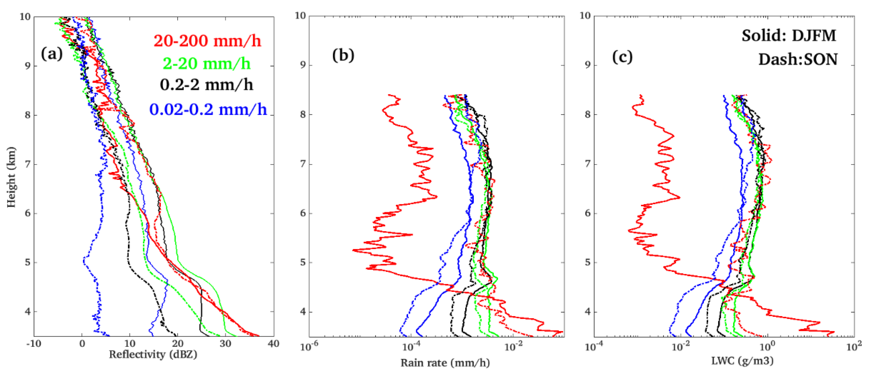
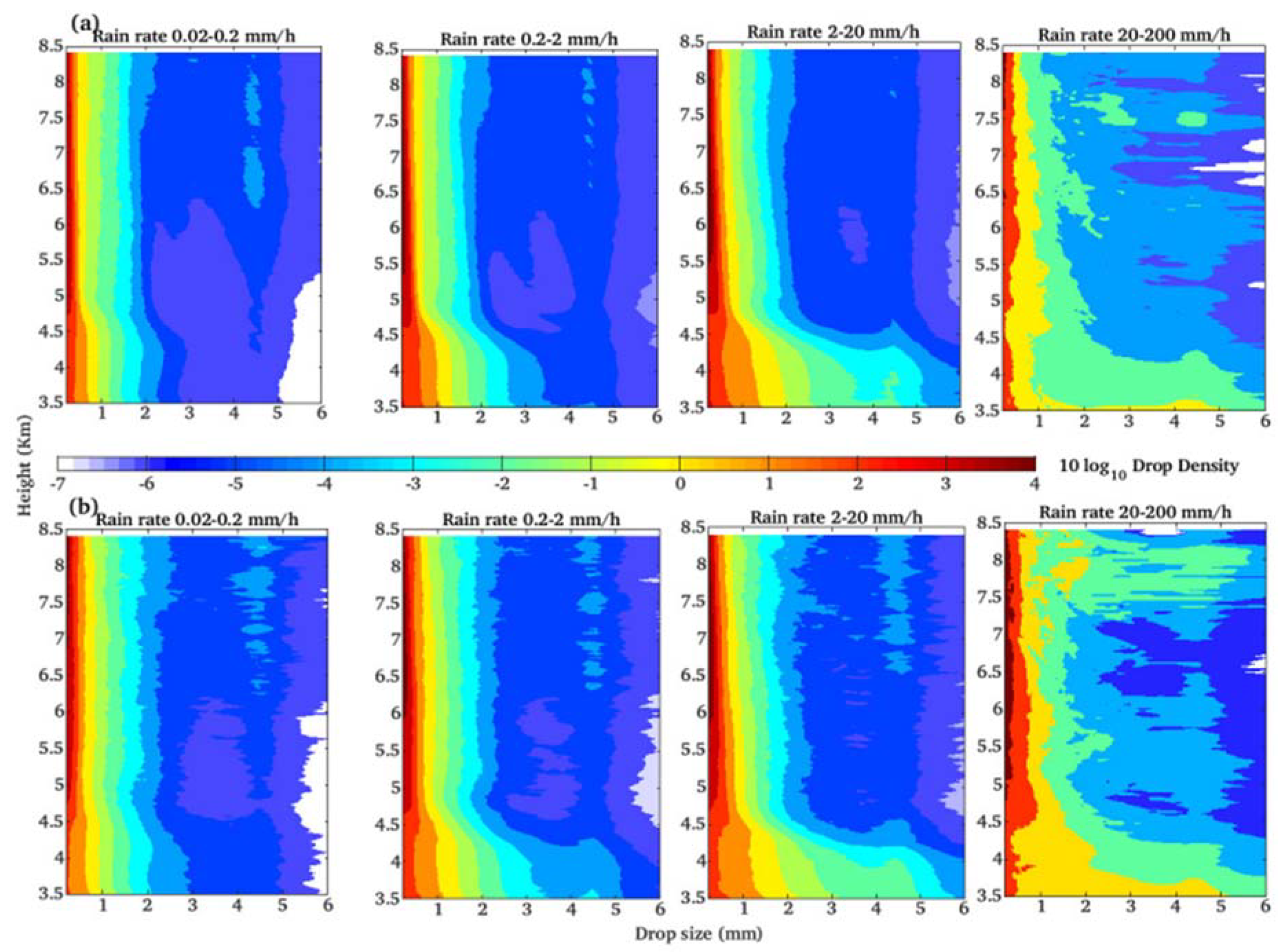
  • The average Ze profiles show the gradient near the freezing height due to the melting layer and for the higher near-surface RR, Ze decreases sharply above the freezing height. Rain rate and LWC show the different vertical variations below and above the 6 km altitude. The DSD variation shows the higher concentration of larger sized of drop for higher near-surface rain rate below the ML. Although the dominant mode of drop size is less than 1 mm for most of the near-surface rain rate.
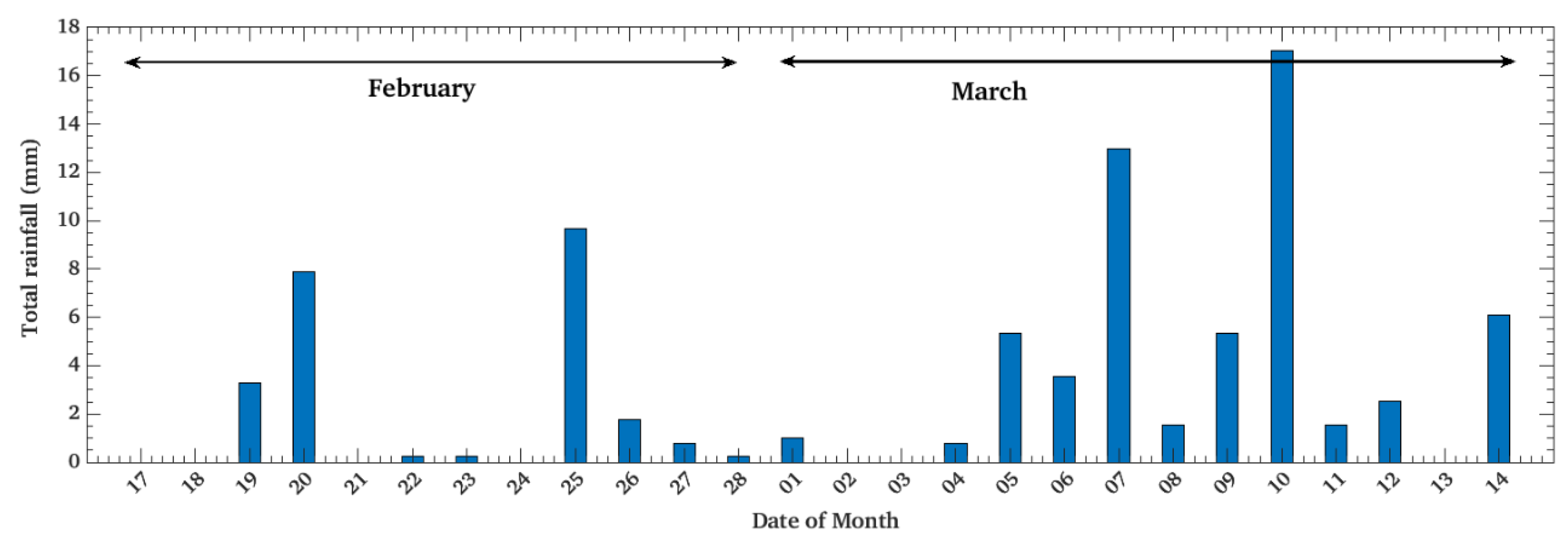
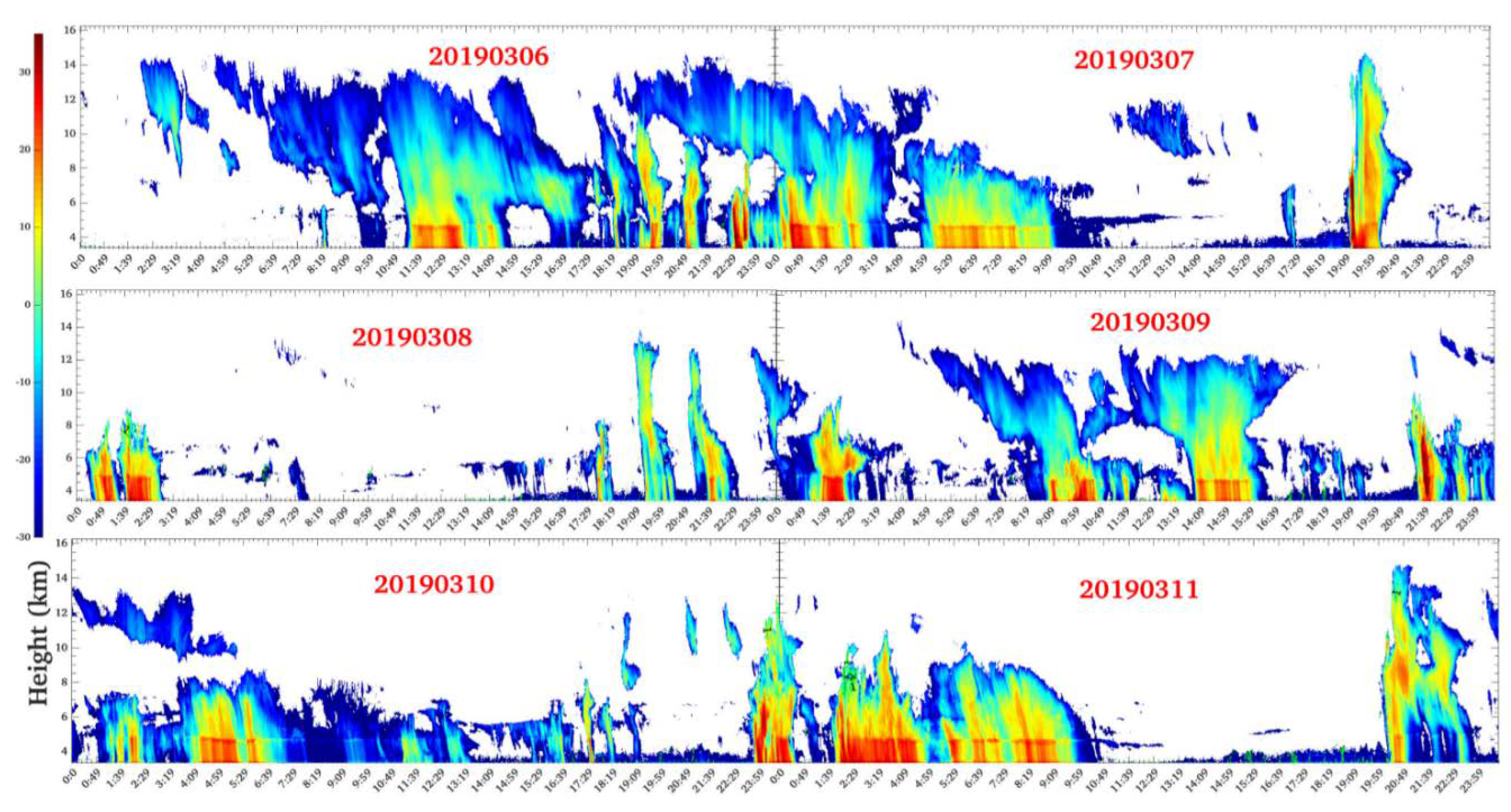
  • The rainfall characteristics during campaign periods reveal the convective organization with higher precipitation. However, stratiform precipitation was more common and exist for the longer periods, but with less accumulated surface rainfall.
The present study improves the understanding of rainfall characteristics over the tropical Andes. However, many uncertainties affect the outcome. For example, a VPRR can only observe the hydrometeors, which pass over it and could miss the intense regimes of the cloud systems. Another issue is the algorithm used in the present study and discussed earlier. Peters et al. [1] explained that the negative slope in higher rain rate is expected, because of overcompensation of the rain attenuation at higher rain rate [38]. However, the positive slope in the LWC shows the correct estimation and errors are very less in this rain rate range due to rain attenuation. The possible regions behind this kind of behavior are the shift of the DSD peak toward smaller drops with increasing height. The lowest class of rain rate generally associated with the drizzle (with Ze < 0 dBZ, Houze [81]) and related with the lower shallow clouds and with less fall velocity and smaller drops [11,73]. At the same time, evaporation also plays a significant at very low rain rates and affects the small raindrops concentration. However, the further research is required to find the relationship between convection initiation with the diurnal heating in the region and then its development into the organized precipitation and their impact on the tropical Andes weather and climate. In addition, the simultaneous observations and larger time-series data from the ground-based observations would help to investigate the relationship between the geography and atmospheric patterns on the local precipitation.

Supplementary Materials

The following are available online at https://www.mdpi.com/2073-4433/11/3/248/s1. Figure S1. A particular example of the PIA algorithm.

Author Contributions

S.K.: conceptualization, validation, methodology, data analysis, Field campaign supervision, radar data concept, Algorithm development and wrote the original draft; C.D.C.-V.: Data analysis, validation, methodology and wrote the original draft; J.M.V.P.: validation, handled the Radar data; J.L.F.R.: Data analysis, validation and wrote the original draft; S.M.C.G.: Collected the field data and data analysis; A.S.M.A.: Edited the manuscript; D.M.-C.: Edited the manuscript; Y.S.: Funding acquisition , Edited the manuscript. All authors have read and agreed to the published version of the manuscript.

Funding

This research was funded by the “Consejo Nacional de Ciencia y Tecnologia” (CONCYTEC) grant number 010-2017-FONDECYT and by the “INNOVATE PERU” grant number 400-PNIC-2015.

Conflicts of Interest

The authors declare no conflict of interest.

References

  1. Peters, G.; Fischer, B.; Münster, H.; Clemens, M.; Wagner, A. Profiles of raindrop size distributions as retrieved by microrain radars. J. Appl. Meteorol. 2005, 44, 1930–1949. [Google Scholar] [CrossRef]
  2. Thurai, M.; Iguchi, T.; Kozu, T.; Eastment, J.D.; Wilson, C.L.; Ong, J.T. Radar observations in Singapore and their implications for the TRMM precipitation radar retrieval algorithms. Radio Sci. 2003, 38, 1086. [Google Scholar] [CrossRef]
  3. Kirstetter, P.E.; Andrieu, H.; Boudevillain, B.; Delrieu, G. A physically based identification of vertical profiles of reflectivity from volume scan radar data. J. Appl. Meteorol. Climatol. 2013, 52, 1645–1663. [Google Scholar] [CrossRef] [Green Version]
  4. Cluckie, I.D.; Griffith, R.J.; Lane, A.; Tilford, K.A. Radar hydrometeorology using a vertically pointing radar. Hydrol. Earth Syst. Sci. 2000, 4, 565–580. [Google Scholar] [CrossRef]
  5. Koistinen, J.; Michelson, D.B. BALTEX weather radar-based precipitation products and their accuracies. Boreal Environ. Res. 2002, 7, 253–263. [Google Scholar]
  6. Bellon, A.; Lee, G.W.; Kilambi, A.; Zawadzki, I. Real-time comparisons of VPR-corrected daily rainfall estimates with a gauge mesonet. J. Appl. Meteorol. Climatol. 2007, 46, 726–741. [Google Scholar] [CrossRef] [Green Version]
  7. Seo, D.J.; Breidenbach, J.; Fulton, R.; Miller, D.; O’Bannon, T. Real-timeadjustment of range-dependent biases in wsr-88d rainfall estimates due to nonuniform vertical profile of reflectivity. J. Hydrometeorol. 2000, 1, 222–240. [Google Scholar] [CrossRef]
  8. Zipser, E.J.; Lutz, K.R. The vertical profile of radar reflectivity of convective cells: A strong indicator of storm intensity and lightning probability? Mon. Weather Rev. 1994, 122, 1751–1759. [Google Scholar] [CrossRef] [Green Version]
  9. Bellon, A.; Lee, G.W.; Zawadzki, I. Error statistics of VPR corrections in stratiform precipitation. J. Appl. Meteorol. 2005, 44, 998–1015. [Google Scholar] [CrossRef] [Green Version]
  10. Kumar, S.; Silva-Vidal, Y.; Moya-Álvarez, A.S.; Martínez-Castro, D. Effect of the surface wind flow and topography on precipitating cloud systems over the Andes and associated Amazon basin: GPM observations. Atmos. Res. 2019, 225, 193–208. [Google Scholar] [CrossRef]
  11. Kozu, T.; Reddy, K.K.; Mori, S.; Thurai, M.; Ong, J.T.; Rao, D.N.; Shimomai, T. Seasonal and diurnal variations of raindrop size distribution in Asian monsoon region. J. Meteorol. Soc. Jpn. 2006, 84A, 195–209. [Google Scholar] [CrossRef] [Green Version]
  12. Rao, T.N.; Radhakrishna, B.; Nakamura, K.; Rao, N.P. Differences in raindrop size distribution from southwest monsoon to northeast monsoon at Gadanki. Q. J. R. Meteorol. Soc. 2009, 135, 1630–1637. [Google Scholar]
  13. Das, S.; Maitra, A.; Shukla, A.K. Rain attenuation modeling in the 10–100 Ghz frequency using drop size distributions for different climatic zones in tropical India. Progr. Electromagn. Res. B 2010, 25, 211–224. [Google Scholar] [CrossRef] [Green Version]
  14. Das, S.; Shukla, A.K.; Maitra, A. Investigation of vertical profile of rain microstructure at Ahmedabad in Indian tropical region. Adv. Space Res. 2010, 45, 1235–1243. [Google Scholar] [CrossRef]
  15. Francou, B.; Vuille, M.; Wagnon, P.; Mendoza, J.; Sicart, J.-E. Tropical climate change recorded by a glacier in the central Andes during the last decades of the twentieth century: Chacaltaya, Bolivia, 168S. J. Geophys. Res. 2003, 108, 4154. [Google Scholar] [CrossRef]
  16. Salzmann, N.; Huggel, C.; Rohrer, M.; Silverio, W.; Mark, B.G.; Burns, P.; Portocarrero, C. Glacier changes and climate trends derived from multiple sources in the data scarce Cordillera Vilcanota region, southern Peruvian Andes. Cryosphere 2013, 7, 103–118. [Google Scholar] [CrossRef] [Green Version]
  17. Perry, L.B.; Seimon, A.; Kelly, G.M. Precipitation delivery in the tropical high Andes of southern Peru: New findings and paleoclimatic implications. Int. J. Climatol. 2014, 34, 197–215. [Google Scholar] [CrossRef]
  18. Endries, J.L.; Perry, L.B.; Yuter, S.E.; Seimon, A.; Andrade-Flores, M.; Winkelmann, R.; Arias, S. Radar-observed characteristics of precipitation in the tropical high Andes of southern Peru and Bolivia. J. Appl. Meteorol. Climatol. 2018, 57, 1441–1458. [Google Scholar] [CrossRef]
  19. Rojas, J.L.F.; Alvarez, A.S.M.; Kumar, S.; Castro, D.M.; Puma, E.V.; Vidal, F.Y.S. Analysis of Possible Triggering Mechanisms of Severe Thunderstorms in the Tropical Central Andes of Peru, Mantaro Valley. Atmosphere 2019, 10, 301. [Google Scholar]
  20. Flores-Rojas, J.L.; Cuxart, J.; Piñas-Laura, M.; Callañaupa, S.; Suárez-Salas, L.; Kumar, S.; Moya-Alvarez, A.S.; Silva-Vidal, Y. Seasonal and Diurnal Cycles of Surface Boundary Layer and Energy Balance in the Central Andes of Perú, Mantaro Valley. Atmosphere 2019, 10, 779. [Google Scholar] [CrossRef] [Green Version]
  21. Martínez-Castro, D.; Kumar, S.; Flores Rojas, J.L.; Moya-Álvarez, A.; Valdivia-Prado, J.M.; Villalobos-Puma, E.; Castillo-Velarde, C.D.; Silva-Vidal, Y. The Impact of Microphysics Parameterization in the Simulation of Two Convective Rainfall Events over the Central Andes of Peru Using WRF-ARW. Atmosphere 2019, 10, 442. [Google Scholar] [CrossRef] [Green Version]
  22. Moya-Álvarez, A.; Gálvez, J.; Holguín, A.; Estevan, R.; Kumar, S.; Villalobos, E.; Martínez-Castro, D.; Silva, Y. Extreme Rainfall Forecast with the WRF-ARW Model in the Central Andes of Peru. Atmosphere 2018, 9, 362. [Google Scholar] [CrossRef] [Green Version]
  23. Moya-Álvarez, A.S.; Martínez-Castro, D.; Kumar, S.; Estevan, R.; Silva, Y. Response of the WRF model to different resolutions in the rainfall forecast over the complex Peruvian orography. Theor. Appl. Climatol. 2019, 137, 2993–3007. [Google Scholar] [CrossRef]
  24. Moya-Álvarez, A.S.; Estevan, R.; Kumar, S.; Rojas, J.L.F.; Ticse, J.J.; Martínez-Castro, D.; Vidal, Y.S. Influence of PBL parameterization schemes in WRF_ARW model on short-range precipitation’s forecasts in the complex orography of Peruvian Central Andes. Atmos. Res. 2019, 233, 104708. [Google Scholar] [CrossRef]
  25. Giovannettone, J.P.; Barros, A.P. Probing regional orographic controls of precipitation and cloudiness in the central Andes using satellite data. J. Hydrometeorol. 2009, 10, 167–182. [Google Scholar] [CrossRef]
  26. de Angelis, C.F.; McGregor, G.R.; Kidd, C.A. 3 year climatology of rainfall characteristics over tropical and subtropical SouthAmerica based on tropical rainfall measuring mission precipitation radar data. Int. J. Climatol. 2004, 24, 385–399. [Google Scholar] [CrossRef]
  27. Bendix, J.; Rollenbeck, R.; Reudenbach, C. Diurnal patterns of rainfall in a tropical Andean valley of southern Ecuador as seen by a vertically pointing K-band Doppler radar. Int. J. Climatol. A J. R. Meteorol. Soc. 2006, 26, 829–846. [Google Scholar] [CrossRef]
  28. Rasmussen, K.L.; Houze, R.A., Jr. Orogenic convection in subtropical South America as seen by the TRMM satellite. Mon. Wea. Rev. 2011, 139, 2399–2420. [Google Scholar] [CrossRef]
  29. Mohr, K.I.; Slayback, D.; Yager, K. Characteristics of precipitation features and annual rainfall during the TRMM era in the central Andes. J. Clim. 2014, 27, 3982–4001. [Google Scholar] [CrossRef] [Green Version]
  30. Villalobos, E.E.; Martinez-Castro, D.; Kumar, S.; Silva, Y.; Fashe, O. Estudio de tormentas convectivas sobre los Andes Centrales del Perú usando los radares PR-TRMM y KuPR-GPM. Revista Cubana de Meteorología 2019, 25, 59–75. [Google Scholar]
  31. Weischet, W. Climatological principles of the vertical distribution of rainfall in tropical mountains. Die Erde 1969, 100, 287–306. [Google Scholar]
  32. Johnson, A.M. The climate of Peru, Bolivia, and Ecuador. In World Survey of Climatology; Schwerdtfeger, W., Ed.; Elsevier: New York, NY, USA, 1976; pp. 147–218. [Google Scholar]
  33. Aceituno, P. Climate elements of the South American Altiplano. Revista Geofisica 1997, 44, 37–55. [Google Scholar]
  34. Garreaud, R.; Vuille, M.; Clement, A.C. The climate of the Altiplano: Observed current conditions and mechanisms of past changes. Palaeogeogr. Palaeoclimatol. Palaeoecol. 2003, 194, 5–22. [Google Scholar] [CrossRef] [Green Version]
  35. Vuille, M.; Keimig, F. Interannual variability of summertime convective cloudiness and precipitation in the central Andes derived from ISCCP-B3 data. J. Clim. 2004, 17, 3334–3348. [Google Scholar] [CrossRef] [Green Version]
  36. Biasutti, M.; Yuter, S.E.; Burleyson, C.D.; Sobel, A.H. Very high resolution rainfall patterns measured by TRMM precipitation radar: Seasonal and diurnal cycles. Clim. Dyn. 2012, 39, 239–258. [Google Scholar] [CrossRef]
  37. Perry, L.B.; Seimon, A.; Andrade-Flores, M.F.; Endries, J.L.; Yuter, S.E.; Velarde, F.; Arias, S.; Bonshoms, M.; Burton, E.J.; Winkelmann, I.R.; et al. Characteristics of precipitating storms in glacierized tropical Andean cordilleras of Peru and Bolivia. Ann. Am. Assoc. Geogr. 2017, 107, 309–322. [Google Scholar] [CrossRef]
  38. Das, S.; Maitra, A. Vertical profile of rain: Ka band radar observations at tropical locations. J. Hydrol. 2016, 534, 31–41. [Google Scholar] [CrossRef]
  39. Kumar, S.; Silva, Y. Vertical characteristics of radar reflectivity and DSD parameters in intense convective clouds over South East South Asia during the Indian Summer monsoon: GPM observations. Int. J. Remote Sens. 2019, 40, 9604–9628. [Google Scholar] [CrossRef]
  40. Kumar, S.; Silva, Y. Distribution of hydrometeors in monsoonal clouds over the South American continent during the austral summer monsoon: GPM observations. Int. J. Remote Sens. 2020, 41, 3677–3707. [Google Scholar] [CrossRef]
  41. Houze, R.A. Orographic effects on precipitating clouds. Rev. Geophys. 2012, 50. [Google Scholar] [CrossRef]
  42. Vuille, M. Atmospheric circulation over the Bolivian Altiplano during dry and wet periods and extreme phases of the Southern Oscillation. Int. J. Climatol. 1999, 19, 1579–1600. [Google Scholar] [CrossRef] [Green Version]
  43. Oke, T.R. Boundary Layer Climates, 2d ed.; Routledge: Abingdon-on-Thames, UK, 1987; 435p. [Google Scholar]
  44. Sulca, J.; Vuille, M.; Silva, Y.; Takahashi, K. Teleconnections between the Peruvian central Andes and northeast Brazil during extreme rainfall events in austral summer. J. Hydrometeor. 2016, 17, 499–515. [Google Scholar] [CrossRef]
  45. Junquas, C.; Li, L.; Vera, C.S.; Le Treut, H.; Takahashi, K. Influence of South America orography on summertime precipitation in Southeastern South America. Clim. Dyn. 2016. [Google Scholar] [CrossRef]
  46. Junquas, C.; Takahashi, K.; Condom, T.; Espinoza, J.C.; Chavez, S.; Sicart, J.E.; Lebel, T. Understanding the influence of orography on the precipitation diurnal cycle and the associated atmospheric processes in the central Andes. Clim. Dyn. 2018. [Google Scholar] [CrossRef]
  47. Kumar, S.; Silva, Y.; Moya-Álvarez, A.S.; Martínez-Castro, D. Seasonal and Regional Differences in Extreme Rainfall Events and Their Contribution to the World’s Precipitation: GPM Observations. Adv. Meteorol. 2019, 2019, 4631609. [Google Scholar] [CrossRef]
  48. Silva, Y.; Takahashi, K.; Cruz, N.; Trasmonte, G.; Mosquera, K.; Nickl, E.; Chavez, R.; Segura, B.; Lagos, P. Variability and climate change in the Mantaro river basin, Central Peruvian Andes. In Proceedings of the International Conference on Southern Hemisphere Meteorology and Oceanography (ICSHMO), Foz do Iguaçu, Brazil, 24–28 April 2006; Volume 8, pp. 407–419. [Google Scholar]
  49. METEK. MRR Physical Basics: Version 5.2.0.1; METEK Tech. Manual: Elmshorn, Germany, 2009; 20p. [Google Scholar]
  50. Atlas, D.; Srivastava, R.; Sekhon, R. Doppler radar characteristics of precipitation at vertical incidence. Rev. Geophys. Space Phys. 1973, 11, 1–35. [Google Scholar] [CrossRef]
  51. Gunn, R.; Kinzer, G.D. The terminal velocity of fall for water droplets in stagnant air. J. Meteorol. 1949, 6, 243–248. [Google Scholar] [CrossRef] [Green Version]
  52. Foote, G.B.; Du Toit, P.S. Terminal velocity of raindrops aloft. J. Appl. Meteorol. 1969, 8, 253. [Google Scholar] [CrossRef] [Green Version]
  53. Kunz, M. Niederschlagsmessungen mit einem vertikal ausgerichteten K-Band FM-CW-Dopplerradar. Ph.D. Thesis, Institut für Meteorologieund Klimaforschung, Universität Karlsruhe, Karlsruhe, Germany, 1998. [Google Scholar]
  54. Berenguer, M.; Zawadzki, I. A study of the error covariance matrix of radar rainfall estimates in stratiform rain. Weather Forecast 2008, 23, 1085–1101. [Google Scholar] [CrossRef] [Green Version]
  55. Berenguer, M.; Zawadzki, I. A study of the error covariance matrix of radar rainfall estimates in stratiform rain. Part II: Scale dependence. Weather Forecast 2009, 24, 800–811. [Google Scholar] [CrossRef] [Green Version]
  56. Kitchen, M.; Jackson, P.M. Weather radar performance at long range: Simulated and observed. J. Appl. Meteorol. 1993, 32, 975–985. [Google Scholar] [CrossRef] [Green Version]
  57. Li, W.; Schumacher, C. Thick anvils as viewed by the TRMM precipitation radar. J. Clim. 2011, 24, 1718–1735. [Google Scholar] [CrossRef]
  58. Houze, R.A. Stratiform precipitation in regions of convection: A meteorological paradox? Bull. Am. Meteorol. Soc. 1997, 78, 2179–2196. [Google Scholar] [CrossRef]
  59. Austin, P.M.; Bernis, A.C. A quantitative study of the ‘‘bright band’’ in radar precipitation echoes. J. Meteor. 1950, 7, 145–151. [Google Scholar] [CrossRef] [Green Version]
  60. Cha, J.W.; Chang, K.H.; Yum, S.S.; Choi, Y.J. Comparison of the bright band characteristics measured by Micro Rain Radar (MRR) at a mountain and a coastal site in South Korea. Adv. Atmos. Sci. 2009, 26, 211–221. [Google Scholar] [CrossRef]
  61. White, A.B.; Gottas, D.J.; Strem, E.T.; Ralph, F.M.; Neiman, P.J. An automated bright band height detection algorithm for use with Doppler radar spectral moment. J. Atmos. Oceanic Technol. 2002, 19, 687–697. [Google Scholar] [CrossRef] [Green Version]
  62. Das, S.; Talukdar, S.; Bhattacharya, A.; Adhikari, A.; Maitra, A. Vertical profile of Z-R relationship and its seasonal variation at a tropical location. In Proceedings of the Applied Electromagnetics Conference (AEMC), Kolkata, India, 18–22 December 2011. [Google Scholar]
  63. Das, S.; Maitra, A.; Shukla, A.K. Melting layer characteristics at different climatic conditions in the Indian region: Ground based measurements and satellite observations. Atmos. Res. 2011, 101, 78–83. [Google Scholar] [CrossRef]
  64. Tokay, A.; Hartmann, P.; Battaglia, A.; Gage, K.S.; Clark, W.L.; Williams, C.R. A field study of reflectivity and Z-R relations using vertically pointing radars and disdrometers. J. Atmos. Oceanic Technol. 2009, 26, 1120–1134. [Google Scholar] [CrossRef]
  65. Rao, T.N.; Rao, D.N.; Mohan, K.; Raghavan, S. Classification of tropical precipitating systems and associated Z-R relationships. J. Geophys. Res. 2001, 106, 17699–17711. [Google Scholar] [CrossRef]
  66. Kumar, S. Three dimensional characteristics of precipitating cloud systems observed during Indian summer monsoon. Adv. Space Res. 2016, 58, 1017–1032. [Google Scholar] [CrossRef]
  67. Bhat, G.S.; Kumar, S. Vertical structure of cumulonimbus towers and intense convective clouds over the South Asian region during the summer monsoon season. J. Geophys. Res. Atmos. 2015, 120, 1710–1722. [Google Scholar] [CrossRef]
  68. Kumar, S.; Bhat, G.S. Vertical profiles of radar reflectivity factor in intense convective clouds in the tropics. J. Appl. Meteoro. Climatol. 2016, 55, 1277–1286. [Google Scholar] [CrossRef]
  69. Kumar, S. Vertical characteristics of reflectivity in intense convective clouds using TRMM PR data. Environ. Nat. Resour. Res. 2017, 7, 58. [Google Scholar] [CrossRef] [Green Version]
  70. Kumar, S. A 10-year climatology of vertical properties of most active convective clouds over the Indian regions using TRMM PR. Theor. Appl. Climatol. 2017, 127, 429–440. [Google Scholar] [CrossRef] [Green Version]
  71. Kumar, S.; Bhat, G.S. Frequency of a state of cloud systems over tropical warm ocean. Environ. Res. Commun. 2019, 1, 061003. [Google Scholar] [CrossRef]
  72. Kumar, S.; Bhat, G.S. Vertical structure of orographic precipitating clouds observed over south Asia during summer monsoon season. J. Earth Syst. Sci. 2017, 126, 114. [Google Scholar] [CrossRef] [Green Version]
  73. Prat, O.P.; Barros, A.P. Ground observations to characterize the spatial gradients and vertical structure of orographic precipitation—Experiments in the inner region of the Great Smoky Mountains. J. Hydrol. 2010, 391, 141–156. [Google Scholar] [CrossRef]
  74. Gatlin, P.; Petersen, W.; Knupp, K.; Carey, L. Observed Response of the Raindrop Size Distribution to Changes in the Melting Layer. Atmosphere 2018, 9, 319. [Google Scholar] [CrossRef] [Green Version]
  75. Sumesh, R.K.; Resmi, E.A.; Unnikrishnan, C.K.; Jash, D.; Sreekanth, T.S.; Resmi, M.M.; Rajeevan, K.; Nita, S.; Ramachandran, K.K. Microphysical aspects of tropical rainfall during Bright Band events at mid and high-altitude regions over Southern Western Ghats, India. Atmos. Res. 2019, 227, 178–197. [Google Scholar] [CrossRef]
  76. Pruppacher, H.R.; Klett, J.D. Microstructure of atmospheric clouds and precipitation. In Microphysics of Clouds and Precipitation; Springer: Dordrecht, The Netherlands, 2010; pp. 10–73. [Google Scholar]
  77. Lasher-Trapp, S.; Kumar, S.; Moser, D.H.; Blyth, A.M.; French, J.R.; Jackson, R.C.; Leon, D.C.; Plummer, D.M. On different microphysical pathways to convective rainfall. J. Appl. Meteorol. Climatol. 2018, 57, 2399–2417. [Google Scholar] [CrossRef]
  78. Krois, J.; Schulte, A.; Vigo, E.P.; Moreno, C.C. Temporal and spatial characteristics of rainfall patterns in the northern Sierra of Peru—A case study for La Niña to El Niño transitions from 2005 to 2010. Espacio Desarrollo 2013, 25, 23–48. [Google Scholar]
  79. Yuter, S.E.; Kingsmill, D.E.; Nance, L.B.; Löffler-Mang, M. Observations of precipitation size and fall speed characteristics within coexisting rain and wet snow. J. Appl. Meteor. Climatol. 2006, 45, 1450–1464. [Google Scholar] [CrossRef] [Green Version]
  80. Chavez, S.P.; Takahashi, K. Orographic rainfall hot spots in the Andes-Amazon transition according to the TRMM precipitation radar and in situ data. J. Geophys. Res. Atmos. 2017, 122, 5870–5882. [Google Scholar] [CrossRef]
  81. Houze, R.A., Jr. Cloud Dynamics; Academic: San Diego, CA, USA, 1993. [Google Scholar]
Figure 1. (a) Conceptual model of the main components of the SALLJ system at east of the Andes cordillera. (b) Magnetron based pulsed Ka-Band Doppler radar MIRA-35c has been installed in the Huancayo observatory since 2015.
Atmosphere 11 00248 g001
Figure 2. Comparison of the accumulated rainfall between (a) disdrometer and rain gauge and (b) rain gauge and MIRA35c.
Atmosphere 11 00248 g002
Figure 3. An example of radar reflectivity in (a) convective rainfall on 12 January 2016 and (b) stratiform rainfall on 13 February 2017.
Atmosphere 11 00248 g003
Figure 4. Time series of the mean rain rate (mm/h, in Blue) and mean of the maximum rain rate (mm/h, in Red) for (a) 01/12/2015–31/12/2018, (b) December to March months (2015–2018) and (c) September to March months (2015–2018) observed from MIRA35c.
Atmosphere 11 00248 g004
Figure 5. Time series of the bright band height for (a) December to March months (2015–2018), (b) for September to November months (2015–2018), (c) for 1 December 2015–31 December 2018. (d) Probability density function (PDF) of bright band height for (d) December to March months (2015–2018), (e) for September to November months (2015–2018), (f) for 1 December 2015–31 December 2018.
Atmosphere 11 00248 g005
Figure 6. Average vertical profile for different class of near surface rain rate for (a) radar reflectivity (in dBZ), (b) rain rate (mm/h) and (c) liquid water content (g m−3) for three study periods mentioned in the text.
Atmosphere 11 00248 g006
Figure 7. Vertical growth for raindrop size distribution (DSD) parameters for different near surface rain rate for (a) December to March months and (b) September to November months. The near surface rain rate is mentioned at the top of each panels.
Atmosphere 11 00248 g007
Figure 8. Precipitation (mm/24 h) recorded at the Huancayo observatory between 18 February and 14 March 2019.
Atmosphere 11 00248 g008
Figure 9. Vertical temperature profiles during rainy periods recorded by radiosonde launches in 6 March to 11 March at the site of the Huancayo. Representative moist and dry adiabatic lapse rates are indicated by the long and short-dashed lines, respectively.
Atmosphere 11 00248 g009
Figure 10. Vertical profiles of radar reflectivity (Ze) during the wet spells (6 March to 11 March 2019) from vertical profile of rain radar (VPRR).
Atmosphere 11 00248 g010
Figure 11. Wind streamlines (m s−1) and vertical velocities (Pa s−1) at high levels (700 hPa) at 18 UTC for three dates. Positive (negative) values indicate downdraft (updraft) winds. All composites data were obtained for the three convective events at 1800 UTC from the GFS reanalysis data (resolution: 1°). The colorbar in Pa s−1.
Atmosphere 11 00248 g011
Figure 12. Vertical profile of equivalent potential and potential temperature during the rainy periods (6th March to 11th March 2019). The solid and dashed lines are at 12:00 and 00:00 UTC respectively.
Atmosphere 11 00248 g012
Figure 13. Equivalent potential temperature, saturation equivalent potential temperature and potential temperature calculated from the radiosonde data for 06–11 March at 13 LT.
Atmosphere 11 00248 g013
Table 1. Specification of MIRA35c.
MIRA35c Specifications
FrequencyPeak PowerReceiverOperation ModeBeam Width
34.852.5 kWSingle PolarizationPulsed0.60
Antenna typeRange resolutionTemporal resolutionNumber of range gatesNumber of spectral bins
Cassegrain31 m5.6 s415128
Table 2. Summary of the data sources used in the present study.
SourceVariableTemporal Scale
VPRR, HuancayoRadar reflectivity, echo top height, DSD parameters bright band height, Rain rate (2015–2018)1 min
Rain gaugePrecipitation (1981–2019)1 min
RadiosondeTemperature and humidity (February–March 2019)Instantaneous
Table 3. Provides detailed information of the bright band height within the different diurnal times.
MidnightAfternoonOvernight
13:00–18:00 UTC 8:00–11:00 LT19:00-00:00 UTC 14:00-19:00 LT01:00–06:00 UTC 20:00–01:00 LT
DJFM SONDJFMSONDJFMSON
Number of Profiles(11,976)(1523)(11,976)(1523)(11,976)(1523)
Max6.446.416.386.416.476.47
Min4.014.104.014.044.014.01
Median4.47 4.324.414.384.574.50
Mean4.524.434.444.664.624.32
Standard deviation0.3060.4260.2550.2810.3390.49
Table 4. Time of occurrences, accumulated rainfall and bright band height during the convective and stratiform rainfall events during the campaign periods.
Convective Activity
DateTime Total Amount of Rainfall (mm)Median Bright Band Height
7 March 201919:00–20:00 UTC,14:00–15:00 LT7.3660No
10 March 201923:00–0:30 UTC, 18:00 LT-19:30 LT2.0320No
Stratiform Rainfall Activity
7 March 201900:00–10:00 UTC3.55604.56 km
10 March 201900:00–07:30 UTC1.01604.70 km

