Article

Analysis of Extreme Meteorological Events in the Central Andes of Peru Using a Set of Specialized Instruments

by
José Luis Flores-Rojas
*,†,
Yamina Silva
,
Luis Suárez-Salas
,
René Estevan
,
Jairo Valdivia-Prado
,
Miguel Saavedra
,
Lucy Giraldez
,
Manuel Piñas-Laura
,
Danny Scipión
,
Marco Milla
,
Sheilendra Kumar
and
Daniel Martinez-Castro
Geophysical Institute of Peru, Lima 15012, Peru
*
Author to whom correspondence should be addressed.
Current address: Calle Badajoz 169 Urb. Mayorazgo IV Etapa. Ate, Lima 15012, Perú.
Atmosphere 2021, 12(3), 408; https://doi.org/10.3390/atmos12030408
Submission received: 29 January 2021 / Revised: 13 March 2021 / Accepted: 17 March 2021 / Published: 21 March 2021
(This article belongs to the Section Atmospheric Techniques, Instruments, and Modeling)

Abstract

:
A set of instruments to measure several physical, microphysical, and radiative properties of the atmosphere and clouds are essential to identify, understand and, subsequently, forecast and prevent the effects of extreme meteorological events, such as severe rainfall, hailstorms, frost events and high pollution events, that can occur with some regularity in the central Andes of Peru. However, like many other Latin American countries, Peru lacks an adequate network of meteorological stations to identify and analyze extreme meteorological events. To partially remedy this deficiency, the Geophysical Institute of Peru has installed a set of specialized sensors (LAMAR) on the Huancayo observatory (12.04 ° S, 75.32 ° W, 3350 m ASL), located in the Mantaro river basin, which is a part of the central Andes of Peru, especially in agricultural areas. LAMAR consists of a set of sensors that are used to measure the main atmosphere and soil variables located in a 30-meter-high tower. It also has a set of high-quality radiation sensors (BSRN station) that helps measure the components of short-wave (SW) (global, diffuse, direct and reflected) and long-wave (LW) (emitted and incident) irradiance mounted in a 6-meter-high tower. Moreover, to analyze the microphysics properties of clouds and rainfall, LAMAR includes a set of profiler radars: A Ka-band cloud profiler (MIRA-35c), a UHF wind profiler (CLAIRE), and a VHF wind profiler (BLTR), along with two disdrometers (PARSIVEL2) and two rain gauges pluviometers. The present study performs a detailed dynamic and energetic analysis of two extreme rainfall events, two intense frost events, and three high-pollution events occurring on the Huancayo observatory between 2018 and 2019. The results show that the rainfall events are similar to the 1965–2019 climatological 90th percentile of the daily accumulated rainfall. The results also highlighted the patterns of reflectivity in function of height for both events, which is measured by highlighting the presence of convective and stratiform rainfall types for both events. The first intense rainfall event was associated with strong easterly circulations at high levels of the atmosphere, and the second one was associated with the presence of strong westerly circulations and the absence of BH-NL system around the central Andes. The first frost event was mainly associated with continuous clear sky conditions in the few previous days, corresponding to a radiative frost event. The second one was mainly associated with the intrusion of cold surges from extra-tropical South America. For both events, the energy budget components were strong-lower in comparison to the mean monthly values during early morning hours. Finally, for the high pollution events, the study identified that the main source of aerosols were the forest fires that took place in Peru with certain contributions from the fires in the northern area of Bolivia.

1. Introduction

Several important impacts on natural and human systems, for instance, damage to ecosystems, damage of buildings and crops and loss of lives, are associated with weather and climate-related extreme events. Around the world, different types of extreme events occur, including storm surges and severe storms, frost and cold outbreaks, flooding, droughts and blizzards. These extreme events span a wide range of spatial and temporal scales, from a few kilometers to thousands of kilometers and from minutes to years, respectively [1]. Around the different places, obtaining robust and reliable observational data and model simulations for extremes is considered difficult, as these events are rare in almost any location. In general, the intensity and frequency of extreme events are affected by climate variations on seasonal to inter-annual timescales, such as El Nino-Southern-Oscillation (ENSO), as well as anthropogenic climate change that will have a greater influence in the feature [2].
Due to these reasons, the study of weather and climate extremes has been identified as one of the most important topics that need further investigation in climate research and, in consequence, has been recognized as one of the World and Climate Research Programme (WCRP) Grand Challenges [2]. The change of climate and its extremes have been evaluated and confirmed by the recent Fifth Assessment Report of the Intergovernmental Panel on Climate Change [3]. WCRP Extremes Grand Challenge highlights four research themes: (a) documentation, which must focus on observational requirements; (b) understanding, with a focus on the relative roles of different spatial scales and their interactions; (c) simulations, focus on model reliability and improvements, and (d) attribute, with a focus on unraveling the contributors to extreme events [4].
In general, the capabilities for understanding the causes of extreme events and developing modeling systems for prediction of future variations and changes in extremes have seriously deteriorated as a result of the limitations on the availability and quality of observations data-sets around the world. There are several actions that are needed to be implemented, such as improved observations of key processes, including land–atmosphere, ocean–atmosphere and land–ice interactions, besides higher time and space scale observations [5]. There are two great supports that could improve the current and future monitoring and attribution systems for extremes: reanalysis and conventional data sources such as the Global Forecast System (GFS) and advances in integration of satellite systems such as the Global Precipitation Measurement (GPM) and the Moderate Resolution Imaging Spectro-radiometer (MODIS).
In the central Andes of Peru, it has been found that the most intense precipitation events occur during the afternoons and early nights when the convergence of thermally driven moisture fluxes that come from the Pacific Ocean and the Amazon Basin [6,7]. Even more, it has been seen that the strong moisture convergence generated by the interaction between thermally driven westerly winds, coupled with mid and upper-level westerly circulations and thermally driven easterly winds, cause some severe thunderstorms inside the Mantaro valley during the afternoons [8,9].
The analysis of the main atmospheric dynamic mechanisms associated with the occurrence of intense rainfall events above the Huancayo observatory (HYO), during a field campaign between 2017 and 2018, showed that all of them were associated with the presence of thermal meso-scale circulations that transport moisture fluxes through passes with gentle slopes along both sides of the Andes. At the synoptic scale, it was shown that the rainfall events can be categorized into two groups: one associated with westerly circulations (WC) and another associated with easterly circulations (EC) at the mid and upper levels of the atmosphere [10]. Even more, by using two satellite-based data, namely, from Global Precipitation Measurement Dual Precipitation Radar (GPM-DPR) and GOES (Geostationary Operational Environmental Satellite), a recent study analyzed the life cycle properties of the precipitation in the central Andes of Peru [11]. The study results showed that precipitation characteristics during different phases (developing, mature, and dissipating) are related to liquid and ice water amounts and influenced by the orography of the Andes Mountain.
On the other hand, radiative frosts are one of the main hazards for agriculture in the central Andes of Peru. By combining case studies and statistical analysis of in situ data in the HYO, it was found that the specific humidity, low cloud cover, and minimum temperature have a well-defined seasonal variation, which is more pronounced in the dry/cool season, while the maximum temperature has a relatively weak seasonality [12]. The key factors controlling the day-to-day variability of minimum temperatures in the HYO are low cloud cover, surface-specific humidity, and soil moisture. It was also found that all frost days had surface-specific humidity lower than 7 g kg 1 in the dry season and lower than 5 g kg 1 in the wet season [12]. Moreover, a recent study presented a detailed analysis of the diurnal and monthly cycles of the surface boundary layer and surface energy balance on the HYO during an entire year. The results reveal that minimum mean monthly temperatures and more stable conditions were observed in the months of June and July before sunrise, maximum mean monthly temperatures in October and November, and more unstable conditions in February and March [13].
Furthermore, using wintertime in situ daily minimum temperature observations from Argentina, Bolivia, and Peru and ERA-40 reanalysis over the 1975–2001 period, ref. [14] investigates the spatial and temporal characteristics of the cold surges propagating northward along the eastern flank of the Andes from subtropical to tropical South America. On average, three to four cold surges are reported each year. Before these cold surges reach the tropical region, they are characterized by the higher occurrence of a specific circulation pattern associated to southern low-level winds progression toward low latitudes combined with subsidence and dry conditions in the middle and low troposphere that reinforce the cold episode through a radiative effect.
Finally, the time variation of aerosols on the HYO was analyzed using direct sun irradiance measurements with a CIMEL sun-photometer belonging to the AERONET network [15]. It also showed the prevalence of background conditions in the measurement for the period of study from March 2015 to August 2017. These conditions, which constitute more than 80% of the cases, are occasionally altered, mainly by high aerosols loading, as a consequence of biomass-burning events occurring from mid-July to mid-October.
As mentioned above, the availability of observational data is one of the main limiting factor for the complete analysis of weather and climate-related extreme events. This situation is particularly critical in various regions of Africa, South America, and Asia where data of high-frequency temperature, precipitation, wind intensity and soil moisture are non-existent or not accessible. This limitation can be overcome by collecting high-frequency sub-daily datasets of these variables over long time periods using high-quality sensors. To begin to cover this deficiency in Peru, the Geophysical Institute of Peru installed a set of specialized sensors as part of Laboratory of Atmospheric Physics, Microphysics and Radiation (LAMAR) on the HYO (12.04 ° S, 75.32 ° W, 3350 m ASL), located in the central Andes of Peru.
The present contribution provides a detailed description of the set of instruments installed on the HYO, located in the Mantaro river basin (MRB) inside the central Andes of Peru, which measure several physical, microphysical and radiative properties of the atmosphere and clouds. Among other purposes, this set of instruments is essential to identify, understand and, subsequently, forecast and prevent the effects of extreme meteorological events that occur on the central Andes of Peru, such as severe rainfall, hailstorms, frost events, and high pollution events. The measurements made by this set of sensors and remote sensing data will allow the analysis of the development of the extreme events occurred on the HYO.
The paper is organized as follows: Section 2 describes the main climate characteristics of the Mantaro valley located in the central Andes of Perú. The methodology used in the research is described in Section 3. It includes Section 3.1, which discusses the main features of the radars and sensors (Section 3.1.1) and remote sensing data (Section 3.1.2). The estimation of turbulent energy fluxes and heat flux transfer to the ground that regulate the interaction between the earth’s surface and the atmosphere are detailed in Section 3.3 and Section 3.4, respectively. The procedure to identify extreme rainfall, frost and high pollution events is presented in Section 3.2. The main results and discussions of the main features of extreme rainfall events, frost events and high pollution events are presented in Section 4 and Section 5, respectively. Finally, Section 6 concludes the paper.

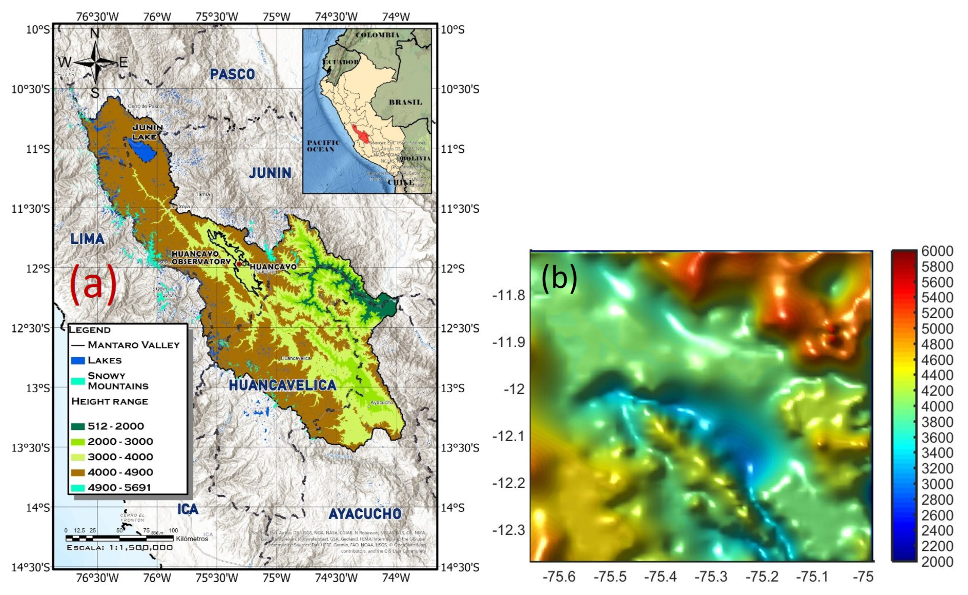
2. Site and Location

The HYO is located inside the Mantaro valley (MV) which is a part of the Mantaro river Basin (MRB) with a drainage area of 34,550 km 2 and placed in the central Andes of Peru (10.6 ° S–13.6 ° S; 73.9 ° W– 76.7 ° W). The MRB covers some territories of the Ayacucho, Huancavelica, Pasco, and Junin regions. The Peruvian central Andes has altitudes of 500–5350 m above sea level (m asl), with an average altitude of 3870 m asl (Figure 1). On the MRB, almost 83% of the annual rainfall occurred during the rainy season (September to March) and the rest (17%) occurred in the dry season (April to August). Along the MRB, it was estimated that the average of the annual precipitation is lower than 1600 mm year 1 , with the highest accumulation rainfall observed on the eastern part of the basin and the lowest over the central and southern regions of the MRB. During the dry season, rainfall is only significant in the eastern area of the basin due to the warm and moist fluxes from the Amazon basin [16].
Moreover, on the MRB, the maximum air temperatures have a less pronounced seasonality; meanwhile, the highest mean value was observed in November (20.8 ° C) and the lowest from February to March (18.4 ° C). In contrast, the minimum air temperatures have a more significant seasonality, ranging from its lowest mean values during the dry season (around 0.5 ° C), and highest mean values in the rainy season (around 7.0 ° C) [17]. The lowest values of the minimum mean temperature on the HYO were associated with cloudless conditions and large outgoing long-wave radiation, mainly during the dry season. The seasonal pattern of the frost events is associated with low cloud cover and low specific humidity, with minimum values in June and July at 07 LT. For specific humidity, diurnal variation is less pronounced with the minimum as close to 5.0 g kg 1 at 07 LT in the dry months and maximum values around 9.0 g kg 1 at 13 LT between January and March [12].
On the other hand, using a sun-photometer, the background conditions of aerosol optical detph (AOD) generally prevail in the HYO, with mean values around 0.10 ± 0.07. The analysis of monthly means reveals that September is the month with the highest AOD values, followed by August, October, and July. These background conditions are dominated, firstly, by continental aerosols with 67.1% of all the measured aerosols, followed by urban-industrial aerosols with 10.1% and, to a lesser extent, maritime aerosols (4%). The period associated with the increase in registered AOD in the HYO covers from July through October of each year and considers September as the month of the maxima. During these months, the background conditions are disrupted by the presence of biomass-burning aerosols, coinciding with the greater occurrence of forest fires, mainly in Peru, Bolivia, and Brazil. The biomass aerosols are the main party responsible for the increase of AOD in the Mantaro Valley and take the second place in all aerosols registered in HYO (18.2%) [15].

3. Methodology

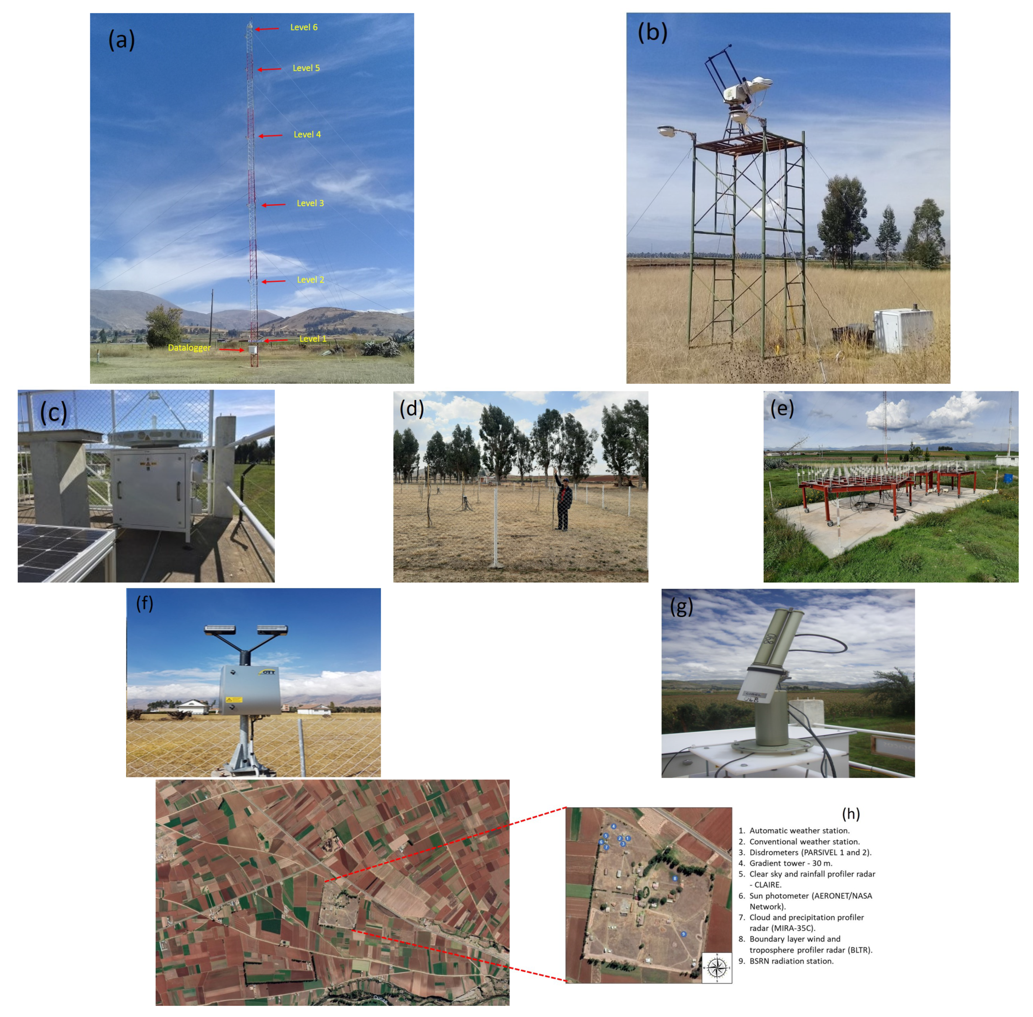
3.1. Instrumentation

3.1.1. Radars and Sensors

With the aim to obtain atmospheric data to study the physical processes associated with the occurrence of extreme meteorological events, the Geophysical Institute of Peru implemented the Laboratory of Physics, Microphysics and Radiation (LAMAR) in 2015 at the HYO (12.08 ° S, 75.38 ° W, 3313 m asl). LAMAR is composed of a set of different instruments and sensors that can be used for atmospheric studies and validation of numerical models in the Peruvian central Andes. The location of LAMAR’s instruments inside the HYO is shown in Figure 2h.
The set of the instruments is made up of: a Ka-band cloud and precipitation profiler radar (MIRA-35C); a VHF BLTR; a disdrometer second-generation particle, size and velocity (PARSIVEL 2), and some rain gauges pluviometers. Moreover, the new UHF wind profiles called Clear-Air and Rainfall Estimation radar (CLAIRE) was installed, which was fully designed and constructed at IGP’s technological development facility, the Jicamarca Radio Observatory (JRO) [18]. The main characteristics of all radars can be observed in Table 1. More information about inter-comparison between BLTR, CLAIRE and MIRA-35C can be found in [19].
LAMAR also has a set of sensors to measure meteorological variables of air and soil (temperature, relative humidity, wind speed, and wind direction) that were installed in a 30-meter-high gradient tower. To measure temperature and relative humidity, HMP60 probe of Campbell Scientific was used. Wind speeds and directions were measured using 03002Wind Sentry Set of Campbell Scientific that consists of a 3-cup anemometer and a wind vane mounted on a small cross-arm. The set also has a HFP01 soil heat flux plate that sends out a voltage signal proportional to the heat flux of the surrounding medium (soil).
Moreover, to measure the soil temperature and moisture, a set of Decagon 5TM VWC tensiometers was used. The 5TM delivered temperature and volumetric water content, which are measured by an on-board thermistor. It can also determine volumetric water content (VWC) by measuring the dielectric constant of the soil using capacitance/frequency- domain technology. All details of these sensors have been mentioned in Table 2.
Additionally, in order to measure the hemispherical (global and diffuse) SW irradiance, three pyranometers CMP10 (Kipp & Zonen) installed in the radiation tower were used (Figure 2b). Two of them measured the SW global and diffuse irradiances incident at the surface, and the other measured the SW irradiance reflected by the surface. A small black sphere mounted on an articulated, shading assembly in a two-axis automatic sun tracker 2AP (Kipp & Zonen) was used to measure the diffuse irradiance from the sky by blocking the direct solar irradiance (Figure 2b), and a pyrheliometer CHP1 (Kipp & Zonen), was used to measure direct SW irradiance. Finally, two pirgeometers CGR4 (Kipp & Zonen) installed in the radiation tower were used to measure LW irradiance incident and emitted by the surface. The main characteristics of these radiometers can be observed in Table 3.
Finally, on 19 March, 2015, as part of the AERONET network, a sun-photometer CIMEL CE-318T for aerosol measurement in the HYO was installed. (Figure 2g). This is the only instrument used for ground-based detection point for aerosol measurements in Peru. The CIMEL CE-318T uses eight spectral bands for solar and sky irradiance measurements (340, 380, 440, 500, 675, 870, 1020, and 1640 nm). Direct sun measurement (sun scenario) is the common procedure of the sun-photometer for aerosol measurements using a sample frequency of 15 min, which can help retrieve the spectral AOD and the Angström Exponent. On the other hand, the almucantar and principal plane scenarios are used for the sky irradiance measurements from which various aerosol properties are retrieved using inversion methods such as aerosol sizes distribution, single scattering albedo, and extinction coefficient [15]. The agricultural area of the study and location of all instruments in the HYO are shown in Figure 2h.

3.1.2. Global Precipitation Measurement (GPM), Global Forecast System (GFS) and MODIS Data

The GPM mission was built on the base of the Tropical Rainfall Measuring Mission (TRMM), which is a joint space mission between NASA and JAXA designed to monitor and study tropical and subtropical precipitation and associated release of energy. The GPM-IMERG products provide a greater coverage between 65 ° N and 65 ° S and generate global rainfall estimations every 30 min at 0.1 ° resolution. Furthermore, the GPM-IMERG products have shown improvements against rainfall gauges in comparison with another satellite-based precipitation products (TRMM-TMPA), under different climatic and topographic conditions located in China, Iran, United States, Tibetan plateau and slopes of the subtropical Andes [20,21,22,23,24,25,26,27]. A study over a 17-month period from April 2014 to August 2015 in Ecuador and Peru showed that GPM-IMERG has a superior detection and quantitative rainfall intensity estimation ability than TMPA, against a network of rain gauges, particularly in the high Andes [28]. For the present study, we used GPM-IMERG precipitation estimations to identify some intense rainfall events on the HYO.
Moreover, the GFS is a weather forecast model generated by the National Centers for Environmental Prediction (NCEP). The dataset of GFS contains several atmospheric and land-soil variables from atmospheric ozone concentration and soil moisture to precipitation, winds, and temperatures. The GPS products are used by the operational forecasters who predict weather about 16 days ahead because it covers the entire planet at a base horizontal resolution of 28 km between grid points. Finally, the MODIS instrument is a sensor on board of Terra and Aqua satellites. Its detectors measure 36 spectral bands between 0.405 and 14.385 m. It acquires data at three spatial resolutions: 250 m, 500 m, and 1000 m. Finally, the MODIS Cloud Product combines infrared and visible techniques to determine both physical and radiative cloud properties. The MODIS Cloud Product includes the cirrus reflectance in the visible spectrum at the 1-kilometer-pixel resolution, which is useful for removing cirrus scattering effects from the land-surface reflectance product. There are two MODIS Cloud data product files: MOD06_L2, containing the data collected from the Terra platform; MYD06_L2, containing the data collected from the Aqua platform.

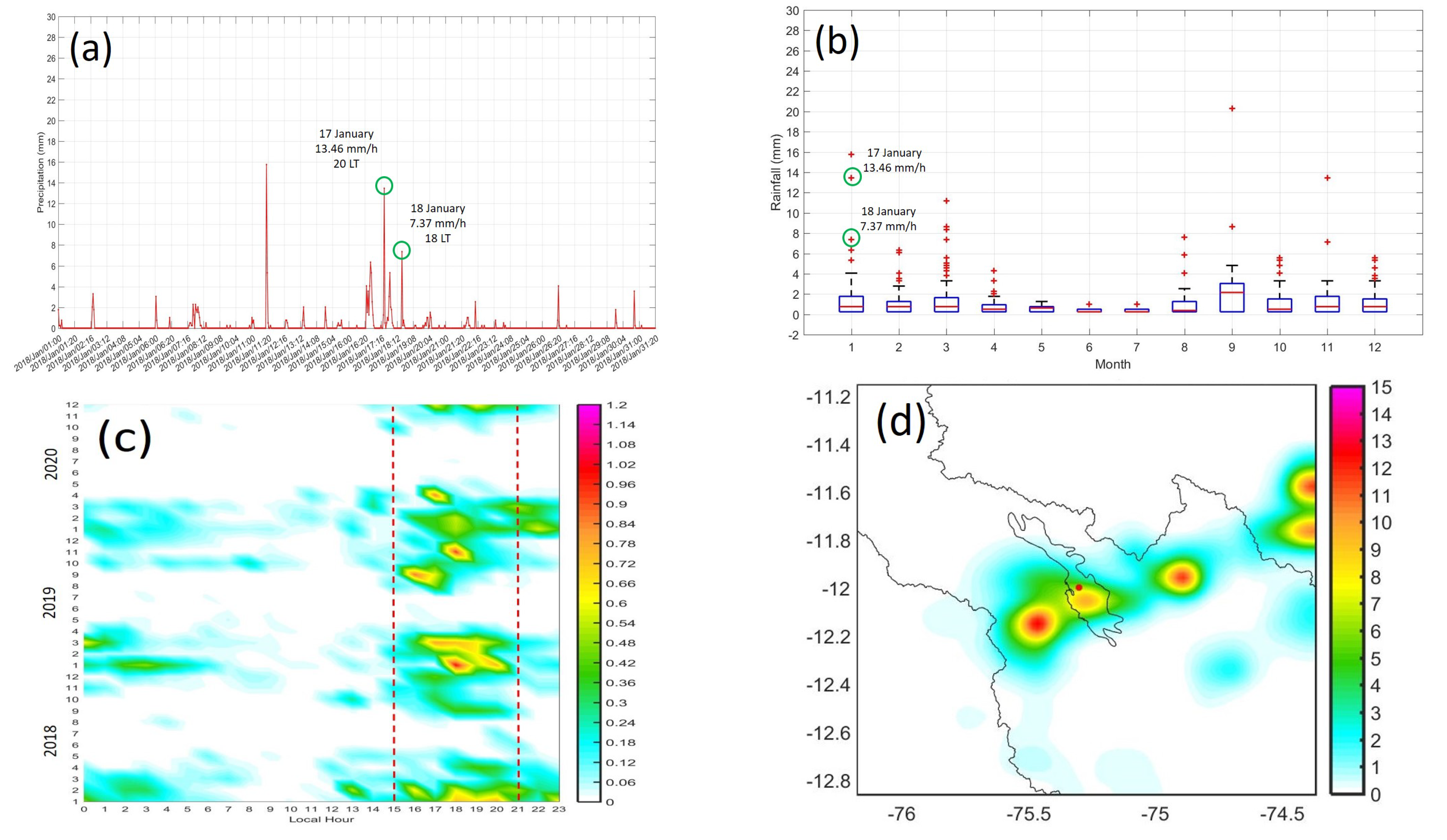
3.2. Identification of Extreme Events

To identify extreme rainfall events, we used boxplot and whiskers diagrams of accumulated hourly rainfall (mm h 1 ) for each month during 2018 and 2019. In addition, we used monthly climatological (1965–2019) mean, standard deviation, 90th percentile and maximum of daily accumulated rainfall (mm day 1 ). The two intense rainfall events, analyzed here, are hourly rainfall outliers of boxplot diagrams for January 2018 and December 2019, respectively. Moreover, both rainfall events have hourly rainfall values between standard deviation and 90th percentile of climatological daily accumulated rainfall.
A similar procedure was used to identify frost events. The boxplot and whiskers diagrams of hourly minimum temperatures ( ° C) for each month between July 2018 and July 2019, allow us to identify the minimum temperatures. Even more, we used monthly climatological (1965–2019) mean, standard deviation, 10th percentile and minimum values of daily minimum temperatures. The two frost events, analyzed here, are inside the minimum whiskers of boxplot diagrams of hourly minimum temperatures during June 2018 and April 2019, respectively. In addition, both frost events have minimum temperatures between 10th percentile and minimum of climatological daily air temperatures. In general, the occurrence of frost events can be analyzed in terms of the energy budget of the surface. The nocturnal cooling, which generates frost events at early morning hours, is mainly driven by the net long-wave radiation loss. However, the other energy budget components, such as heat and latent turbulent energy fluxes and heat flux transmitted to the ground, are also important to characterize the frost events and their estimations are shown in Section 3.3.
In relation to the high pollution events analyzed here, we selected them considering values of aerosol optical depth (AOD), estimated by the sun-photometer CIMEL CE-318T type, much higher than the mean value plus standard deviation of AOD equal to 0.10 ± 0.07 for the period from March 2015 to August 2017. The three high pollution events identified for the present study occurred between 6 and 10 August, 17 to 22 August and 29 August to 2 September 2019 on the HYO.

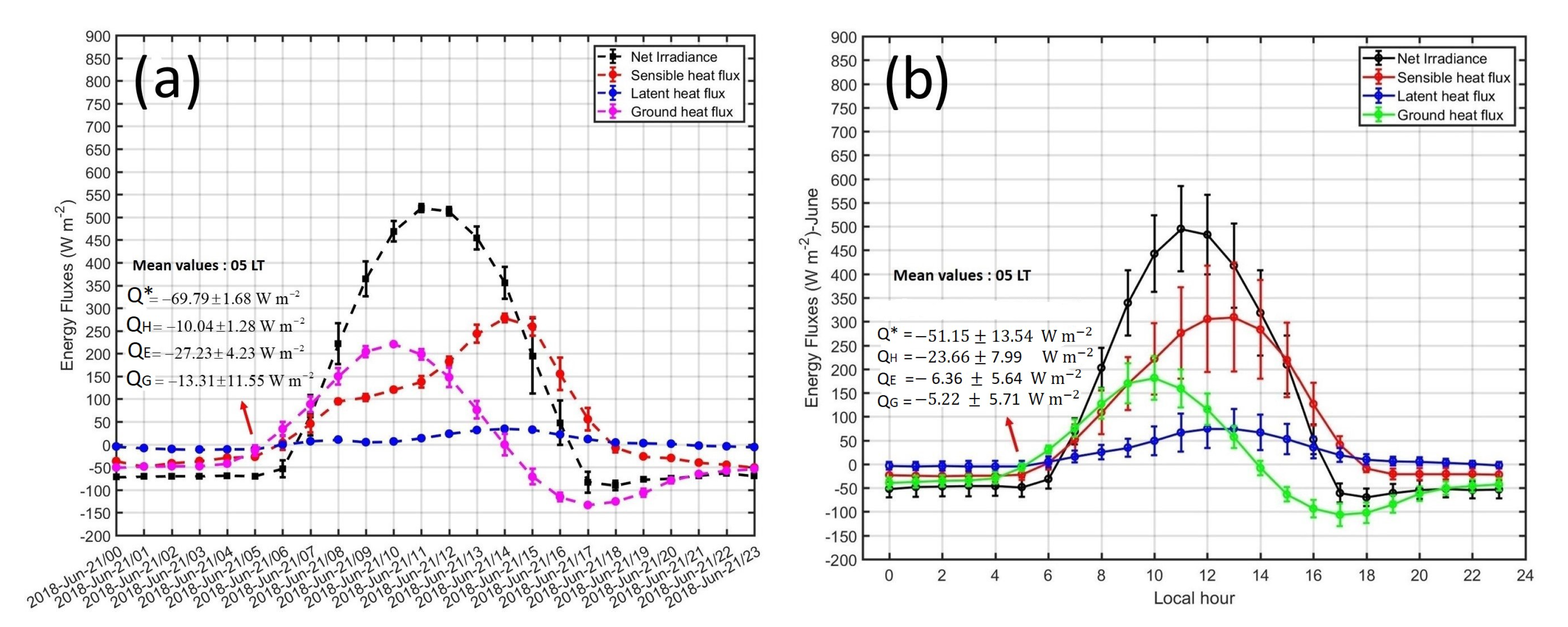
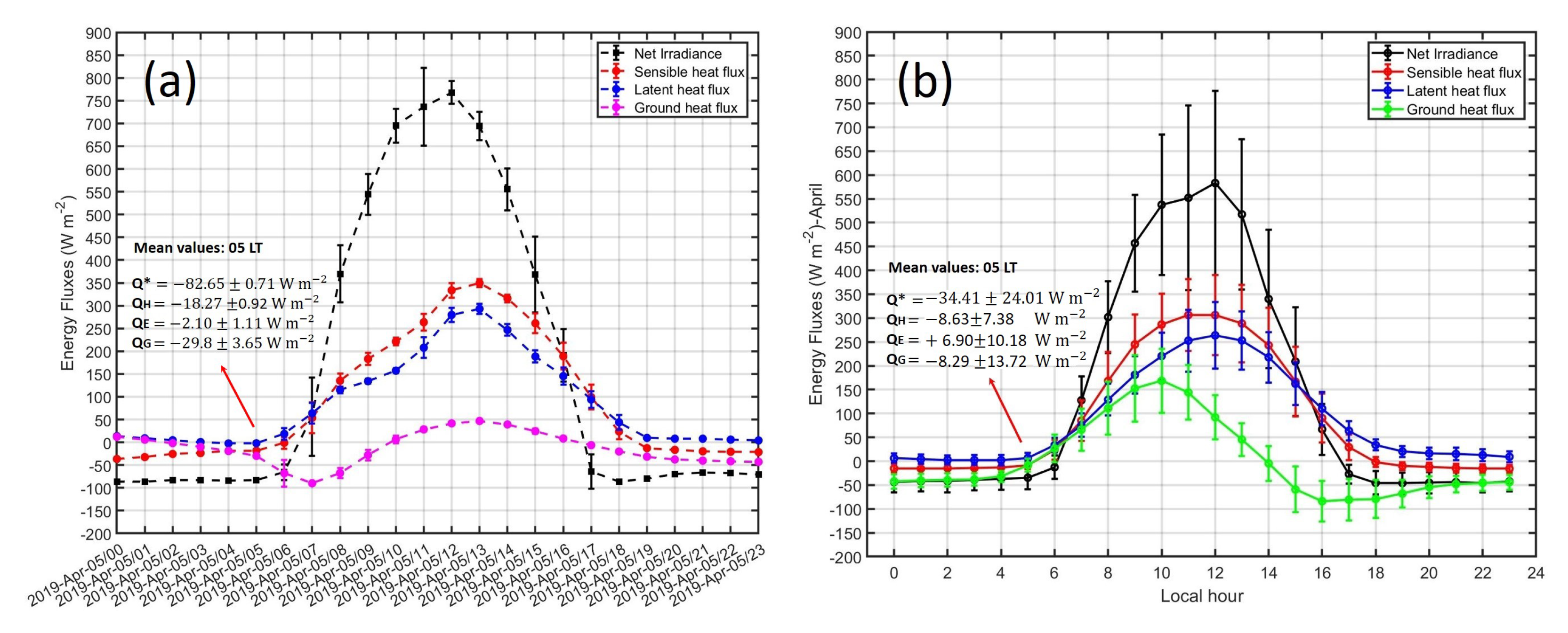
3.3. Estimation of Energy Balance Components

To estimate the turbulent energy fluxes (sensible and latent), we used the aerodynamic flux–gradient method [29] based on average profiles of atmospheric variables and the degree of turbulent activity. The aerodynamic method uses measurements of air temperature, relative humidity, and wind speed and direction with sensors located in the gradient tower (Figure 2a) with six different levels, as described in Section 3.1.1. The method is based on the similarity principle proposed by Monin and Obukhov [30,31]. This principle supports the equivalence between the diffusion coefficients and the aerodynamic resistance for momentum, heat, water vapor and carbon dioxide. This condition means that a turbulent eddy can carry heat, vapor, and momentum with equal efficiency. Moreover, we used the Bulk Richardson number (Ri B ), which is a non-dimensional stability parameter, to characterize atmospheric stability and the turbulence state near the surface [32], as it is a ratio that accounts for the effects of buoyancy and mechanical forgings (free to forced convection) and is expressed as follows:
Ri B = g T ¯ . Δ T ¯ / Δ z ( Δ u ¯ / Δ z ) 2
Here, g (m s 2 ) is the acceleration due to gravity, T ¯ (K) is the mean temperature in the layer Δ z (m), and Δ T ¯ is the difference of the temperatures in the layer Δ z , Δ u ¯ is the difference of wind speed in the layer Δ z . For Equation (1), the change of wind direction in low levels was assumed to be very low and, therefore, could be ignored. For neutral stability conditions, which generally occurred in early morning and/or evening periods on cloudy days with strong winds, Ri B approaches toward zero (±0.01). Meanwhile, for stable conditions, which occurred during early morning, evening, or night periods and overcast days when temperatures near the surface are cooler than away from the surface, Ri B corresponds to positive values. Finally, negative values of Ri B indicate strong lapse rate (unstable) conditions where surface heating enhances buoyancy effects. During the diurnal cycle, the atmosphere presents dominant periods of stable and unstable conditions, with neutral conditions representing only a minor fraction of the total period. The neutral form of the aerodynamic equations to estimate the turbulent energy fluxes of momentum ( τ ), sensible ( Q H ) and latent ( Q E ), can be generalized according to the level of stability [32,33], as given by Ri B in the following operational equations:
Q H = C a k 2 z 2 Δ u ¯ Δ z . Δ T ¯ Δ z . ( Φ M Φ H ) 1
Q E = L v k 2 z 2 Δ u ¯ Δ z . Δ ρ ¯ v Δ z . ( Φ M Φ V ) 1
τ = ρ k 2 z 2 Δ u ¯ ln ( z 2 / z 1 ) 2 . ( Φ M 2 ) 1
In Equation (2), ρ v is the water vapor density, which was estimated using the relative humidity, saturation vapor pressure and air temperature. Moreover, C a is the heat capacity of air, L v is the latent heat of vaporization, k is the Von Karman’s constant (∼0.40), z is the log mean height (=( z 2 z 1 )/(ln( z 2 / z 1 )), and Φ M , Φ H , and Φ V are dimensionless stability functions for momentum, heat and water vapor, respectively, which can be expressed as the functions of the Richardson number [32], using the following equation:
Φ M 1 = ( 1 15 R i ) 1 / 4 for R i < 0 ( 1 5 R i ) for 0 < R i < 0.2 Φ X 1 = ( 1 15 R i ) 1 / 2 for R i < 0 ( 1 5 R i ) for 0 < R i < 0.2
Here, Φ X is the appropriate stability function for the property being transferred. Using these functions, it is possible to calculate the combined terms used in Equation (2):
( Φ M Φ X ) 1 = ( 1 15 R i ) 3 / 4 for R i < 0 ( 1 5 R i ) 2 for 0 < R i < 0.2
For neutral conditions of the atmosphere (Ri between ±0.01), only forced convection is significant in comparison to thermal effects. For stable atmospheric conditions (Ri around to +0.25) vertical mixing is absent and the flow is laminar. In contrast, for conditions of higher instability (Ri larger higher than −1.0) there are weak horizontal motion and strong convective instability because buoyancy effects grow in importance through the mixed regime.

3.4. Ground Heat Flux at the Surface

The ground surface and the canopy are heated by the incoming short-wave irradiance during diurnal hours. Meanwhile, during night hours, the emission of long-wave up-welling irradiance leads to the cooling of the surface, which becomes cooler than the air above and the deeper soil layers. In general, the available energy, supplied by the net all- wave irradiance (Q * ) is distributed by the turbulent sensible (Q H ) and latent (Q E ) heat fluxes and the mainly molecular ground heat flux (Q G ), which is based mainly on molecular heat transfer and is proportional to the soil temperature gradient ( T / z ) multiplied by the thermal molecular conductivity a G (W m 1 K 1 ). To estimate the ground heat flux at the surface, we used the sum of the soil heat flux measured at 8 cm, by a soil heat flux plate and the heat storage in the layer between the surface and the plate [34]:
Q G ( 0 ) = Q G ( 8 c m ) + z 0 C G ( z ) T ( z ) d z
Here, C G is the volumetric heat capacity, C G (z) = a G / ν T ( ν T is the molecular thermal diffusivity) that can be assumed constant with depth in the case of uniform soil moisture. To implement Equation (7), we used two integrating temperature sensors of the soil layer, located at a distance of 2 cm and 5 cm between the surface and the heat flux plate (8.0 cm). For the ground heat flux near the surface, it follows the equation given below:
Q G ( 0 ) = Q G ( 8 c m ) + C G | Δ z | | T ( t 2 ) T ( t 1 ) | t 2 t 1
In addition, C G values of moist soil at different soil levels were calculated by adding the heat capacity of the dry soil to that of the soil water, as represented by the following equation:
C G = C d + θ V ρ W C W
Here, C d is the heat capacity of dry soil, θ V is the soil water content on a volume basis, ρ W is the density of water (1000 kg m 3 ), and C W is the specific heat of water (4.18 × 10 3 J kg 1 K 1 ). A value of 1.25 × 10 6 J m 3 K 1 for the heat capacity of dry soil is reasonable for clay soil according to the soil characteristics of the HYO [35]. Section 4 shows the analysis of the main results of the present study.

4. Analysis of the Results

4.1. Intense Rainfall Events

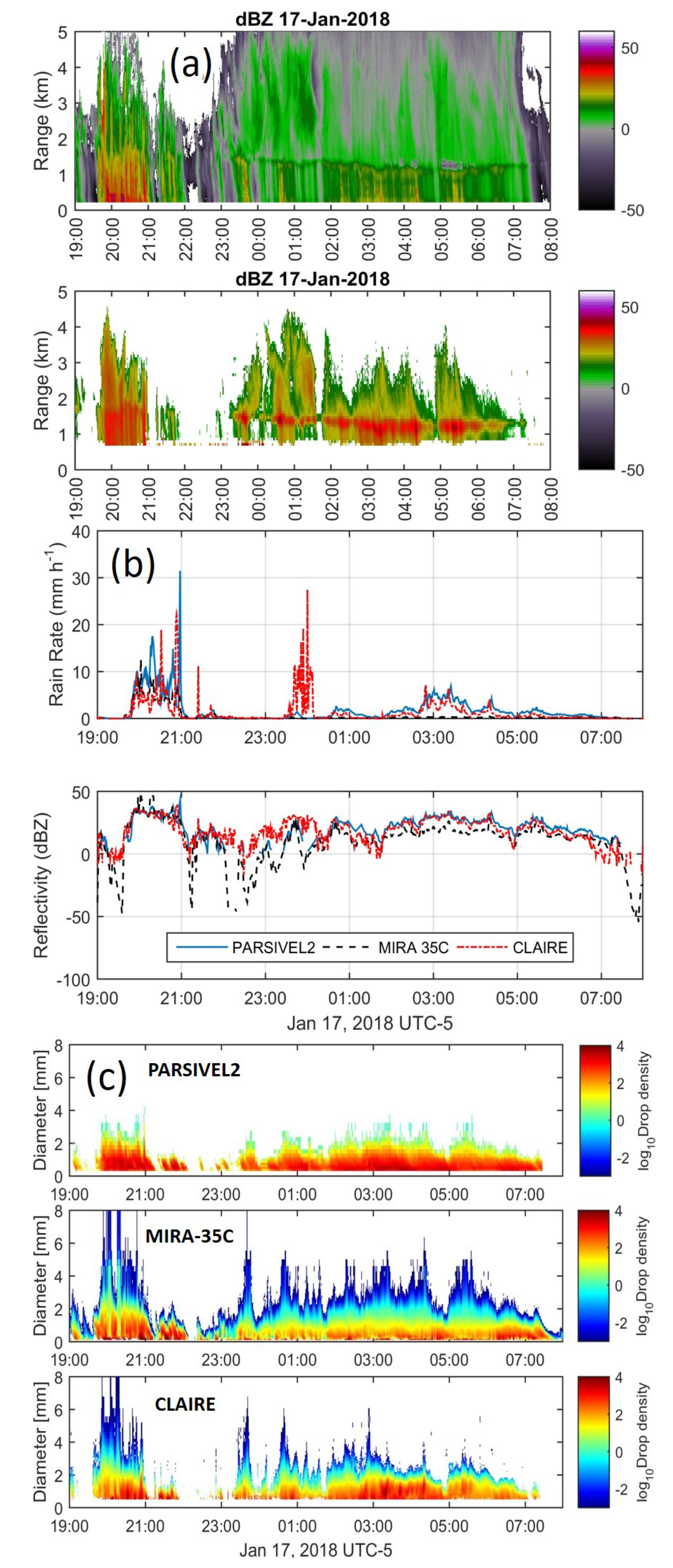
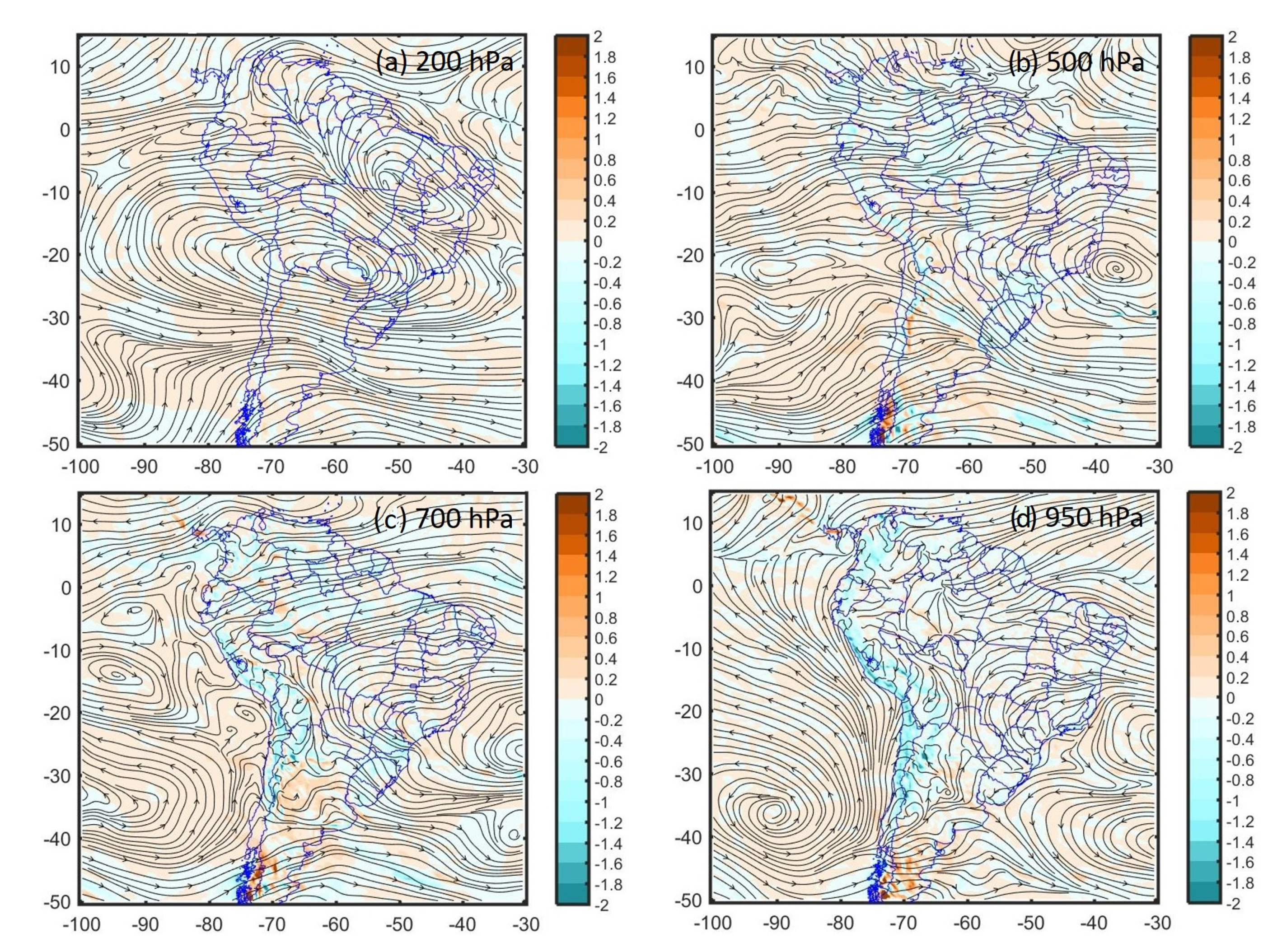
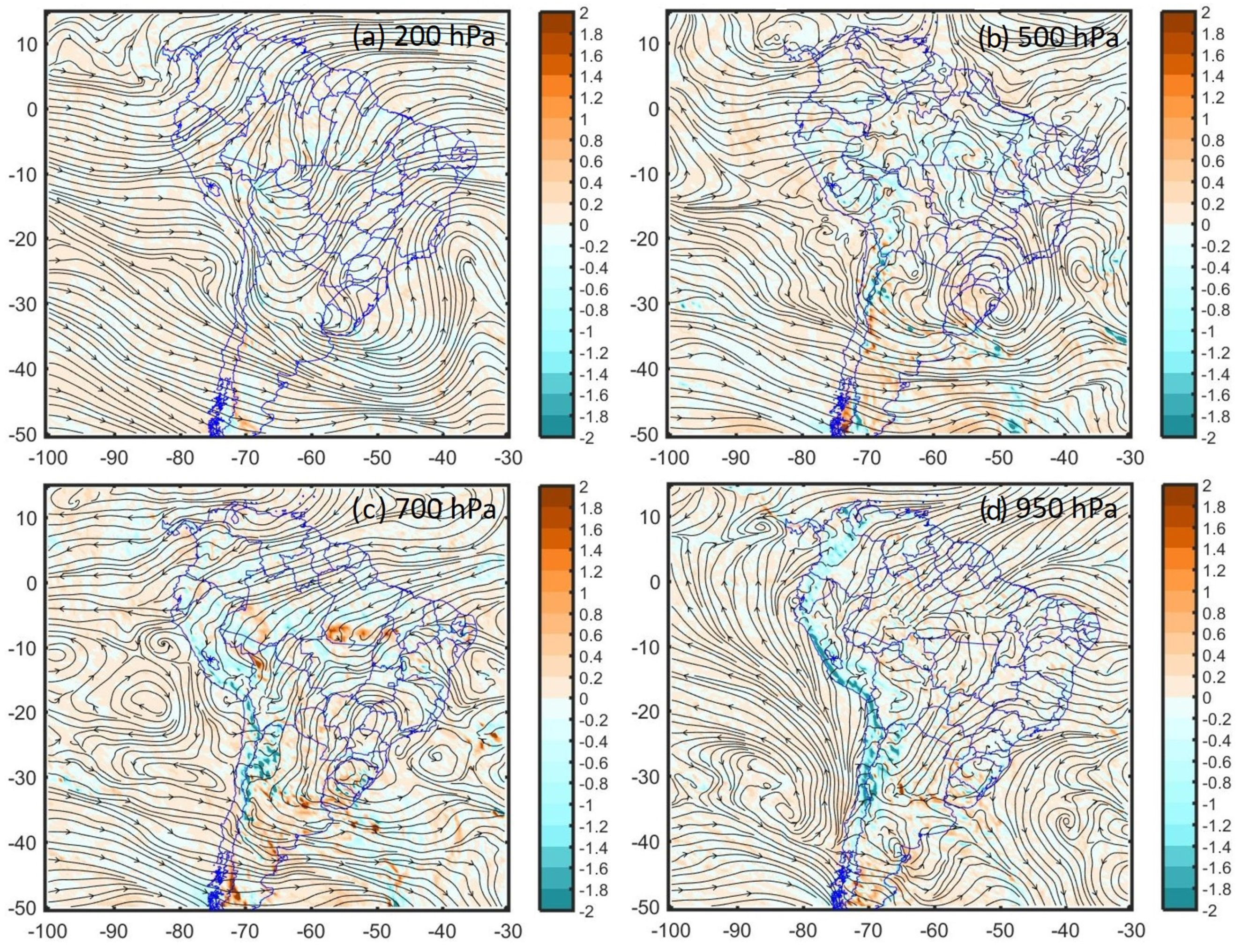
4.1.1. Event on 17 January 2018

The time series of the accumulated hourly rainfall rate (mm h 1 ) measured by in-situ pluviometers above the HYO during January 2018 is shown in Figure 3a. A total of three events with high rainfall rate were observed: the first one occurred on 11 January at 19 LT with a peak of 15.75 mm h 1 , the second on 17 January at 20 LT with a peak of 13.46 mm h 1 , and the third on 18 January at 18 LT with a peak of 7.37 mm h 1 . It is important to note that the last two events occurred on two consecutive days, and for those days, weaker precipitation during the night hours was observed. These rainfall events were extremes in the sense of that the hourly accumulated rainfall are higher than the mean values plus the standard deviations in a boxplot and whiskers diagrams, as shown in Figure 3b. It was observed that during January 2018, the events mentioned above were two of the higher outliers with a rainfall median close to 1 mm h 1 and a maximum close to 4 mm h 1 .
In addition, the maximum rainfall peak on 17 January (13.46 mm h 1 ) was lower than the maximum climatological (1965–2019) daily accumulated rainfall, as shown in Figure 6d, with maximum values close to 42 mm day 1 in January, and approximately equal to the climatological percentile 90% (14 mm day 1 ) for the same month. Monthly and diurnal cycles of mean hourly accumulate rainfall during 2017, 2018, and 2019 are shown in Figure 3c. It is important to note that the highest amount of rainfall occurred between August and March at 15 LT and 21 LT for all years. Particularly, during 2018, the highest mean hourly rainfall occurred in January at around 18 LT. The spatial distribution of rainfall rate estimated by GPM system for 17 January 2018 at 21 LT is shown in Figure 3d. Four areas of high precipitation rate that aligned from north-east to south-west with a core of 7 mm h 1 above the HYO were observed.
Moreover, the reflectivity factor in function of time and altitude estimated by radar MIRA-35C and radar CLAIRE above the HYO on 17 January 2018 are shown in Figure 4a,b, respectively. Note that the range closest to the surface from which the radars begin to be measured are 250 m for MIRA-35C and 750 m for CLAIRE. Both radars identified high values of reflectivity close to 40 dBZ between 20 LT and 21 LT. However, the reflectivity data from MIRA-35C, working at 35 GHz ( λ = 8.6 mm), was usually more attenuated than that from CLAIRE that works at 445 MHz ( λ = 670 mm). Moreover, it was observed that the data from MIRA-35C was degraded by clouds and precipitation, in comparison with the data from CLAIRE, with the attenuation being higher when the radar beam flows through a large number of hydrometeors from the surface up to a high of approximately 4 km high. This attenuation was also found to be between 23 LT and 0730 LT when observed on the HYO for the stratiform precipitation. The MIRA-35C radar determined maximum reflectivity values to be between 20 dBZ and 30 dBZ. Meanwhile, CLAIRE radar measured maximum values between 30 dBZ and 40 dBZ as its attenuation effects are negligible due to its lower operating frequency (445 MHz).
In addition, Figure 4b shows the time series of rain rate (mm h 1 ) and reflectivity (dBZ) measured by PARSIVEL2, MIRA-35C, and CLAIRE at their lowest level of measurement. It is important to note that the rain rate reaches close to 30 mm h 1 around 21 LT at its minimum level (2 m). Meanwhile, for MIRA-35C and CLAIRE, the rain rates are lower, with values between 10 mm h 1 and 20 mm h 1 , which is probably due to their higher minimum level of measurement, which is 250 m for MIRA-35C and 750 m for CLAIRE. However, around 00 LT, CLAIRE radar measured high rain rate with maximum values between 20 mm h 1 and 30 mm h 1 , which indicated the presence of hydrometeors at 750 m; however, MIRA-35 and PARSIVEL2 are able to observe almost nothing at 250 m and 750 m. This situation revealed that the concentration of hydrometeors is highly dependent on height and time during a convective process occurring above the HYO. A similar behavior was observed for the reflectivity values measured by all the devices. Moreover, the drop size distribution retrieval by MIRA-35C, CLAIRE and PARSIVEL2 are shown in Figure 4c. It was observed that PARSIVEL2 measured a high concentration of hydrometeors with sizes between 0.2 and 2 mm and some hydrometeors of sizes around 3 mm. On the contrary, MIRA-35C and CLAIRE observe a wide variety of hydrometeor sizes, with values up to 8 mm due to their higher observation rate.
The mean synoptic conditions obtained from the GFS reanalysis data for the event on 17 January, 2018, at 13 LT are shown in Figure 5. At high levels (200 hPa: Figure 5a) of the atmosphere, the event is characterized by the presence of the centered BH-NL system, approximately at 22 S and 60 W, which generates strong easterly circulations at latitudes around the MV between 5 S and 20 S. At mid levels of the atmosphere (500 hPa: Figure 5c and 700 hPa: Figure 5d), strong easterly circulations around the Mantaro valley were also observed, on the east side of the Andes cordillera, which is probably associated with the intensification of south-easterly trade winds. At low levels of the atmosphere (950 hPa: Figure 5d), strong north-westerly thermal circulations were observed along the east side of the Andes in association with the South America Low Level Jet (SALLJ) that intrude into the higher altitudes of the Andes. Meanwhile, at the west side of the Andes, strong south-easterly circulations coming from the Pacific Ocean were observed that intrude into the continent, generating strong ascending vertical velocities with values around −1.2 Pa s 1 . This atmospheric configuration showed that during the occurrence of the events on 17 and 18 January 2018, the patterns of easterly circulation events in the central Andes of Peru prevailed, as identified in [10].

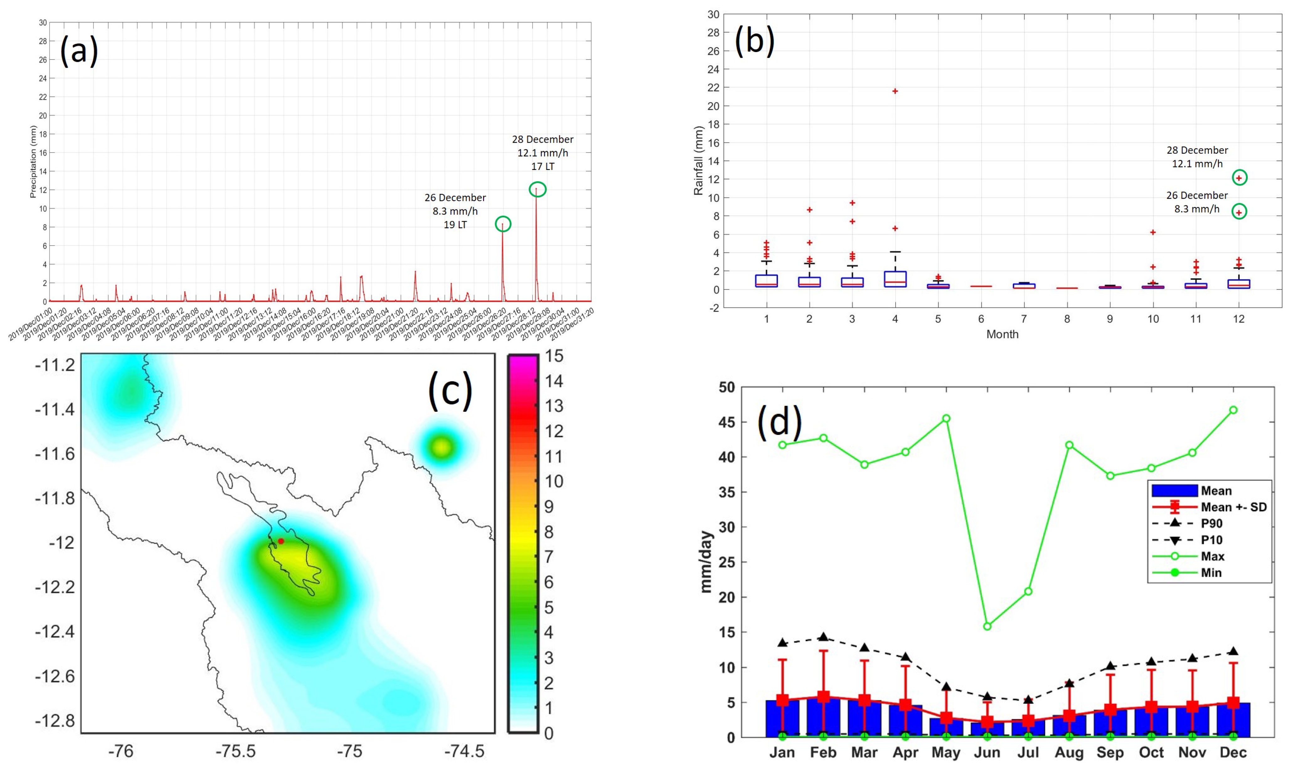
4.1.2. Event on 28 December 2019

The time series of the accumulated hourly rainfall rate (mm h 1 ) measured by in situ pluviometers above the HYO during December 2019 is shown in Figure 6a. Two events with high rainfall rates were observed: the first one occurred on 26 December at 19 LT with a peak of 8.3 mm h 1 and the second on 28 December at 17 LT with a peak of 12.1 mm h 1 . It was observed that these two events lasted for only two hours and occurred on with only one day of separation. As in the previous case, these rainfall events are extreme in the sense of that they are outliers in a boxplot and whiskers diagrams, which are shown in Figure 3b. It was observed that during December 2019, the events mentioned above are the higher outliers with a rainfall median close to 0.5 mm h 1 and a maximum value close to 2.1 mm h 1 .
In addition, the maximum rainfall peak on 28 December (12.1 mm h 1 ) was lower than the maximum climatological (1965–2020) daily accumulated rainfall, as shown in Figure 6d, which has maximum values close to 47 mm h 1 in December, and close to the climatological percentile 90% (13 mm day 1 ) for the same month. Furthermore, the spatial distribution of rainfall rate estimated by GPM system for 28 December 2019 at 18 LT is shown in Figure 6c. In contrast to the event on 17 January 2018, two areas of high precipitation rate aligned from north-west to south-east with a core of 7 mm h 1 above the HYO were observed.
The mean synoptic conditions obtained from the GFS reanalysis data for the event on 28 December 2018 at 13 LT are shown in Figure 7. In contrast to the event on 17 January 2018, at high levels (200 hPa: Figure 7a) of the atmosphere, this event was characterized by the absence of the BH-NL system and presence of strong westerly circulations around the location of the MV. However, at the level of 500 hPa (Figure 7c), a small anticyclonic system that generates easterly circulations around the location of the MV was observed. Similarly, at the level of 700 hPa: (Figure 7d), easterly circulations at the east side of the Andes cordillera, associated with the intensification of trade winds, were also observed. At low levels of the atmosphere (950 hPa: Figure 7d), strong north-westerly circulations along the east side of the Andes, associated with the SALLJ that intrude into the higher altitudes into the Andes, were observed. Meanwhile, at the west side of the Andes, it was observed that there were strong south-easterly circulations coming from the Pacific Ocean that intrudes into the continent, generating strong ascending vertical velocities with values around −1.8 Pa s 1 , which are higher than the values for the event on 17 January, 2018. This atmospheric configuration showed that during the events on 17 and 18 January 2018, there prevailed easterly circulations in the central Andes of Peru, as was identified in [10]. This atmospheric configuration also showed that during the occurrence of events on 26 and 28 December 2019, there prevailed patterns of westerly circulation in the central Andes of Peru, as identified in [10].

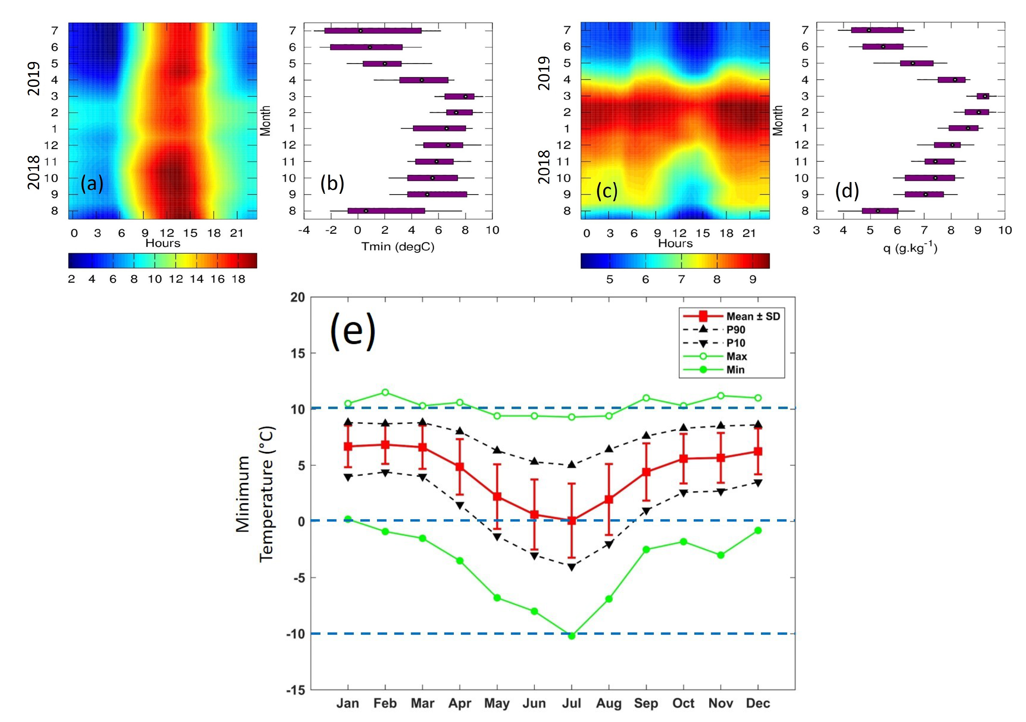
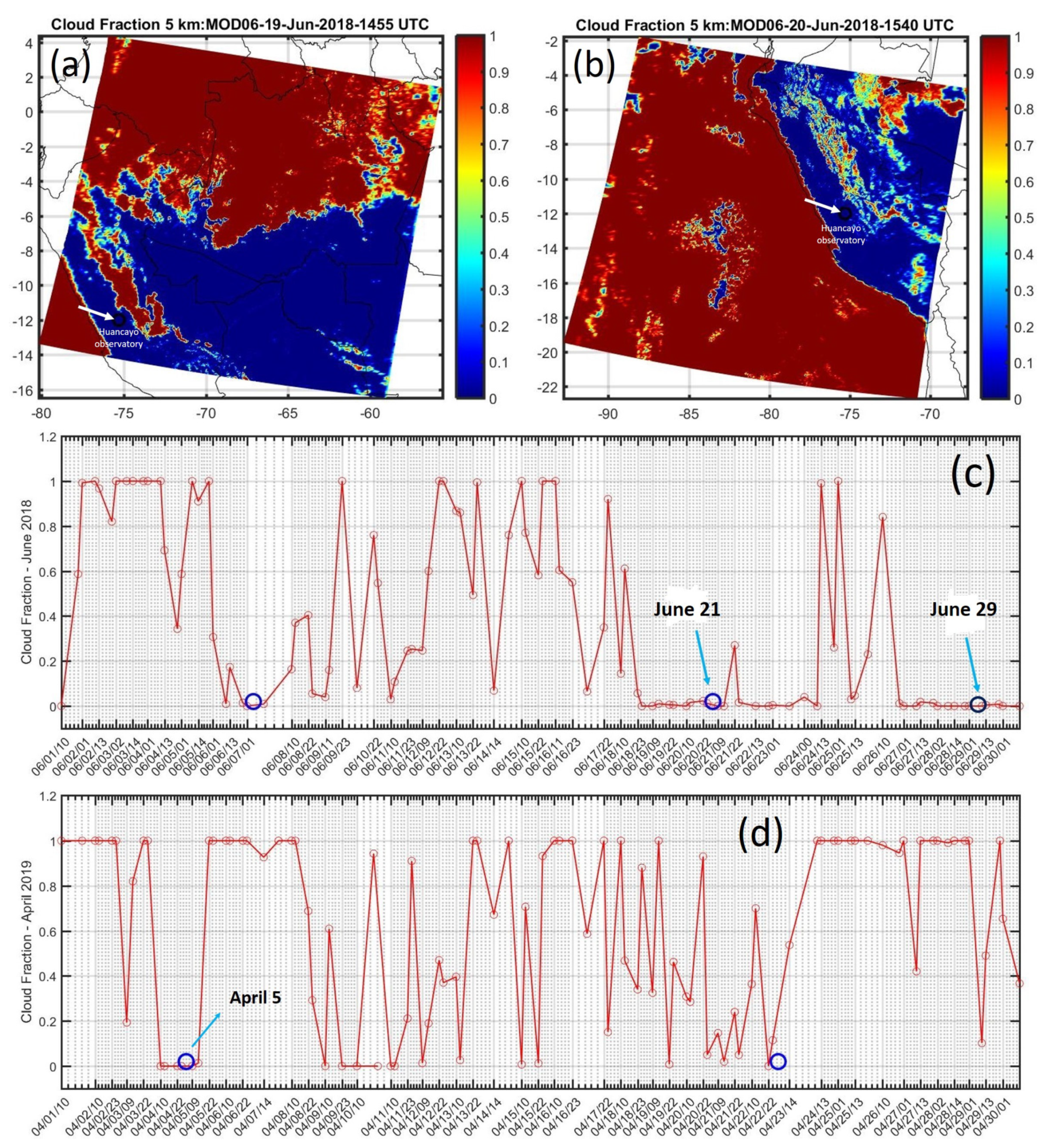
4.2. Intense Frost Events

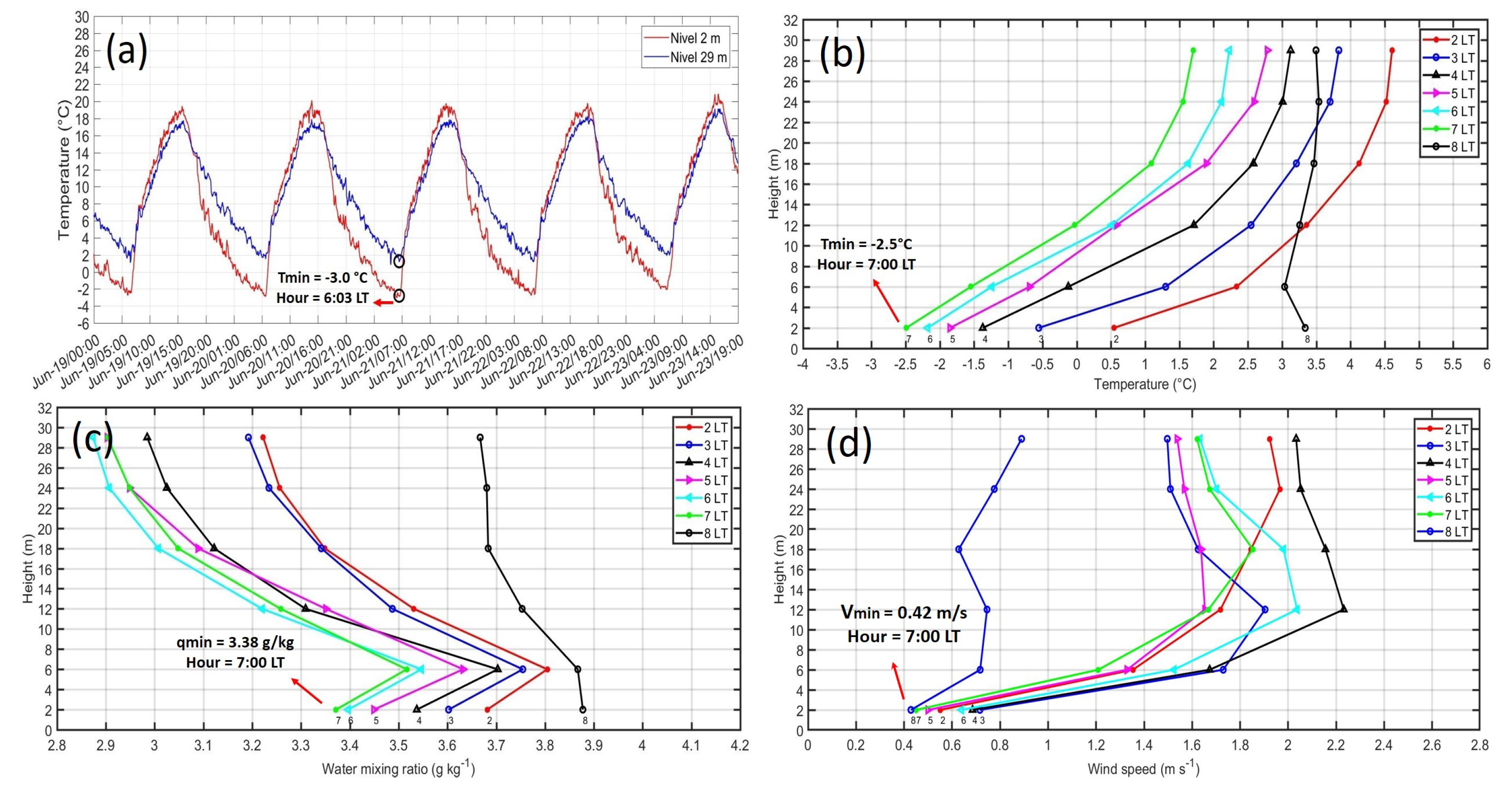
4.2.1. Event on 21 June 2019

In this section, we analyzed the intense frost event on 21 June 2019 above the HYO. Time series of air temperature at heights of 2 m and 29 m between 19 and 23 June, 2018, are shown in Figure 8a. The minimum temperatures reached nearly −3.0 C at a height of 2 m and +2 C at 29 m high at around 0603 LT on 21 June 2018. This frost event was identified as extreme because the minimum temperature at 2 m was close to the lower values of mean hourly minimum temperatures during June 2019, as shown in the boxplot diagram in Figure 9b. Moreover, this value (−3.0 C) was close to the climatological (1965–2019) percentile 10% of minimum temperatures, as shown in Figure 9e. However, the minimum climatological temperature reached about -8 C above the HYO during June.
Moreover, the monthly and diurnal cycles of mean hourly temperatures at a height of 2 m above the HYO between July 2017 and July 2018 are shown in Figure 9a. In general, maximum mean hourly temperatures were observed between September and November at around 12 LT and 15 LT with values close to +18 C. Meanwhile, minimum mean hourly temperatures were observed during April and July between 00 LT and 07 LT with values of around +2 C. Furthermore, the variations of monthly minimum temperatures quantiles (boxplot) are shown in Figure 9b. The minimum values of monthly minimum temperatures were observed in June, July, and August with values between −2.0 C and −4 C.
It is important to note the continuous decrease (increase) of minimum temperatures during the days preceding (following) the occurrence of this extreme frost event. Moreover, Figure 8b shows the mean hourly temperature vertical profiles between 02 LT and 08 LT for the event on 21 June 2018 above the HYO. At night hours, very stable conditions of the surface boundary layer, with positive lapse rates close to 0.27 C m 1 and minimum temperatures close to −2.5 C at 07 LT, were observed.
Mean hourly vertical profiles of water vapor mixing ratio between 02 LT and 08 LT of 21 June 2018 above the HYO are shown in Figure 8c. It is important to note that the water vapor vertical profiles become inverted near the surface (below 6 m) during night hours reached a positive lapse rates around +0.038 g kg 1 m 1 and minimum values of water vapor mixing ratios at a height of 2 m close to 3.35 g kg 1 at 07 LT. Moreover, the mean hourly wind speed vertical profiles between 02 LT and 08 LT of 21 June 2018 above the HYO are shown in Figure 8d. It is important to note the presence of a surface jet with maxima of 2.2 m s 1 at a height of 12 m at around 04 LT. This jet reached its maximum intensity around 04 LT and was probably associated with the katabatic wind of mountain-valley circulations inside the MV.
Moreover, the monthly and diurnal cycles of mean water vapor mixing ratio at a height of 2 m above the HYO between July 2017 and July 2018 are shown in Figure 9c. Maximum mean hourly water vapor mixing ratios with values close to 10 g kg 1 , were observed between January and March around 16 LT and 21 LT; meanwhile, minimum mean water vapor mixing ratio with values close to 5 g kg 1 were observed between May and August at around 00 and 07 LT, and 12 LT and 16 LT. We emphasized that these value of minimum temperature (−2.5 C) and minimum water vapor mixing ratio (3.3 g kg 1 ), which were registered during the extreme frost events on 21 June 2018, were lower than the mean monthly minimum values shown in boxplots and whiskers diagrams during June 2018, indicating minimum temperatures close to −3.0 C (Figure 9b) and minimum water vapor mixing ratios of around +4.5 g kg 1 (Figure 9d).
The spatial distribution of the cloud fraction products obtained by MODIS sensor (MOD06_L2 and MYD06_L2) onboard of Terra and Aqua satellites above the HYO on 19 January 2018 at 0955 LT and 20 January 2018 at 1040 LT are shown in Figure 10a and Figure 10b, respectively. For both times, clear sky conditions along the Andes cordillera including the HYO were observed. Figure 10c shows the time series of mean cloud fraction obtained from MODIS sensor around 10 km above the HYO during June 2018. It was observed that three days before the occurrence of the frost event on 21 June at 06 LT, the amount of cloud fraction above the HYO was almost zero, favoring the surface net-long wave radiation loss (L * ). Later, the cloud fraction increased slightly up to almost 0.3. Moreover, another period of three days with almost zero cloud fraction up to the occurrence of the next frost event on 29 June was also observed.
On the other hand, the daily cycle of mean hourly values and standard deviations of the energy balance components during the frost event on 21 June 2018 are shown in Figure 11a. During early morning hours (05 LT), the net irradiance (Q * ) had minimum values close to −69.8 W m 2 , the sensible heat flux (Q H ) showed minimum values of around −10.0 W m 2 , the latent heat flux (Q E ) showed minimum values of around −27.2 W m 2 , and finally, the ground heat flux (Q G ) presented minimum values close to −13.3 W m 2 . These mean hourly values of the energy balance components were significantly lower than those during June 2018, which are shown in Figure 11b, with the exception of Q H whose value is higher than the mean monthly value. During night hours, the mean monthly values of Q * showed minimum values close to −51.15 W m 2 , Q H showed minimum value close to −23.66 W m 2 , Q E showed a minimum value close to −6.36 W m 2 , and finally, Q G showed a minimum value of around −5.22 W m 2 . It is important to highlight that the imbalance term (Q * − Q H − Q E − Q G ) was equal to −19.21 W m 2 at 05 LT.
During diurnal hours on 21 June 2018, maximum Q * reached values close to 520.4 W m 2 around noon, which was higher than the mean monthly values in June (495.2 W m 2 around noon). In contrast, the standard deviation values of Q * were significantly lower than the mean monthly values, which was an indication of the prevalent clear sky conditions on 21 June. In contrast, maximum Q H was 278.1 W m 2 at around 14 LT, which was slightly lower than the mean monthly values of Q H in June (309.2 W m 2 at 14 LT). The same occurred for Q E with maximum values of 34.49 W m 2 at around 14 LT, which was lower than the mean monthly values of Q E in June (74.86 W m 2 ). Finally, maximum Q G value was 220.6 W m 2 at 10 LT, which was higher than the mean monthly values in June (181.5 W m 2 at 10 LT). In general, the standard deviations of all energy balance components on 21 June 2018 were significantly lower than the mean monthly values.

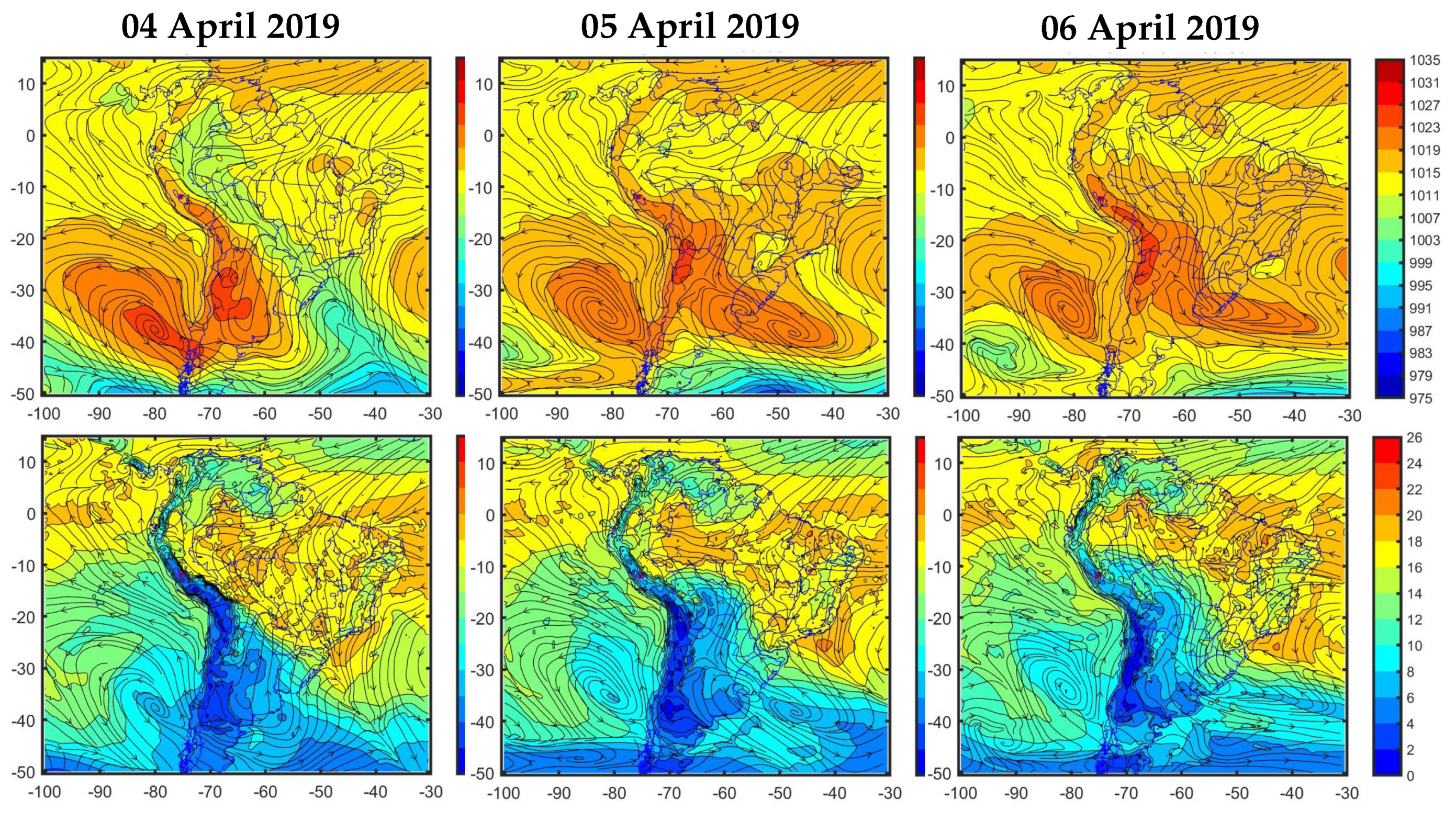
4.2.2. Event on 5 April 2019

In this section, we analyzed the intense frost event on 5 April 2019 above the HYO. Time series of air temperature at a height of 2 m and 29 m between 3 and 7 April 2019 are shown in Figure 12a. The minimum temperatures reached values close to +0.23 C at a height of 2 m and +6 C at a height of 24 m at around 0521 LT on 5 April 2019. In contrast to the previous frost event on 21 June 2018, the minimum temperature of the days before and after the occurrence of this frost event presented with higher temperatures close to 4 at a height of 2 m. However, as in the previous case, this frost event was identified as extreme as the minimum temperature at 2 m height was close to the lower values of mean hourly minimum temperatures during April 2019, as shown in the boxplot diagram in Figure 9b. Furthermore, this value (+0.23 C) was close to the climatological (1965–2019) percentile 10% of minimum temperatures (1.0 C), as shown in Figure 9e. However, the minimum climatological temperature reached above the HYO in June was about −4 C.
Moreover, Figure 12b shows the mean hourly temperature vertical profiles between 02 LT and 08 LT on 5 April 2018 above the HYO. At night hours, very stable conditions of the surface boundary layer with positive lapse rates higher than the previous frost event, with values close to +0.34 C m 1 , were observed. Moreover, it was also the minimum temperature was higher than the previous frost event, with values close to +0.30 C at 06 LT.
Mean hourly vertical profiles of water vapor-mixing ratio between 02 LT and 08 LT on 5 April 2019 above the HYO are shown in Figure 12c. As in the previous frost event, the water vapor vertical profiles become inverted near the surface (below 6 m) in night hours, reached lower positive lapse rates at around +0.011 g kg 1 m 1 and higher minimum values of water vapor mixing ratios at a height of 2 m close to 5.03 g kg 1 at 06 LT. Moreover, the mean hourly wind speed vertical profiles between 02 LT and 08 LT on 5 April 2019 above the HYO are shown in Figure 12d. As in the previous frost event, the presence of a surface jet with maximum of 2.33 m s 1 around 29 m at 02 LT was observed. This jet reached its maximum intensity at around 02 LT and was probably associated with the katabatic wind of mountain-valley circulations inside the MV.
As in the previous frost event on 21 June 2018, the value of minimum temperature (+0.23 C) and water vapor mixing ratio (+5.03 g kg 1 ) registered during the extreme frost events on 5 April, 2019, were lower than the mean monthly minimum values showed in the boxplots and whiskers diagrams in April 2019, which indicate minimum temperature close to +1.0 C (Figure 9b) and minimum water vapor mixing ratio at around +6.5 g kg 1 (Figure 9d).
The time series of mean cloud fraction around 10 km above the HYO in April 2019, obtained from MODIS sensor, is shown in Figure 10d. In contrast to the previous frost event on 21 June 2018, it was observed that only one day before the occurrence of the frost event on 5 April 2019 at 06 LT, the amount of cloud fraction above the HYO became almost zero. Later, the cloud fraction increased significantly up to around 1.0, which contributed to the increase in the minimum temperatures in the following days (Figure 12a).
Furthermore, the daily cycle of mean hourly values and standard deviations of the energy balance components during the frost event on 5 April 2019 are shown in Figure 13a. During night hours, the net irradiance (Q * ) showed minimum values close to −82.7 W m 2 , the sensible heat flux (Q H ) showed minimum values of around −18.27 W m 2 , the latent heat flux (Q E ) showed minimum values around −2.10 W m 2 , and finally, the ground heat flux (Q G ) presented minimum values close to −29.8 W m 2 . These mean hourly values of the energy balance components were significantly lower than those during April 2019, as shown in Figure 13b, with the exception of Q E , which is higher than the mean monthly value. During night hours, the mean monthly values of Q * showed minimum values close to −34.4 W m 2 , Q H showed minimum values close to −8.63 W m 2 , Q E showed minimum values close to +6.9 W m 2 and finally, Q G showed minimum value at around −8.29 W m 2 .
During day hours on 5 April 2019, maximum Q * reached values close to 770.0 W m 2 around noon, which was higher than the mean monthly values during April (570.0 W m 2 around noon). In contrast, the standard deviation values of Q * were significantly lower than the mean monthly values, which was an indication of the prevalence of clear sky conditions on 5 April 2019. Moreover, the maximum Q H with values close to 350.0 W m 2 at 13 LT, and Q E with values close to 300.0 W m 2 at 13 LT, were higher than their maximum mean monthly values during April, which were 300 W m 2 for Q H and 250 W m 2 for Q E at 11 LT. On the other hand, Q G presented an unusual daily cycle in comparison with the mean monthly cycle, with a minimum value of around −90 W m 2 at 07 LT and maximum that is close to +50 W m 2 at 13 LT. In contrast, the mean monthly values of Q G showed a minimum value close to −80 W m 2 at 16 LT and a maximum value of around +160 W m 2 .
In addition, Figure 14 (first row) shows the contours of pressure reduced to sea level (hPa), and Figure 14 (second row) shows the contours of specific humidity (g kg 1 ) over South America on 4–6 April 2019. On 4 April 2019 at 12 UTC (07 LT), it can be observed that there is the presence of a cold front with a SW–NE orientation above the south west region of Argentina. Moreover, the advance of a migratory anticyclone over the southern region of Pacific Ocean, with high pressure values close to 1030 hPa, was observed. Furthermore, the dry air of the cold front had specific humidity values between 4 g kg 1 and 10 g kg 1 at latitudes below 10 S. On 5 April 2019, at 12 UTC (07 LT) when the intense frost occurred event on the HYO, several typical characteristics of the frontal development appeared: the rapid displacement of the cold front to south-eastern Brazil and the development of an anticyclone over the Pacific Ocean, which causes an increase in the south wind over the continent, which, in turn, causes an increase in the cold front advection. During this time, the high pressure system and the dry air of the cold front reached latitudes of around 12 S. On 6 April, 2019, the migratory anticyclone reached its maximum intensity and its lower latitude, with the dry air of the cold front arriving to latitudes around 9 S.

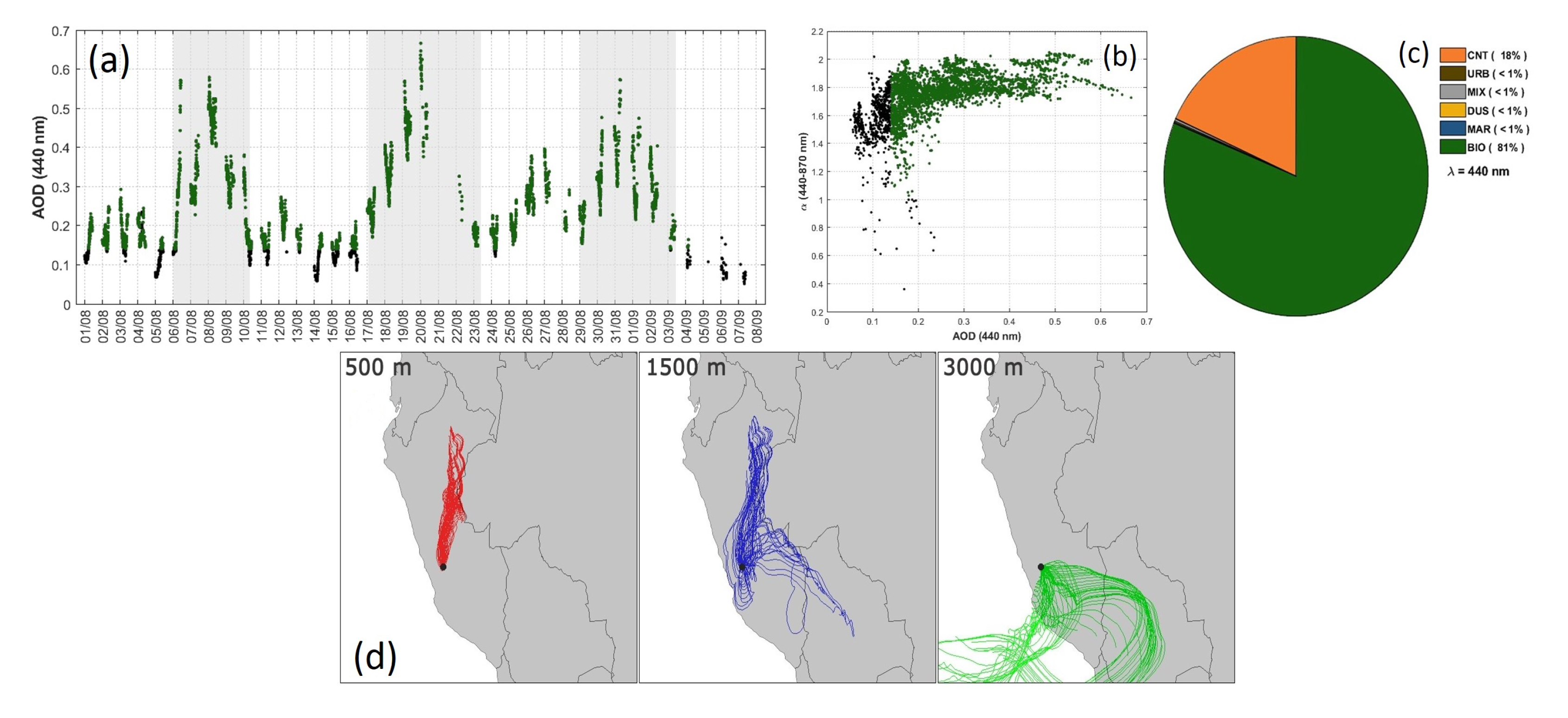
4.3. High Pollution Events

In 2019, between August and September, a large number of forest fires occurred in the Amazon region, mainly in Brazil and northern Bolivia. The large number of aerosols generated by these fires affected several regions of South America, including Peru. Several events with high aerosol loads were recorded during these months in the HYO, as shown in Figure 15a. The behavior of the AOD between 1 August and 8 September 2019 and, as can be seen, practically every day, the aerosols generated by the biomass burning (green dots) were recorded. A total of three events with high AOD values are highlighted, especially the ones recorded between August 17 and 23, where the maximum AOD value with a value of 0.67 recorded on August 20 at 12:30:56 UTC (07:30:56 LT) took place.
The aerosol classification determined from a scatterplot (Figure 15b) between AOD at 440 nm and the Angstrom Parameter within the range of 440–870 nm [15]. As can be seen in Figure 15c, the highest percentage of aerosols presence corresponds to the aerosols generated by the biomass burning (81%), followed by the Continental (CNT) aerosol type (18%). The remaining registered aerosols types during this period have a very little presence; in all cases, less than 1%. To determine the possible source regions where the aerosols registered during the aforementioned period were generated, the backtrajectories were calculated using the HYSPLIT model. The trajectories were calculated every three hours, 120 h backwards for each day between August 17 and 23, and for three altitude levels— 500, 1500, and 3000 m (Figure 15d). The NCEP-NCAR reanalysis was used as input meteorological data.
As can be seen in the figure, the trajectories of 500 and 1500 meter levels have their origin and pass through the Amazonian regions of Peru, and in the case of the 1500 m, level some trajectories pass over the northern region of Bolivia. In the case of the 3000 m trajectory, most of the trajectories also cross over the northern portion of Bolivia, where large forest fires were recorded during this period. In conclusion, it can be affirmed that the main source of biomass aerosols measured in the HYO between August 17 and 23 corresponds to the forest fires that took place in Peru itself with a certain level of contribution from the fires that had occurred in the northern region of Bolivia.

5. Discussions

5.1. Intense Rainfall Events

For the present contribution, we presented two intense rainfall events: the first one occurred on 17 January 2018 at 20 LT (RE1) with a maximum peak of 13.46 mm h 1 and the second one occurred on 28 December 2019 at 17 LT (RE2) with maximum peak of 12.1 mm h 1 . It is important to highlight that both events were succeeded (RE1) or preceded (RE2) by another intense rainfall event with only a few days in between. In addition, the amount of rainfall for both events was lower than the climatological (1965–2020) values of maximum daily accumulated rainfall, which were 42 mm day 1 for January and 47 mm day 1 for December. However, they were also similar to the climatological percentile 90% of daily accumulated rainfall, which were 14 mm day 1 for January and 13 mm day 1 for December [16]. The spatial distribution for both rainfall events were identified by the GPM system, a core of high rainfall rate of 7 mm h 1 above the HYO for both events (RE1 and RE2). For the RE1 event, four areas with high precipitation rates aligned from north-east to south-west were observed. In contrast, for the RE2 event, there were two areas of high precipitation rate aligned from north-west to south-east.
For both events, the patterns of reflectivity in function of height, measured by radars MIRA-35C and CLAIRE, demonstrated the presence of rainfall above the HYO. During the occurrence of an RE1 event, different types of rainfall (convective and stratiform) were observed. The convective rainfall with high values of reflectivity (40 dBZ) occurred at approximately between 1930 LT and 21 LT; meanwhile, the stratiform rainfall occurred approximately between 23 LT and 07 LT with values of reflectivity between 20 dBZ and 30 dBZ. In general, data from MIRA-35C was degraded by clouds and precipitation, as compared to the data from CLAIRE, due to its higher working frequency (35 GHz against 445 MHz) and, in consequence, it was necessary to make an attenuation correction. On the other hand, the PARSIVEL2 optical disdrometer, which measured the raindrop size distribution (RSD), allowed the estimation of rainfall rate (R), liquid water content (LWC), concentration total number (N t ), mass weighted mean diameter (D m ), intercept parameter (N w ) and reflectivity factor (Z) [9]. In addition, this set of parameters allows us to test different microphysical parameterizations from atmospheric numerical models and find the best performance against the in-situ observed data [36].
The mean synoptic conditions obtained from the GFS reanalysis data showed the important differences for both events (RE1 and RE2). For RE1, around the latitude of the HYO, strong easterly circulations at high levels (200 hPa), associated with the presence of the BH-NL system, were observed. On the contrary, for RE2, at high levels (200 hPa), it was found that there were observed strong westerly circulations and an absence of the BH-NL system around the location of the MB. These atmospheric configurations were identified in a recent study [10]. According to the results, RE1 corresponded to an easterly circulation (EC) event and RE2 to a westerly circulation (WC) event.

5.2. Intense Frosts Events

During frost events, the surface temperature of the ground or canopy falls below 0 C, and these events can be caused by in situ radiation cooling with clear skies and light winds (radiative events), as the atmosphere is open to the transmission of long-wave radiation (L * ), or advection of cold air to a region accompanied by strong winds (advective events) [37]. For the present study, we analyzed two intense frost events: the first one occurred on 21 June 2018 at 0603 LT (FE1) and the second on 5 April 2019 (FE2), at 0521 LT. For FE1 event, a continuous decrease in minimum temperatures during days before the occurrence of this frost event up to −3.0 C at a height of 2.0 m and 2.0 C at a height of 29 m. This behavior can be explained because the clear sky conditions above the HYO, estimated by the cloud product of MODIS sensor, during the days before and after the occurrence of this frost event, which corresponds to a radiative frost event [12].
In contrast, for the FE2 event, minimum temperature close to +0.23 C at a height of 2 m and +6 C at a height of 24 m. The minimum temperatures during the days before and after the occurrence of this frost event, corresponded to higher values close to 4 C at a height of 2 m, probably associated with the presence of high cloud fraction cover during the days preceding and following the occurrence of this frost event. The abrupt drop in minimum temperatures can be explained by the intrusion of cold surges from extra-tropical South America that move northward, accompanied by the progression of low-level winds and by a subsidence and dry conditions in the middle and low troposphere (1000–500 hPa) [14]. This cold and dry air arrived at the latitude of the MV (12 S) approximately at 00 UTC (19 LT) on 5 (4) April 2019, and intruded in central Andes a few hours later, which was observed by high intensities of wind speed in the early morning hours during FE2 event.
Moreover, during night hours and clear sky conditions, the surface loses more heat through radiation than the heat received from the air and subsoil [32]. Consequently, there is an abrupt drop in air temperature, which falls faster near the surface, causing temperature inversion. For FE1 event, during night hours, very stable conditions of the surface boundary layer were observed, with positive lapse rates of around +0.27 C m 1 and minimum mean hourly temperature (2 m high) close to −2.5 C at 07 LT. In contrast, for FE2 event, higher positive lapse rates with values close to +0.34 C m 1 and higher minimum mean hourly temperature (2 m high) of around +0.30 C at 06 LT were observed.
In addition, during some frost events, the water vapor profile may become inverted (positive lapse rates) near the surface under some conditions, such that vapor is transferred downwards as dew-fall. This process depletes moisture in the lowest layer of the atmosphere, while humidity decreases. For FE1 event, the positive lapse rate reached around +0.038 g kg 1 m 1 and the minimum water vapor mixing ratios at a height of 2 m, reached values close to 3.35 g kg 1 at 07 LT. In contrast, for the FE2 event, the positive lapse rates were lower, reaching +0.011 g kg 1 m 1 , but the minimum water vapor mixing ratios were higher at 5.03 g kg 1 at 06 LT. These differences can be explained by the seasonality of surface layer temperatures and moisture content in the HYO [13].
We highlighted that these minimum temperatures (−3.0 C for FE1 and +0.23 C for FE2) and minimum water mixing ratios (3.35 g kg 1 for FE1 and 5.03 g kg 1 for FE2) registered during FE1 and FE2 events were below the range of minimum mean monthly temperatures and water mixing ratios during June 2018 and April 2019, respectively (Figure 9). Moreover, due to the cooling of the surface by the emission of long-wave radiation, the lower air layers from the mountain slopes cool and slide down-slope due to the gravity pull as a result of katabatic wind of mountain-valley circulations inside the MV. During both of the extreme frost events (FE1 and FE2), the presence of a surface jet with maximum wind speeds of around 2.2 m s 1 at a height of 12 m, with maximum at 04 LT for FE1 and close to 2.3 m s 1 at a height of 29 m and with maximum at 02 LT for FE2 were observed.
In addition, both the mean hourly values and standard deviations of the surface energy balance components: net irradiance (Q * ), sensible heat flux (Q H ), latent heat flux (Q E ), and ground heat flux (Q G ), were lower than the mean monthly values and standard deviations of these components for both extreme frost events, during early morning hours before sunrise. This behavior was especially intense for Q * and Q E that showed strong negative values [12] as compared to the mean monthly values of these energy budget components for the same months of both frost events, which were estimated and analyzed for the HYO in a recent contribution [13].

5.3. High Pollution Events

By using a sun-photometer CIMEL CE-318T type, belonging to the AERONET [38], aerosol measurements have been performed since March 2015 on the HYO. Owing to these measurements, the definition of the period with the greatest presence of aerosols generated by the burning of biomass was possible. This period with high aerosol load was found to be between July and October, with September being the month with the maximum AOD values. The biomass-type aerosols registered in the HYO have their origin, mainly in the fires that had taken place in the Amazon region of Peru. However, under certain conditions, biomass aerosols originating in Brazil and northern Bolivia could reach the HYO.
These forest fires that had occurred in the Amazon release large amounts of gases and aerosols into the atmosphere, transported by air masses to regions distant from the fires that generated them, including several regions of South America such as the central Andes of Peru. In the present study, we analyzed three events with high values of AOD that occurred between 06 and 10 August, 17 and 22 August, and 29 August and 2 September 2019 on the HYO. The AOD values range from 0.55 to 0.65, which exceed the mean value of AOD that is equal to 0.10 ± 0.07 for the period of March 2015 to August 2017 [15]. Moreover, by using the HYSPLIT model [39,40,41], we estimated the possible source regions from where the aerosols registered on the HYO were generated. The trajectories showed that the main sources of biomass measured during the period of intense aerosol events in the HYO correspond to the forest fires that took place in Peru with certain contributions from the fires from the northern area of Bolivia.

6. Conclusions

The aim of this study was to present a set of the instruments to measure several physical, microphysical, and radiative properties of the atmosphere and clouds, which can be used to identify, understand, and subsequently, forecast and prevent the effects of extreme meteorological events, such as severe rainfall, hailstorms, frost, and high pollution events that can occur with some regularity in the regions of the central Andes of Peru, specifically in the MB. For this, the instruments were installed in the HYO, with the expectation to carry out observation field campaigns in different places of the MB, mainly in valleys and agricultural areas. According to the results and discussions presented above, we conclude the following:
Two intense rainfall events were analyzed; one occurred on 17 January 2018 at 20 LT and the other on 28 December 2019 at 17 LT. Both rainfall events were similar to the climatological (1965–2019) percentile 90% of daily accumulated rainfall. The patterns of reflectivity in function of height for both events were also shown, which were measured by radars MIRA-35C and CLAIRE, highlighting the presence of convective and stratiform rainfall types for both events. Moreover, the PARSIVEL2 optical measured the raindrop size distribution, which allows the estimations of several micro-physics parameters of convective and stratiform rainfall events. The GPM system was used to identify the spatial distribution around the Mantaro valley of both rainfall events. The first intense rainfall event was associated with strong easterly circulations at high levels (200 hPa) of the atmosphere, and the presence of the BH-NL system. In contrast, the second one was associated with the presence of strong westerly circulations and the absence of the BH-NL system around the location of the MRB.
In addition, we analyzed two intense frost events; one occurred on 21 June 2018, at 06 LT and the other on 5 April 2019, at 05 LT. The first one was mainly associated with the continuous clear sky conditions during the previous days of the frost event, above the HYO, corresponding to a radiative frost event. On the contrary, the second one was mainly associated with the intrusion of cold surges coming from extra-tropical South America. However, clear sky conditions was also observed one day before the occurrence of the frost event. In consequence, there was a combination of advective and radiative conditions for the second frost event. Moreover, the energy budget analysis of both the frost events revealed that the energy components were highly negative in comparison with the mean monthly values during the early morning hours. Finally, we presented a detailed analysis of three high pollution events that had occurred on the HYO between August and September in 2019. The HYSPLIT model, was used to identify the possible source regions where the aerosols registered on the HYO were generated, which correspond to the forest fires that took place in Peru with certain contributions from the fires in the northern area of Bolivia.
Taking these results into account, we concluded that the set of instruments of LAMAR can be used to identify and analyze the extreme meteorological events in other regions of the central Andes, mainly agricultural areas, by means of operational field campaigns. The adequate understanding of the physical processes, associated with the occurrence of extreme meteorological events, such as intense rainfall, frost, and high pollution events, can improve the ability of physical models to forecast the occurrence of these events and to plan strategies to mitigate the impact of those events on agricultural crops. Moreover, higher time and space scale observations of atmospheric variables performed by LAMAR instruments and better observations of key processes, including land–atmosphere interactions, can be used to improve global coverage of daily and sub-daily observations for temperature and precipitation extremes.

Author Contributions

For the present work, the contributions were distributed as follows: Conceptualization, J.L.F.-R., Y.S., D.S. and M.M.; Methodology, J.L.F.-R. and M.P.-L.; Software, R.E., J.L.F.-R. and J.V.-P; Validation, J.L.F.-R., J.V.-P and M.S.; Formal Analysis, J.L.F.-R., J.V.-P, M.S. and L.G.; Investigation, J.L.F.-R., M.P.-L., S.K. and L.G.; Resources, Y.S., L.S.-S. and R.E.; Data Curation, J.L.F.-R., J.V.-P, L.G. and M.S.; Writing—Original Draft, J.L.F.-R., M.P.-L., R.E., J.V.-P and M.S.; Writing—Review and Editing, J.L.F.-R., D.M.-C. and S.K.; Visualization, D.S. and M.M.; Supervision, Y.S., D.S. and M.M.; Project Administration, Y.S.; Funding Acquisition, Y.S. and L.S.-S. All authors have read and agreed to the published version of the manuscript.

Funding

Present study comes under the project “MAGNET-IGP: Strengthening the research line in physics and microphysics of the atmosphere (Agreement No 010-2017-FONDECYT)” This work was done using instruments of the Laboratory of Physics, Microphysics and Radiation (LAMAR) and computational resources, HPC-Linux -Cluster, from Laboratorio de Dinámica de Fluidos Geofísicos Computacionales at Instituto Geofísico del Perú (grants 101-2014-FONDECYT, SPIRALES2012 IRD-IGP, Manglares IGP-IDRC, PP068 program). Also, thanks to the Office of Antarctic Affairs of Ministry of External Affairs of Peru and WMO/GCOS programme for facilitating the implementation of BSRN station. We thank NASA Headquarters for their continuing support and long-term commitment to the AERONET project.

Institutional Review Board Statement

Not applicable.

Informed Consent Statement

Not applicable.

Data Availability Statement

The data presented in this study are available on request from the corresponding author.

Conflicts of Interest

The authors declare no conflict of interest.

Abbreviations

The following abbreviations are used in this manuscript:
AERONETAerosol Robotic Network
BSRNBaseline Surface Radiation Network
HYOHuancayo observatory
LAMARLaboratory of Atmospheric Physics, Microphysics and Radiation
MRBMantaro river basin
MVMantaro valley
GPMGlobal Precipitation Measurement
GFSGlobal Forecast System
GOESGeostationary Operational Environmental Satellite
MIRA-35CMETEK Meteorologische Messtechnik Radar
CLAIRECLear Air and Rainfall Estimations
BLTRBoundary Layer and Tropospheric Radar
ENSOEl Niño-Southern-Oscillation
WCRPWorld and Climate Research Programme
SALLJSouth America Low Level Jet

References

  1. Zhang, X.; Hegerl, G.; Seneviratne, S.; Steward, R.; Zwiers, F.; Alexander, L. WCRP Grand Challenge Science Underpinning the Prediction and Attribution of Extreme Events. 2014. Available online: www.clivar.org/sites/default/files/documents/wcrp/WCRPGrandChallengesExtremesrev.pdf (accessed on 19 March 2021).
  2. Alexander, L.; Zhang, X.; Hegerl, G.; Seneviratne, S. Implementation Plan for WCRP Grand Challenge On Understanding and Predicting Weather and Climate Extremes—The Extremes Grand Challenge. Available online: https://www.wcrp-climate.org/images/documents/grand_challenges/WCRP_Grand_Challenge_Extremes_Implementation_Plan_v20160708.pdf (accessed on 19 March 2021).
  3. Stocker, T.; Qin, D.; Plattner, G.K.; Tignor, M.; Allen, S.; Boschung, J.; Nauels, A.; Xia, Y.; Bex, V.; Midgley, P.E. IPCC, 2013: Climate Change 2013: The Physical Science Basis. Contribution of Working Group I to the Fifth Assessment Report of the Intergovernmental Panel on Climate Change, 1st ed.; Cambridge University Press: Cambridge, UK; New York, NY, USA, 2013. [Google Scholar]
  4. Sillmann, J.; Thorarinsdottir, T.; Keenlyside, N.; Schaller, N.; Alexander, L.V.; Hegerl, G.; Seneviratne, S.I.; Vautard, R.; Zhang, X.; Zwiers, F.W. Understanding, modeling and predicting weather and climate extremes: Challenges and opportunities. Weather Clim. Extrem. 2017, 18, 65–74. [Google Scholar] [CrossRef]
  5. Karoly, D. Science Underpinning the Prediction and Attribution of Extreme Events. 2016. Available online: https://www.wcrp-climate.org/documents/GC_Extremes.pdf (accessed on 19 March 2021).
  6. Garreaud, R. Multiscale analysis of the summertime precipitation over the central Andes. Mon. Weather Rev. 1999, 127, 901–921. [Google Scholar] [CrossRef]
  7. Junquas, C.; Takahashi, K.; Condom, T.; Espinoza, J.; Chavez, S.; Sicart, J.; Lebel, T. Understanding the influence of orography on the precipitation diurnal cycle and the associated atmospheric processes in the central Andes. Clim. Dyn. 2018, 50, 3995–4017. [Google Scholar] [CrossRef]
  8. Flores-Rojas, J.; Moya-Alvarez, A.; Kumar, S.; Martínez-Castro, D.; Villalobos-Puma, E.; Silva-Vidal, Y. Analysis of Possible Triggering Mechanisms of Severe Thunderstorms in the Tropical Central Andes of Peru, Mantaro Valley. Atmosphere 2019, 10, 301–331. [Google Scholar]
  9. Villalobos-Puma, E.; Martinez-Castro, D.; Flores Rojas, J.; Saavedra, M.; Silva Vidal, Y. Diurnal Cycle of Raindrops Size Distribution in a Valley of the Peruvian Central Andes. Atmosphere 2020, 11, 38. [Google Scholar] [CrossRef] [Green Version]
  10. Flores-Rojas, J.; Moya-Alvarez, A.S. Valdivia-Prado, J.; Piñas-Laura, M.; Kumar, S.; Karam, H.; Villalobos-Puma, E.; Martínez-Castro, D.; Silva, Y. On the dynamic mechanisms of intense rainfall events in the central Andes of Peru, Mantaro valley. Atmos. Res. 2020, 248. [Google Scholar] [CrossRef]
  11. Kumar, S.; Silva, Y.; Del-Castillo, C.; Flores-Rojas, J.; Moya-Alvarez, A.; Martinez-Castro, D. Precipitation structure during the life cycle of cloud systems over Peru using satellite based observations. Gisci. Remote Sens. 2020, 57, 1057–1082. [Google Scholar] [CrossRef]
  12. Saavedra, M.; Takahashi, K. Physical controls on frost events in the central Andes of Peru using in situ observations and energy flux models. Agric. For. Meteorol. 2017, 239, 58–70. [Google Scholar] [CrossRef]
  13. Flores-Rojas, J.; Cuxart, J.; Piñas-Laura, M.; Callañaupa, S.; Suárez-Salas, L.; Kumar, S.; Moya-Alvarez, A.; Silva, Y. Seasonal and Diurnal Cycles of Surface Boundary Layer and Energy Balance in the Central Andes of Perú, Mantaro Valley. Atmosphere 2019, 10, 779. [Google Scholar] [CrossRef] [Green Version]
  14. Espinoza, J.; Ronchail, J.; Lengaigne, M.; Quispe, N.; Silva, Y.; Bettolli, M.; Avalos, G.; Llacza, A. Revisiting wintertime cold air intrusions at the east of the Andes: Propagating features from subtropical Argentina to Peruvian Amazon and relationship with large-scale circulation patterns. Clim. Dyn. 2013, 41, 1983–2002. [Google Scholar] [CrossRef]
  15. Estevan, R.; Martínez-Castro, D.; Suarez-Sala, L.; Moya-Alvarez, A.; Silva, Y. First two and a half years of aerosol measurements with an AERONET sunphotometer at the Huancayo Observatory. Atmos. Environ. 2019, 3, 295–308. [Google Scholar] [CrossRef]
  16. Giráldez, L.; Silva, Y.; Zubieta, R.; Sulca, J. Change of the rainfall seasonality over Central Peruvian Andes: Onset, and, duration and its relationship with large-scale atmospheric circulation. Climate 2020, 8, 23. [Google Scholar] [CrossRef] [Green Version]
  17. Trasmonte, G.; Silva, Y.; Segura, B.; Latínez, K. Variabilidad de Las Temperaturas Máximas y Mínimas en el Valle del Mantaro. Memoria del Subproyecto “Pronóstico Estacional de Lluvias y Temperatura en La Cuenca del río Mantaro Para su Aplicación en la Agricultura", Primera ed.; Fondo Editorial CONAM-Instituto Geofísico del Perú; 2010; Available online: https://repositorio.igp.gob.pe/handle/20.500.12816/708 (accessed on 19 March 2021).
  18. Oscanoa, J.; Castillo, C.; Scipion, D. CLAIRE: An UHF wind profiler radar for turbulence and precipitation studies. Int. Congr. Electron. Electr. Eng. Comput. 2016. [Google Scholar] [CrossRef]
  19. Valdivia, J.; Scipion, D.; Milla, M.; Silva, Y. Multi-Instrument Rainfall-Rate Estimation in the Peruvian Central Andes. J. Atmos. Ocean. Technol. 2020, 37, 1811–1826. [Google Scholar] [CrossRef]
  20. Prakash, S.; Mitra, A.; Pai, D.; AghaKouchak, A. From TRMM to GPM: How well can heavy rainfall be detected from space? Adv. Water Resour. 2016, 88, 1–7. [Google Scholar] [CrossRef]
  21. Guo, H.; Chen, S.; Bao, A.; Behrangi, A.; Hong, Y.; Ndayisaba, F.; Hu, J.; Stepanian, P. Early assessment of integrated multi-satellite retrievals for global precipitation measurement over China. Atmos. Res. 2016, 176–177, 121–133. [Google Scholar] [CrossRef]
  22. Ma, Y.; Tang, G.; Long, D.; Yong, B.; Zhong, L.; Wan, W.; Hong, Y. Similarity and error intercomparison of the GPM and its predecessor-TRMM multisatellite precipitation analysis using the best available hourly gauge network over the Tibetan Plateau. Remote Sens. 2016, 8, 569. [Google Scholar] [CrossRef] [Green Version]
  23. Tang, G.; Zeng, Z.; Long, D.; Guo, X.; Yong, B.; Zhang, W.; Hong, Y. Statistical and hydrological comparisons between TRMM and GPM Level-3 products over a midlatitude basin: Is Day-1 IMERG a good successor for TMPA 3B42v7? J. Hydrometeor. 2016, 17, 121–137. [Google Scholar] [CrossRef]
  24. Chen, F.; Li, X. Evaluation of IMERG and TRMM 3B43 monthly precipitation products over mainland China. Remote Sens. 2016, 8, 472. [Google Scholar] [CrossRef] [Green Version]
  25. Sharifi, E.; Steinacker, R.; Saghafian, B. Assessment of GPM-IMERG and other precipitation products against gauge data under different topographic and climatic conditions in Iran: Preliminary results. Remote Sens. 2016, 8, 135. [Google Scholar] [CrossRef] [Green Version]
  26. Tan, J.; Petersen, W.; Tokay, A. A novel approach to identify sources of errors in IMERG for GPM ground validation. J. Hydrometeor. 2016, 17, 2477–2491. [Google Scholar] [CrossRef]
  27. Hobouchian, M.; Salio, P.; García Skabar, Y.; Vila, D.; Garreaud, R. Assessment of satellite precipitation estimates over the slopes of the subtropical Andes. Atmos. Res. 2017, 190, 43–54. [Google Scholar] [CrossRef]
  28. Manz, B.; Páez-Bimos, S.; Horna, N.; Buytaert, W.; Ochoa-Tocachi, B.; Lavado-Casimiro, W.; Willems, B. Comparative Ground Validation of IMERG and TMPA at Variable Spatiotemporal Scales in the Tropical Andes. J. Hydrometeorol. 2017, 18, 2469–2489. [Google Scholar] [CrossRef]
  29. Prueger, J.; Kustas, W. Aerodynamic Methods for Estimation Turbulent Fluxes, 1st ed.; USDA-ARS/UNL Faculty: Lincoln, NE, USA, 2005. [Google Scholar]
  30. Monin, A.; Obukhov, A. Basic laws of turbulent mixing in the ground layer of the atmosphere. Tr. Geofiz. Inst. Akab. Nauk 1954, 24, 163–187. [Google Scholar]
  31. Monteith, J. Dew. Q. J. R. Meteorol. Soc. 1957, 83, 322–341. [Google Scholar] [CrossRef]
  32. Oke, T. Boundary Layer Climates, 2nd ed.; Taylor and Francis Group: Oxfordshire, UK, 1987. [Google Scholar]
  33. Arya, S. Introduction to Micrometeorology, 2nd ed.; Academic Press: Cambridge, MA, USA, 1998. [Google Scholar]
  34. Foken, T.; Nappo, C. Micrometeorology, 1st ed.; Springer: Berlin/Heildelberg, Germany, 2008. [Google Scholar]
  35. Garay, O.; Ochoa, A. Primera Aproximación Para la Identificación de Los Diferentes Tipos de Suelo Agrícola en el Valle del Río Mantaro, 1st ed.; Instituto Geofísico del Perú: Lima, Peru, 2010. [Google Scholar]
  36. Martínez-Castro, D.; Kumar, S.; Flores-Rojas, J.L.; Moya-Álvarez, A.; Valdivia-Prado, J.; Villalobos-Puma, E.; Castillo-Velarde, C.; Silva-Vidal, Y. The Impact of Microphysics Parameterization in the Simulation of Two Convective Rainfall Events over the Central Andes of Peru Using WRF-ARW. Atmosphere 2019, 10, 442. [Google Scholar] [CrossRef] [Green Version]
  37. Garratt, J. The Atmospheric Boundary Layer, 2nd ed.; Cambridge University Press: Cambridge, UK, 1992. [Google Scholar]
  38. Holben, B.; Eck, T.; Slutsker, I.; Tanre, D.; Buis, J.; Setzer, A.; Vermote, E.; Reagan, J.; Kaufman, Y.; Nakajima, T.; et al. AERONET – a federated instrument network and data archive for aerosol characterization. Remote Sens. Environ. 1998, 66, 1–16. [Google Scholar] [CrossRef]
  39. Draxler, R. HYSPLIT4 User’s Guide; ERL ARL-230, NOAA Air Resources Laboratory: Silver Spring, MD, USA, 1999; Volume 60, pp. 1–254. [Google Scholar]
  40. Draxler, R. An overview of the HYSPLIT-4 modeling system of trajectories, dispersion, and deposition. Aust. Meteorol. Mag. 1988, 47, 295–308. [Google Scholar]
  41. Stein, A.; Draxler, R.; Rolph, G.; Stunder, B.; Cohen, M.; Ngan, F. NOAA’s HYSPLIT atmospheric transport and dispersion modeling system. Bull. Am. Meteorol. Soc. 2015, 96, 2059–2077. [Google Scholar] [CrossRef]
Figure 1. (a) The domain of the Mantaro river basin (MRB) and the Mantaro valley (MV). Geopolitical and altitude contours and the location of the HYO are indicated; (b) topography around the MV, with higher altitudes close to 5000 m asl.
Atmosphere 12 00408 g001
Figure 2. (a) Gradient tower located in the HYO with meteorlogical sensors installed at six height levels of 2, 6, 12, 18, 24 and 29 m; (b) tower located in the HYO with radiation sensors installed at 6 m high; (c) magnetron-based pulsed Ka-Band Doppler radar MIRA-35c; (d) boundary Layer and Troposphere Radar (BLTR). Both instruments are installed in the HYO since 2015; (e) Clear-Air and Rainfall Estimation (CLAIRE) radar; (f) optical disdrometer PARSIVEL. (g) Sun Sky Lunar Multispectral Photometer model CE318-T; (h) area of study and location of the instruments inside the HYO.
Atmosphere 12 00408 g002
Figure 3. (a) Time series of precipitation rate (mm h 1 ) obtained from an in situ pluviometer (red line) above the HYO during January 2018. (b) Monthly variation of hourly accumulated precipitation quantiles (boxplot) above the HYO. Green circles highlight the intensity and time of both the rainfall events on 17 and 18 January, 2018. The rainfall values are outliers that highly exceed the mean monthly precipitation of January, close to 1 mm h 1 . (c) Monthly and diurnal cycles of mean accumulated hourly precipitation above the HYO during the years 2017, 2018, and 2019. The dotted red lines indicate the time period when the greatest amount of rainfall occurs (15 LT to 21 LT). (d) Spatial distribution of precipitation rate (mm h 1 ) for the MV obtained from the GPM data for 17 January, 2018, at 21 LT. Longitudes, latitudes and contours of the MV and MB are indicated. The red circle indicates the location of the HYO.
Atmosphere 12 00408 g003
Figure 4. (a) Time series (UTC-5) of reflectivity (dBZ) obtained from the Magnetron-based cloud radar (MIRA-35C) (top figure) and CLAIRE (bottom figure) above the HYO for the event on 17 January 2018. (b) Time series of rain rate (mm h 1 ) (top figure) and reflectivity (dBZ) (bottom figure) obtained from PARSIVEL2 at a 2 m height, MIRA-35C at a 250 m height and CLAIRE at a 750 m height. (c) Time series of raindrop size distribution (mm) with a density of the particles obtained from the PARSIVEL2 (top figure), MIRA-35C (middle figure), and CLAIRE (bottom figure).
Atmosphere 12 00408 g004
Figure 5. Composites of wind streamlines (m s 1 ) and mean vertical velocities (Pa s 1 ) for the event on 17 January 2018 at 18 UTC (13 LT) for high levels: (a) 200 hPa, mid levels: (b) 500 hPa, (c) 700 hpa and low levels: (d) 950 hPa. Positive values indicate downdraft vertical winds and negative values indicate updraft vertical winds. All composites data were obtained from GFS-reanalysis data (resolution: 0.5 ). Longitudes, latitudes and contours of the MRB and Mantaro valley are indicated.
Atmosphere 12 00408 g005
Figure 6. (a) Time series of precipitation rate (mm h 1 ) obtained from an in situ pluviometer (red line) above the HYO during December 2019. (b) Monthly variation of hourly accumulated precipitation quantiles (boxplot) above the HYO. Green circles highlight the intensity and time of both rainfall events on 26 and 28 December 2019. The rainfall values are outliers that greatly exceed the mean monthly precipitation of January close to 0.5 mm h 1 . (c) Spatial distribution of precipitation rate (mm h 1 ) for the MV obtained from the GPM data for 28 December 2019, at 18 LT. Longitudes, latitudes and contours of the MV and MRB are indicated. The red circle indicate the location of the HYO. (d) Mean, maximum, minimum, percentile 10%, and percentile 90% of daily accumulated precipitation (mm day 1 ) between 1965 and 2019 on the HYO.
Atmosphere 12 00408 g006
Figure 7. Composites of wind streamlines (m s 1 ) and mean vertical velocities (Pa s 1 ) for the event on 19 December 2019 at 18 UTC (13 LT) for high levels: (a) 200 hPa, mid levels: (b) 500 hPa, (c) 700 hpa and low levels: (d) 950 hPa. Positive values indicate downdraft vertical winds and negative values indicate updraft vertical winds. All composites data was obtained from the GFS-reanalysis data (at a resolution: 0.5 ). Longitudes, latitudes, and contours of the MRB and MV are indicated.
Atmosphere 12 00408 g007
Figure 8. (a) Time series of air temperature ( C) at a height of 2 m and 29 m above the HYO between 19 June and 23 June, 2018. (b) Mean hourly vertical profiles of air temperature ( C) during night and early morning hours of 21 June 2018. (c) Mean hourly vertical profiles of water vapor mixing ratio (g kg 1 ) during night and early morning hours of 21 June, 2018. (d) Mean hourly vertical profiles of wind speed (m s 1 ) during night and early morning hours of 21 June 2018.
Atmosphere 12 00408 g008
Figure 9. (a) Monthly and diurnal cycles of mean hourly temperature ( C) at 2 m high above the HYO between July 2017 and July 2018. (b) Monthly variation of hourly minimum temperature quantiles (boxplot) at 2 m high above the HYO between July 2017 and July 2018. (c) Monthly and diurnal cycles of mean water vapor mixing ratio (g kg 1 ) at 2 m high above the HYO between July 2017 and July 2018. (d) Monthly variation of hourly water vapor mixing ratio quantiles (boxplot) at 2 m high above the HYO between July 2017 and July 2018. (e) Mean, minimum, maximum, percentile 10% and percentile 90% of minimum temperatures ( C) between 1965 and 2019 on the HYO.
Atmosphere 12 00408 g009
Figure 10. (a) Spatial distribution of cloud fraction obtained by MODIS sensor onboard of Terra satellite above the HYO for 19 January 2018 at 1455 UTC (955 LT). (b) Spatial distribution of cloud fraction obtained by MODIS sensor onboard of Terra satellite above the HYO for 20 January 2018 at 1540 UTC (1040 LT). One indicates completely overcast sky and zero indicates complete clear sky conditions. Longitudes, latitudes and geopolitical contours are indicated. Time series of cloud fraction obtained by MODIS sensor above the location of the HYO during (c) June 2018 and (d) April 2019.
Atmosphere 12 00408 g010
Figure 11. (a) Daily cycle of mean hourly values and standard deviations during 21 June 2018 of the energy balance components: net irradiance (Q * ), sensible heat flux (Q H ), latent heat flux (Q E ) and ground heat flux (Q G ). The mean hourly values of all components at 05 LT are shown. (b) Daily cycle of mean monthly values and standard deviations during June 2018 of the energy balance components. The mean monthly values of all components at 05 LT are shown.
Atmosphere 12 00408 g011
Figure 12. (a) Time series of air temperature ( C) at 2 m and 29 m high above the HYO between 3 April and 7 April 2019. (b) Mean hourly vertical profiles of air temperature ( C) during night and early morning hours of 5 April 2019. (c) Mean hourly vertical profiles of water mixing ratio (g kg 1 ) during night and early morning hours of 5 April 2019. (d) Mean hourly vertical profiles of wind speed (m s 1 ) during night and early morning hours of 5 April 2019.
Atmosphere 12 00408 g012
Figure 13. (a) Daily cycle of mean hourly values and standard deviations of the energy balance components on 5 April 2019: net irradiance (Q * ), sensible heat flux (Q H ), latent heat flux (Q E ), and ground heat flux (Q G ). The mean hourly values of all components at 05 LT are shown. (b) Daily cycle of mean monthly values and standard deviations during April 2019 of the energy balance components. The mean monthly values of all components at 05 LT are shown.
Atmosphere 12 00408 g013
Figure 14. Contours of pressure reduced to sea level (hPa) and contours of specific humidity (g kg 1 ) for South America (first column) on 4 April 2019 at 12 UTC (07 LT), (second column) on 5 April 2019 at 12 UTC (07 LT) and (third column) 6 April 2019 at 12 UTC (07 LT). Geopolitical contours are indicated.
Atmosphere 12 00408 g014
Figure 15. (a) AOD at 440 nm between 1 August and 8 September, 2019. Green dots represent the AOD related to biomass aerosols, and black dots represent the other aerosols types. (b) Scatterplot of AOD (440 nm) vs Angstrom parameter (440–870 nm) for aerosol classification. The green dots represent the classification of biomass aerosols and black dots other aerosols types. (c) Percentage of presence of each type of aerosol according to the classification performed. (d) Backtrajectories calculated with HYSPLIT for every days between 17 August and 23 August 2019 for three levels: 500, 1500 and 3000 m. Trajectories were calculated every 3 h and for 120 h backwards.
Atmosphere 12 00408 g015
Table 1. Characteristics of BLTR, CLAIRE and MIRA-35C radars.
CharacteristicsBLTRCLAIREMIRA-35C
Transmission PowerSolid state 30 kWSolid stated 5 kWMagnetron 2.5 kW
Operation frequency49.92 MHz445 MHz34.85 GHz
Beamwidth19.79 9.46 0.6
Range0.22–10 km0.52–6 km0.15–13 km
Range resolution75 m75 m31 m
Temporal resolution32.8 s23 s5.6 s
Table 2. Main characteristics of the meteorological instrumentation installed in the HYO.
Temperature ( C)Relative Humidity (%)Wind Speed (m s 1 )Wind Direction (degrees)Soil Heat Flux (W m 2 )Soil Temperature ( C)Soil Moisture (%)
SensorHMP60HMP6003002 Wind Sentry Set03002 Wind Sentry SetHFP01 soil heat flux plateDecagon 5TM VWCDecagon 5TM VWC
CompanyCampbell ScientificCampbell ScientificCampbell ScientificCampbell ScientificCampbell ScientificICT InternationalICT International
Range−40 to 600–1000–500–360±2000−40 to 500–100
Accuracy±0.63% for 0–90 5% for 90–100±0.5±1.0−15% to +5%±10.08 for 0–50 0.1 for 50–100
Table 3. Main characteristics of the radiation instrumentation installed in the HYO.
CMP10 PyranometerCHP1 PyrheliometerCGR4 Pirgeometer
CompanyKipp & ZonenKipp & ZonenKipp & Zonen
Spectral range (50% points)285 to 2800 nm200 to 4000 nm4500 a 42000 nm
Sensitivity7 to 14 V W 1 m 2 7 to 14 V W 1 m 2 5 a 15 V W 1 m 2
Response time<5 s<5 s<18 s
Directional response (up to 80 with 1000 W m 2 beam)<10 W m 2 --
Temperature dependence of sensitivity (−20 C to +50 C)<1%<0.5%-
Operational temperature range−40 C to +80 C−40 to +80 C−40 a +80 C
Maximum solar irradianciance4000 W m 2 4000 W m 2 -
Limites de irradiancia neta--−250 a + 250 W m 2
Publisher’s Note: MDPI stays neutral with regard to jurisdictional claims in published maps and institutional affiliations.

