Article

Extreme Rainfall Forecast with the WRF-ARW Model in the Central Andes of Peru

1
Subdirección de Ciencias de la Atmósfera e Hidrósfera, Instituto Geofísico del Perú, 15012 Lima, Peru
2
Systems Research Group Inc, College Park, MD 20740, USA
3
Servicio Nacional de Meteorología e Hidrología del Perú, 11076 Lima, Peru
4
Instituto de Meteorología de Cuba, 17500 La Habana, Cuba
*
Author to whom correspondence should be addressed.
Atmosphere 2018, 9(9), 362; https://doi.org/10.3390/atmos9090362
Submission received: 14 August 2018 / Revised: 13 September 2018 / Accepted: 14 September 2018 / Published: 18 September 2018
(This article belongs to the Section Meteorology)

Abstract

:
The ability of the WRF-ARW (Weather Research and Forecasting-Advanced Research WRF) model to forecast extreme rainfall in the Central Andes of Peru is evaluated in this study, using observations from stations located in the Mantaro basin and GOES (Geostationary Operational Environmental Satellite) images. The evaluation analyzes the synoptic conditions averaged over 40 extreme event cases, and considers model simulations organized in 4 nested domains. We first establish that atypical events in the region are those with more than 27 mm of rainfall per day when averaging over all the stations. More than 50% of the selected cases occurred during January, February, and April, with the most extreme occurring during February. The average synoptic conditions show negative geopotential anomalies and positive humidity anomalies in 700 and 500 hPa. At 200 hPa, the subtropical upper ridge or “Bolivian high” was present, with its northern divergent flank over the Mantaro basin. Simulation results show that the Weather Research and Forecasting (WRF) model underestimates rainfall totals in approximately 50–60% of cases, mainly in the south of the basin and in the extreme west along the mountain range. The analysis of two case studies shows that the underestimation by the model is probably due to three reasons: inability to generate convection in the upstream Amazon during early morning hours, apparently related to processes of larger scales; limitations on describing mesoscale processes that lead to vertical movements capable of producing extreme rainfall; and limitations on the microphysics scheme to generate heavy rainfall.

1. Introduction

Most of the rains in Peru are concentrated in the period between the months of September and April [1], defining a marked seasonality, with a dry season between May and August [2,3,4]. In general, rainfall plays a decisive role in agriculture in any region of the planet, and in the specific case of the Mantaro Basin of the central Andes of Peru, 71% of the arable land depends on the rainfall regime [5]. Having an accurate forecast of rainfall thus allows for a more adequate use of water resources, but also mitigates losses when extreme precipitation occurs, depending on the magnitude over a given period of time. The present investigation is directed to the forecast of extreme rainfall in the aforementioned region. In this area, the most intense rains occur during the rainy season, when deep-tropospheric moist air masses flow into the mountain ranges from the Amazon and converge during the afternoon, aided by valley and mountain circulations.
Extreme rainfall is that which, depending on the type of classification, exceeds a certain threshold for a specific region, either for a specific period of the year or independently from it. For example, in the case of Spain, where several authors have dealt with the issue of the intensity of extreme rainfall [6,7,8], the State Meteorological Agency considers “Moderate rain” to be between 2.1 and 15 mm/h; strong, between 15.1 and 30 mm/h; very strong, between 30.1 and 60 mm/h; and torrential when it precipitates more than 60 mm in one hour. Harnack in [9], for example, defined heavy rainfall episodes as those that had more than 51 mm of precipitation over an area of 10,000 km2 in a period of 1–2 days. Thus, the classification of extreme rainfall is subjective, but is generally based on regional climatologies.
The Peruvian Meteorological and Hydrological Service (SENAMHI) considers as “moderately rainy” those days (7:00 a.m.–7:00 a.m.) that exceed the 75th percentile but do not reach the 90th percentile, considers as “rainy” days where rainfall exceeds the 90th percentile but not the 95th percentile, and “very rainy” days those exceeding the 95th percentile, calculated from days with accumulated precipitation higher than the threshold of 1 mm [10]. For this work, a case was considered an “extreme” rainfall when at least one third of the stations recorded rainfall greater than the 90th percentile of its distribution.
Precipitation, like almost all meteorological variables at present, is predicted with the aid of global or regional numerical forecast models. In this paper, we evaluate the ability of the Weather Research and Forecasting model (WRF) [11] to forecast extreme short-term rainfall in the selected region, based on the classification adopted by SENAMHI.
The WRF model, developed as a collaboration of different institutions of the United States of America, is widely used in operational works and for research purposes, and is well-represented in international scientific literature. Thus, many works can be found about this model, particularly sensitivity studies about the influence of their physical schemes or domains resolution, special studies to assess its skill to reproduce particular extreme events in different regions, and other specific issues [12,13,14,15,16,17].
In this work, Section 2 describes the datasets and methodology, including the source of the rainfall data and the gridded data used for the synoptic analyzes, as well as the applied verification method. Section 3 shows the obtained results. In Section 3.1, a statistical description of the selected precipitation events is introduced, which includes the distribution of the number of cases and the maximum values recorded by months, as well as the distribution of the number of events for different precipitation intervals and a box diagram. In Section 3.2, the synoptic patterns associated to the rain events taken for the study are shown, including the maps of geopotential, wind, and relative humidity at different levels, as well as the anomalies of their average fields during the cases of extreme rainfall relative to the average fields for the rainy season in Peru. Although it is not the objective of the present investigation, it is useful to dedicate a space to the synoptic patterns associated with extreme rainfall events, since it is the general circulation that gives rise to the basic conditions of the different weather states, and they even condition the local circulation. This has been discussed for South America in [18,19,20]. Statistical results about the model’s ability to detect extreme rainfall, including two case studies, are presented in Section 3.3.

2. Data and Methods

2.1. Analyzed Heavy Precipitation Events

Precipitation data were taken from 30 meteorological surface stations of the official database of the meteorological observations network of SENAMHI, whose geographical distribution is shown in Figure 1. In order to select the cases, the applied criterion was that the 24 h rainfall recorded in a station exceeded the 90th percentile of its climatology, and this holds at least in one third of the stations. This condition was introduced to ensure that precipitation has not been a very local process. The selected cases are shown in Table 1.
The average synoptic conditions associated to the extreme rainfall events at 1200 UTC (Universal Time Coordinated) over the period 1981–2017 were described using gridded reanalysis data from the National Center for Environmental Prediction and Atmospheric Research [21].

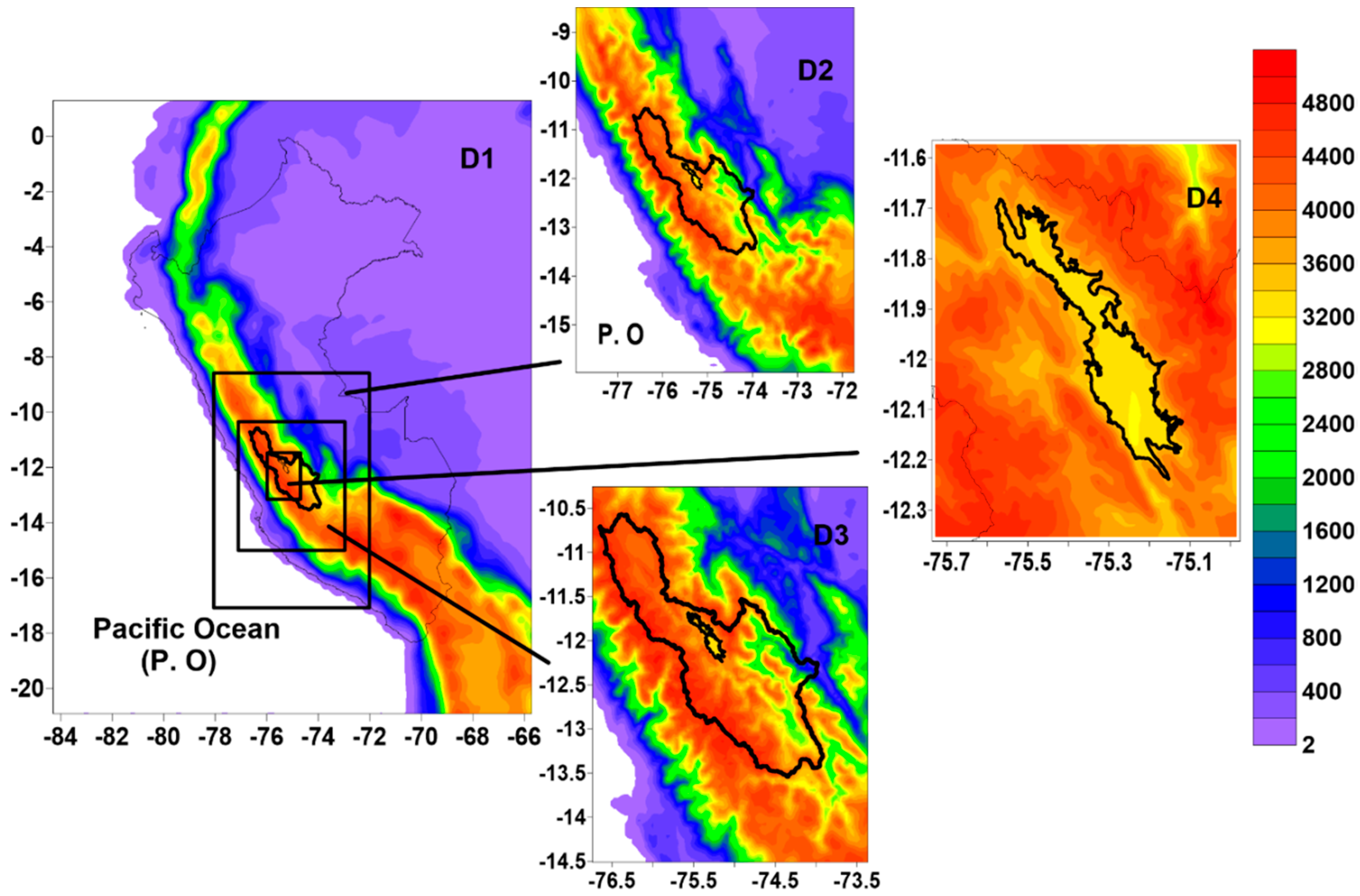
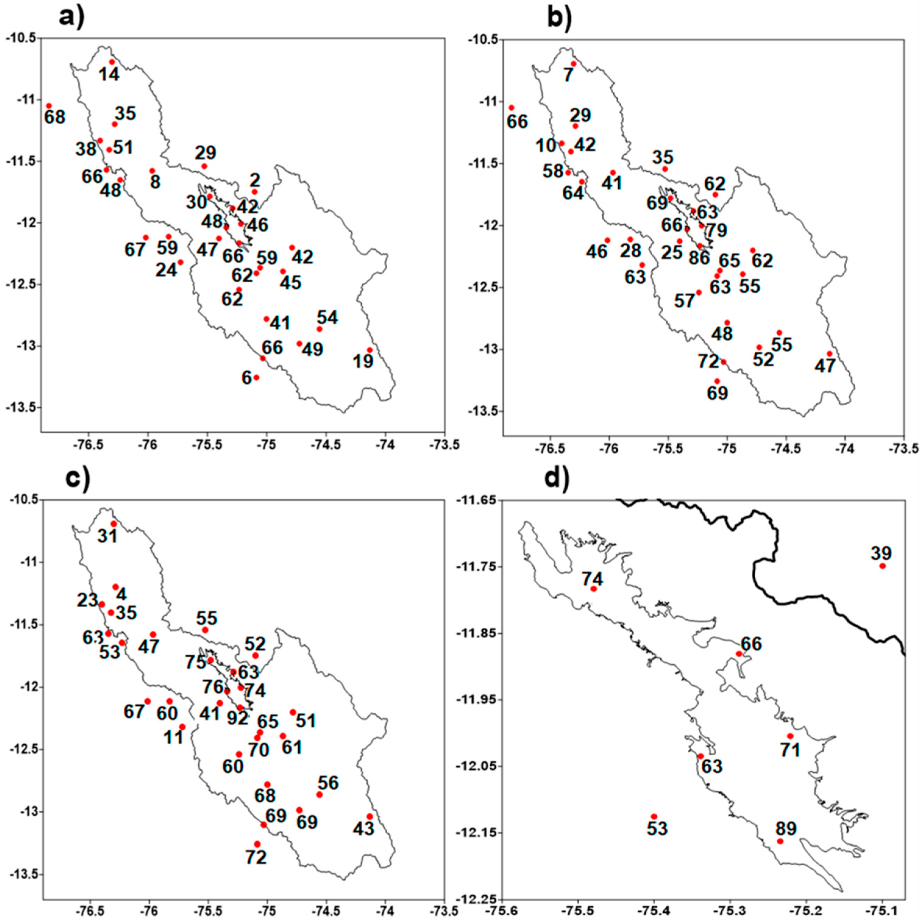
2.2. Meteorological Forcing Data, Domains, and Model Configuration

The experiments were conducted with the model WRF_ARW V.3.7 for 40 selected cases of extreme rainfall. The initial and boundary conditions were taken from the Global Operational Final Analyses (FNL) of the National Center of Environmental Prediction (NCEP) (available online at https://rda.ucar.edu/datasets/ds083.2/), which has a temporal resolution of 6 h and a horizontal resolution of 1° × 1°.
The model topography was constructed with the topographic dataset of the digital elevation model of the Shuttle Radar Topography Mission (available online at SRTM; https://dds.cr.usgs.gov/srtm/version2_1/), which has a resolution of 90 m [22,23].
The simulations were produced for four domains (Figure 2), whose characteristics are specified in Table 2. It should be noted that D4 only covers 7 of the 30 stations considered. The nesting was built by applying the unidirectional technique, where the external domain provides boundary data to the internal domain, but there is no feedback. The model was initialized at 00 UTC for all cases (approximately between 14 and 16 h before the expected onset of convection) with a forecast horizon of 36 h.
The parameterization schemes were selected based upon previous works [17] and considering results under similar conditions of complex orography in tropical regions [24,25,26,27]. Accordingly, the Morrison scheme was used for microphysics [28]; The YSU (Yonsei University Scheme) scheme, described in [29], was used for the boundary layer; and the MM5 Similarity Scheme [30,31,32,33,34] for the surface layer. The RRTMG (Rapid Radiative Transfer Model) [35], was used as a radiation model, and the Grell-Freitas scheme for convection [36]. The soil model was the so-called Unified Noah Land Surface Model [37]. In this sense, Weisman et al. in [38], considered that organized convective structures could be explicitly solved with grids spacing finer than 4 km. However, Molinari and Dudek in [39] argued that the use of explicit methods only transfers the problem to microphysical schemes and turbulence. A short experiment conducted in [17] for the present study region found that choosing whether or not to deactivate the cumulus parameterization scheme was irrelevant. Belair and Mailhot in [40] found that the resolution of 2 km, with an explicit scheme for cumulus, significantly overestimated the precipitation for a line of convective instability. Something similar was obtained in [41]. Since the studies cited above lean towards deactivation at high resolutions, the cumulus parameterization scheme was deactivated for the 3 and 0.75 km domains.

2.3. Model Verification

Verification of the results was applied to 24 h precipitation accumulations, using numerical descriptive statistical metrics: bias (B), root mean squared error (RMSE), and mean absolute error (MAE). In this case, model output was compared with observed precipitation. For this, the 40 modeled output data were interpolated to the station grid points using the Cressman method, that is, a simple and computationally fast method which is generally more accurate than other similar methods. However, this method can produce unrealistic edges in the grids near the edges of the spatial domain [42]. To avoid this problem, the domains in the present investigation were built in such a way that the stations considered were far from their borders. This verification method will henceforth be called point verification.
An additional experiment (independent of the 40 cases) was conducted to determine the relationship between the model bias and the observed precipitation. The objective was to define the point of change of the model bias’ sign and to know from which threshold, on average, the model would begin to underestimate accumulations. For the experiment, 9 sets of data belonging to the rainy period were considered, each with a forecast horizon of 10 days. The periods were selected so that they contained rainy and less rainy days in order to try and find the threshold value for which the model began to underestimate rainfall. These were selected between the months of December and February of the years 2007, 2009, 2010, 2011, and 2012. This period includes rainy years (2010 and 2011), and less rainy years (2007, 2009, and 2012). Also, as the data were taken from a 10-day forecast, it was considered that the bias remained relatively stable over time during the whole period [17]. The selected ten-day periods are listed below:
  • First ten of January of 2007.
  • Second ten of January of 2007.
  • Second ten of February 2007.
  • Third ten of December 2007.
  • Second ten of February 2009.
  • First ten of February 2010.
  • Third ten of February 2010.
  • Third ten of January 2011.
  • First ten of February 2012.
In addition, considering the results of the general statistical analysis of the research, it was decided that two experiments would be carried out with case studies, with the objective of investigating the causes of the processes that gave rise to extreme events with a greater level of detail. In that sense, the events of 11 February 2011 and 22 March 2009 were selected, in which the model significantly underestimated the recorded rainfall. To enhance the inter-comparison exercise, infrared GOES satellite images were evaluated in addition to the use of the station precipitation observations.

3. Results and Discussion

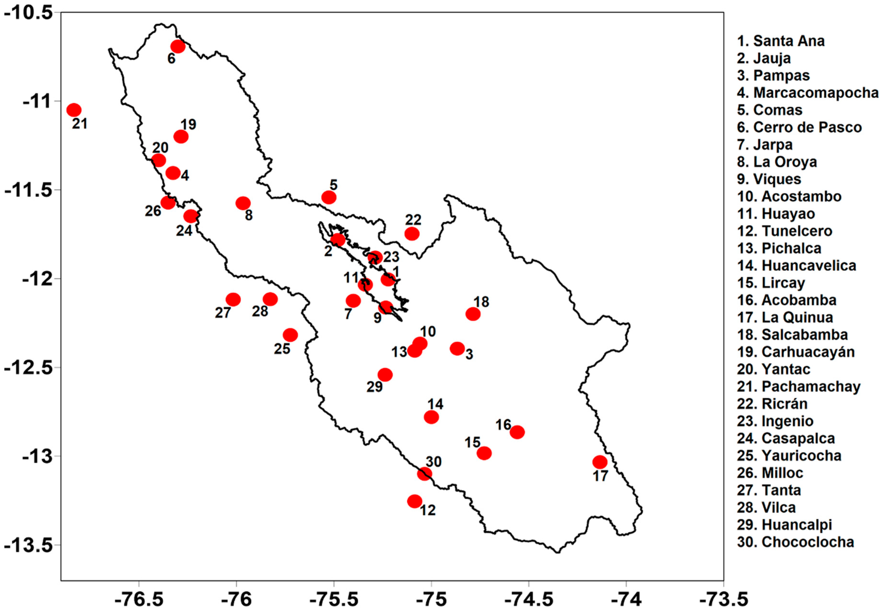
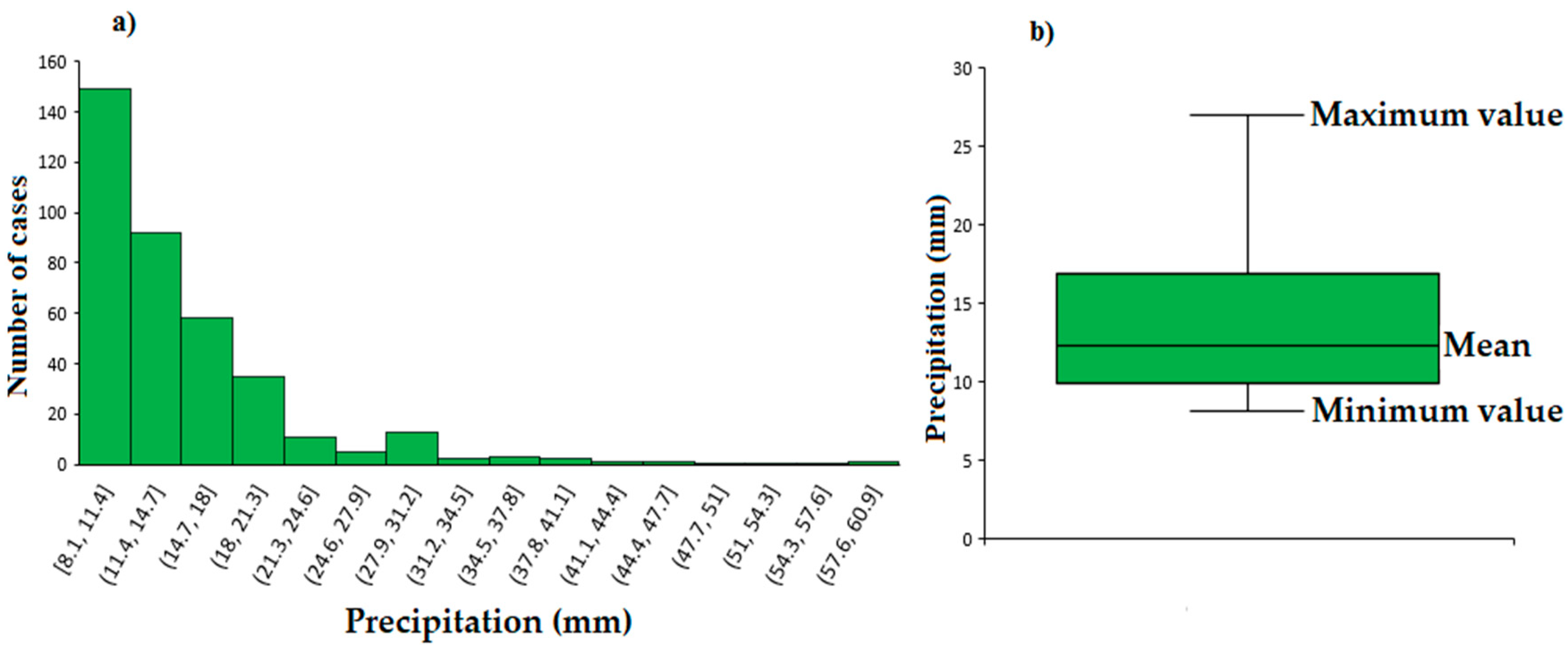
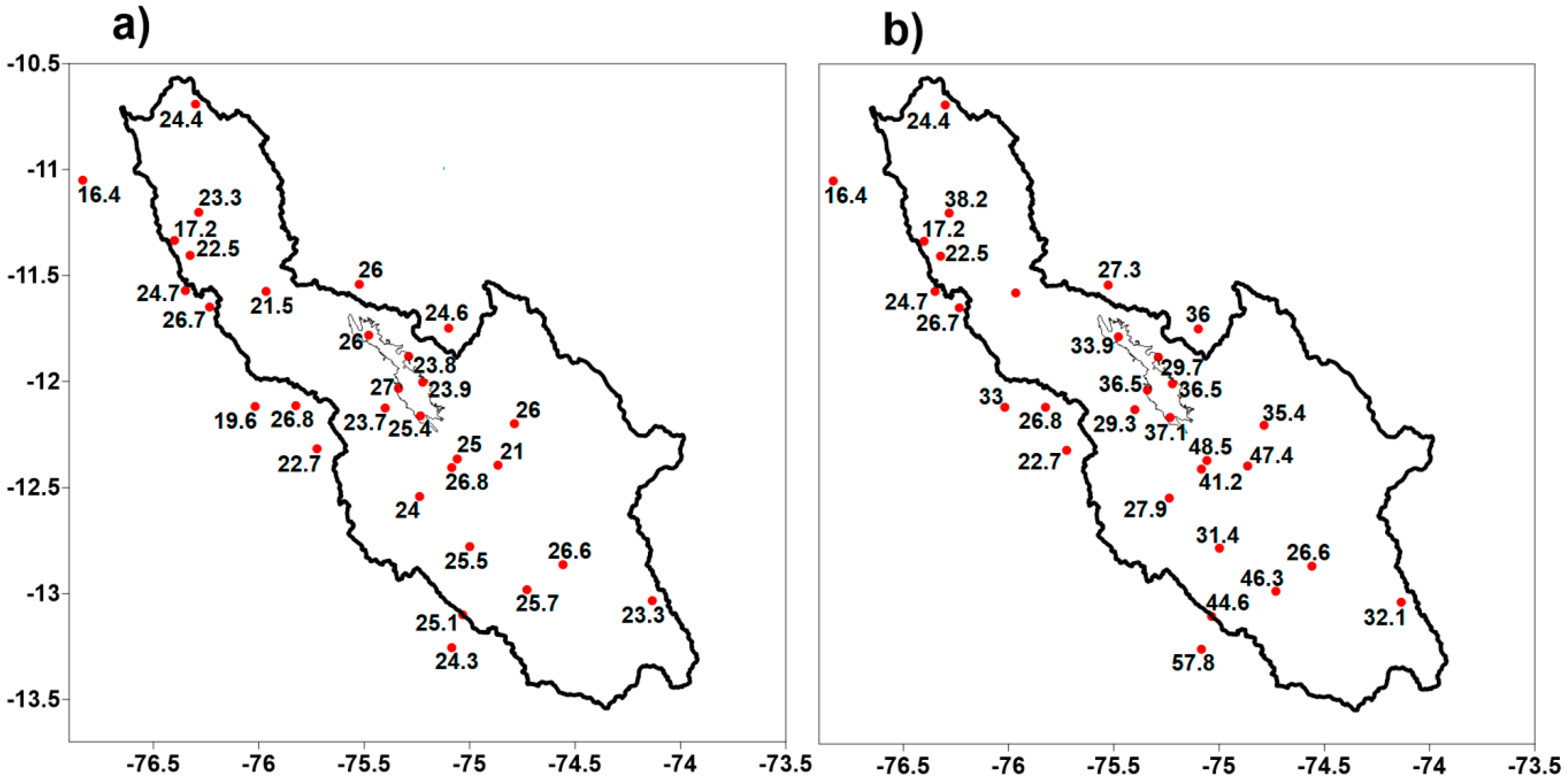
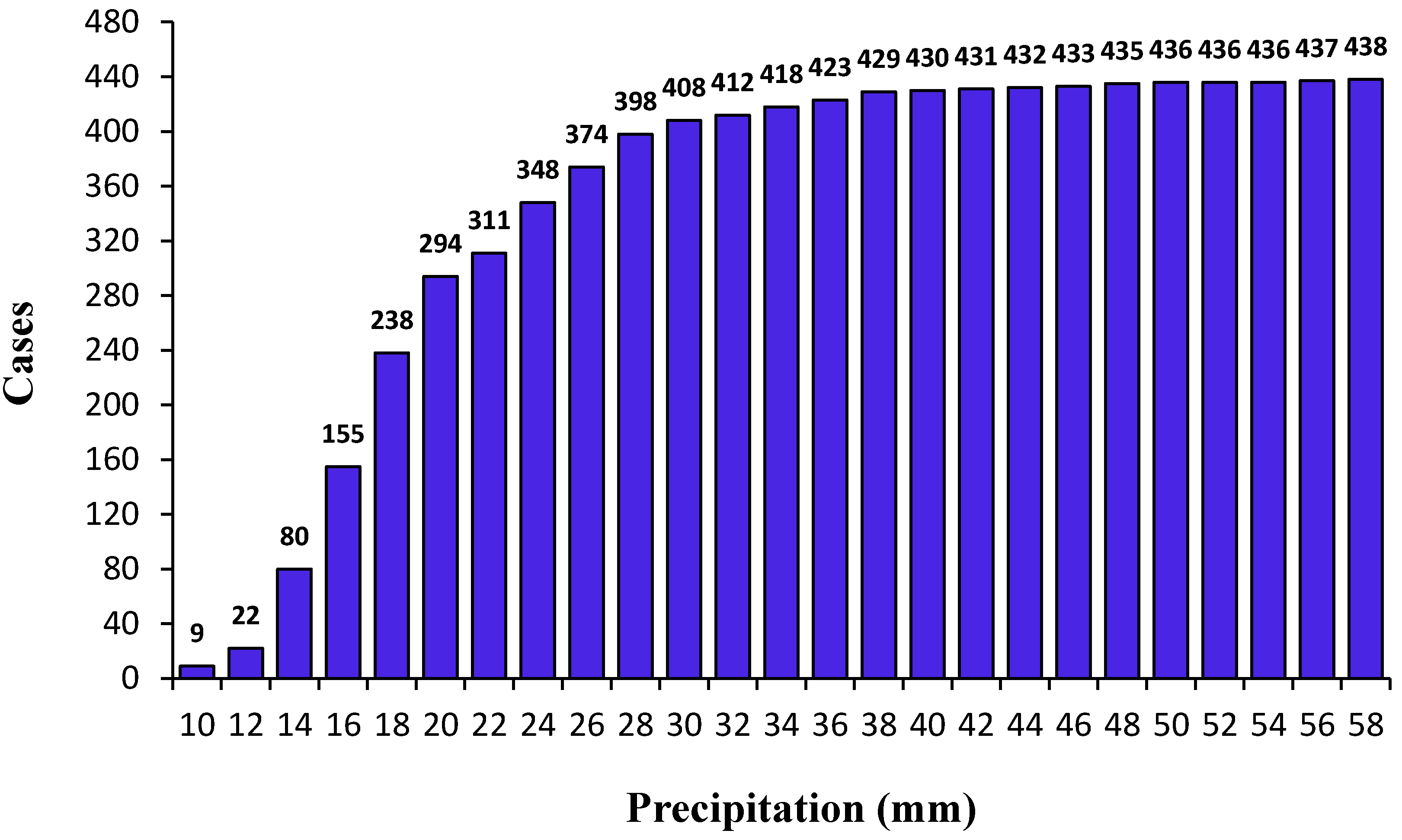
3.1. Extreme Rainfall in the Mantaro Basin

Figure 3 shows the monthly distribution of the 40 cases selected for the study. Eight cases occurred in the months of January, February, and April, 6 in December and March, and 4 in November. The January and February cases coincided with the rainiest period of the year. Figure 4 further shows that the most extreme events in terms of single-station 24 h accumulated precipitation occurred in these two months.
Figure 5 shows the box diagram of the extreme rainfall series considered in the investigation, in which it can be observed that the distribution is asymmetric and that precipitation values above 27 mm are approximately atypical. A daily rainfall value was considered as an outlier if it was two standard deviations greater than the mean value.
The spatial distribution of the mean and maximum accumulations registered is shown in Figure 6. Here, the outliers were removed to calculate the means, as in Figure 5b. In this case, it is evident that the maximum records are concentrated towards the southern half of the basin. The maximum value (57.8 mm) was recorded in Tunelcero, precisely where the southernmost station is located, and in the region of the western mountain range.

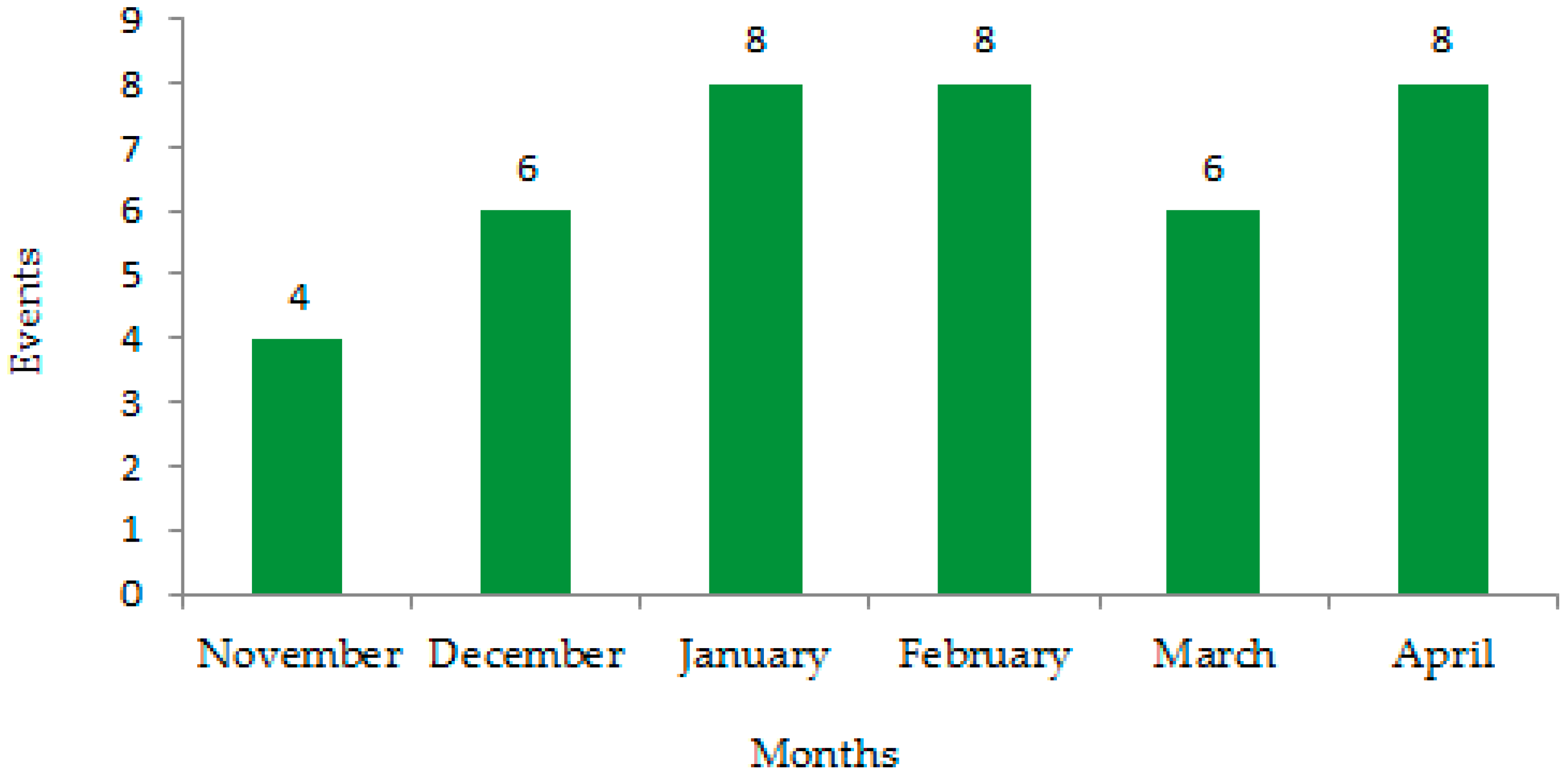
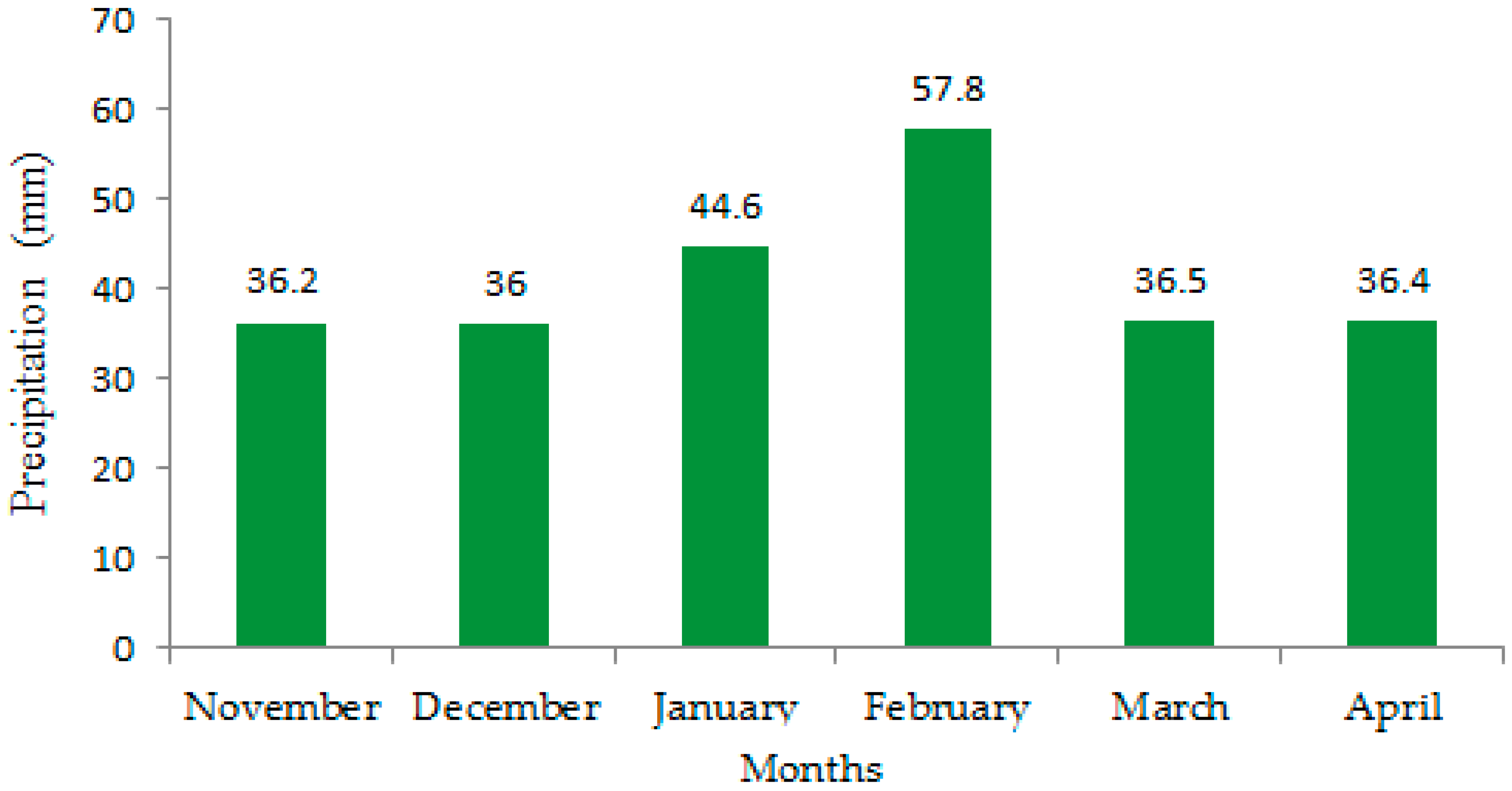
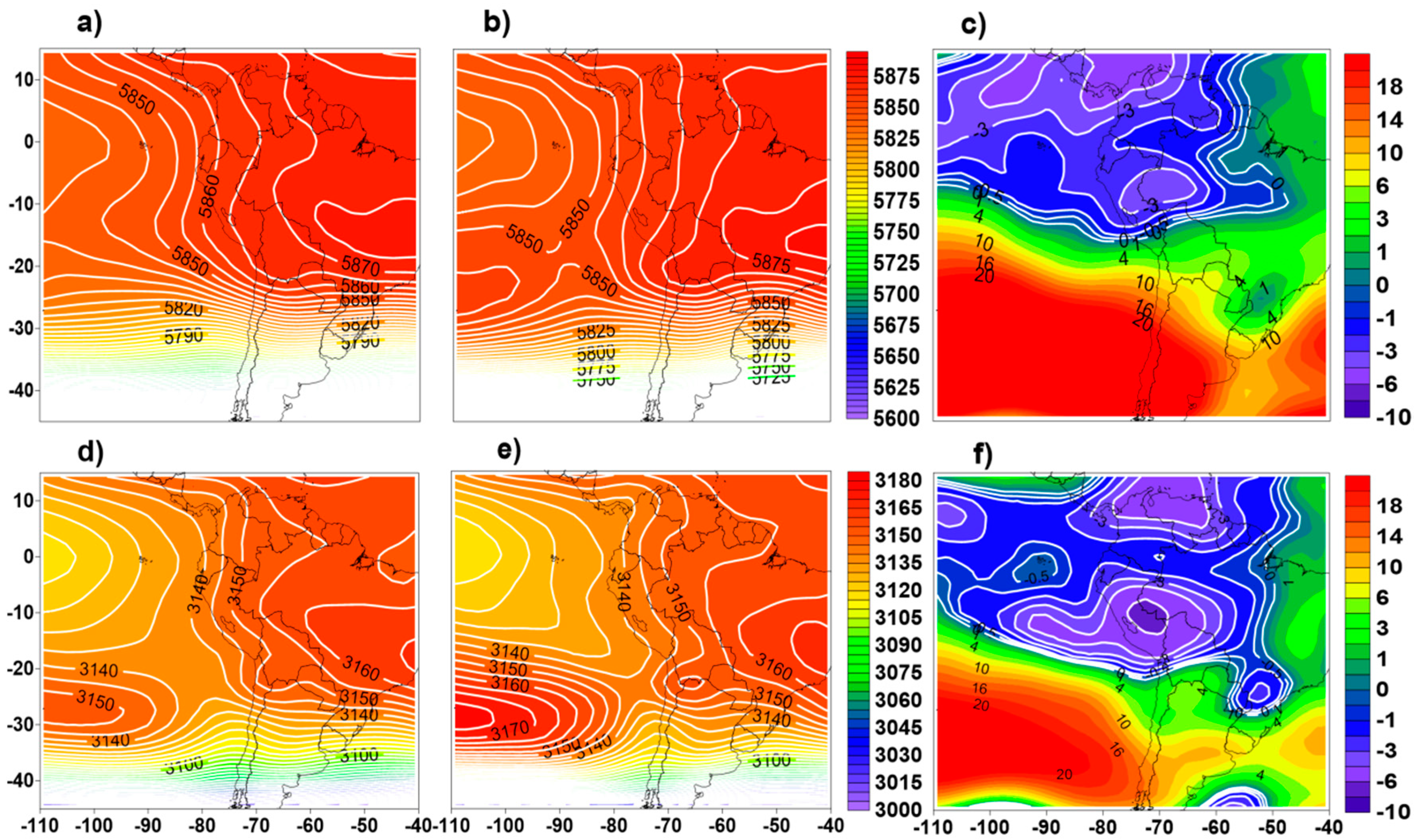
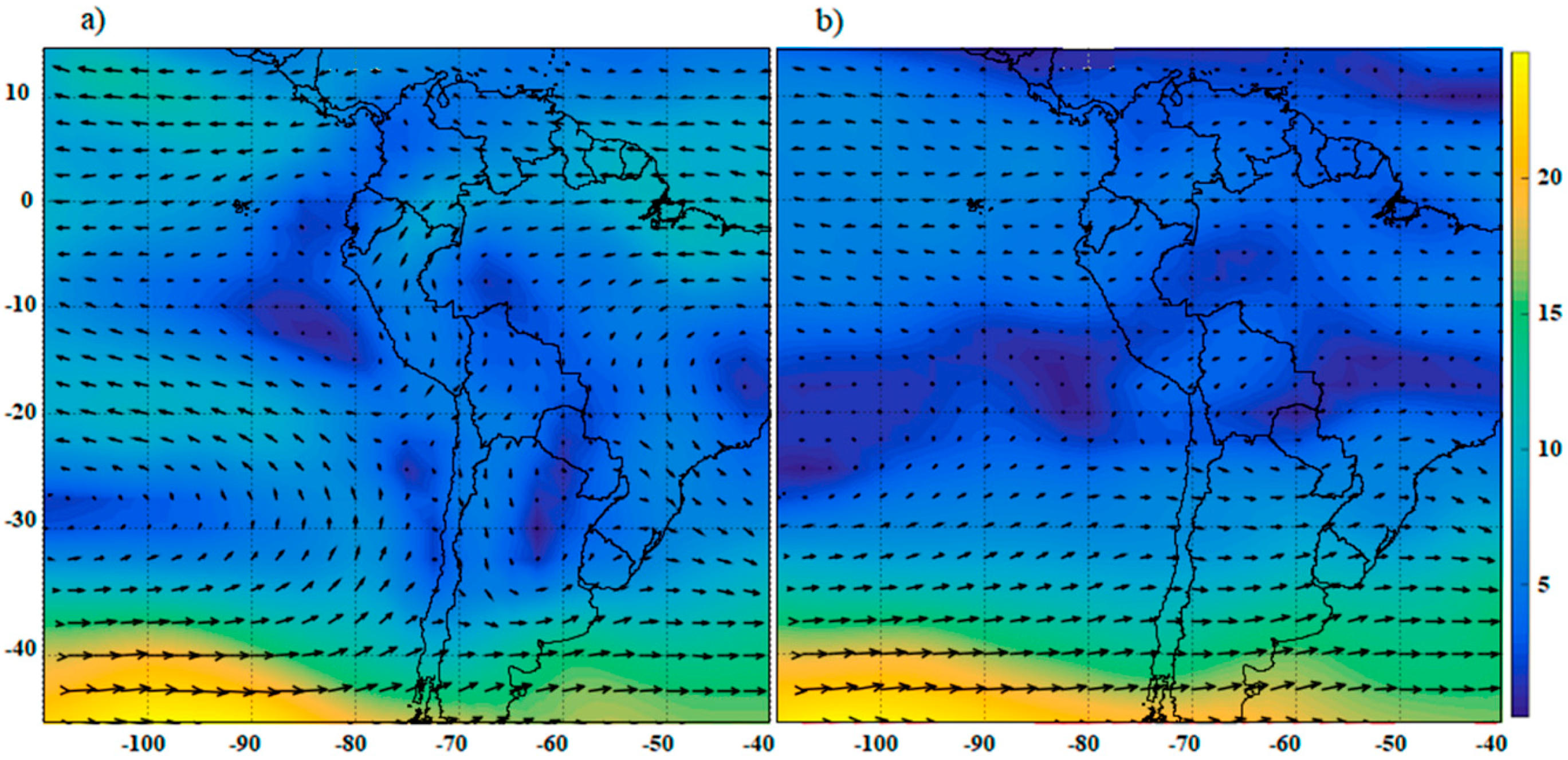
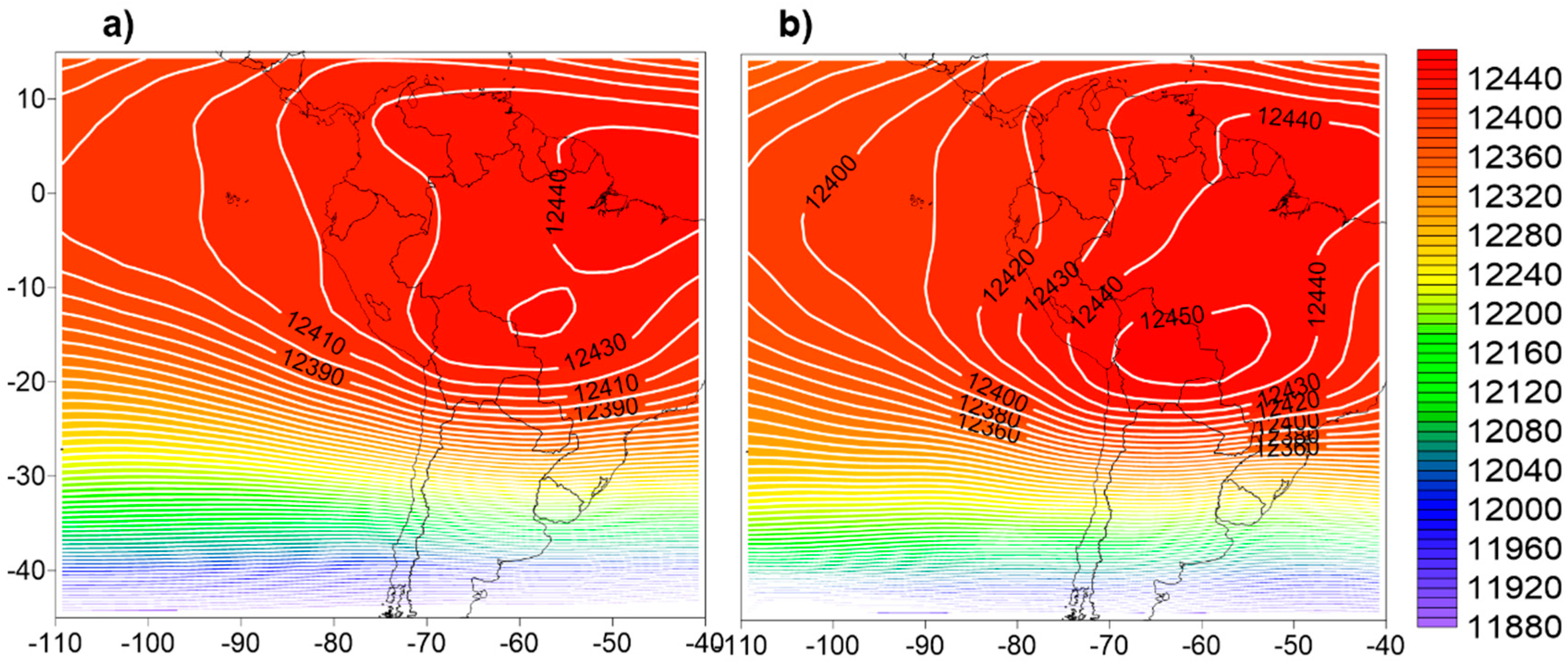
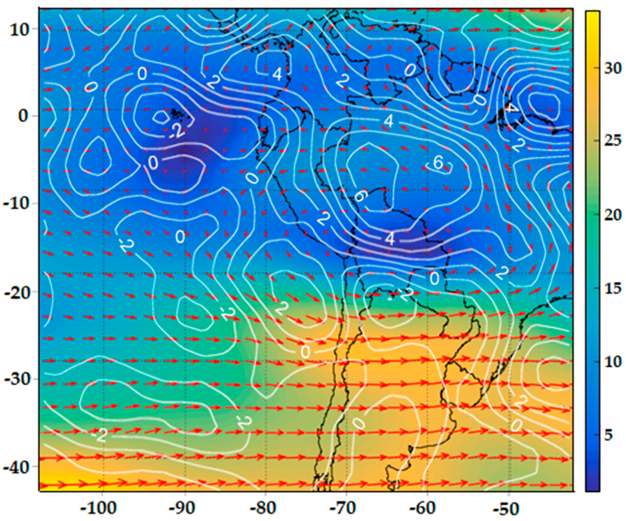
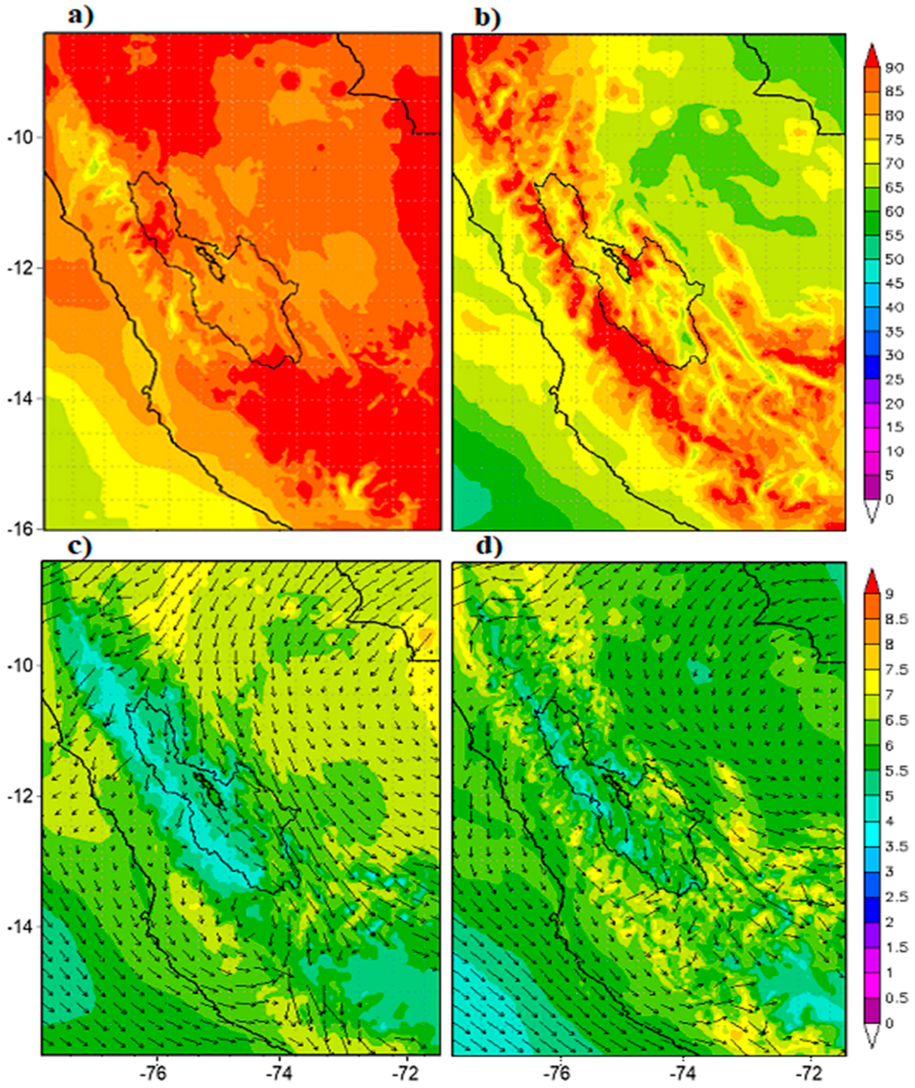
3.2. Synoptic Climatology Associated with the 40 Extreme Rainfall Events Cases Selected

Synoptic climatology charts were constructed with NCEP-NCAR (National Centers for Environmental Prediction-National Center for Atmospheric Research) reanalysis data by averaging over the 40 extreme rainfall event cases selected. Corresponding anomaly charts were then calculated by removing rainy season climatologies calculated over the 1981–2017 period. The findings are discussed in the following.
Figure 7 shows 500 and 700 hPa geopotential height composites, which are consistent with the associated flow charts shown in Figure 8. An analysis of both levels suggests that, during extreme rainfall events, the mid-tropospheric ridge lies displaced to the south and east, forming a cell in eastern Brazil and another over southern Altiplano. This mid-tropospheric geopotential and associated flow pattern stimulates the inflow of Amazonian air masses, generally moist, into the Andes of south and central Peru. To confirm this, the corresponding average (a) and anomalous (b) relative humidity fields of the 700–500 hPa layer are presented in Figure 9. These reflect high values over Peru and the western half of Brazil. Relative humidity anomalies lie in the 8–12% range in the southern half of Peru and in upstream regions of the Amazon. These results suggest that the combination of large-scale geopotential/flow anomalies and the presence of moist air masses over and upstream of the central Andes of Peru are linked to an increase in precipitation in the Mantaro Basin. Here, moisture transport from the Amazon can play an important role [43]. Figure 7b,d,e and Figure 8a,b also shows a mid-tropospheric trough that extends from the tropical eastern Pacific further into the west coasts of Peru and northern Chile. The corresponding anomaly charts show anomalous low heights over central Peru, with a large area of negative height anomalies exceeding 6 and 3 m at 700 and 500 hPa respectively.
Furthermore, an analysis of 200 hPa geopotential height and the associated flow are summarized in Figure 10 and Figure 11. They show a stronger subtropical upper ridge or “Bolivian high”, as well as a westward displacement of its center. This positions its northern divergent flank over Peru, which stimulates ascent in the mid and upper troposphere.
Thus, in general, the average synoptic configuration of the 40 extreme rainfall event cases indicates favorable conditions for enhanced precipitation in relation to average rainy-season conditions. The average captured the signals of (i) an enhanced moist flow from the Amazon basin, (ii) reinforced convergence and diurnal circulations over the mountain range, and (iii) enhanced ascent favored by the divergent northern flank of the subtropical upper ridge or Bolivian high.

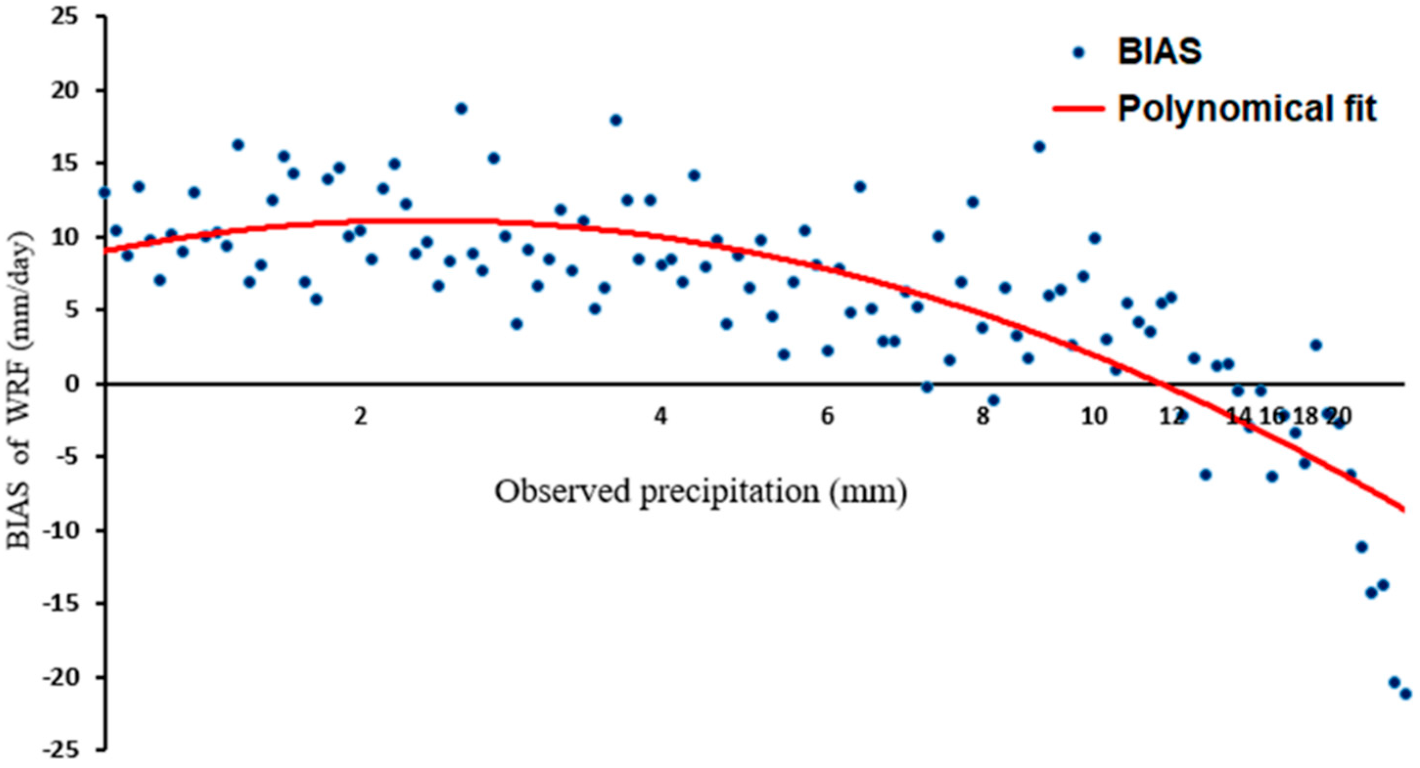
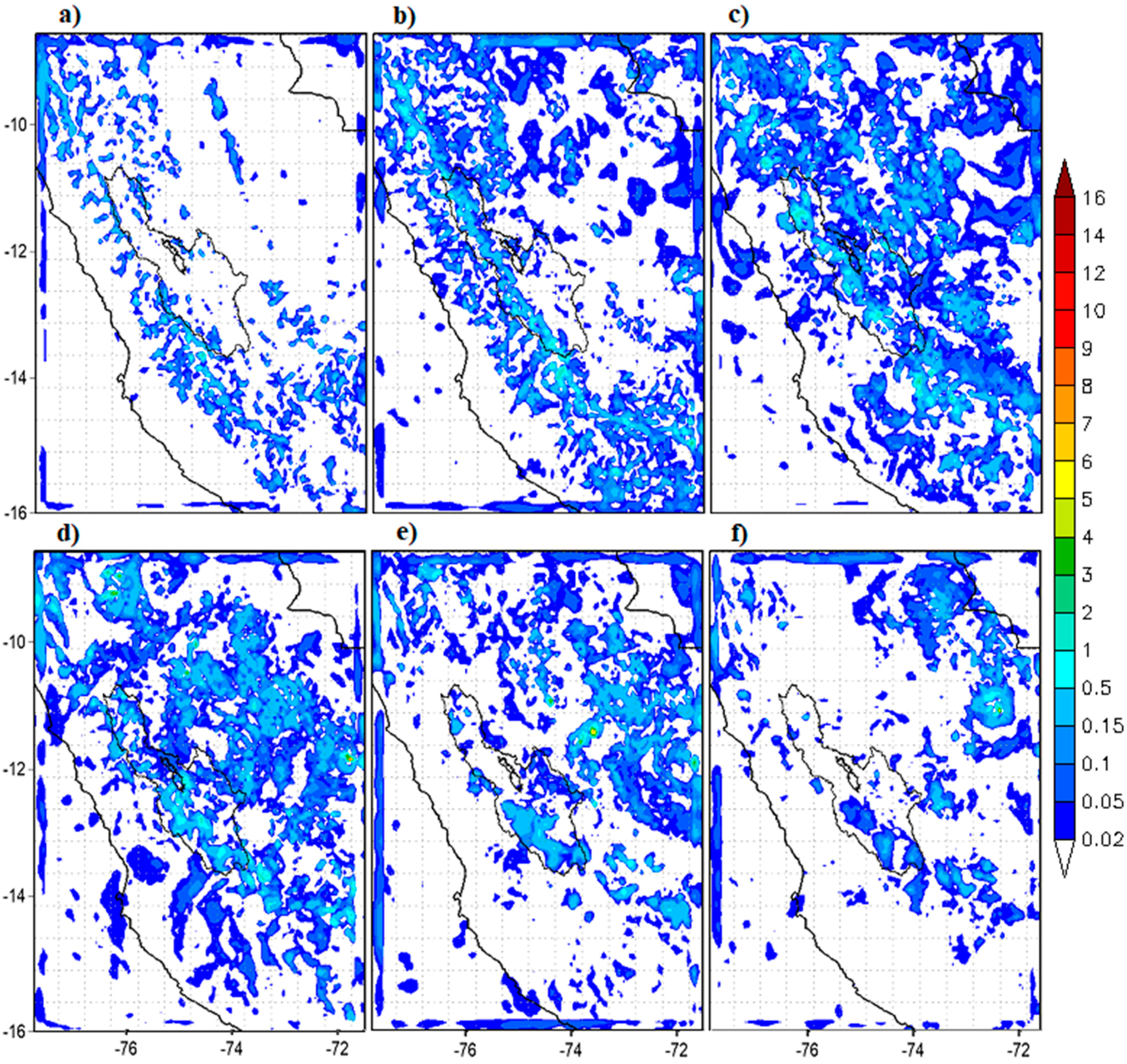
3.3. WRF Ability to Detect Extreme Rainfall
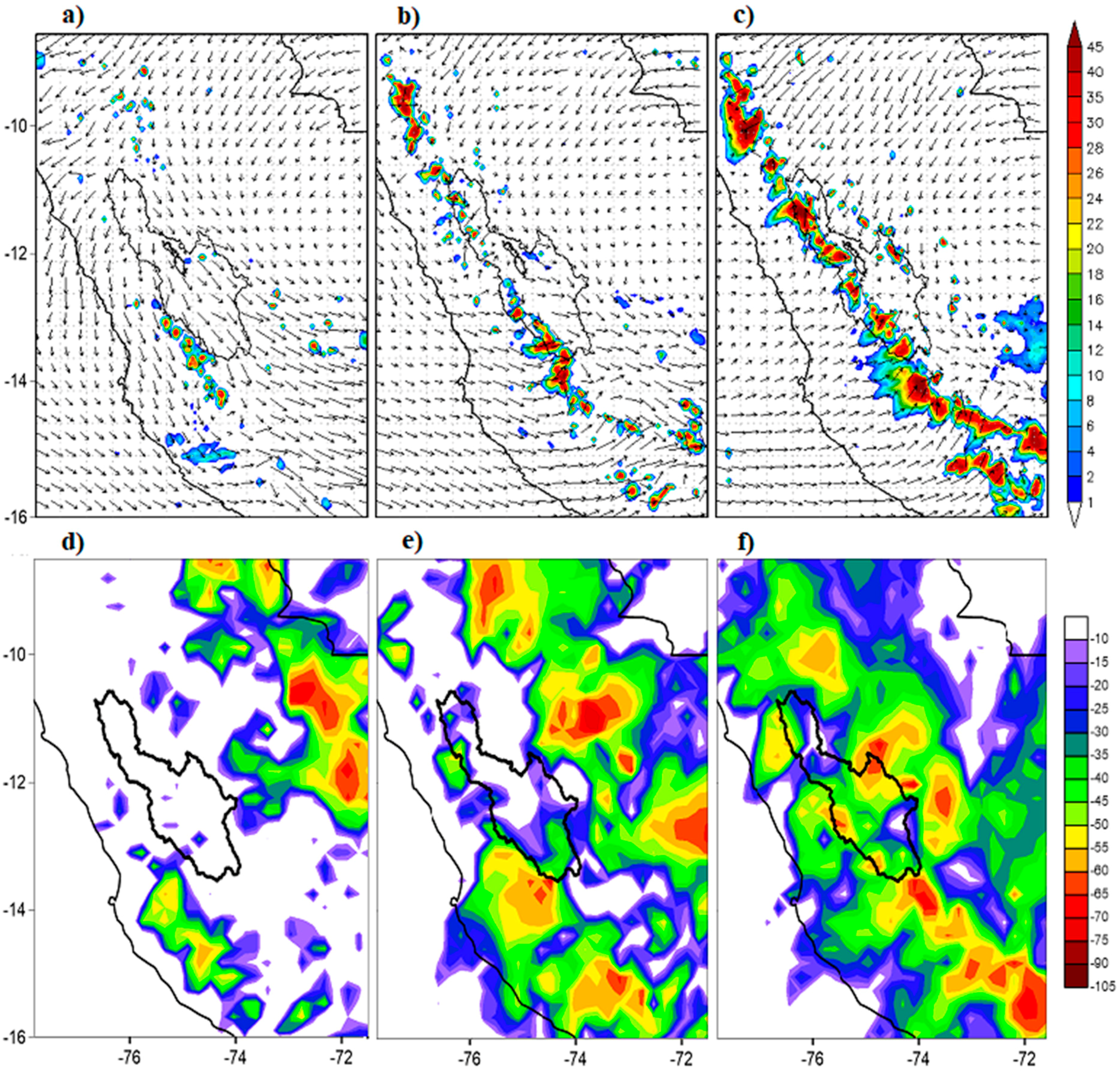
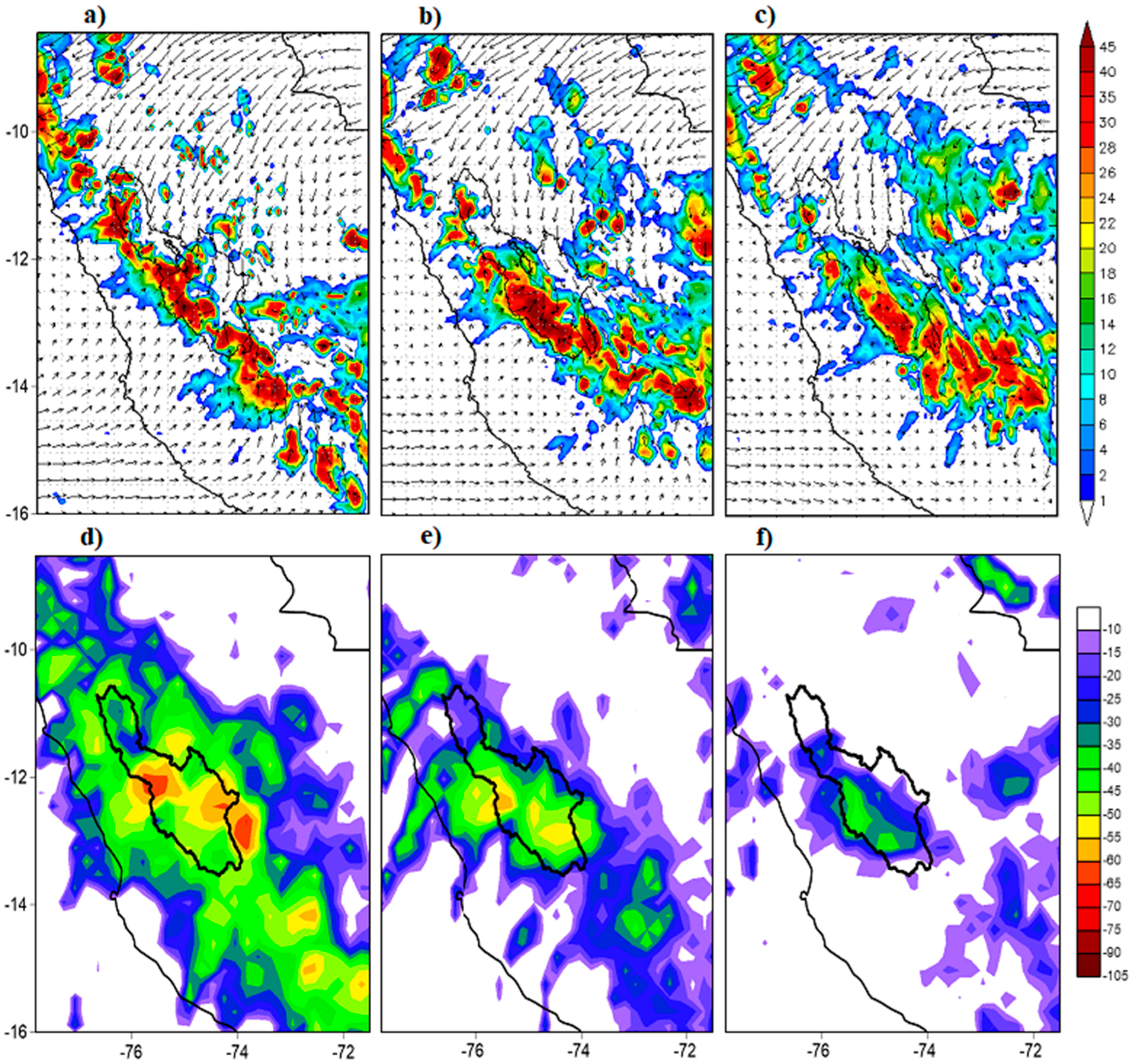
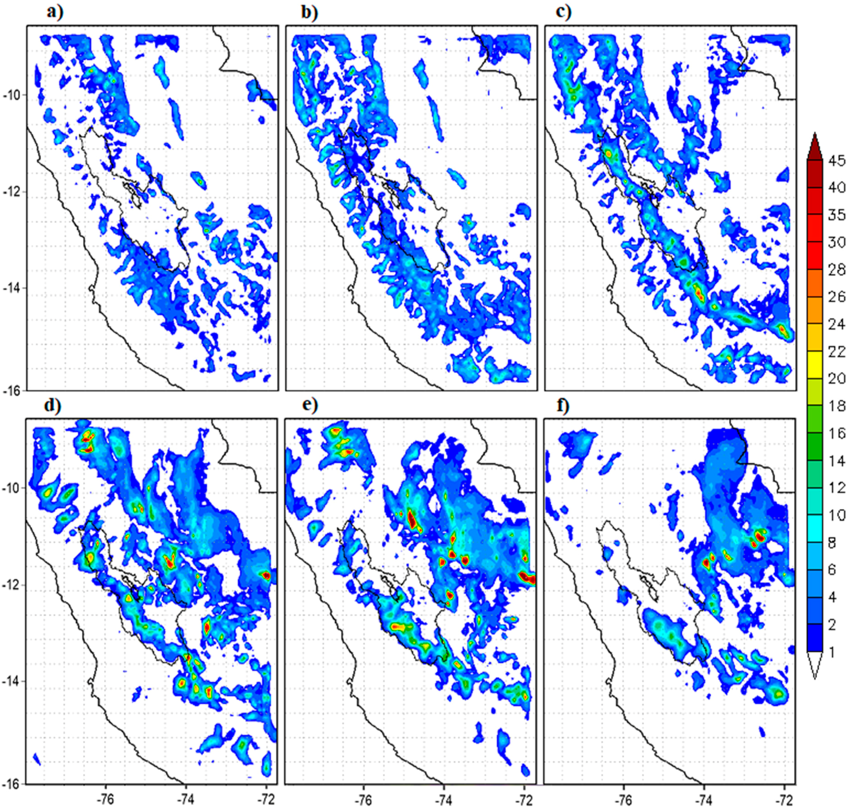
Table 3 shows the statistics of the verification exercise conducted to obtain the parameters B, RMSE, and MAE for the four simulated domains. It can be seen that the model underestimates precipitation in general with all domains, with the largest being negative B of −11.74 mm/day, domain (D3), although in general there is no great difference between the results of the domains except domain D1, of 18 km. It is striking that this domain is the one with the smallest errors—however, in a general verification to evaluate the sensitivity of the model to physical schemes, ref. [17] showed that the resolution domain of 18 km was the one that produced the most precipitation, thus overestimating the recorded rainfall values. It can thus be deduced that in these cases of significant precipitation, this domain (this resolution) is closest to the extreme values. Here, we cannot rule out the fact that the used verification method forces the model to be more precise in the higher resolution domains, which puts them at a disadvantage in relation to the lower resolution domains. In general, the model underestimates approximately between 50% and 60%.
Figure 12 shows the spatial distribution of bias (% of underestimation) for results with domains of 18, 6, 3, and 0.75 km of resolution, with the peculiarity that the 0.75 km domain only covers the area of the Mantaro Valley. In general, in a, b, and c it is observed that the model underestimates the precipitation mainly in the southern half of the basin, precisely where the accumulated ones (as an average) are more significant. In the case of the 0.75 km domain, there are no clear trends in the distribution of B. Notice that domain D4 includes only 7 stations.
Thus, it can be tentatively concluded that WRF underestimates the accumulated precipitation in 24 h for a forecast horizon of up to 36 h, while previous studies show that the model generally overestimates the accumulated precipitation in the region [15,17]. To address this problem, the special experiment mentioned above was conducted. The results (Figure 13) show that when rainfall is greater than approximately 11 mm, the model shows a tendency to underestimate it, as shown by the second-order fit curve (red line in the figure). This is also consistent with Figure 14, which shows that there is registered rainfall above 12 mm for approximately 95% of cases of extreme rainfall. It can be noticed in the Figure that from 28 mm onwards, the bars practically do not grow, which in agreement with Figure 5, showing that precipitation events with rainfall values above this threshold are atypical.

3.4. Case Studies

Two case studies were investigated to explore the processes leading to the significant rainfall underestimations observed in the model simulations, which were in the order of 60% and 82.7% for the cases of 2 February 2011 and 22 March 2009, respectively. The results in both cases will be shown for D2.
In the Case of 2 February 2011, Figure 15 shows values of relative humidity, water-vapor mixing ratio, and wind in the 700–500 hPa layer. It is possible to observe relative humidity values above 70% over the entire territory at both 07 and 13 LST, and moisture transport in the middle troposphere from the Amazon, where values of mixing ratio between 5 and 8 g/kg are observed. Notice how at 13 LST, the water-vapor content over the basin is higher than that which existed at 7 LST, while the relative humidity, though normal, decreased towards midday.
Figure 16 shows the corresponding vertical velocity field averaged over the 600–400 hPa layer and extended into overnight hours. It shows upward motion in the western sector of the Mantaro basin, which increases towards 19 and 22 LST. The ascent encompasses large areas of the Mantaro basin and a large part of the Peruvian Andes range and Amazonia during the entire period.
Corresponding to this, the model max-reflectivity values (it is the variable for equivalent radar reflectivity in the model) also increase after 16 LST, initially in the western sector of the basin and gradually along the mountain range and towards the Amazon, remaining until 04 LST the next day (Figure 17 and Figure 18). This means that although the vertical velocity decreases in the early hours of the morning, the convective cloudiness remains over the region.
Note that in Figure 17 and Figure 18, the highest reflectivity initially develops in the southwest sector of the basin with punctual values approximately up to 30 dbz. It then extends over the mountain range during the afternoon and into the Amazon during the night, reaching values above 35 dbz and gradually decreasing in the northern half of the basin. However, the GOES images show very cold brightness temperatures to the east of the Mantaro basin (not reflected by the model), which gradually approach the basin during the afternoon and are later mixed with the convective lines formed in the vicinity of the basin. The key point is that the model manages to accurately describe the formation of convective clouds over the basin, conditioned by the convergence of easterly and westerly winds in the middle troposphere over the region. However, it does not reproduce early convection at Amazonia, whose propagation towards the basin is assumed to be essential to sustain the large values of accumulated precipitation observed in the region.
As expected, the spatial distribution of the rainfall field of the model (Figure 19) corresponds adequately with the fields of vertical velocity (Figure 16) and maximum reflectivity.
In summary, the underestimation of the model in this case could be a consequence, among other things, of not being able to detect the precipitation areas that originated in the eastern sector of the basin and later providing moisture and vertical motions, resulting in afternoon convection in the Mantaro basin. It may also be related to the fact that the microphysical scheme does not generate enough precipitation, though this requires additional testing.
In the second case (22 March 2009), of which figures are not shown, the results obtained were similar to the previous case. An area with significant brightness temperatures along the ridge in the western sector of the basin could be seen from GOES images, and as in the previous case, convective cells could be observed in the Amazonia from the early hours, which the model was unable to resolve. The results of both case studies suggest that underestimation is partly tied to limitations of the model in resolving Amazonian convection in the early morning hours, apparently related to larger-scale or synoptic processes. Another influential factor could be the mesoscale conditions, which, although the model describes it quite accurately, might not be precise enough to generate vertical movements capable of producing convection and associated precipitation. A third element could be the microphysical scheme and its ability to generate correct accumulated precipitation in extreme events.
The obtained results are consistent with studies conducted in other similar regions. For example, Orr et al. [25] studied the sensitivity of WRF to different parameterization schemes of cloud microphysics when simulating the summer monsoon in Langtang Valley, in the Himalayas. They showed that the parametrization schemes underestimated observed rainfall accumulations, although the forecast horizon may have also influenced this to a certain extent. In that case, the best results were obtained with Morrison’s microphysics scheme, the same one used in the present work.
On the other hand, another study analyzed the sensitivity of the model to microphysics [26], based on the study of a convective storm over the Himalayas (where the comparison was made using data from TRMM and “in situ” observations), and showed a negative bias of the model in all cases. In this case, Morrison’s scheme was also the closest to the observed values.
However, although Mercader et al. [12] has already obtained that for point verification though with different parameterization schemes, WRF is not reliable in precipitation forecasting when accumulations are above the threshold of approximately 10 mm. For this, they used the Fractions Skill Score (FSS) developed in [44].
In a different study [45], sensitivity experiments were carried out with the combination of two cloud clusters and three microphysical schemes for heavy rain that occurred between 28 and 30 May 2010 on the coast of Guyana, which resulted in large differences in the simulations of intense precipitation events between the cumulus schemes, despite using the same initial and contour conditions and model configuration. In general, the model underestimated the level of precipitation. Authors in another study [46] affirm that WRF can be used satisfactorily for weather prediction, but not for simulating precipitation in areas with complex topography, where it shows problems in forecasting rain events in the mountainous terrain of Chile and foothills, where some of the main cities are and where intense rain takes place.
Thus, despite the fact that other studies have shown that WRF overestimates precipitation in this region, the model presents a negative bias for extreme rainfall events. This is consistent with other results for mountain ranges, particularly in the Himalayas and Chilean Andes.

4. Conclusions

This study evaluated the ability of the Weather Research and Forecasting model to forecast extreme short-term rainfall in the Mantaro Basin, in the Peruvian central Andes. Based on the classification of extreme rainfall adopted by SENAMHI, 40 events were selected from observations collected during the period of 2009–2012. WRF-model simulations were carried out using 4 nested domains with horizontal resolutions of 18, 6, 3, and 0.75 km. The selected parametrization schemes included the Grell-Freitas scheme for cumulus, Morrison for microphysics, and Yonsei University for the boundary layer. Point verification was conducted using simple statistics to compare model rainfall to data collected by the SENAMHI observation network. Additionally, the distribution of the model rainfall bias was explored. Two case studies were then analyzed to investigate the processes that may lead to these events in more detail.
Of the selected extreme events, 8 cases were distributed in January, February, and April; 6 in December and March; and 4 in November. Events with rainfall greater than 27 mm were considered atypical, suggesting that the distribution of the series was asymmetric. The spatial distribution of the average and maximum observed rainfall accumulations during the events showed that the highest intensities were concentrated towards the southern half of the basin.
Synoptic analysis of the extreme-event composites suggested that factors associated with heavy rainfall in the Mantaro basin include: (i) moist inflow from the Amazon in the mid-troposphere, characterized by an enhanced northeasterly wind component in southern and central Peru; (ii) ventilation in the northern flank of the subtropical upper ridge or Bolivian high; and (iii) low pressures in the low–mid troposphere, which enhance diurnal circulations and convergence in the Andean boundary layer.
Analysis of the considered statistical indicators indicated that the bias of the model was negative for extreme precipitation events, as the model underestimated precipitation by ~50% and 60% during the selected extreme event cases. In this sense, the complementary experiment that described the relation between the biases and the observed rainfall accumulations showed that the model began to underestimate rainfall when accumulations exceeded approximately 11 mm. Of the studied cases, more than 95% recorded an average rainfall above 12 mm. In general, the model underestimation is greater in the southern and western sector of the basin and in the stations located on the mountain range.
The case studies suggest that one of the causes of rainfall underestimation relates to the inability of the model to generate early-morning convection in the upstream Amazon region, which is an issue apparently related to larger-scale or synoptic processes. Another influential factor is that vertical velocities produced by the model are not sufficiently precise enough to generate the associated cloudiness and precipitation. Another element worth exploring is the ability of the microphysical scheme to generate precipitation totals large enough to qualify as extreme events in the Mantaro basin.

Author Contributions

A.M. conceived the study, performed the WRF simulations and partially processed output files of WRF and GOES information, wrote the main body of the article; J.G. analyzed Section 3.2 and Section 3.4; A.H. prepared and reviewed the data of extreme rainfall; R.E. and S.K. partially processed output information of WRF; E.V. partially processed GOES information; D.M.-C. collaborated with the writing of the article and its general revision in English, Y.S. general coordinator of the project, he made the final review of work.

Funding

This research was funded by FONDECYT, CONCYTEC, Peru (grants 010-2017-FONDECYT).

Acknowledgments

Present study comes under the project “MAGNET-IGP: Strengthening the research line in physics and microphysics of the atmosphere (Agreement N° 010-2017-FONDECYT)”. We would like to thank the FONDECYT, CONCYTEC, Peru, for financial support and Inter-American Institute for Cooperation on Agriculture (IICA) for administrative support. This work was done using computational resources, HPC-Linux Cluster, from Laboratorio de Dinámica de Fluidos Geofísicos Computacionales at Instituto Geofísico del Perú (grants 101-2014-FONDECYT, SPIRALES2012 IRD-IGP, Manglares IGP-IDRC, PP068 program. We would also like to thank NCEP for FNL analysis data and SENAMHI for observational precipitation data.

Conflicts of Interest

The authors declare no conflict of interest.

References

  1. Silva, Y.; Takahashi, K.; Chávez, R. Dry and wet rainy seasons in the Mantaro river basin (Central Peruvian Andes). Adv. Geosci. 2008, 14, 261–264. [Google Scholar] [CrossRef]
  2. Aceituno, P. On the functioning of the Southern Oscillation in the South American. sector. Part II. Upper-air circulation. J. Clim. 1989, 4, 341–355. [Google Scholar] [CrossRef]
  3. Vuille, M.; Kaser, G.; Juen, I. Glacier mass balance variability in the Cordillera Blanca, Peru and its relationship with climate and the large-scale circulation. Glob. Planet. Chang. 2008, 62, 14–28. [Google Scholar] [CrossRef]
  4. Garreaud, R. The Andes climate and weather. Adv. Geosc. 2009, 22, 3–11. [Google Scholar] [CrossRef] [Green Version]
  5. Martínez, A.G.; Núñez, E.; Silva, Y. Vulnerability and adaptation to climate change in the Peruvian Central Andes. In Proceedings of the International Conference on Southern Hemisphere Meteorology and Oceanography (ICSHMO), Foz do Iguacu, Brazil, 24–28 April 2006; pp. 297–305. [Google Scholar]
  6. Armengot-Serrano, R. Las precipitaciones extraordinarias. Atl. Clim. Valencia Collecció Territori. 1994, 4, 98–99. [Google Scholar]
  7. Martín-Vide, J. Spatial distribution of a daily precipitation concentration index in peninsular Spain. Int. J. Climatol. 2004, 24, 959–971. [Google Scholar] [CrossRef] [Green Version]
  8. Moncho, R.; Belda, F.; Caselles, V. Climatic study of the exponent n of the IDF curves of the Iberian Peninsula. Tethys 2009, 6, 3–14. [Google Scholar] [CrossRef]
  9. Harnack, R.P.; Apffel, K.; Cermak, J.R. Heavy precipitation events in New Jersey: Attendant upper-air conditions. Weather Forecast. 1999, 14, 933–954. [Google Scholar] [CrossRef]
  10. Alfaro, L. Estimación de Umbrales de Precipitaciones Extremas Para la Emisión de Avisos Meteorológicos. 2014. Nota Técnica 001-SENAMHI-DGM. Available online: https://issuu.com/senamhi_peru/docs/nota_t__cnica_001-_2014_umbrales_de (accessed on 7 June 2018). (In Spanish).
  11. Skamarock, W.; Klemp, J.; Dudhia, J. A Description of the Advanced Research WRF Version 3; NCAR Technical Note, NCAR/TN-468+STR; National Center for Atmospheric Research (NCAR), Mesoscale and Microscale Meteorology Division: Boulder, CO, USA, 2008. [Google Scholar]
  12. Mercader, J.; Codina, B.; Sairouni, A.; Cunillera, J. Resultados del modelo meteorológico WRF-ARW sobre Cataluña, utilizando diferentes parametrizaciones de la convección y la microfísica de nubes. Tethys 2010, 7, 77–89. (In Spanish) [Google Scholar] [CrossRef]
  13. Wardah, T.; Kamil, A.A.; Sahol Hamid, A.B.; Maisarah, W.W.I. Quantitative Precipitation Forecast using MM5 and WRF models for Kelantan River Basin. Int. J. Geol. Environ. Eng. 2011, 5, 712–716. [Google Scholar]
  14. Joon-Bum, J.; Sangil, K. Sensitivity Study on High-Resolution WRF Precipitation Forecast for a Heavy Rainfall Event. Atmosphere 2017, 8, 96. [Google Scholar] [CrossRef]
  15. Junquas, C.; Takahashi, K.; Condom, T.; Espinosa, J.-C.; Chavez, S.; Sicart, J.-E.; Lebel, T. Understanding the influence of orography on the precipitation diurnal cycle and the associated atmospheric processes in the central Andes. Clim. Dyn. 2017, 1–23. [Google Scholar] [CrossRef]
  16. Chawla, I.; Osuri, K.; Mujumdar, P.; Niyogi, D. Assessment of the Weather Research and Forecasting (WRF) model for simulation of extreme rainfall events in the upper Ganga Basin. Hydrol. Earth Syst. Sci. 2018, 22, 1095–1117. [Google Scholar] [CrossRef] [Green Version]
  17. Moya, A.S.; Martínez-Castro, D.; Flores, J.L.; Silva, Y. Sensitivity Study on the Influence of Parameterization Schemes in WRF_ARW Model on Short- and Medium-Range Precipitation Forecasts in the Central Andes of Peru. Adv. Meteorol. 2018. [Google Scholar] [CrossRef]
  18. Bischoff, S.A.; Vargas, W.M. The 500 and 1000 hPa weather type circulations and their relationship with some extreme climatic conditions over southern South America. Int. J. Clim. 2003, 23, 541–556. [Google Scholar] [CrossRef] [Green Version]
  19. Bischoff, S.A.; Vargas, W.M. Climatic properties of the daily 500 hPa circulation ECWMF reanalysis data over southern South America during 1980–1988. Meteorologica 2006, 23, 3–12. [Google Scholar]
  20. Compagnucci, R.H.; Salles, M.A. Surface pressure patterns during the year over southern South America. Int. J. Clim. 1997, 17, 635–653. [Google Scholar] [CrossRef]
  21. Kalnay, E.M.; Kanamitsu, R.; Kistler, W.; Collins, D.; Deaven, L.; Gandin, M.; Iredell, S.; Saha, G.; White, J.; Woollen, Y.; et al. The NCEP/NCAR 40-Year Reanalysis Project. Bull. Am. Meteorol. Soc. 1996, 77, 437–471. [Google Scholar] [CrossRef] [Green Version]
  22. Rodriguez, E.; Morris, S.C.; Belz, J.E. A Global Assessment of the SRTM Performance. Photogramm. Eng. Remote Sens. 2006, 3, 249–260. [Google Scholar] [CrossRef]
  23. Farr, T.G.; Rosen, P.A.; Caro, E.; Crippen, R.; Riley, D.; Hensley, S.; Kobrick, M.; Paller, M.; Rodríguez, E.; Ladislav, R.; et al. The Shuttle Radar Topography Mission. Rev. Geophys. 2007. [Google Scholar] [CrossRef]
  24. González, Y.; Mesquita, M. Numerical Simulations of the 1 May 2012 Deep Convection Event over Cuba: Sensitivity to Cumulus and Microphysical Schemes in a High-Resolution Model. Adv. Meteorol. 2015. [Google Scholar] [CrossRef]
  25. Orr, A.; Listowski, C.; Cottet, M.; Collier, E.; Immerzeel, W.; Deb, P.; Bannister, D. Sensitivity of simulated summer monsoonal precipitation in Langtang Valley, Himalaya, to cloud microphysics schemes in WRF. J. Geophys. Res. 2017, 122, 6298–6318. [Google Scholar] [CrossRef] [Green Version]
  26. Shrestha, R.K.; Connolly, P.J.; Gallagher, M.W. Sensitivity of WRF cloud microphysics to simulations of a convective storm over the Nepal Himalayas. Open Atmos. Sci. J. 2017, 11, 29–43. [Google Scholar] [CrossRef]
  27. Rajeevan, M.; Kesarkar, A.; Thampi, S.B.; Rao, T.N.; Radhakrishna, B.; Rajasekhar, M. Sensitivity of WRF cloud microphysics to simulations of a severe thunderstorm event over Southeast India. Ann. Geophys. 2010, 28, 603–619. [Google Scholar] [CrossRef] [Green Version]
  28. Morrison, H.; Thompson, G.; Tatarskii, V. Impact of cloud microphysics on the development of trailing stratiform precipitation in a simulated squall line: Comparison of one- and two-moment schemes. Mon. Weather Rev. 2009, 137, 991–1007. [Google Scholar] [CrossRef]
  29. Hong, S.-Y.; Noh, Y.; Dudhia, J. A new vertical diffusion package with an explicit treatment of entrainment processes. Mon. Weather Rev. 2006, 134, 2318–2341. [Google Scholar] [CrossRef]
  30. Paulson, C.A. The mathematical representation of wind speed and temperature profiles in the unstable atmospheric surface layerm. J. Appl. Meteorol. 1970, 9, 857–861. [Google Scholar] [CrossRef]
  31. Dyer, A.J.; Hicks, B.B. Flux–gradient relationships in the constant fluxlayer. Q. J. R. Meteorol. Soc. 1970, 96, 715–721. [Google Scholar] [CrossRef]
  32. Webb, E.K. Profile relationships: The log-linear range, and extension to strong stability. Q. J. R. Meteorol. Soc. 1970, 96, 67–90. [Google Scholar] [CrossRef]
  33. Zhang, D.; Anthes, R.A. A high-resolution model of the planetary boundary layer—Sensitivity tests and comparisons with SESAME-79 data. J. Appl. Meteorol. 1982, 21, 1594–1609. [Google Scholar] [CrossRef]
  34. Beljaars, A.C.M. The parameterization of surface fluxes in large-scale models under free convection. Q. J. R. Meteorol. Soc. 1994, 12, 255–270. [Google Scholar]
  35. Iacono, M.J.; Delamere, J.S.; Mlawer, E.J.; Shephard, M.W.; Clough, S.A.; Collins, W.D. Radiative forcing by long-lived greenhouse gases: Calculations with the AER radiative transfer models. J. Geophys. Res. 2008, 113, D13103. [Google Scholar] [CrossRef]
  36. Grell, G.A.; Freitas, S.R. A scale and aerosol aware stochastic convective parameterization for weather and air quality modeling. Atmos. Chem. Phys. 2014, 14, 5233–5250. [Google Scholar] [CrossRef] [Green Version]
  37. Tewari, M.; Chen, F.; Wang, W.; Dudhia, J.; LeMone, M.A.; Mitchell, K.; Ek, M.; Gayno, G.; Wegiel, J.; Cuenca, R.H. Implementation and verification of the unified NOAH land surface model in the WRF model. In Proceedings of the 20th Conference on Weather Analysis and Forecasting, 16th Conference on Numerical Weather Prediction, Seattle, WA, USA, 14 January 2004; pp. 11–15. [Google Scholar]
  38. Weisman, M.L.; Davis, C.; Wang, W.; Manning, K.W.; Klemp, J.B. Experience with 0–36 h explicit convective forecast with the WRF-ARW model. Weather Forecast. 2008, 407–437. [Google Scholar] [CrossRef]
  39. Molinari, J.; Dudek, M. Parametrization of convective precipitacion in mesoscale numerical models: A critical review. Mon. Weather Rev. 1992, 120, 326–344. [Google Scholar] [CrossRef]
  40. Belair, S.; Mailhot, J. Impact of horizontal resolution on the numerical simulation of a midlatitude squall line: Implicit versus explicit condensation. Mon. Weather Rev. 2001, 129, 2362–2375. [Google Scholar] [CrossRef]
  41. Done, J.; Christopher, A.D.; Weisman, M.L. The next generation of nwp: Explicit forecasts of convection using the weather research and forecast (WRF) model. Atmos. Sci. Lett. 2004, 5, 110–117. [Google Scholar] [CrossRef]
  42. Cressman, G.P. An operational objective analysis system. Mon. Weather Rev. 1959, 87, 367–374. [Google Scholar] [CrossRef]
  43. Garreaud, R.; Vuille, M.; Clement, A.C. The climate of the Altiplano: Observed current conditions and mechanisms of past changes. Paleogeogr. Paleoclimatol. Paleoecol. 2003, 194, 5–22. [Google Scholar] [CrossRef]
  44. Roberts, N.M.; Lean, H. Scale-Selective Verification of Rainfall Accumulations from High-Resolution Forecasts of Convective Events. Mon. Weather Rev. 2008, 136, 78–97. [Google Scholar] [CrossRef]
  45. Rama Rao, Y.V.; Alves, L.; Seulall, B.; Mitchell, Z.; Samaroo, K.; Cummings, G. Evaluation of the weather research and forecasting (WRF) model over Guyana. Nat. Hazards 2012, 61, 1243–1261. [Google Scholar] [CrossRef]
  46. Yáñez-Morroni, G.; Gironás, L.; Caneo, M.; Delgado, R.; Garreaud, R. Using the Weather Research and Forecasting (WRF) Model for Precipitation Forecasting in an Andean Region with Complex Topography. Atmosphere 2018, 9, 304. [Google Scholar] [CrossRef]
Figure 1. Spatial distribution of the observation network stations.
Atmosphere 09 00362 g001
Figure 2. Model domains used in the simulations. Terrain elevation is indicated with color shades in meters above sea level. In the 3 largest domains, the black contour indicates the limits of the Mantaro Basin. In D4, black contour indicates Mantaro Valley.
Atmosphere 09 00362 g002
Figure 3. Monthly distribution of the 40 extreme event cases considered.
Atmosphere 09 00362 g003
Figure 4. Monthly distribution of the maximum 24 h accumulated precipitation (mm) at the given station among all the studied events.
Atmosphere 09 00362 g004
Figure 5. Histogram (a) and box diagram (b) of the network-averaged extreme rainfall observation series considered in the investigation. In the box diagram, the whiskers correspond to maximum and minimum values, excluding outliers. The box shows the standard deviation and the line is the mean value.
Atmosphere 09 00362 g005
Figure 6. Spatial distribution of the mean (a) and maximum (b) accumulated rainfall observed in mm/day.
Atmosphere 09 00362 g006
Figure 7. Geopotential height (m) composite charts for 500 hPa (top) and 700 hPa (bottom) averaged over the rainy seasons of 1981–2017 (a,d); the 40 extreme rainfall event cases (b,e) and their difference (c,f) to highlight deviations from the rainy season climatology.
Atmosphere 09 00362 g007
Figure 8. Composite wind fields averaged over the 40 extreme rainfall event cases for 700 hPa (a) and 500 hPa (b) in m s−1.
Atmosphere 09 00362 g008
Figure 9. 500–700 hPa layer relative humidity averaged over the rainy seasons of 1981–2017 (a); the 40 extreme rainfall event cases (b) and their difference (c) to highlight deviations from the rainy season climatology.
Atmosphere 09 00362 g009
Figure 10. Average geopotential height of 200 hPa of the rainy period from 1981 to 2017 (a) and the 40 extreme rainfall events (b) considered in m.
Atmosphere 09 00362 g010
Figure 11. Average 200 hPa wind field (m s−1) and divergence (s−1 × 10⁶) of the 40 cases.
Atmosphere 09 00362 g011
Figure 12. Spatial distribution of bias (%) for results with domains D1 (a), D2 (b), D3 (c), and D4 (d). The numbers above the circles indicate the percentage of underestimation.
Atmosphere 09 00362 g012
Figure 13. Bias curve of the Weather Research and Forecasting (WRF) model relative to observed precipitation. The red line shows its second-order polynomial fit curve.
Atmosphere 09 00362 g013
Figure 14. Cumulative frequency histogram of cases of extreme precipitation relative to recorded rainfall.
Atmosphere 09 00362 g014
Figure 15. WRF-simulated relative humidity (%) (top) and water-vapor mixing ratio (bottom) (g/kg), averaged over the 700–500 hPa layer at 07 LST (Local Standard Time) (a,c) and 13 LST (b,d) of 2 February 2011.
Atmosphere 09 00362 g015
Figure 16. WRF-simulated average vertical velocity in the 600–400 hPa layer (m s−1) over the region at 13 LST, 16 LST, 19 LST, and 22 LST of 2 February 2011 (ad); and at 01 LST and 04 LST (e,f) of 3 February 2011.
Atmosphere 09 00362 g016
Figure 17. WRF-simulated maximum reflectivity (dBZ) and wind vector in 550 hPa (top); and corresponding GOES brightness temperature (°C) (bottom) over the region at 13 LST (a,d), 16 LST (b,e), and 19 LST (c,f) of 2 February 2011.
Atmosphere 09 00362 g017
Figure 18. WRF-simulated maximum reflectivity (dBZ) and wind vector in 550 hPa (top); and corresponding GOES brightness temperature (°C) (bottom) at 22 LST of 2 February 2011 (a,d); and at 01 LST (b,e) and 04 LST (c,f) of 3 February 2011.
Atmosphere 09 00362 g018
Figure 19. WRF-simulated precipitation (mm/3 h) at 13 LST, 16 LST, 19 LST, and 22 LST of 2 February (ad); and 01 LST and 04 LST (e,f) of 3 February 2011.
Atmosphere 09 00362 g019
Table 1. Dates of cases of extreme rainfall selected for the study.
Fechas
7 April 20094 April 201017 February 201110 December 2011
8 April 20094 December 201012 March 201114 December 2011
11 April 20097 January 201113 March 201125 December 2011
22 November 200914 January 201121 March 20116 February 2012
28 November 200922 January 201129 March 201128 February 2012
17 December 200925 January 20111 April 20114 April 2012
10 January 201029 January 20115 April 201122 April 2012
7 April 20094 April 201017 February 201110 December 2011
8 April 20094 December 201012 March 201114 December 2011
11 April 20097 January 201113 March 201125 December 2011
Table 2. Main characteristics of the domains and initial and boundary conditions.
CharacteristicsDomain 1
(D1)
Domain 2
(D2)
Domain 3
(D3)
Domain 4
(D4)
Central pointLat: 10° S
Lon: 75° W
Lat: 12.25819° S
Lon: 74.8356° W
Lat: 12.36526° S
Lon: 75.0274° W
Lat: 11.96349° S
Lon: 75.3562° W
Horizontal step18 km6 km3 km0.75 km
Dimensions (XYZ)115 × 140 × 28115 × 142 × 28127 × 163 × 28113 × 121 × 28
Time step90 s36 s18 s4 s
Initial and border conditionsFNL (1°)Simulation of domain 1Simulation of domain 2Simulation of domain 3
Table 3. Statistics of verification for the 4 simulated domains, average of all stations. In parentheses are the percentages of underestimation.
StatisticsD1D2D3D4
B (mm/day)−9.40 (49.5%)−11.07 (58.3%)−11.74 (61.8%)−11.71 (61.6%)
RMSE (mm/day)11.6813.1412.8612.60
MAE (mm/day)13.9515.1415.0714.51

