Design of an MPPT Technique for the Indirect Measurement of the Open-Circuit Voltage Applied to Thermoelectric Generators

Abstract

This paper presents the design of a maximum power point-tracking (MPPT) technique for DC–DC converters that are used in energy-harvesting systems based on thermoelectric generators. This technique is based on the analysis of the characteristics of the converter to measure the open-circuit voltage indirectly. The main contribution of this article is that the algorithm measures the voltage at the maximum power point without the need to disconnect the source of the circuit, as happens when the fractional open-circuit voltage (FOCV) technique is used. The algorithm is based on a predetermined initial duty cycle, which is applied to the circuit, and the input voltage and input current are read. With these values, the open-circuit voltage and short-circuit current are calculated with equations obtained from the circuit. Then, it calculates the duty cycle at the maximum power point and applies it to the circuit. If this duty cycle does not obtain the maximum power from the circuit, the algorithm starts a second stage based on fuzzy logic to calculate an increase or decrease in the duty cycle. The designed technique was evaluated using a topology based on a DC–DC flyback converter variant and was compared with the P&O technique and obtained better results. The designed technique provides between 3.9% and 5.6% more power to the load than the P&O technique in a 20 W system.

1. Introduction

A thermoelectric (TE) module is a P–N junction of two different semiconductors. When a set of these junctions is electrically connected in series and thermally in parallel [1], a device called a thermoelectric generator (TEG) is formed, which directly converts the thermal energy into electricity, exploiting the Seebeck effect [2]. A thermoelectric generator has low efficiency (approximately 5%) when compared to a photovoltaic panel (21%), which is why its use in recent years has been only for military, medical and aerospace applications [3]. However, progress in materials studies has allowed improvement of the efficiency of said devices and the use of renewable energies, and the increase in the cost of production of electrical energy has increased interest in applications of this field, using the TEGs as a viable source of electricity [4].

The main disadvantage of a thermoelectric generator is its high internal resistance, which can be neglected when there are large-scale TEG applications (for example in kilowatt power systems) but not when there are low-power applications (for example in power systems of 100 watts or less). When there is a difference in temperature between the hot and cold faces of the TEG, a change in its internal resistance occurs, which causes a loss of energy in the system [5]. To help minimize these losses in energy harvesting, maximum power point-tracking (MPPT) control systems are used and implemented, especially when the system has a vast temperature distribution. This MPPT control can increase the efficiency of the system if it is combined with the use of the appropriate converter for each application.

Due to the nature of TEGs, they cannot be directly connected to the application, so the use of a DC–DC converter is needed to improve the efficiency of these systems, such as photovoltaic systems [6,7]. The change in temperature affects the output power of these devices [8], so it is necessary to use an MPPT system to compensate for these changes in temperature and ensure that the output power is not affected during the dynamic change. There are many studies that have been done to improve the efficiency of TEGs by modifying the main components that comprise it or using new semiconductors; however, the efficiency of these is still low [9]. Recently, there have been many works related to applications between TEGs and heat exchangers for the recovery of residual heat from thermal applications to improve the performance of devices [10].

Some uses of TEGs have been reported in aerospace applications [11], automotive systems [12,13], ecological stoves [1,14], battery charging [15,16], industrial processes [17], portable thermoelectric generators for power supply of ultra-low-power sensors [18], device detection in remote pipelines [19], car exhaust gas systems [20] and other fields. Recent advances in semiconductor materials with excellent thermoelectric performance [19] greatly promote the use of TEGs in different applications for the recovery of waste heat from power plants, automobiles, industrial boilers, foundry furnaces, frying machines and other industrial heat generation processes.

The most used algorithms in power generation systems using thermoelectric generators are Fractional Open-Circuit Voltage (FOCV), Incremental Conductance (IC), Perturb and Observe (P&O) and Fractional Short-Circuit Current (FSCC) [21,22]. P&O is the algorithm that searches for the maximum power point by introducing disturbances in the input voltage [23,24] and the operating point oscillates around the MPP. In this technique, a disturbance is fixed, which is the step between each cycle and determines the magnitude of the disturbance that will be generated according to the change in the duty cycle. On the other hand, the IC algorithm is based on the change in power divided by the change in voltage, which is equal to zero at the MPP point [22,25] and the step size should be smaller than the error margin. Since both algorithms work with perturbations, they need to have a variable step size to minimize the error at the maximum power point [26,27].

The FOCV method uses the quasi-linear relationship that exists between the open-circuit voltage (OCV) and the voltage at the maximum power point ($V_{MPP}$). Similar to the FSCC method, it uses the ratio of the short-circuit current (SCC) to the current at the maximum power point ($I_{MPP}$). For TEGs, the $V_{MPP}$ and $I_{MPP}$ are approximately 50% of the VOC and ISCC, respectively. The operation of these methods is quite good in steady state, but during the measurements of the values mentioned above, there is a loss of energy due to the disconnection of the circuit. The MPPT converter proposed by [28] is based on the OCV algorithm, but the disconnection between the converter and the TEG causes voltage spikes in the circuit that directly affect the speed of the program.

In [29], an energy-harvesting system is proposed that has an auxiliary system to mitigate instantaneous consumption peaks that cause low performance in the supply source. This system consists of a battery and a supercapacitor. The battery provides the energy in a stable state and the supercapacitor provides the voltage peaks that are consumed in very short instants of time but with a high demand. The technique used was fuzzy logic in combination with load power tracking (LTP) to control the field bus that feeds the load, so that they take turns and provide the required energy according to the demand of the load. This strategy distributes the energy generated by the source to the load and to the field bus, and has a tracking efficiency with an error range of 3.5% for powers from 2 to 4 watts.

This paper presents the design of a maximum power point-tracking technique based on an indirect measurement of the open-circuit voltage and short-circuit current for reaching the maximum power point in thermoelectric generator applications. In a second stage, the algorithm uses fuzzy logic to determine the near-optimal duty cycle. This paper is organized as follows: Section 2 presents the flow diagram of the proposed technique and explains the analysis of the circuit to determine the equations for the duty cycle in the maximum power point and focuses on the fuzzy logic stage. Section 3 shows the simulation results obtained and finally, in Section 4, the main conclusions of this document are presented.

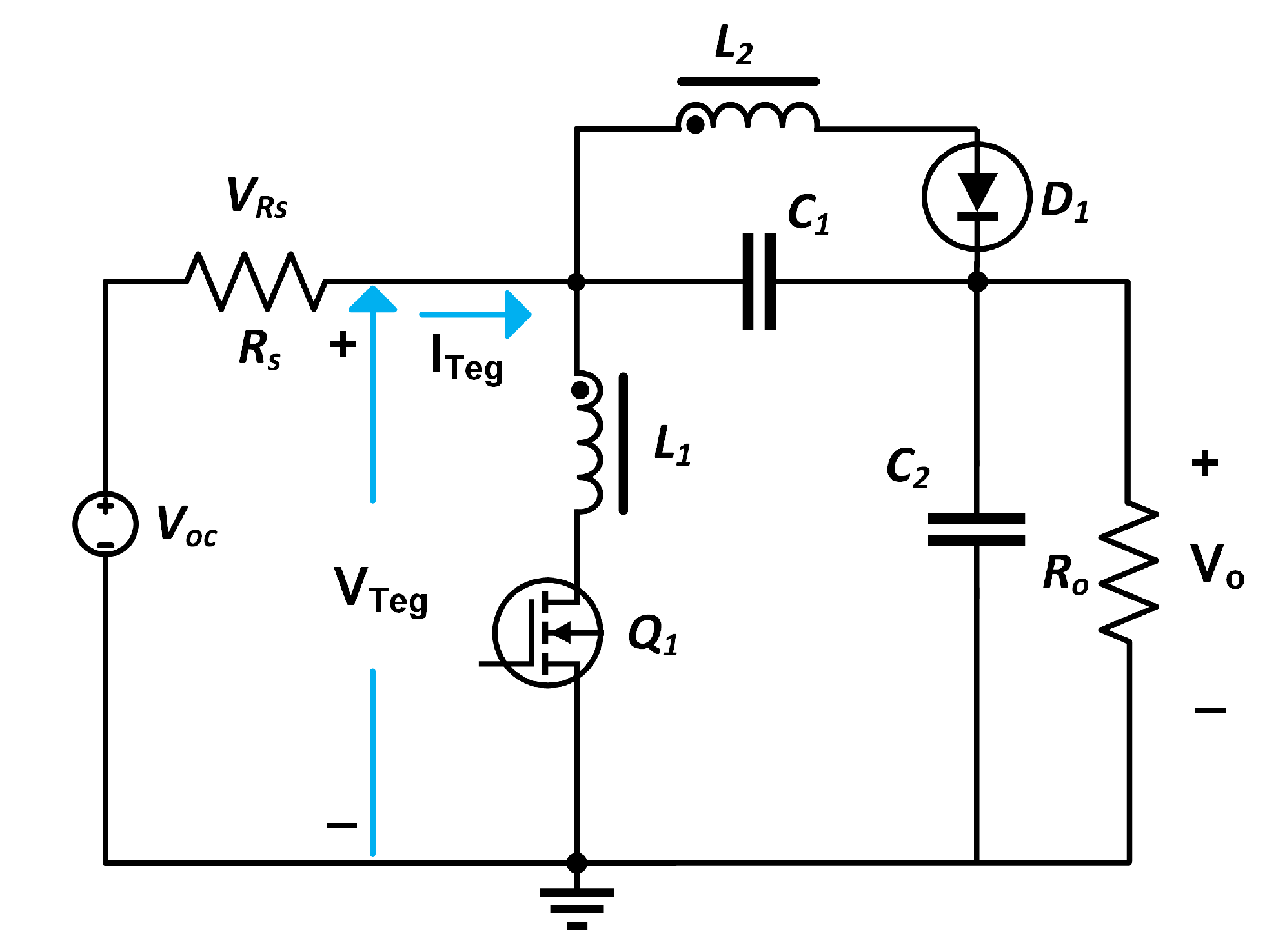
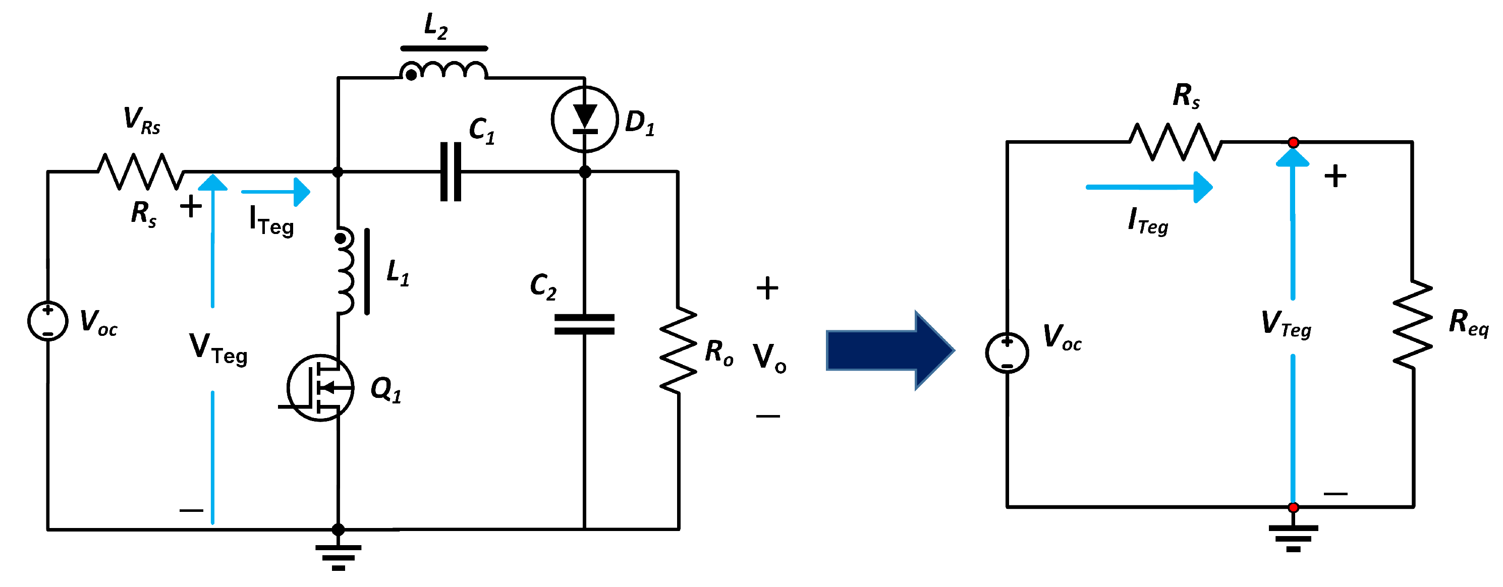
2. Proposed MPPT Control Algorithm

The proposed algorithm is known as IOCV&FL in this paper, and combines two different techniques—the fractional open-circuit voltage and fuzzy logic. The main advantage is the possibility of measurement and calculation of the open-circuit voltage indirectly without the need to disconnect the circuit from the power supply, eliminating the switch used for this. The algorithm finds the relationship between the voltage at the maximum power point and the optimal duty cycle to apply this in the converter. Using an initial duty cycle, the algorithm calculates the optimal duty cycle and if this duty cycle does not extract the maximum power, a second stage starts to find it. This stage uses fuzzy logic and reads the input voltage and input current to recalculate the optimal duty cycle. The flow chart of the proposed maximum power point-tracking algorithm is shown in Figure 1.

The algorithm IOCV&FL is based on a predetermined initial duty cycle $D_1$ that is applied to the circuit, and the input voltage and input current values are read ($V_1$ e $I_1$, respectively). With these values, the slope m is calculated in that point, along with the values of the short-circuit current $I_{sc}$ and the open-circuit voltage $V_{oc}$, the voltage at the maximum power point $V_{MPP}$ and the current at the point of maximum power $I_{MPP}$ are also calculated. With this, the duty cycle at the maximum power point $D_{MPP}$ is calculated. After the first iteration, the new calculated duty cycle is applied, and the response of the circuit is read again, thus obtaining the new one’s voltage and current values in the current state. With these values, the power $P_1$ that could be used in the second part of the algorithm is calculated. After this, the algorithm makes a comparison of the actual voltage with respect to the previous voltage and, if the absolute value of that voltage difference is less than or equal to a certain error 1 $e_1$, it means that the circuit is working at the maximum power point, so the applied duty cycle is optimal and is reapplied to the circuit. Hoping to continue in that range, $D_{old}$ is the duty cycle of the previous iteration.

If the absolute value of the voltage difference is greater than the error 1 $e_1$, then the current values of voltage and current enter the fuzzy rule base, in which an increase or decrease in the duty cycle is calculated $\Delta D$, which is applied to the previous duty cycle, and a new duty cycle is calculated D. This new duty cycle is applied, the circuit voltage and current values are read again, and a new one is calculated power $P_2$, which is the power in the current state. The next step is to make a comparison between this power and the previous power $P_1$. If the absolute value of this difference is less than an error 2 $e_2$, it indicates that the optimal operating point has already been found and therefore this new duty cycle determined by the fuzzy rule base is applied to the circuit again. Otherwise, if the absolute value of the power difference is greater than or equal to the error 2 $e_2$, it returns to the beginning of the algorithm to recalculate new values of the open-circuit voltage and short-circuit current, starting the MPPT control algorithm again.

Equations (1) and (2) show the formulas for the difference between voltages and powers, respectively.

$$\Delta V=V-V_1$$

(1)

$$\Delta P=P_2-P_1$$

(2)

This algorithm has two stages. The first stage is the analysis of the converted used. It is necessary to analyze the characteristics to determine the equations for the open-circuit voltage, short-circuit current, voltage, and current at the maximum power point, and finally the near-optimal duty cycle (duty cycle at the maximum power point). If the first stage does not find the duty cycle in the MPP, the algorithm enters the second stage, in which the duty cycle is located by fuzzy logic.

2.1. Indirect Measurement of the Open-Circuit Voltage

The first stage of the proposed algorithm is the indirect measurement of the open-circuit voltage. To evaluate this technique, a DC–DC converter [30] based on a flyback variant is used. One of the contributions of the article is that it allows the constant flow of energy from the source to the load, since a small part is delivered directly by the TEGs to the load and the other part is processed by the converter to later be delivered to load. The flyback converter with the proposed modification can only raise the voltage, but gains benefits such as eliminating current peaks at the input, with greater stability and reduced stress on converter components. The efficiency reported in the experimental results is 92.65% in an implemented prototype of 18 watts with constant voltage, current, load and duty cycle, without a maximum power point-tracking control system.

The main advantage of this technique is the option to calculate the voltage at the maximum power point ($V_{MPP}$) indirectly without the need to disconnect the power supply from the circuit to sense the open-circuit voltage at any given time, decreasing the components that are needed (eliminating the connection and disconnection MOSFET of the source with the circuit and disabling the control signal of the micro-controller and the power devices that are used for the control of MOSFET), thus reducing power losses in said components. Figure 2 shows the converter used in this paper. $I_{Teg}$ is the input current and $V_{Teg}$ is the input voltage provided by the Teg.

The analysis is started by taking up the equation of the gain of the converter designed in [30] to obtain the TEG voltage ($V_{Teg}$) and current ($I_{Teg}$) equations.

$$M=1+\frac{D}{n(1-D)}$$

(3)

Knowing that the gain is the output voltage ($V_o$) divided by the input voltage ($V_{Teg}$), (3) can be rewritten as follows:

$$\frac{V_o}{V_{Teg}}=1+\frac{D}{n(1-D)}$$

(4)

From the previous equation, we solve for the input voltage, which is the voltage of the TEG:

$$V_{Teg}=\frac{V_o}{1+\frac{D}{n(1-D)}}$$

(5)

To calculate the TEG current ($I_{Teg}$), we start from the equation:

$$P_{Teg}=P_o+P_{fi}-P_{fo}$$

(6)

In Equation (6), $P_{Teg}$ is the power supplied by the TEG, $P_o$ is the output power of the system, $P_{fi}$ is the input power of the converter, and $P_{fo}$ is the output power of this converter. Knowing that the efficiency of the converter is:

$$n_f=\frac{P_{fo}}{P_{fi}}$$

(7)

The ratio of the input power of the converter minus its output power is calculated, as observed in (8).

$$P_{fi}-P_{fo}=\frac{P_{fo}}{n_f}-P_{fo}=P_{fo}\left(\frac{1}{n_f}-1\right)$$

(8)

Substituting (8) in (6), we have the following:

$$P_{Teg}=P_o+P_{fo}\left(\frac{1}{n_f}-1\right)$$

(9)

Describing the above equation as a function of voltage and current, the output power of the converter is equal to the voltage across the inductor $L_2$ ($V_{L_2}$) multiplied by the output current $I_o$.

$$V_{Teg}{I}_{Teg}=V_o{I}_o+V_{L_2}{I}_o\left(\frac{1}{n_f}-1\right)$$

(10)

The voltage across the inductor $L_2$ is calculated as follows:

$$V_{L_2}=V_o-V_{Teg}$$

(11)

Substituting (11) in (10), an equation is obtained that relates the TEG current as a function of the output voltage and the TEG voltage.

$$V_{Teg}{I}_{Teg}=V_o{I}_o+(V_o-V_{Teg})I_o\left(\frac{1}{n_f}-1\right)$$

(12)

From this relationship, the value of the TEG current is solved to obtain its equation.

$$I_{Teg}=I_o\left[1+\frac{1}{n_f}·\frac{D}{n(1-D)}\right]$$

(13)

For a more simplified analysis, the components of the converter plus the load can be seen as a single equivalent resistance, which will be seen by the TEG as the load, as shown in Figure 3, where $R_{eq}$ is the equivalent resistance of the converter and the load together, seen by the TEG. $I_{Teg}$ is the input current and $V_{Teg}$ is the input voltage provided by the Teg.

With the simplified circuit, we have the following relationship:

$$V_{Teg}=R_{eq}{I}_{Teg}$$

(14)

Substituting (5) and (13), the following relationship is obtained:

$$\frac{V_o}{1+\frac{D}{n(1-D)}}=R_{eq}{I}_o\left[1+\frac{1}{n_f}·\frac{D}{n(1-D)}\right]$$

(15)

From the above relationship, the equation of the value of the equivalent resistance seen by the TEG is calculated as a function of the output resistance of the circuit $R_o$ and the duty cycle D.

$$R_{eq}=\frac{R_o}{1+\frac{D}{n(1-D)}\left[1+\frac{1}{n_f}\left(1+\frac{D}{n(1-D)}\right)\right]}$$

(16)

The equivalent input resistance seen by the TEG in the condition of the maximum power point is obtained when the converter is working with the optimal duty cycle ($D_{MPP}$).

$$R_{MPP}=\frac{R_o}{1+\frac{D_{MPP}}{n(1-D_{MPP})}\left[1+\frac{1}{n_f}\left(1+\frac{D_{MPP}}{n(1-D_{MPP})}\right)\right]}$$

(17)

The open-circuit voltage is equal to the sum of the internal resistance voltage ($V_{R_s}$) and the TEG voltage ($V_{Teg}$), which is the total load voltage (which includes the converter and final load resistance).

$$V_{oc}=V_{R_s}+V_{Teg}$$

(18)

From the previous relationship, the voltage in the internal resistance $R_s$ is cleared.

$$R_s{I}_{Teg}=V_{oc}-V_{Teg}$$

(19)

From (19), the value of the TEG current is solved to arrive at the following equation:

$$I_{Teg}=\frac{V_{oc}}{R_s}-\frac{1}{R_s}·V_{Teg}$$

(20)

which is a linear equation of the form $y=mx+b$ where the slope $m=-\frac{1}{R_s}$ and $b=\frac{V_{oc}}{R_s}$.

The open-circuit voltage divided by the internal resistance of the TEG equals the short-circuit current $I_{sc}$. Therefore, the previous equation for a certain point “A” with a voltage value $V_1$ and current $I_1$ is expressed as follows:

$$I_1=m{V}_1+I_{sc}$$

(21)

From here, the value of the short-circuit current is cleared:

$$I_{sc}=I_1-m{V}_1$$

(22)

When the short-circuit current is known, the current at the point of maximum power ($I_{MPP}$) is easily calculated, which is defined as follows, according to [3,31]:

$$I_{MPP}=0.5I_{sc}$$

(23)

Under the open-circuit condition, there is no current flow through the TEG, so (21) looks like this:

$$0=m{V}_{oc}+I_{sc}$$

(24)

Solving for the value of the open-circuit voltage from there:

$$V_{oc}=\frac{I_{sc}}{-m}$$

(25)

Knowing the voltage and current values at a certain point “A”, what remains to be defined is the value of the slope at that point. For this specific case, in which model HZ-9 TEGs from the manufacturer Hi-Z Technology are being used, the voltage–current curve is observed in Figure 4, as well as its line trend expressed in a fourth-order polynomial function. The hot side of the TEG was 210 ${}^{\circ }$C and the cold side was 55.23 ${}^{\circ }$C.

The equation of the trend line (red line) of the V–I curve of the characterized TEGs is the following:

$$I=7.64516\times {10}^{-5}{V}^4-0.00307V^3+0.03314V^2-0.19467V+3.33798$$

(26)

To determine the value of the slope m at any point on the trend line, the derivative of the function is calculated, thus obtaining the equation of the slope that is needed to later calculate the $I_{sc}$ and the $V_{oc}$.

$$m=0.0003058V^3-0.00921V^2+0.06628V-0.19467$$

(27)

Knowing the values of the voltage ($V_1$), current ($I_1$) and the slope (m), the short-circuit current ($I_{sc}$) and the open-circuit voltage ($V_{oc}$), in addition to the voltage ($V_{MPP}$) and the current ($I_{MPP}$) at the maximum power point can be calculated indirectly, without the need to open the circuit and disconnect the converter source to obtain those values.

Returning to (14), an equation is found that relates the voltage of the TEG with the current of this, together with the duty cycle and the final load resistance $R_o$.

$$V_{Teg}=\frac{R_o}{1+\frac{D}{n(1-D)}\left[1+\frac{1}{n_f}\left(1+\frac{D}{n(1-D)}\right)\right]}·I_{Teg}$$

(28)

When the voltage of the TEG is equal to the voltage at the maximum power point and the current of the TEG is equal to the current at the maximum power point, it indicates that the optimum point is being worked on, therefore the applied duty cycle at that time it is equal to the optimal duty cycle ($D_{MPP}$). Then, (28) is rewritten as follows:

$$V_{MPP}=\frac{R_o}{1+\frac{D_{MPP}}{n(1-D_{MPP})}\left[1+\frac{1}{n_f}\left(1+\frac{D_{MPP}}{n(1-D_{MPP})}\right)\right]}·I_{MPP}$$

(29)

In Equation (29), $V_{MPP}=$ voltage at the maximum power point, $I_{MPP}=$ current at the maximum power point, $R_o=$ load resistance, $n=$ transformation ratio of the transformer and $n_f=$ efficiency of the converter and $D_{MPP}=$ duty cycle at maximum power point.

Dividing $\frac{V_1}{V_{MPP}}$ we obtain the following:

$$\frac{V_1}{V_{MPP}}=\frac{\frac{R_o}{1+\frac{D_1}{n(1-D_1)}\left[1+\frac{1}{n_f}\left(1+\frac{D_1}{n(1-D_1)}\right)\right]}·I_1}{\frac{R_o}{1+\frac{D_{MPP}}{n(1-D_{MPP})}\left[1+\frac{1}{n_f}\left(1+\frac{D_{MPP}}{n(1-D_{MPP})}\right)\right]}·I_{MPP}}$$

From the above relationship, a dependence of the duty cycle at the point of maximum power with the previous duty cycle, the voltage, the current, the voltage at the point of maximum power, and the current at the point of maximum power is observed. Therefore, we proceed to clear the value of the duty cycle at the maximum power point ($D_{MPP}$), obtaining the following equation:

$$D_{MPP}=\frac{n·y}{1+n·y}$$

(30)

In Equation (30), n is the transformation ratio of the transformer, “y” is a factor that has the following formula:

$$y=\frac{n_f\left[\sqrt{{\left(1+\frac{1}{n_f}\right)}^2-\frac{4(1-x)}{n_f}}-\left(1+\frac{1}{n_f}\right)\right]}{2}$$

(31)

In the equation described above, $n_f$ is the efficiency of the designed converter and x is a factor that includes the previous duty cycle, voltage and current, the transformer’s transformation ratio, voltage, and current at the point of maximum power, as seen in (32).

$$x=\frac{V_1·I_{MPP}\left[1+\frac{D_1}{n(1-D_1)}\left[1+\frac{1}{n_f}\left(1+\frac{D_1}{n(1-D_1)}\right)\right]\right]}{V_{MPP}·I_1}$$

(32)

The duty cycle obtained $D_{MPP}$ is applied to the circuit to evaluate its response and read the new voltage and current values. With this methodology, is not necessary to disconnect the TEG from the circuit for measuring the open-circuit voltage.

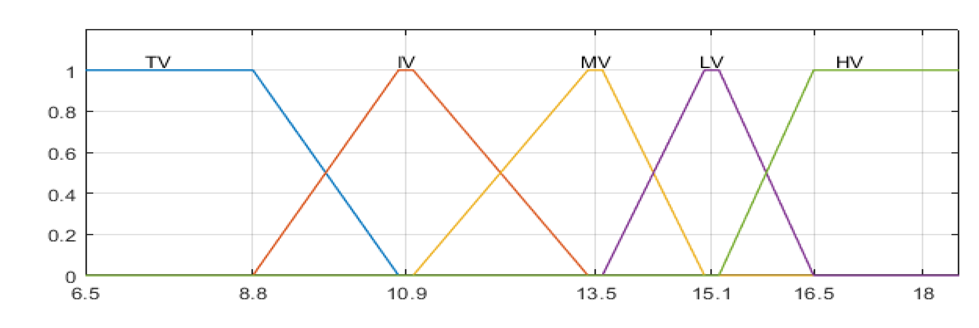
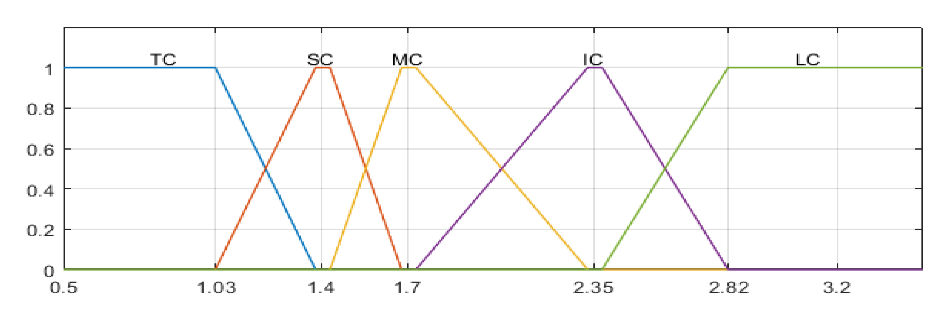
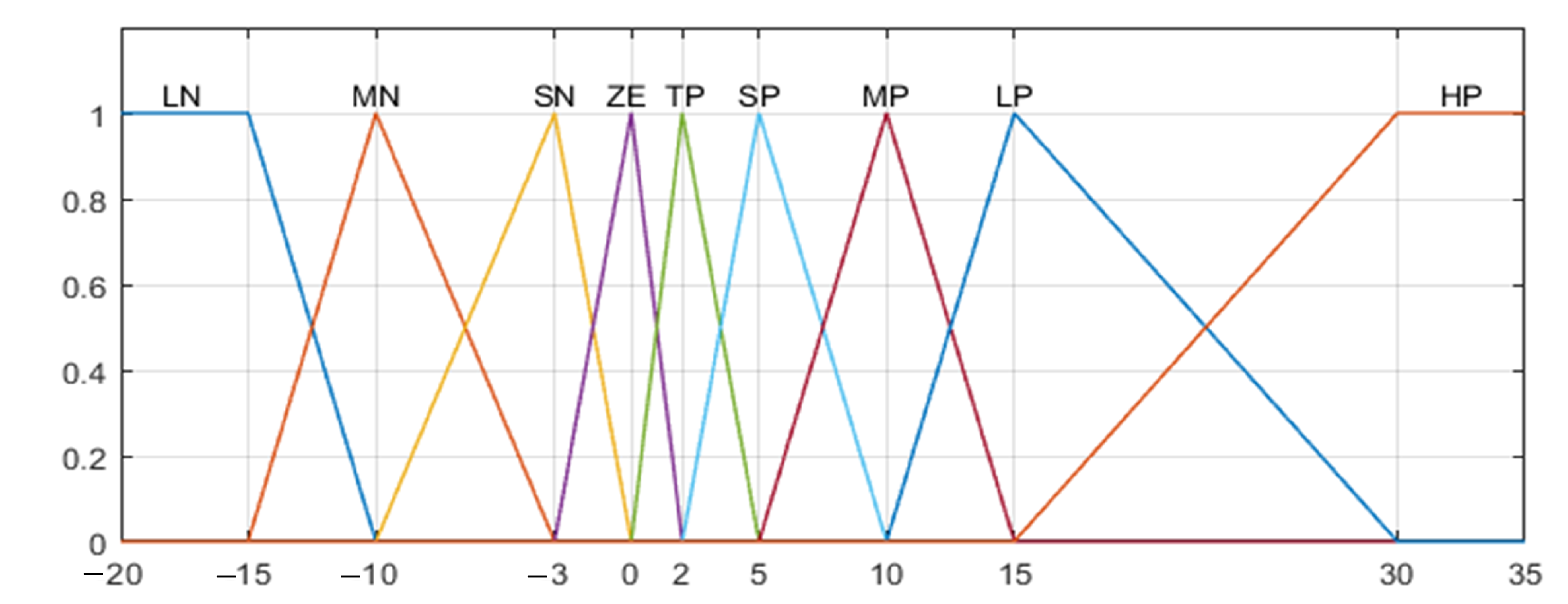
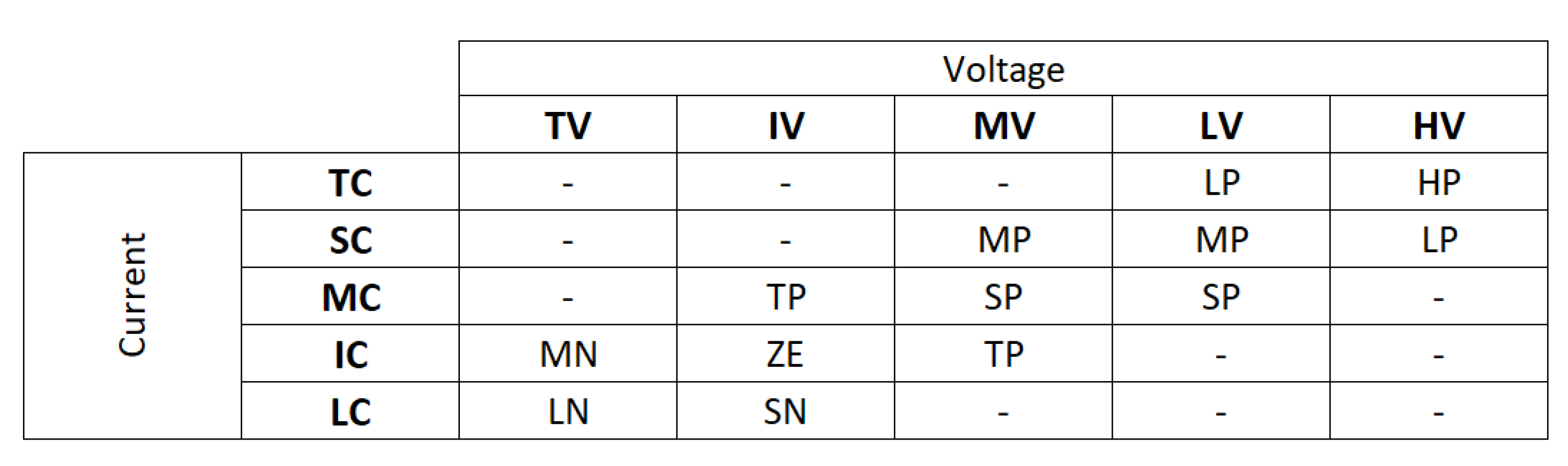
2.2. Fuzzy Logic Stage

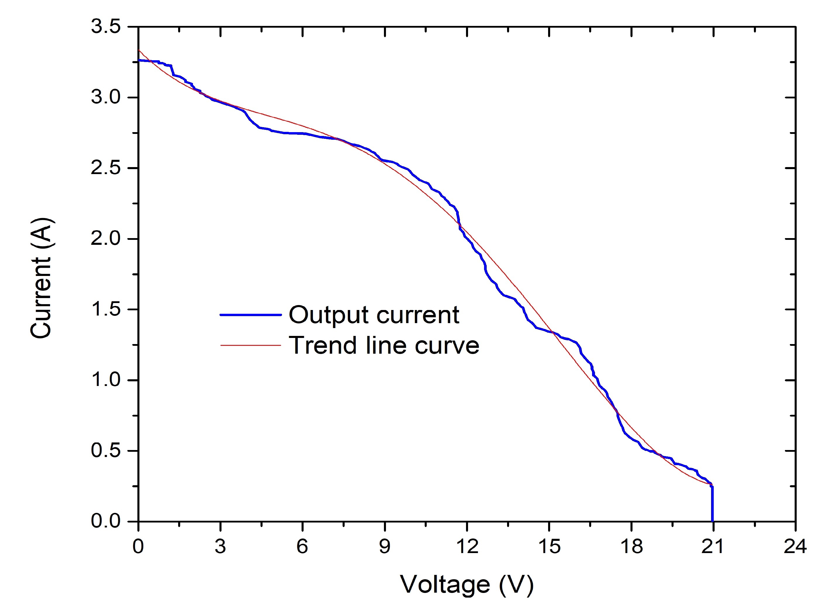
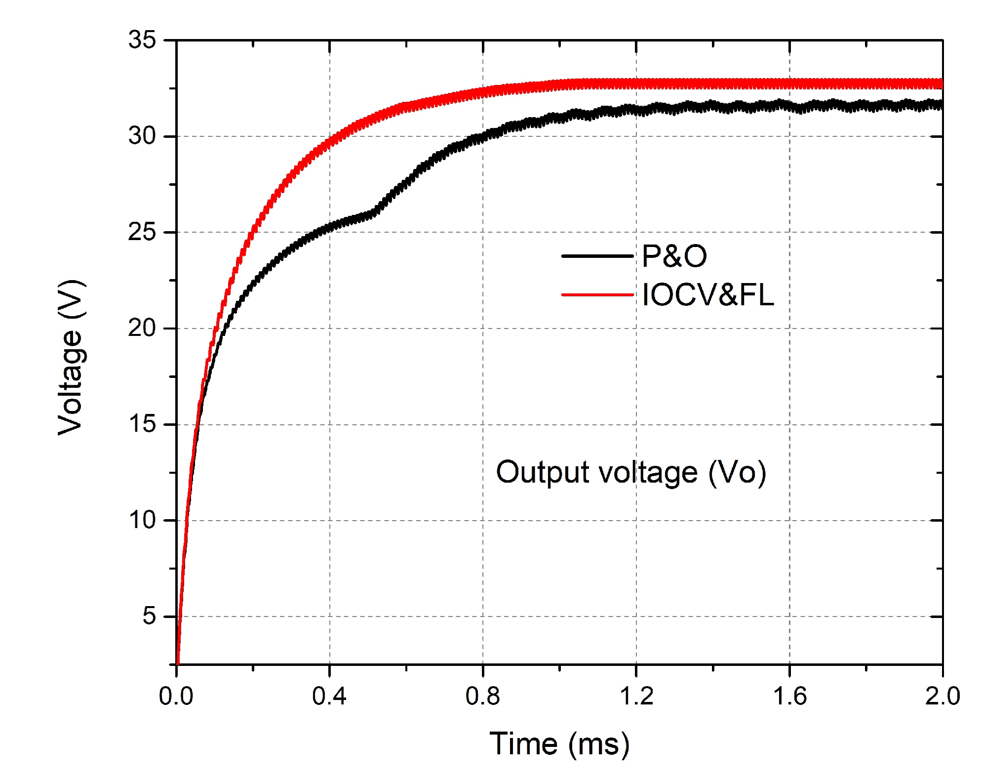
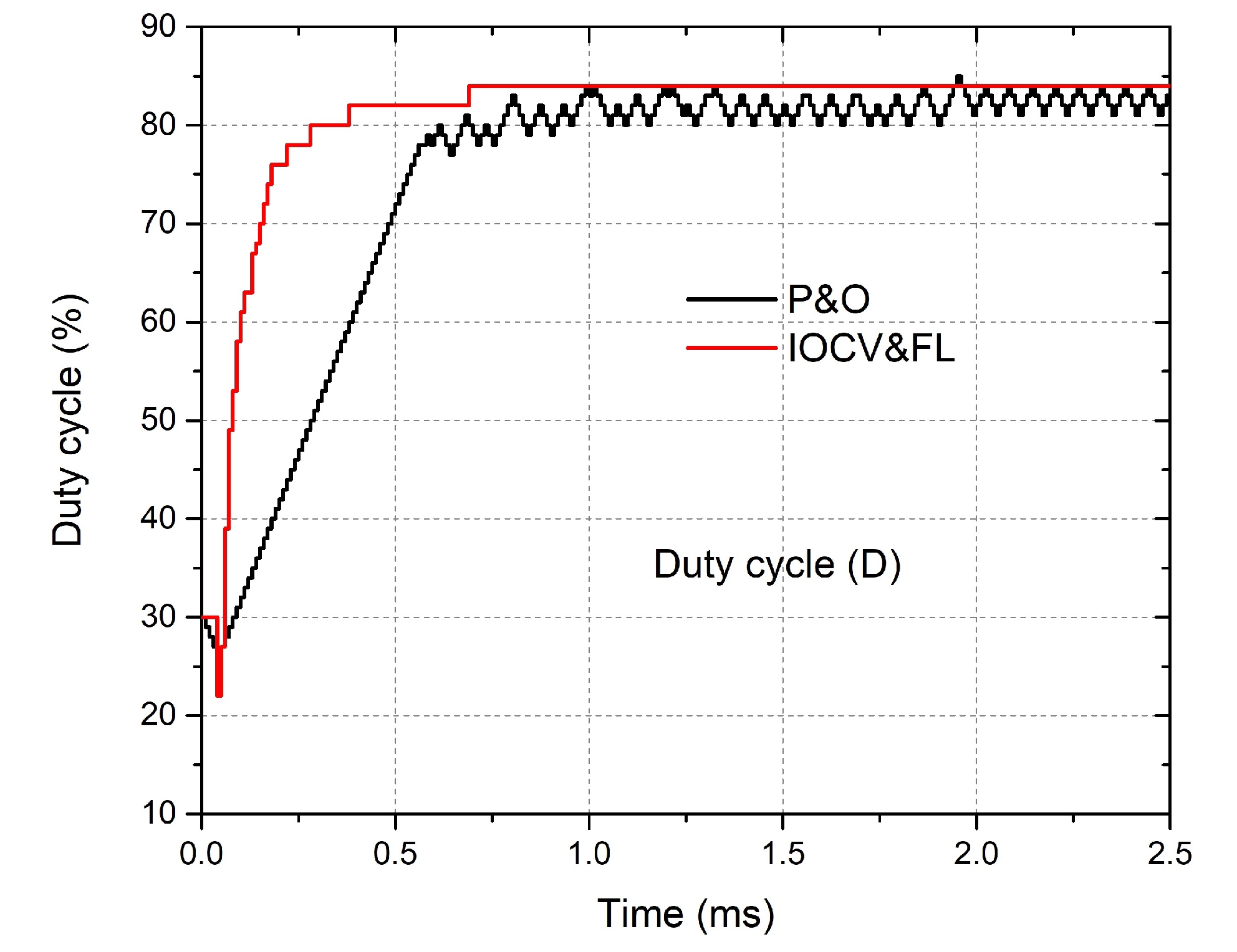
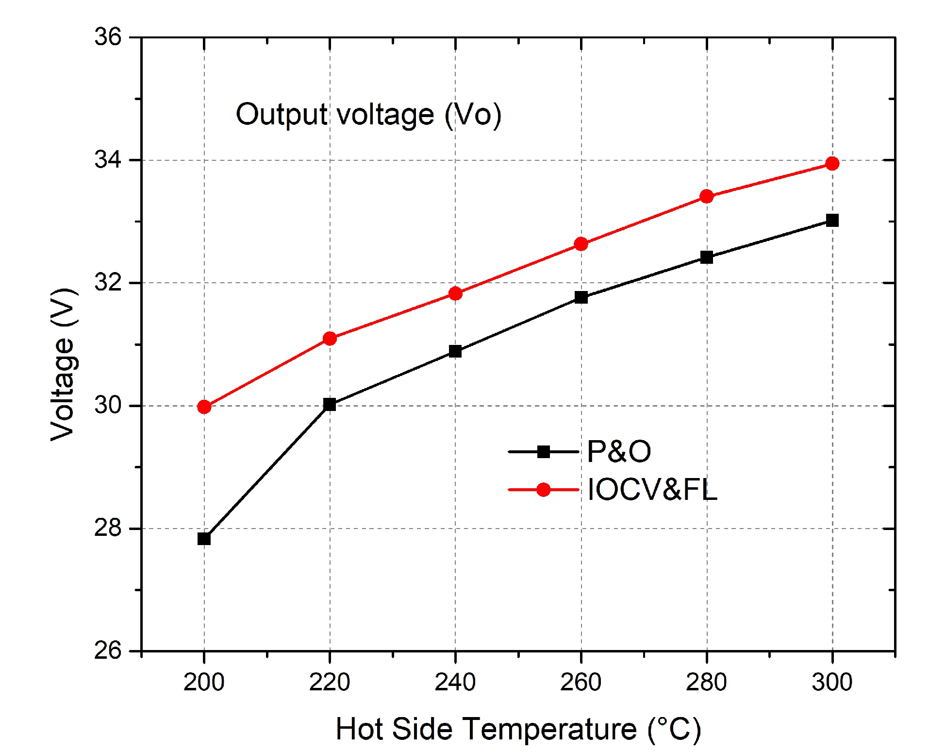
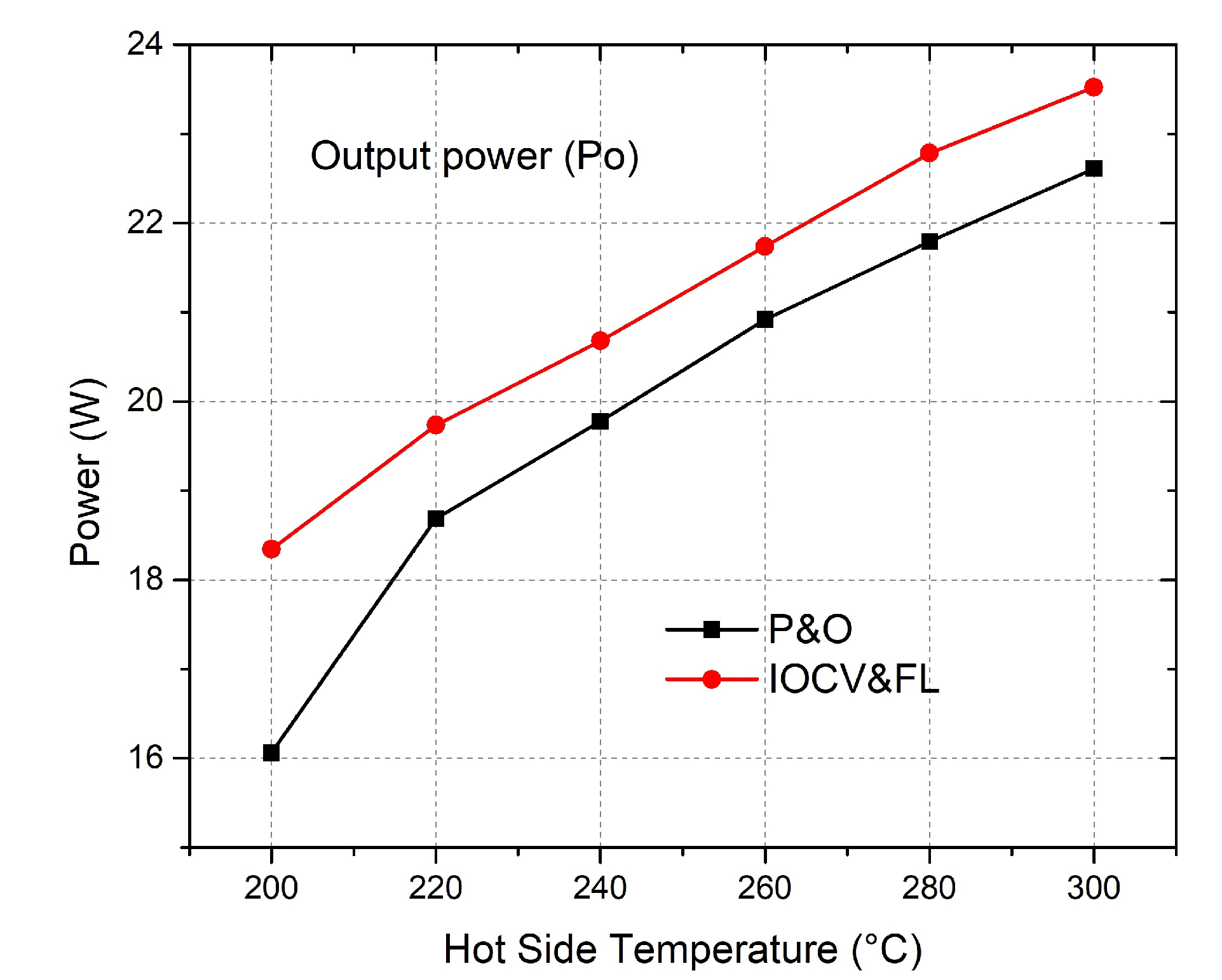
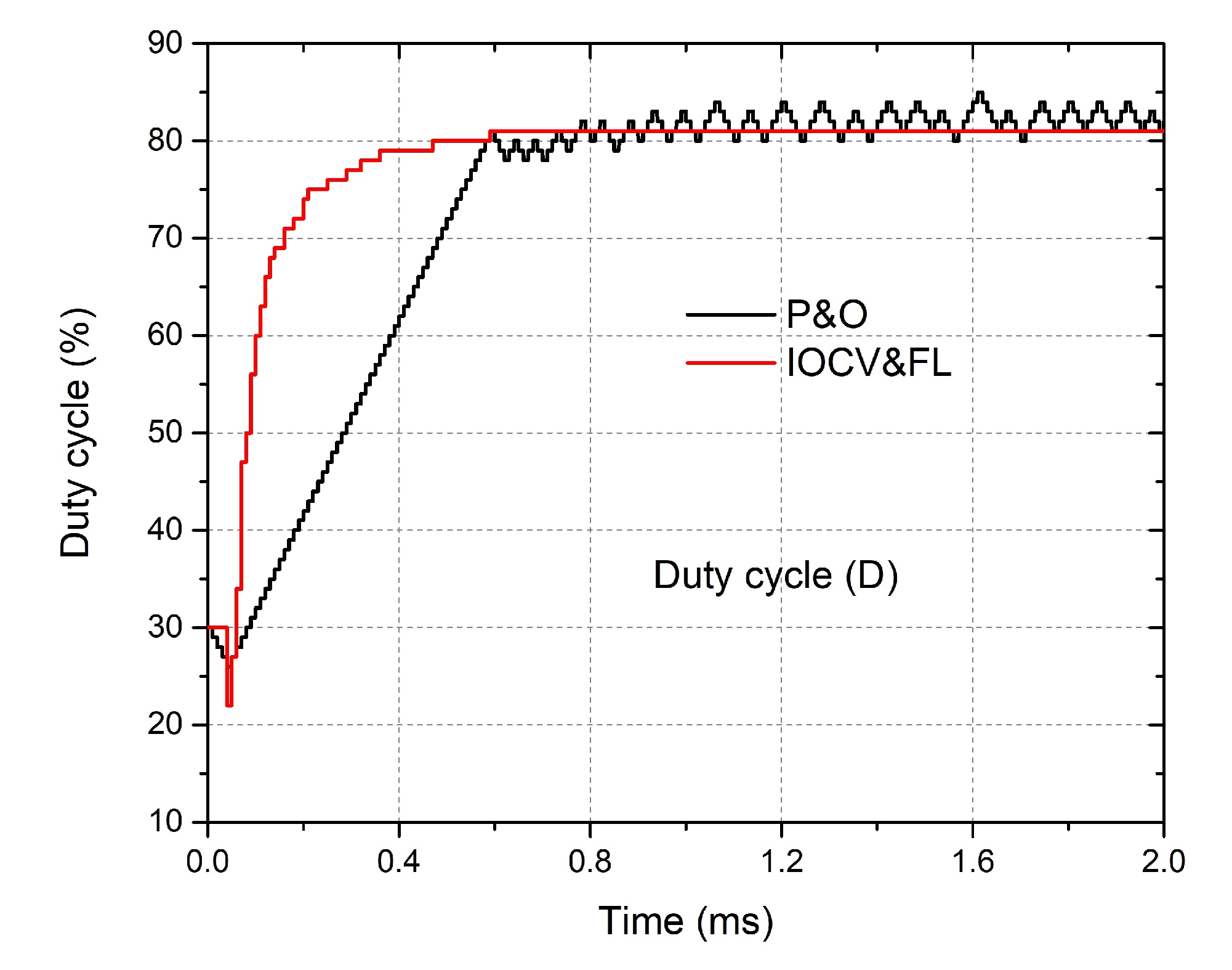
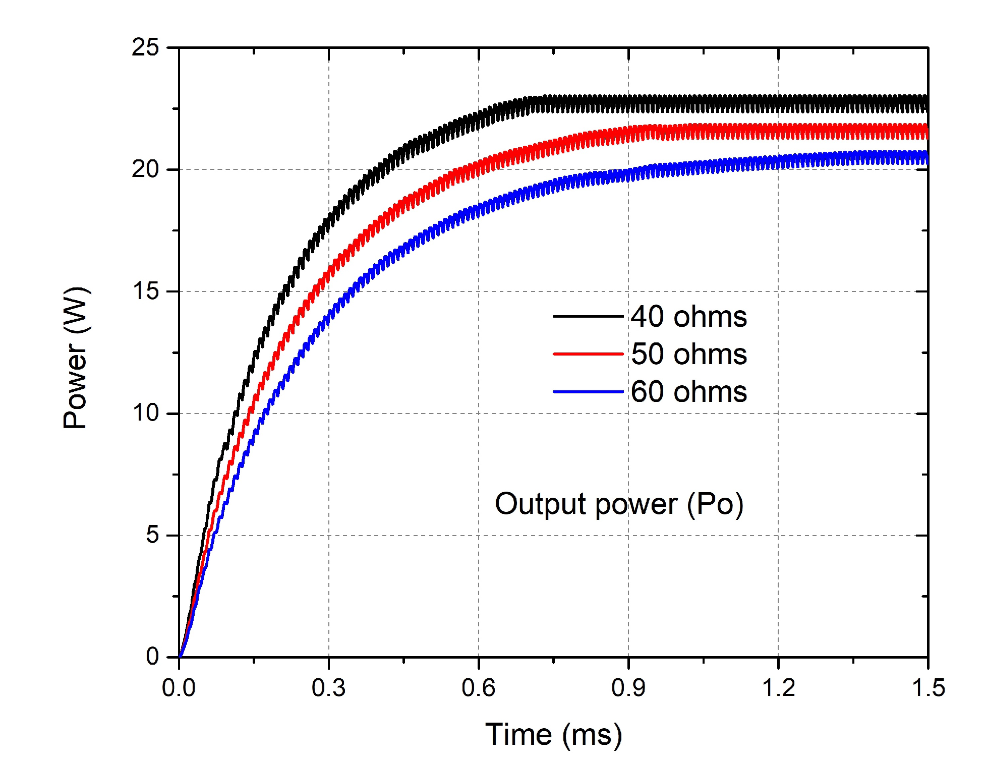
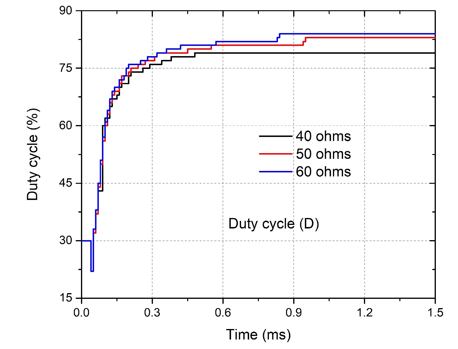
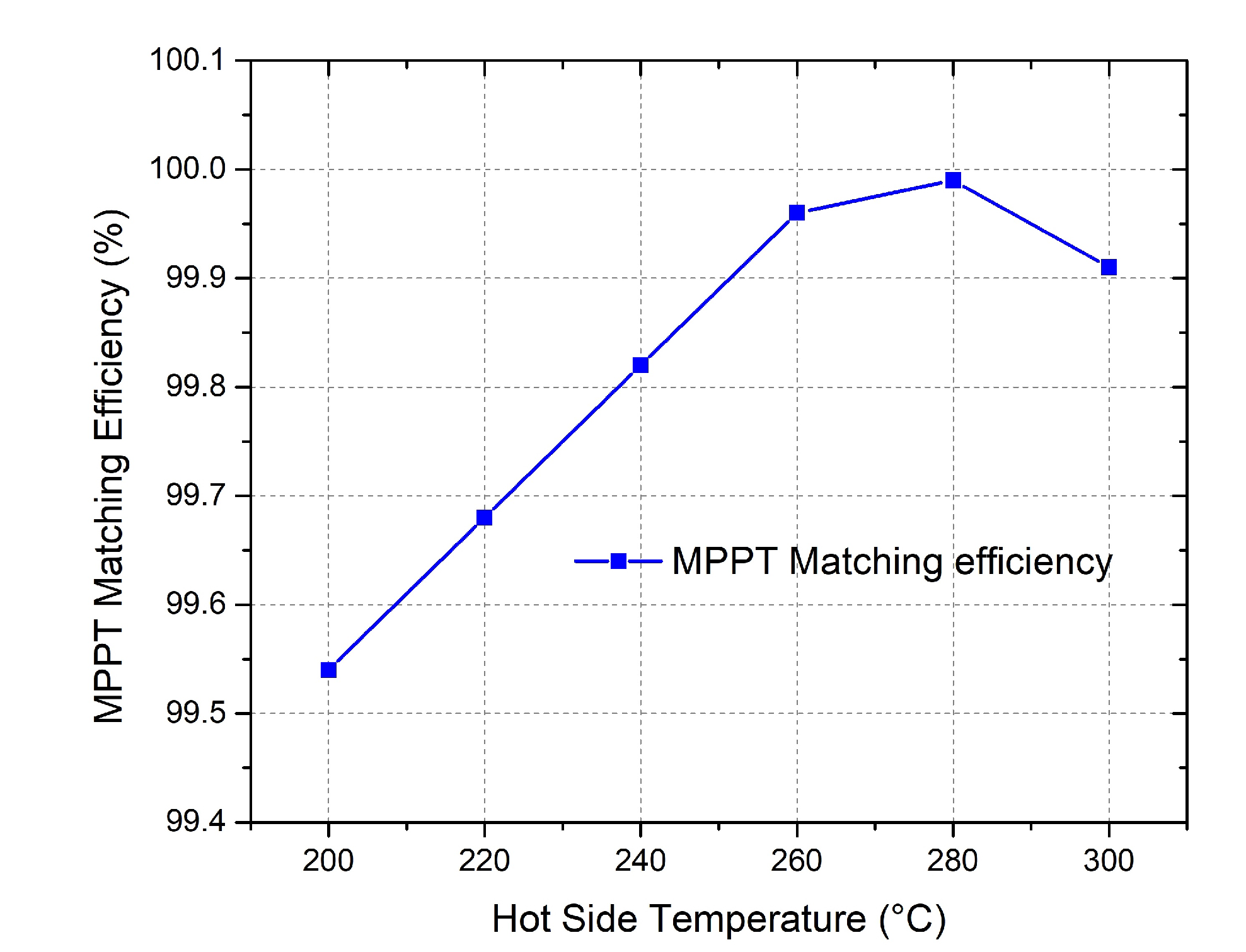
If the first stage of the algorithm does not extract the maximum power, a second stage starts to find it. This stage uses fuzzy logic and reads the input voltage and input current to recalculate the near-optimal duty cycle. At this stage, there are two inputs (voltage and current) and one output (change in duty cycle). According to the circuit parameters (quantity and characteristics of the TEGs used), the input voltage range of 6.5 V to 19 V and the input current range of 0.5 A to 3.5 A were used. Both inputs have five membership functions. These membership functions were obtained from the input voltage and input current graphs of the TEGs connected to the converter in the simulations, when there are considerable changes in the power. The range of the five membership functions were obtained heuristically to maximize the power, obtaining an optimal operation of the circuit.

In the case of voltage, its membership functions have the following linguistic labels: TV = Tiny Voltage, IV = Ideal Voltage, MV = Medium Voltage, LV = Large Voltage and HV = Huge voltage. These membership functions are shown in Figure 5. The voltage range for the input is 6.5 V to 19 V, and the membership range of each membership role is 0 to 1.

In the case of the current, its membership functions have the following linguistic labels: TC = Tiny Current, SC = Small Current, MC = Medium Current, IC = Ideal Current and LC = Large Current. These membership functions are shown in Figure 6. The current range for the input is 0.5 A to 3.5 A, and the membership range of each membership function is 0 to 1. The range of the five membership functions were obtained heuristically to maximize the power, obtaining an optimal operation of the circuit.

The output of the system is the change in duty cycle. There are nine membership functions and its range was determined heuristically to calculate the near-optimal duty cycle as fast as possible, always looking to obtain maximum power. Its membership functions have the following linguistic labels: LN = Large Negative, MN = Medium Negative, SN = Small Negative, ZE = Zero, TP = Tiny Positive, SP = Small Positive, MP = Medium Positive, LP = Large Positive and HP = Huge Positive. These membership functions are shown in Figure 7. The range of change in the duty cycle is −20% to +35%. The defuzzification method used to calculate the change in the duty cycle was the center of the area (COA) of Mamdani.

In Figure 8, the fuzzy rule base of the designed algorithm is observed. Due to the nature of the system, there are combinations between voltage and current that do not occur during the operation of the circuit since these values are inversely proportional, i.e., the higher the voltage, the less current flow the circuit will have, and vice versa. For example, there will not be a case in which there is TV and TC, which is why in the rule base there is no such condition, and some others.

This stage calculates the near-optimal duty cycle using artificial intelligence, and applies this duty cycle to the circuit. The new values of voltage and current are read. If the power obtained is the maximum, the algorithm is working at the maximum power point. But if the power obtained is not the maximum, the algorithm returns to the start and calculates the new open-circuit voltage applying the actual duty cycle.

3. Results

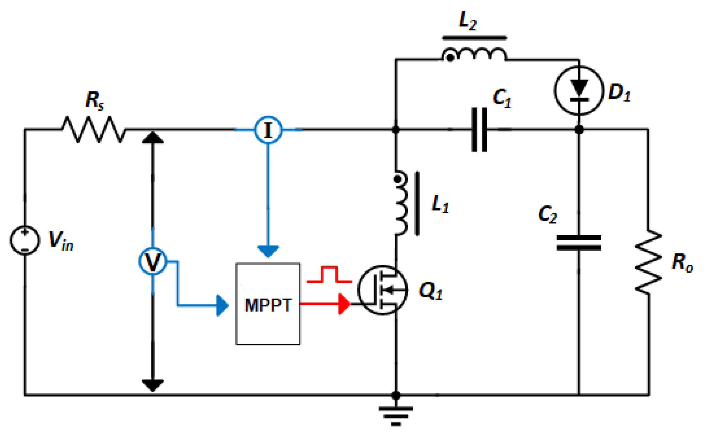
3.1. System Implementation

A simple model of the TEG is selected to be simulated and verify the concept of the proposed MPPT algorithm. The TEG model has an open-circuit voltage ($V_{in}$) of 21.3 V and internal resistance ($R_s$) of 4.4 $\Omega$. The initial parameters are a switching frequency of 100 kHz, a minimum duty cycle of 10%, a maximum duty cycle of 90%, an initial duty cycle of 30%, a simulation time of 2 ms, the time step of $1\times {10}^{-7}$ s. For the load, a resistive load of 48.22 $\Omega$ ($R_o$) of 19.29 W ($P_o$) was selected, supplied with a voltage of 30.5 V ($V_o$). The inductor $L_1$ has a value of 64.62 $\mathsf{\mu }$H, $L_2$ has a value of 6.65 $\mathsf{\mu }$H, capacitors $C_1$ and $C_2$ have a value of 10 $\mathsf{\mu }$F each. These design parameters are shown in

Table 1. Design Parameters of the TEG module and converter.

Symbol	Parameter	Value
$V_{in}$	Open-circuit voltage	21.3 V
$R_s$	Internal resistance of the TEGs	4.4 $\Omega$
$R_o$	Load	48.22 $\Omega$
$V_o$	Output voltage	30.5 V
$P_o$	Output power	19.29 W
$L_1$	Primary inductor	64.62 $\mathsf{\mu }$H
$R_{L_1}$	Parasitic resistance of $L_1$	915 m$\Omega$
$L_2$	Secondary inductor	6.65 $\mathsf{\mu }$H
$R_{L_2}$	Parasitic resistance of $L_2$	143 m$\Omega$
K	Transformer coupling	0.9
M	Mosfet model IRF540N
$R_{ds\left(ON\right)}$	Drain source resistor	50 m$\Omega$
D	Diode model 1N4934
$C_1$	Input capacitor	10 $\mathsf{\mu }$F
$C_2$	Output capacitor	10 $\mathsf{\mu }$F
$f_s$	Switching frequency	100 kHz

.

The schematic diagram of the design energy harvester is shown in Figure 9. This converter has as source a TEG with its internal resistance, only one switch (one MOSFET), one transformer without galvanic isolation, two capacitors, and the load. The MPPT controller applied an initial duty cycle, and then takes the input voltage and input current from the converter, using these values to calculate the near-optimal duty cycle using the indirect measurement of open-circuit voltage or using fuzzy logic. The blue lines indicate the input signals to the algorithm in Python and the red line is the PWM signal that goes to the converter.

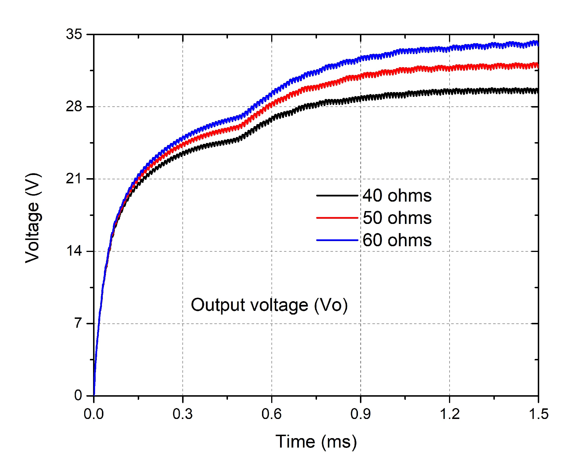
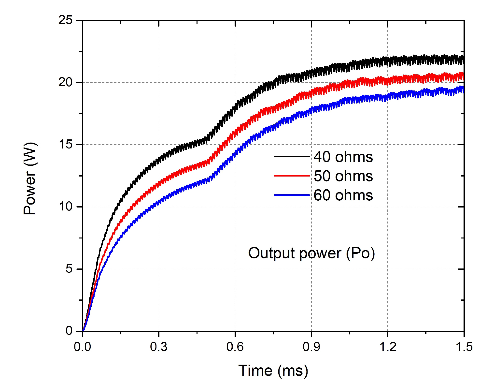
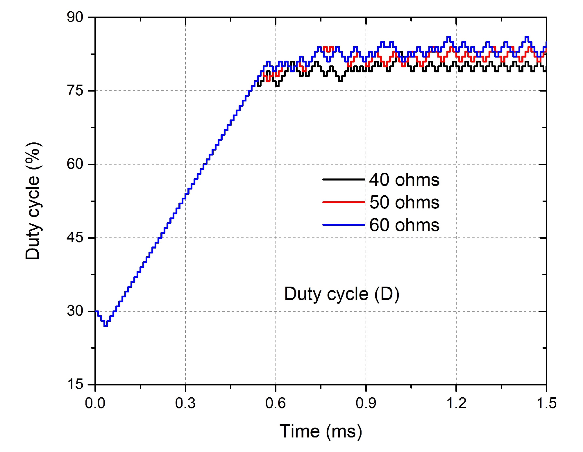
3.2. Simulation Results

To simulate the proposed MPPT algorithm (IOCV&FL), the flyback variant converter is implemented in PSIM software. The chosen maximum power point-tracking technique to compare with the IOCV&FL technique was Perturb and Observe (P&O). The results of this comparison are explained and shown in this section.

The output voltage obtained with a fixed input of 21.3 $V_{oc}$ is shown in Figure 10. The average output voltage using P&O algorithm is 31.65 V, the output current is 656.49 mA, the output power is 20.78 W, the input power is 24.24 W, and the efficiency is 85.72%. The values obtained using the proposed algorithm are an output voltage of 32.81 V, an output current of 669.90 mA, an output power of 21.98 W, an input power of 24.18 W, and an efficiency of 90.9%. The output power obtained is shown in Figure 11.

The power obtained by the proposed algorithm in the transitory state is larger than that using the P&O algorithm and, in steady state, the power is 5.77% larger than the power obtained using P&O algorithm. The duty cycle obtained using the proposed algorithm is 81% and using P&O is from 81% to 84% (see Figure 12).

With a hot-side temperature of 200 ${}^{\circ }$C, the open-circuit voltage ($V_{oc}$) is 19.8 V. When the temperature is 220 ${}^{\circ }$C, the $V_{oc}$ is 20.3 V. With a temperature of 240 ${}^{\circ }$C, the $V_{oc}$ is 20.8 V. When the temperature is 260 ${}^{\circ }$C, the $V_{oc}$ is 21.3 V. With a temperature of 280 ${}^{\circ }$C, the $V_{oc}$ is 21.8 V, and when the temperature is 300 ${}^{\circ }$C, the $V_{oc}$ is 22.3 V. These values are the input of the DC–DC converter, and the values of the output voltage obtained with these hot-side temperatures are shown in Figure 13.

The power obtained by the proposed algorithm has a range of 3.9% to 5.6% larger than the power obtained using P&O algorithm. The values are shown in Figure 14.

When the input voltage ($V_{oc}$) starts in 19.8 V and at 0.8 ms increases to 20.3 V, at 1 ms increases to 20.8 V, at 1.2 ms increases to 21.3 V, at 1.4 ms increases to 21.8 V and at 1.6 ms increases to 22.3 V. These changes generate a change in the duty cycle of the converter. The final duty cycle obtained using the proposed algorithm is 84% and using P&O algorithm is from 81% to 84% (see Figure 15).

The summary of the results obtained in the simulation is shown in

Table 2. Results obtained from simulation.

Case	Technique	Parameter	Value
1	P&O	$P_o$	20.78 W
1	IOCV&FL	$P_o$	21.98 W
2	P&O	$P_o$	21.77 W
2	IOCV&FL	$P_o$	22.72 W
3	P&O	$P_o$	18.84 W
3	IOCV&FL	$P_o$	19.80 W

. There are three different cases. Case 1 is when the input voltage ($V_{oc}$) is fixed with a value of 21.3 V, the output power ($P_o$) obtained using the proposed algorithm is 21.98 W and the efficiency ($\eta$) obtained is 90.9%. The output power obtained using the P&O algorithm is 20.78 W and its efficiency is 85.72%.

Case 2 is when the ($V_{oc}$) starts with a value of 19.8 V and at 0.8 ms increases to 20.3 V, at 1 ms increases to 20.8 V, at 1.2 ms increases to 21.3 V, at 1.4 ms increases to 21.8 and at 1.6 ms increases to 22.3 V, the values obtained using the proposed algorithm are an output power of 22.72 W and 79.94% of efficiency, an output power of 21.77 W and 82.83% of efficiency are obtained using the P&O algorithm.

Case 3 is when the ($V_{oc}$) starts with a value of 22.3 V and at 0.8 ms decreases to 21.8 V, at 1 ms decreases to 21.3 V, at 1.2 ms decreases to 20.8 V, at 1.4 ms decreases to 20.3 V and at 1.6 ms decreases to 19.8 V, the output power obtained using the proposed algorithm is 19.8 W and the efficiency obtained is 87.61%, the output power obtained using the P&O algorithm is 18.84 W and its efficiency is 88.95%.

Figure 16 shows the output voltage obtained from different values of the load (40, 50 y 60 $\Omega$) when the P&O algorithm is used. The average output voltage obtained using 40 $\Omega$ is 29.6 V, 32.03 V using 50 $\Omega$ and 34.11 V using 60 $\Omega$. The output power obtained using the P&O algorithm is shown in Figure 17. The average output power obtained for a load of 40 $\Omega$ is 21.9 W, 20.52 W for 50 $\Omega$ and 19.4 W for 60 $\Omega$. The duty cycle obtained for these different values of the load is shown in Figure 18.

Figure 19 shows the output voltage obtained from different values of the load (40, 50 y 60 $\Omega$) when the proposed algorithm is used. The average output voltage obtained using 40 $\Omega$ is 30.88 V, 33.69 V using 50 $\Omega$ and 36 V using 60 $\Omega$.

The output power obtained using the proposed algorithm is shown in Figure 20. The average output power obtained for a load of 40 $\Omega$ is 22.79 W, 21.65 W for 50 $\Omega$ and 20.57 W for 60 $\Omega$. The duty cycle obtained for these different values of the load is shown in Figure 21, the final duty cycle is 79% for a load of 40 $\Omega$, 83% for a load of 50 $\Omega$ and 84% for a load of 60 $\Omega$. With the values obtained from the simulation, it can be determined that the power obtained using the proposed algorithm is 4% larger than using P&O algorithm when the load is 40 $\Omega$, 5.5% larger for a load of 50 $\Omega$ and 6% larger for a load of 60 $\Omega$.

The MPPT matching efficiency reported in Figure 22 is defined by the following equation [32]:

$${\eta }_{match}=\frac{P_{in}}{P_{match}}$$

(33)

where $P_{in}$ is the actual input power of the DC–DC converter, and $P_{match}$ is the input power of the DC–DC converter when the matched-load condition is met, i.e., the maximum possible value of $P_{in}$ when the circuit is working at the maximum power point. From different power values at different temperatures, it is possible to compute the MPPT matched efficiencies. The matching efficiencies for the 200 ${}^{\circ }$C from to 300 ${}^{\circ }$C temperature range are 99.54% from to 99.99%.

4. Conclusions

The study of maximum power point control algorithms, focused on improving the efficiency of energy-harvesting systems based on thermoelectric generators, has allowed a greater use of TEGs in different applications. To efficiently capture and consume thermal energy, we propose the design of a MPPT algorithm for thermoelectric generators, using a combination of fractional open-circuit voltage and fuzzy logic techniques for indirect measurement of the open-circuit voltage, short-circuit current, voltage, and current at the maximum power point and calculates the near-optimal duty cycle $D_{MPP}$ (duty cycle at the maximum power point). In addition, we establish the relationship between the topology of the converter and the characteristics of the power source (TEGs) to find the maximum power point of the system.

The advantages of the proposed algorithm include a fast-tracking for the MPPT under dynamically changing conditions. Furthermore, it is significantly less than the time taken by the conventional P&O method. The power obtained by the proposed algorithm in the transitory state is larger than the P&O technique. Additionally, there are no steady-state oscillations, and therefore power loss is considerably reduced in the proposed method. With an initial duty cycle, it can calculate the open-circuit voltage and short-circuit current indirectly without the need to disconnect the converter of the source, using the inherent characteristics of the TEG I–V curve that is independent of operating and environmental conditions.

To verify the effectiveness of the proposed MPPT algorithm, the simulation results substantiate that the tracking time of IOCV&FL method is only two sampling periods and is independent of the changes in temperature and load conditions. We compare it with the P&O technique in different scenarios (three cases) and the results obtained indicate that the designed algorithm provides between 3.9% and 5.6% more power to the load than the P&O technique in a 20 W system. Furthermore, the power obtained in transient state is greater. The processing time of the proposed algorithm is lower, and it reaches the near-optimal duty cycle faster than using the P&O algorithm.

References

1. Champier, D.; Bédécarrats, J.P.; Kousksou, T.; Rivaletto, M.; Strub, F.; Pignolet, P. Study of a TE (thermoelectric) generator incorporated in a multifunction wood stove. Energy 2011, 36, 1518–1526. [Google Scholar] [CrossRef] [Green Version]
2. Montecucco, A.; Knox, A.R. Maximum power point tracking converter based on the open-circuit voltage method for thermoelectric generators. IEEE Trans. Power Electron. 2015, 30, 828–839. [Google Scholar] [CrossRef]
3. Dalala, Z.M.; Saadeh, O.; Bdour, M.; Zahid, Z.U. A new maximum power point tracking (MPPT) algorithm for thermoelectric generators with reduced voltage sensors count control. Energies 2018, 11, 1826. [Google Scholar] [CrossRef] [Green Version]
4. Rowe, D.M. Thermoelectric waste heat recovery as a renewable energy source. Int. J. Innov. Energy Syst. Power 2006, 1, 13–23. [Google Scholar]
5. Yahya, K.; Bilgin, M.Z.; Erfidan, T. The effect of temperature variations over thermoelectric generator efficiency. In Proceedings of the International Engineering Research Symposium UMAS2017 Duzce, Düzce, Turkey, 11–13 September 2017; pp. 192–200. [Google Scholar]
6. Mobarrez, M.; Fregosi, D.; Jalali, G.; Bhattacharya, S.; Bahmani, M.A. A novel control method for preventing the PV and load fluctuations in a DC microgrid from transferring to the AC power grid. In Proceedings of the 2017 IEEE Second International Conference on DC Microgrids (ICDCM), Nuremburg, Germany, 27–29 June 2017; pp. 352–359. [Google Scholar]
7. Adly, M.; Strunz, K. Irradiance-adaptive PV module integrated converter for high efficiency and power quality in standalone and DC microgrid applications. IEEE Trans. Ind. Electron. 2017, 65, 436–446. [Google Scholar] [CrossRef]
8. Montecucco, A.; Siviter, J.; Knox, A.R. The effect of temperature mismatch on thermoelectric generators electrically connected in series and parallel. Appl. Energy 2014, 123, 47–54. [Google Scholar] [CrossRef] [Green Version]
9. Twaha, S.; Zhu, J.; Yan, Y.; Li, B.; Huang, K. Performance analysis of thermoelectric generator using dc-dc converter with incremental conductance based maximum power point tracking. Energy Sustain. Dev. 2017, 37, 86–98. [Google Scholar] [CrossRef]
10. Zhang, T. Design and optimization considerations for thermoelectric devices. Energy Convers. Manag. 2016, 112, 404–412. [Google Scholar] [CrossRef]
11. El-Genk, M.S.; Saber, H.H.; Caillat, T. Efficient segmented thermoelectric unicouples for space power applications. Energy Convers. Manag. 2003, 44, 1755–1772. [Google Scholar] [CrossRef]
12. Hsiao, Y.Y.; Chang, W.C.; Chen, S.L. A mathematic model of thermoelectric module with applications on waste heat recovery from automobile engine. Energy 2010, 35, 1447–1454. [Google Scholar] [CrossRef]
13. Liu, X.; Deng, Y.D.; Li, Z.; Su, C.Q. Performance analysis of a waste heat recovery thermoelectric generation system for automotive application. Energy Convers. Manag. 2015, 90, 121–127. [Google Scholar] [CrossRef]
14. Goudarzi, A.M.; Mazandarani, P.; Panahi, R.; Behsaz, H.; Rezania, A.; Rosendahl, L.A. Integration of thermoelectric generators and wood stove to produce heat, hot water, and electrical power. J. Electron. Mater. 2013, 42, 2127–2133. [Google Scholar] [CrossRef]
15. Kinsella, C.E.; O’Shaughnessy, S.M.; Deasy, M.J.; Duffy, M.; Robinson, A.J. Battery charging considerations in small scale electricity generation from a thermoelectric module. Appl. Energy 2014, 114, 80–90. [Google Scholar] [CrossRef]
16. Adhithya, K.; Anand, R.; Balaji, G.; Harinarayanan, J. Battery charging using thermoelectric generation module in automobiles. IJRET Int. J. Res. Eng. Technol. 2015, 4, 296–303. [Google Scholar]
17. Ebling, D.G.; Krumm, A.; Pfeiffelmann, B.; Gottschald, J.; Bruchmann, J.; Benim, A.C.; Stunz, A. Development of a system for thermoelectric heat recovery from stationary industrial processes. J. Electron. Mater. 2016, 45, 3433–3439. [Google Scholar] [CrossRef]
18. Francioso, L.; De Pascali, C.; Sglavo, V.; Grazioli, A.; Masieri, M.; Siciliano, P. Modelling, fabrication and experimental testing of an heat sink free wearable thermoelectric generator. Energy Convers. Manag. 2017, 145, 204–213. [Google Scholar] [CrossRef]
19. Ma, Q.; Fang, H.; Zhang, M. Theoretical analysis and design optimization of thermoelectric generator. Appl. Therm. Eng. 2017, 127, 758–764. [Google Scholar] [CrossRef]
20. Wang, Y.; Dai, C.; Wang, S. Theoretical analysis of a thermoelectric generator using exhaust gas of vehicles as heat source. Appl. Energy 2013, 112, 1171–1180. [Google Scholar] [CrossRef]
21. Esram, T.; Chapman, P.L. Comparison of photovoltaic array maximum power point tracking techniques. IEEE Trans. Energy Convers. 2007, 22, 439–449. [Google Scholar] [CrossRef] [Green Version]
22. Laird, I.; Lovatt, H.; Savvides, N.; Lu, D.; Agelidis, V.G. Comparative study of maximum power point tracking algorithms for thermoelectric generators. In Proceedings of the 2008 Australasian Universities Power Engineering Conference, Sydney, NSW, Australia, 14–17 December 2008; pp. 1–6. [Google Scholar]
23. Kim, R.Y.; Lai, J.S. A seamless mode transfer maximum power point tracking controller for thermoelectric generator applications. In Proceedings of the 2007 IEEE Industry Applications Annual Meeting, New Orleans, LA, USA, 23–27 September 2007; pp. 977–984. [Google Scholar]
24. Pilawa-Podgurski, R.C.; Pallo, N.A.; Chan, W.R.; Perreault, D.J.; Celanovic, I.L. Low-power maximum power point tracker with digital control for thermophotovoltaic generators. In Proceedings of the 2010 Twenty-Fifth Annual IEEE Applied Power Electronics Conference and Exposition (APEC), Palm Springs, CA, USA, 21–25 February 2010; pp. 961–967. [Google Scholar]
25. Bunthern, K.; Long, B.; Christophe, G.; Bruno, D.; Pascal, M. Modeling and tuning of MPPT controllers for a thermoelectric generator. In Proceedings of the 2014 First International Conference on Green Energy ICGE 2014, Sfax, Tunisia, 25–27 March 2014; pp. 220–226. [Google Scholar]
26. Kollimalla, S.K.; Mishra, M.K. A novel adaptive P&O MPPT algorithm considering sudden changes in the irradiance. IEEE Trans. Energy Convers. 2014, 29, 602–610. [Google Scholar]
27. Pandey, A.; Dasgupta, N.; Mukerjee, A.K. High-performance algorithms for drift avoidance and fast tracking in solar MPPT system. IEEE Trans. Energy Convers. 2008, 23, 681–689. [Google Scholar] [CrossRef] [Green Version]
28. Montecucco, A.; Siviter, J.; Knox, A.R. Simple, fast and accurate maximum power point tracking converter for thermoelectric generators. In Proceedings of the 2012 IEEE Energy Conversion Congress and Exposition (ECCE), Raleigh, NC, USA, 15–20 September 2012; pp. 2777–2783. [Google Scholar]
29. Wu, S.J.; Wang, S.; Yang, C.J.; Xie, K.R. Energy management for thermoelectric generators based on maximum power point and load power tracking. Energy Convers. Manag. 2018, 177, 55–63. [Google Scholar] [CrossRef]
30. Marroquín-Arreola, R.; Salazar-Pérez, D.; Ponce-Silva, M.; Hernández-De León, H.; Aqui-Tapia, J.A.; Lezama, J.; Saavedra-Benítez, Y.I.; Escobar-Gómez, E.N.; Lozoya-Ponce, R.E.; Mota-Grajales, R. Analysis of a DC-DC Flyback Converter Variant for Thermoelectric Generators with Partial Energy Processing. Electronics 2021, 10, 619. [Google Scholar] [CrossRef]
31. Laird, I.; Lu, D. Steady state reliability of maximum power point tracking algorithms used with a thermoelectric generator. In Proceedings of the IEEE international symposium on circuits and systems (ISCAS), Beijing, China, 19–23 May 2013; pp. 1316–1319. [Google Scholar]
32. Li, M.; Xu, S.; Chen, Q.; Zheng, L.R. Thermoelectric generator based dc-dc conversion networks for automotive applications. J. Electron. Mater. 2011, 40, 1136–1143. [Google Scholar] [CrossRef]
Figure 1. Designed MPPT algorithm flow chart.
Energies 15 03833 g001
Figure 2. Converter used for analysis.
Energies 15 03833 g002
Figure 3. Equivalent resistance seen by the TEG.
Energies 15 03833 g003
Figure 4. The trend line of the V–I curve of the TEGs.
Energies 15 03833 g004
Figure 5. Input voltage membership functions.
Energies 15 03833 g005
Figure 6. Input current membership functions.
Energies 15 03833 g006
Figure 7. Membership functions of the change in duty cycle Δ D .
Energies 15 03833 g007
Figure 8. Fuzzy rule base of the proposed algorithm.
Energies 15 03833 g008
Figure 9. Schematic diagram of the converter used to evaluate the proposed MPPT algorithm.
Energies 15 03833 g009
Figure 10. Output voltage plot.
Energies 15 03833 g010
Figure 11. Output power plot.
Energies 15 03833 g011
Figure 12. Duty cycle plot.
Energies 15 03833 g012
Figure 13. Output voltage plot at different hot-side temperatures.
Energies 15 03833 g013
Figure 14. Output power plot at different hot-side temperatures.
Energies 15 03833 g014
Figure 15. Duty cycle plot obtained.
Energies 15 03833 g015
Figure 16. Output voltage plot obtained using P&O algorithm.
Energies 15 03833 g016
Figure 17. Output power plot obtained using P&O algorithm.
Energies 15 03833 g017
Figure 18. Duty cycle plot obtained using P&O algorithm.
Energies 15 03833 g018
Figure 19. Output voltage plot obtained using the proposed algorithm.
Energies 15 03833 g019
Figure 20. Output power plot using the proposed algorithm.
Energies 15 03833 g020
Figure 21. Duty cycle plot using the proposed algorithm.
Energies 15 03833 g021
Figure 22. MPPT matching efficiency at different hot-side temperatures for the proposed algorithm.
Energies 15 03833 g022