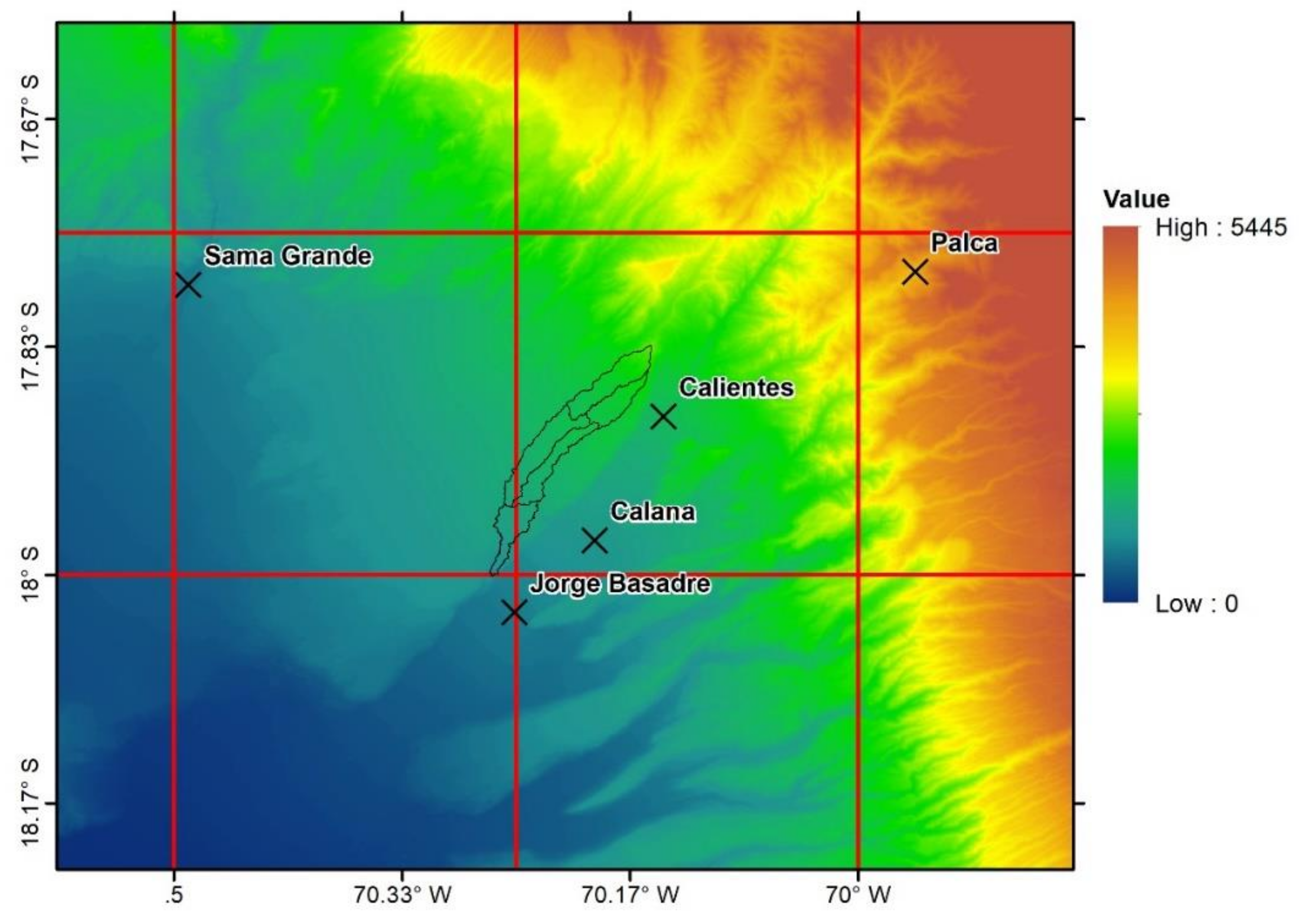
Figure 1.
Location of the Devil’s Creek with the meteorological rain gauges selected for the downscaling and cells of the general circulation models (GCMs).
Figure 1.
Location of the Devil’s Creek with the meteorological rain gauges selected for the downscaling and cells of the general circulation models (GCMs).
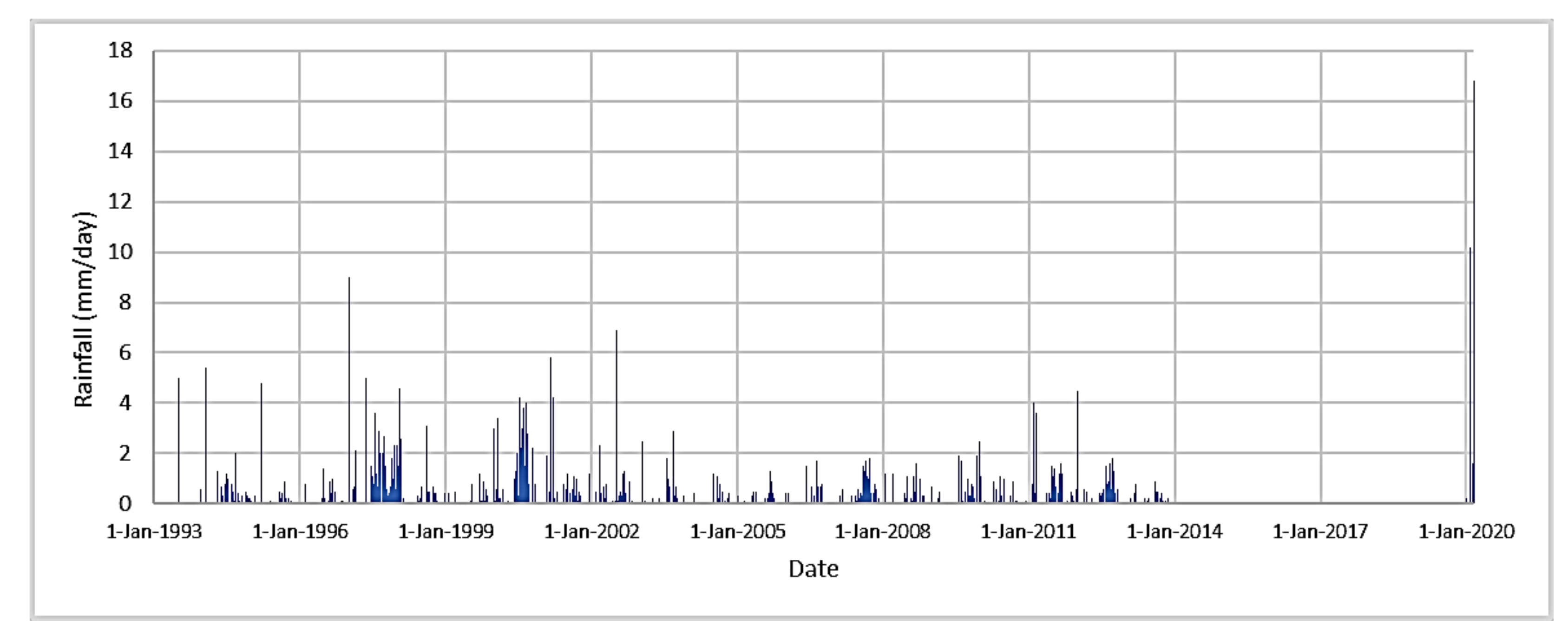
Figure 2.
Total daily precipitation—JORGE BASADRE rain gauge.
Figure 2.
Total daily precipitation—JORGE BASADRE rain gauge.
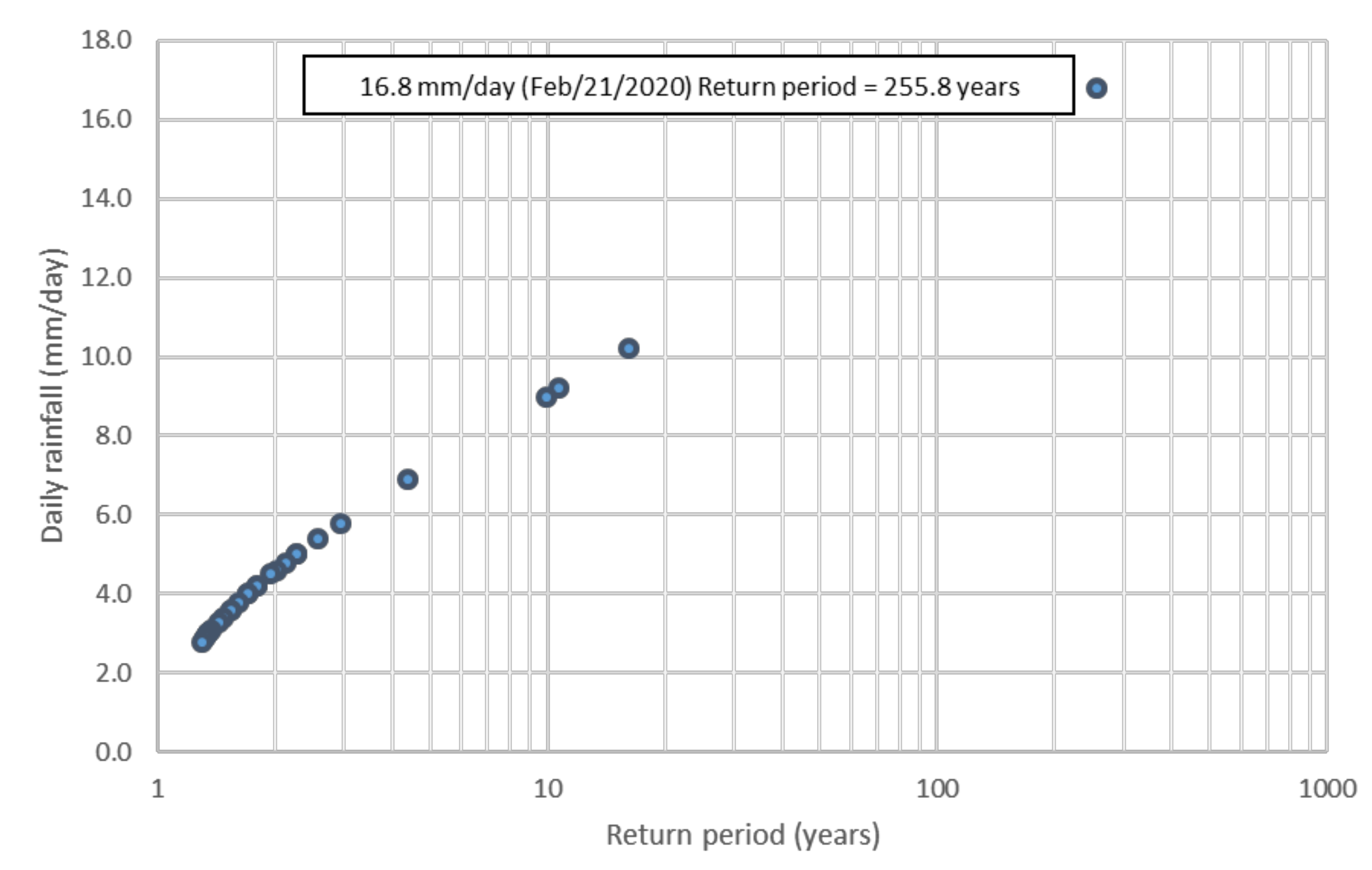
Figure 3.
Frequency analysis of the partial series of total daily precipitation at JORGE BASADRE rain gauge (from 1993 to 2020).
Figure 3.
Frequency analysis of the partial series of total daily precipitation at JORGE BASADRE rain gauge (from 1993 to 2020).
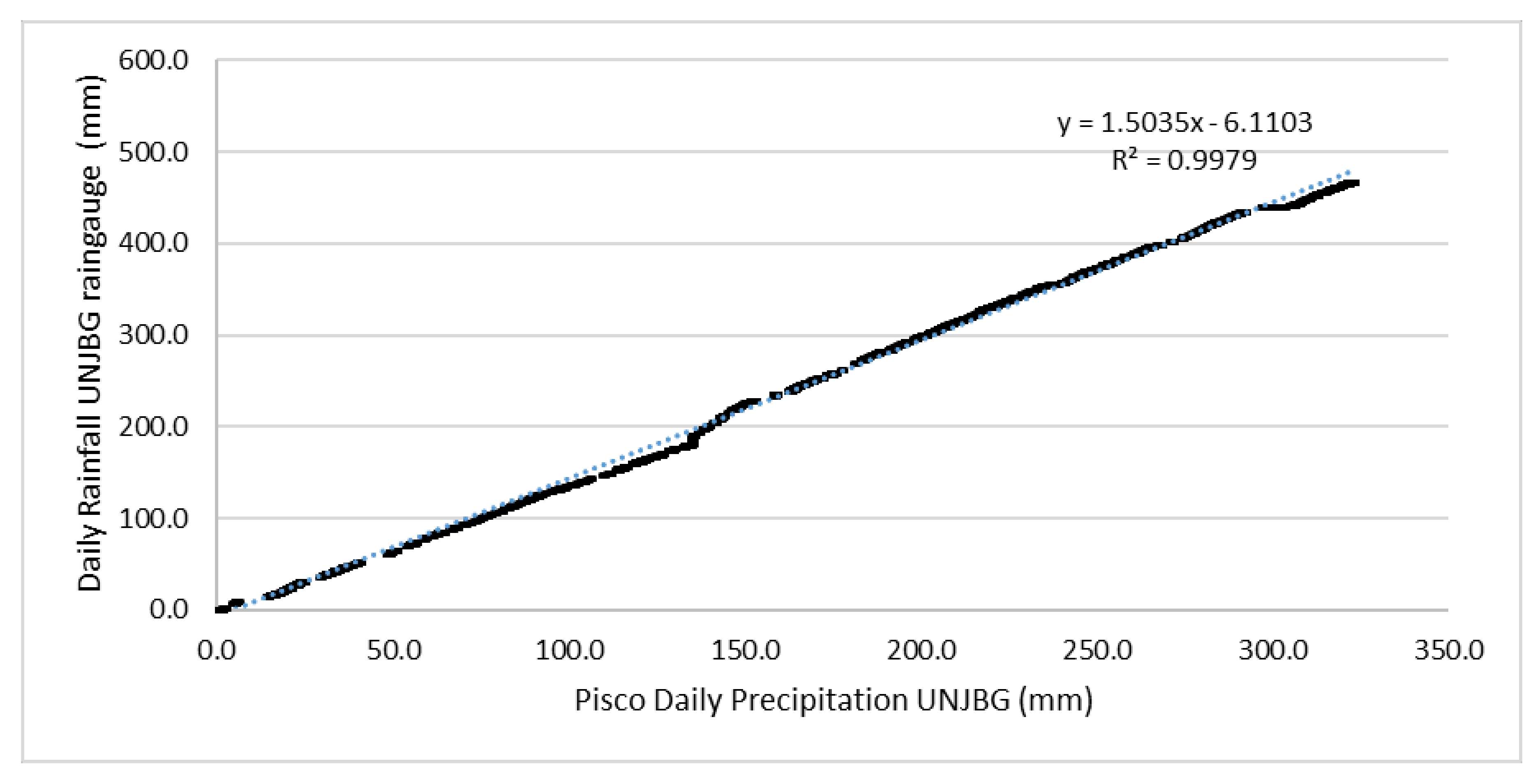
Figure 4.
Comparison double-mass between the precipitation data of the PISCO product in JORGE BASADRE rain gauge and the rainfall of the JORGE BASADRE rain gauge, during 7780 days (1 January 1993–21 April 2014).
Figure 4.
Comparison double-mass between the precipitation data of the PISCO product in JORGE BASADRE rain gauge and the rainfall of the JORGE BASADRE rain gauge, during 7780 days (1 January 1993–21 April 2014).
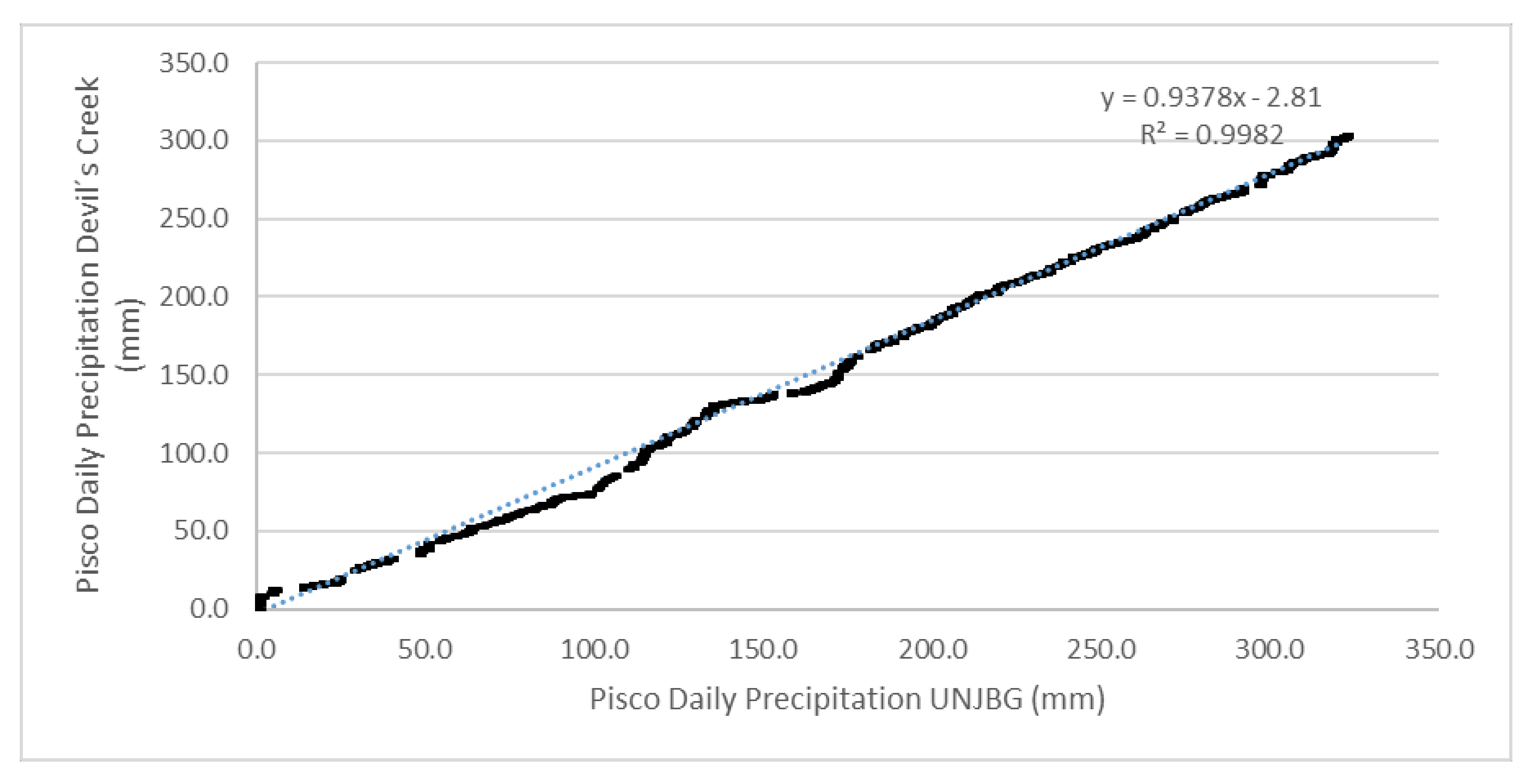
Figure 5.
Comparation double-mass between the precipitation data of the PISCO product in the JORGE BASADRE rain gauge versus the precipitation data of the PISCO product in Devil’s Creek over 7780 days (1 January 1993–21 April 2014).
Figure 5.
Comparation double-mass between the precipitation data of the PISCO product in the JORGE BASADRE rain gauge versus the precipitation data of the PISCO product in Devil’s Creek over 7780 days (1 January 1993–21 April 2014).
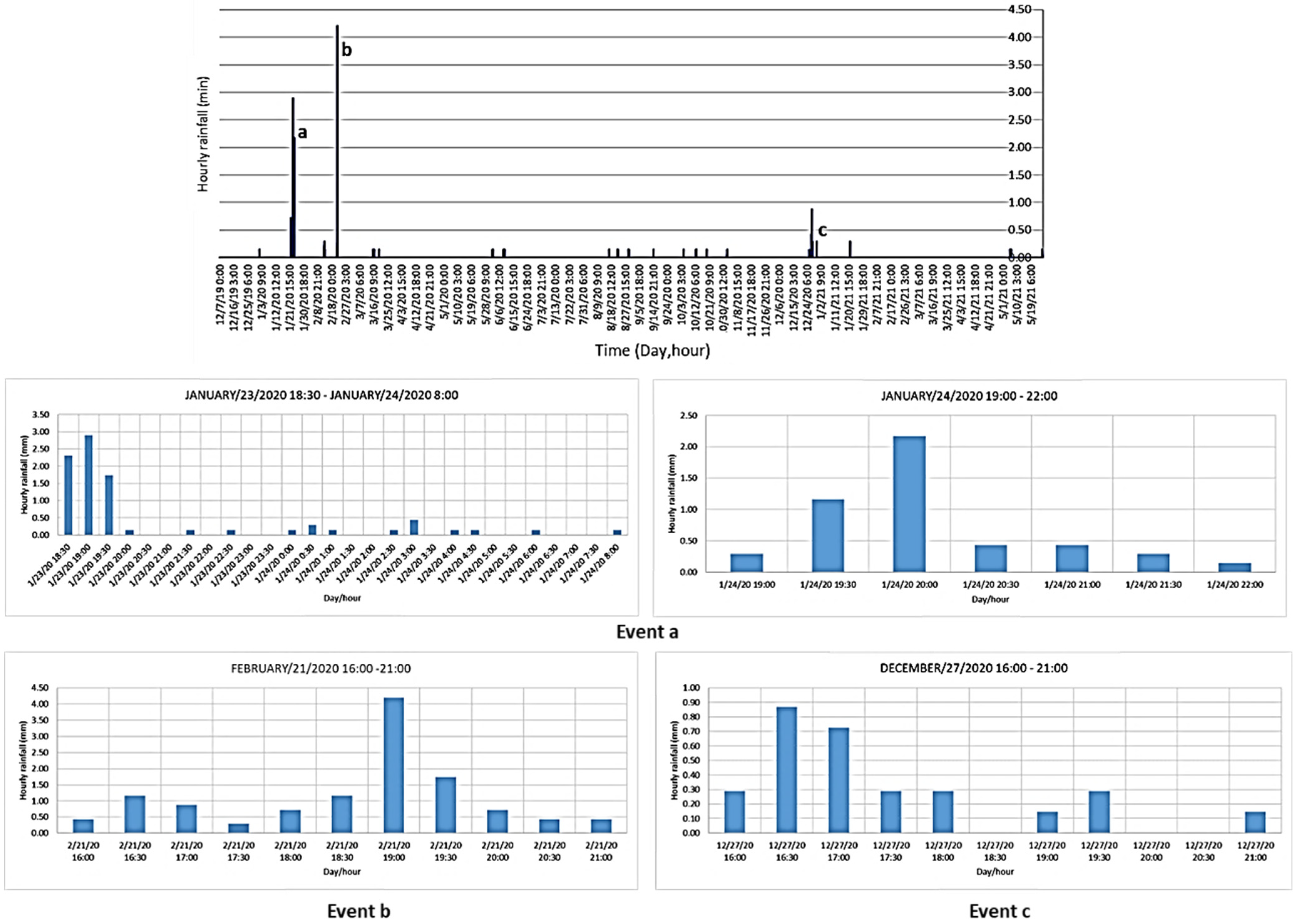
Figure 6.
Estimated hourly rainfall for the Devil’s Creek. (a) Event on 23–24 January 2020; (b) event on 21 February 2020; and (c) event on 27 December 2020.
Figure 6.
Estimated hourly rainfall for the Devil’s Creek. (a) Event on 23–24 January 2020; (b) event on 21 February 2020; and (c) event on 27 December 2020.
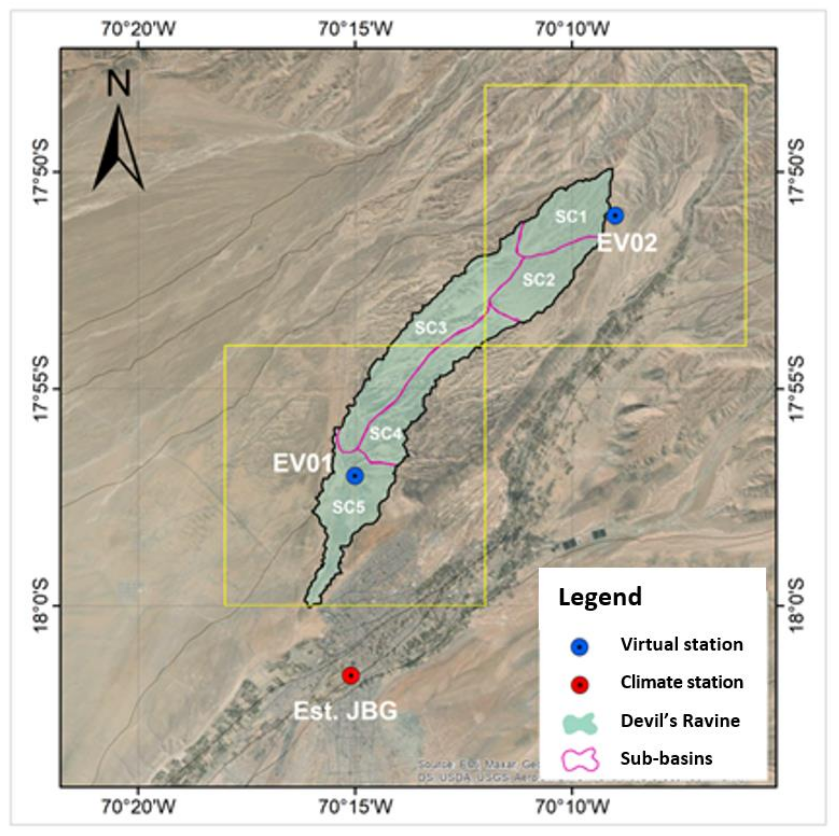
Figure 7.
Location of virtual rain gauges and the JORGE BASADRE rain gauge.
Figure 7.
Location of virtual rain gauges and the JORGE BASADRE rain gauge.
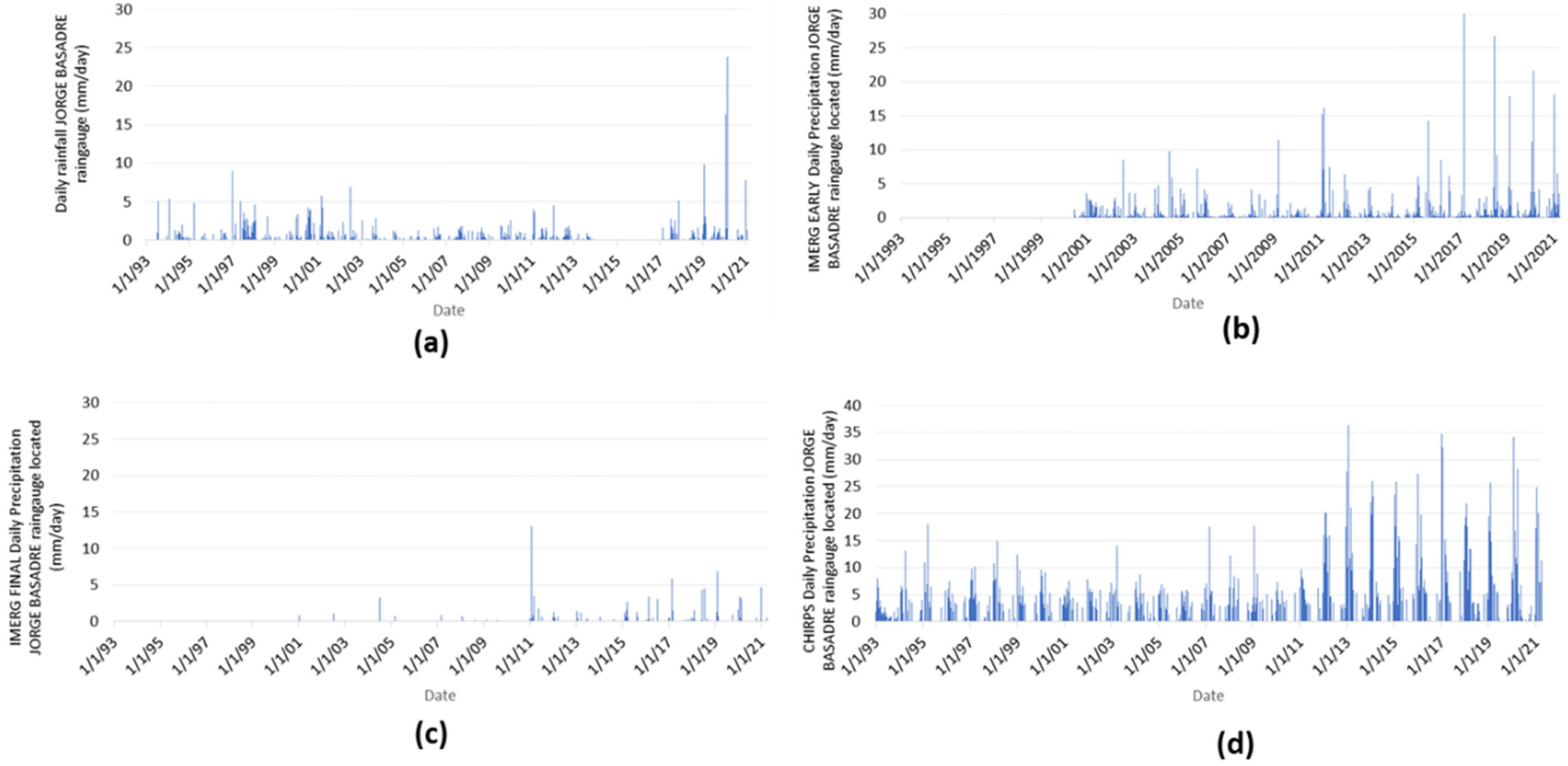
Figure 8.
Comparation between (a) daily rainfall in JORGE BASADRE rain gauge and daily precipitation from satellites products: (b) IMERG Early, (c) IMERG Final, and (d) CHIRPS.
Figure 8.
Comparation between (a) daily rainfall in JORGE BASADRE rain gauge and daily precipitation from satellites products: (b) IMERG Early, (c) IMERG Final, and (d) CHIRPS.
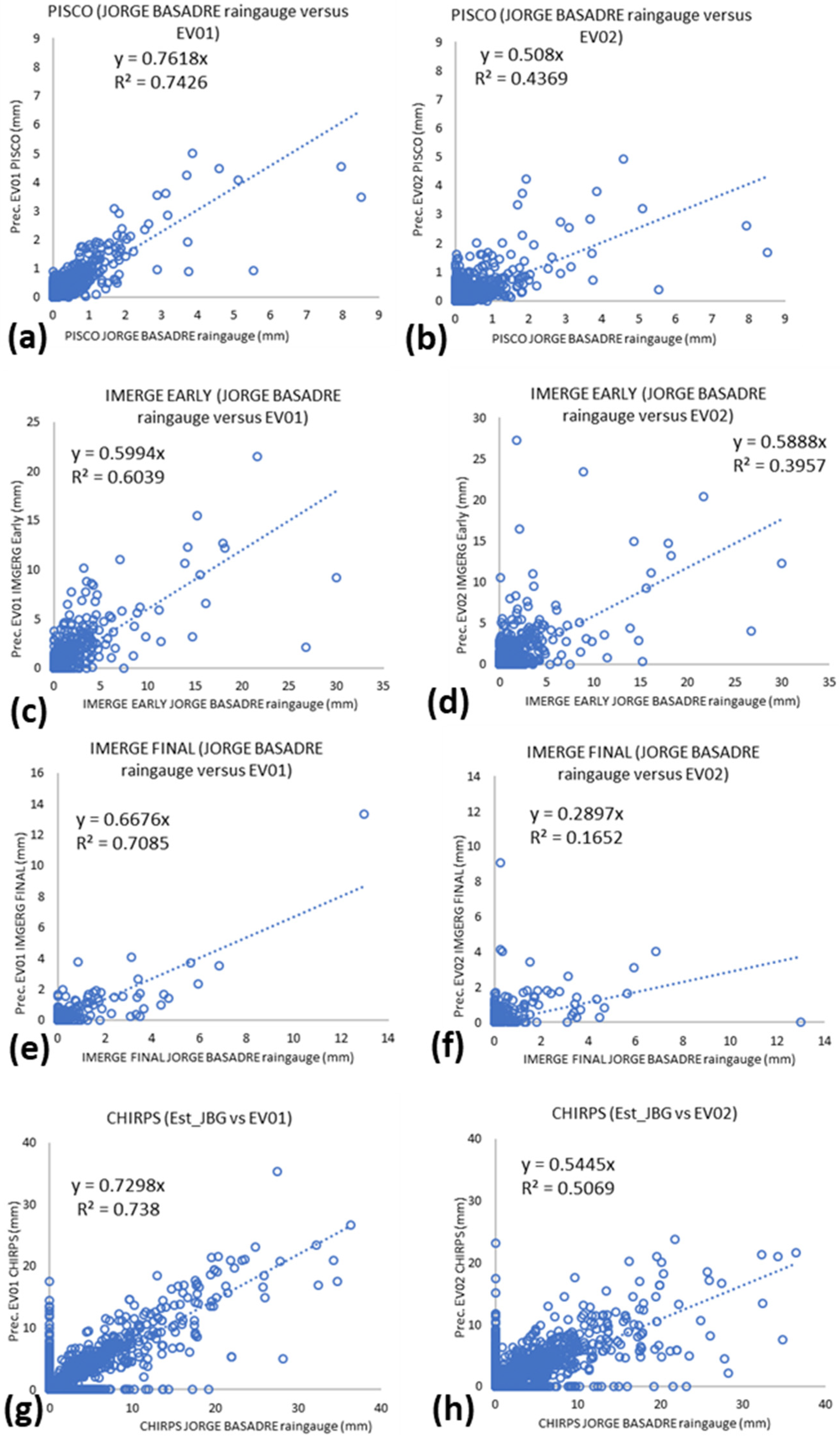
Figure 9.
Correlations were made between the total daily precipitation data between the JORGE BASADRE rain gauge and the virtual rain gauges, (EV01 and EV02) using the products: (a,b) PISCO, (c,d) IMERGE Early, (e,f) IMERGE Final, and (g,h) CHIRPS.
Figure 9.
Correlations were made between the total daily precipitation data between the JORGE BASADRE rain gauge and the virtual rain gauges, (EV01 and EV02) using the products: (a,b) PISCO, (c,d) IMERGE Early, (e,f) IMERGE Final, and (g,h) CHIRPS.
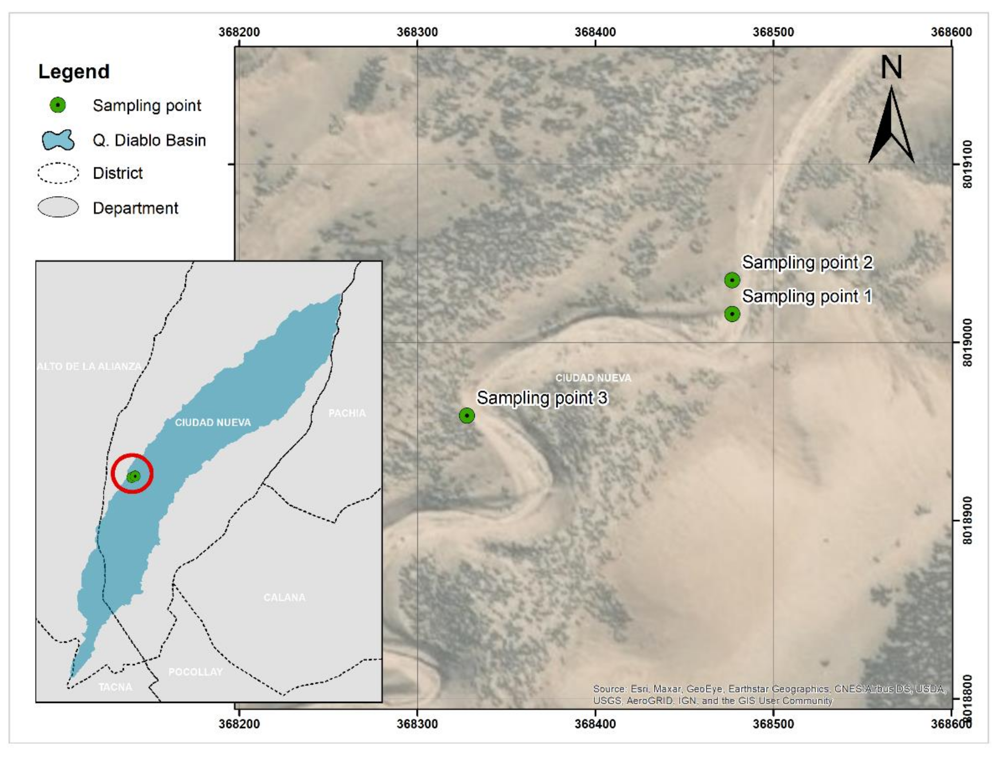
Figure 10.
Location of soil sampling points.
Figure 10.
Location of soil sampling points.
Figure 11.
Composition of the SOCONT model.
Figure 11.
Composition of the SOCONT model.
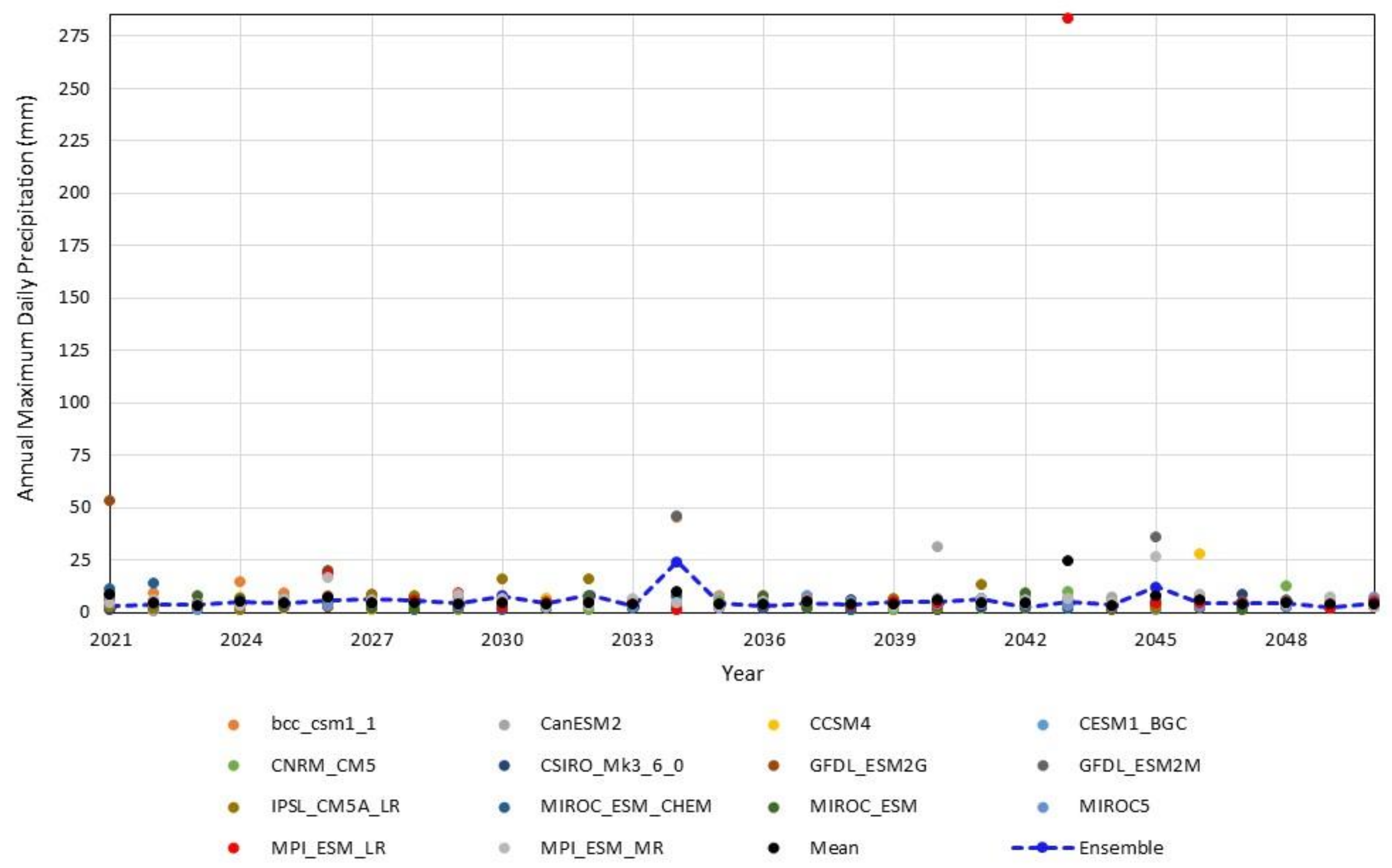
Figure 12.
Annual maximum daily precipitation projected by 14 climate models under the RCP4.5 scenario for the Devil’s Creek. The dashed blue line corresponds to the ensemble. Period: 2021–2050.
Figure 12.
Annual maximum daily precipitation projected by 14 climate models under the RCP4.5 scenario for the Devil’s Creek. The dashed blue line corresponds to the ensemble. Period: 2021–2050.
Figure 13.
Boxplot for future projections of the annual maximum daily precipitation of 14 GCMs under the RCP4.5 scenario in the Devil’s Creek, period 2021–2050. The linear extensions represent the highest and lowest values; the upper, middle and lower limits of the box represent the percentiles of 75%, 50%, and 25%, respectively; and the solid circles represent the outliers.
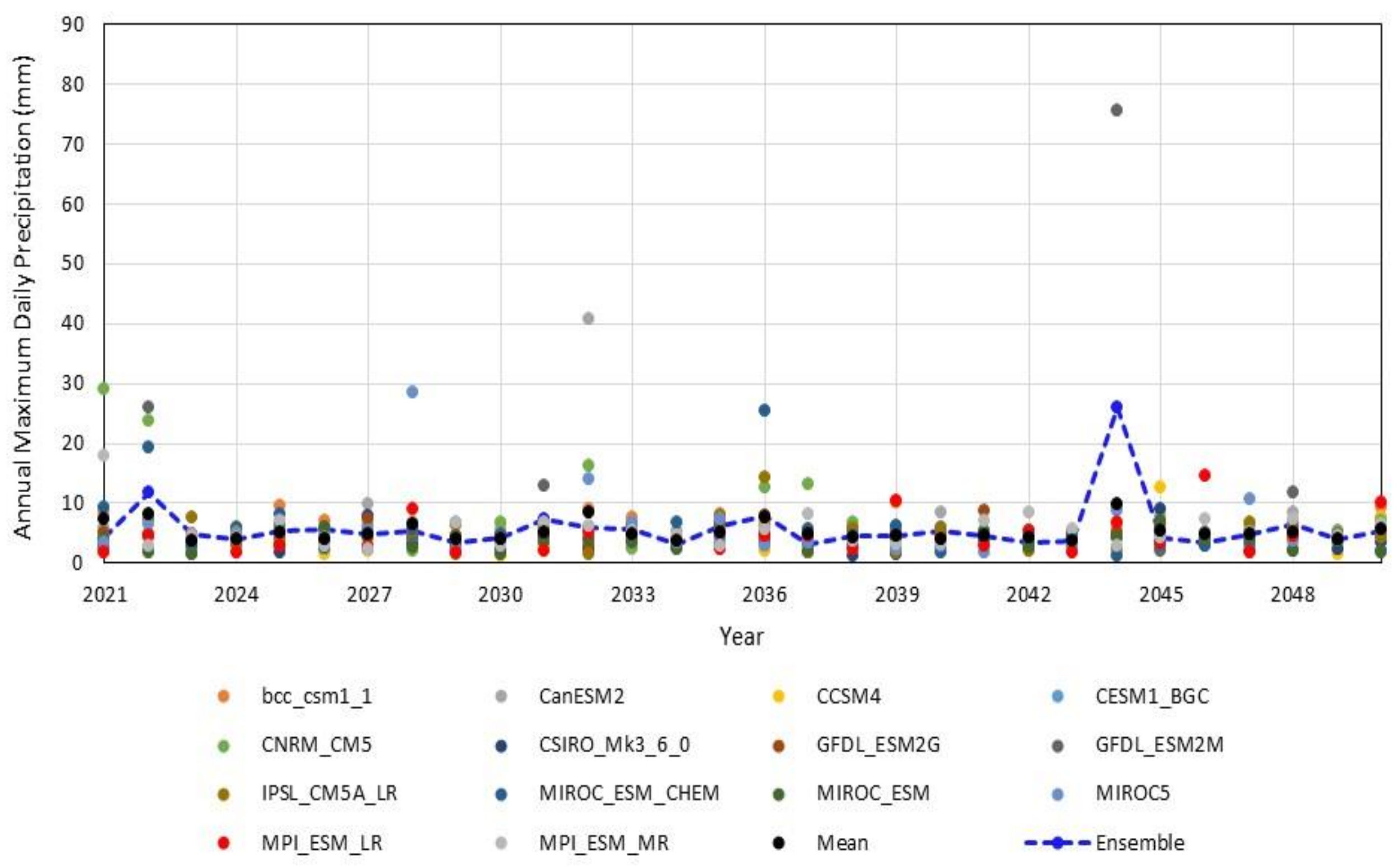
Figure 14.
Annual maximum daily precipitation projected by 14 climate models under the RCP8.5 scenario for the Devil’s Creek. The dashed blue line corresponds to the ensemble. Period: 2021–2050.
Figure 14.
Annual maximum daily precipitation projected by 14 climate models under the RCP8.5 scenario for the Devil’s Creek. The dashed blue line corresponds to the ensemble. Period: 2021–2050.
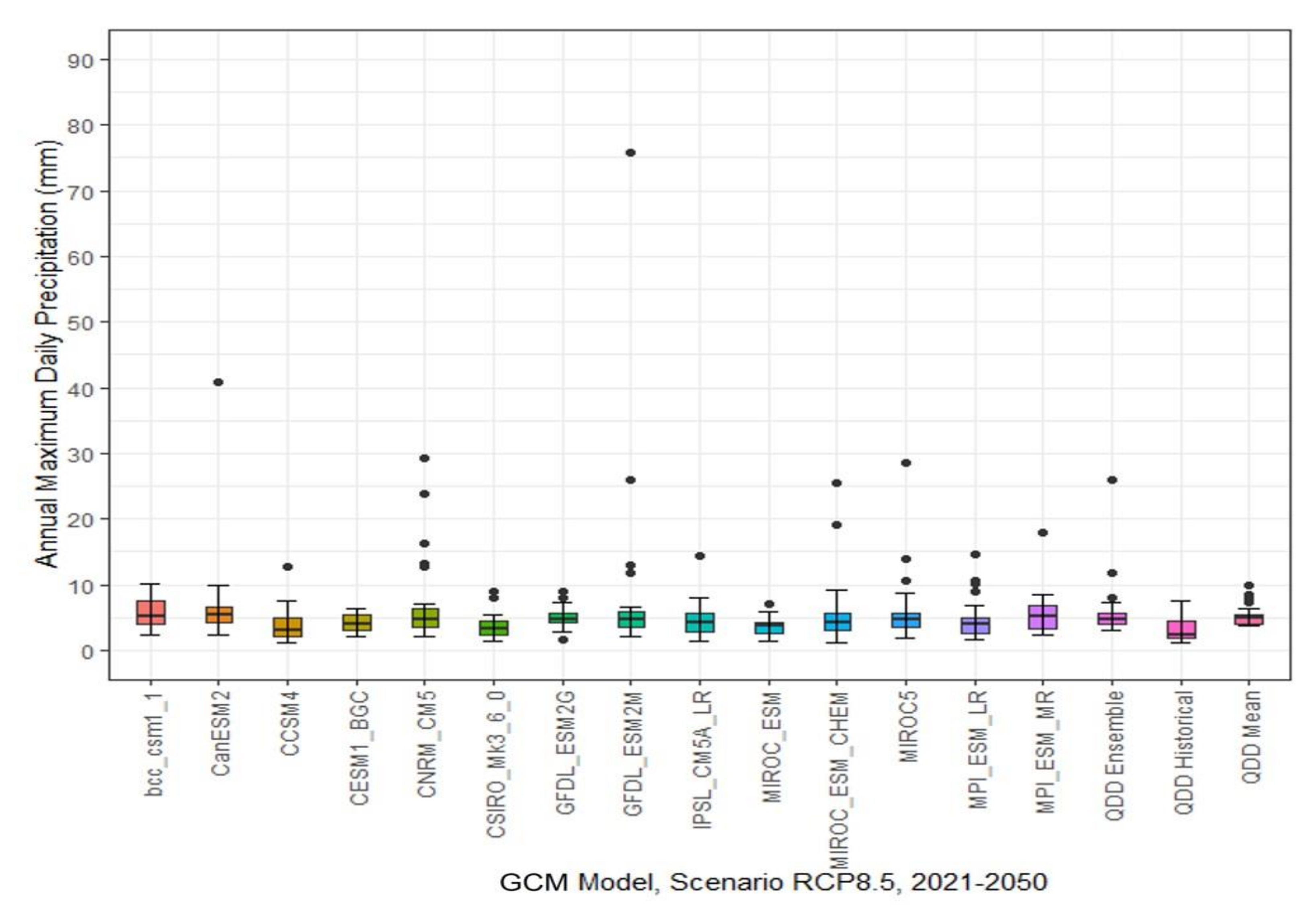
Figure 15.
Boxplot for future projections of the annual maximum daily precipitation of 14 GCMs under the RCP8.5 scenario in the Devil’s Creek, period 2021–2050. The linear extensions represent the highest and lowest values; the upper, middle and lower limits of the box represent the percentiles of 75%, 50%, and 25%, respectively; and the solid circles represent the outliers.
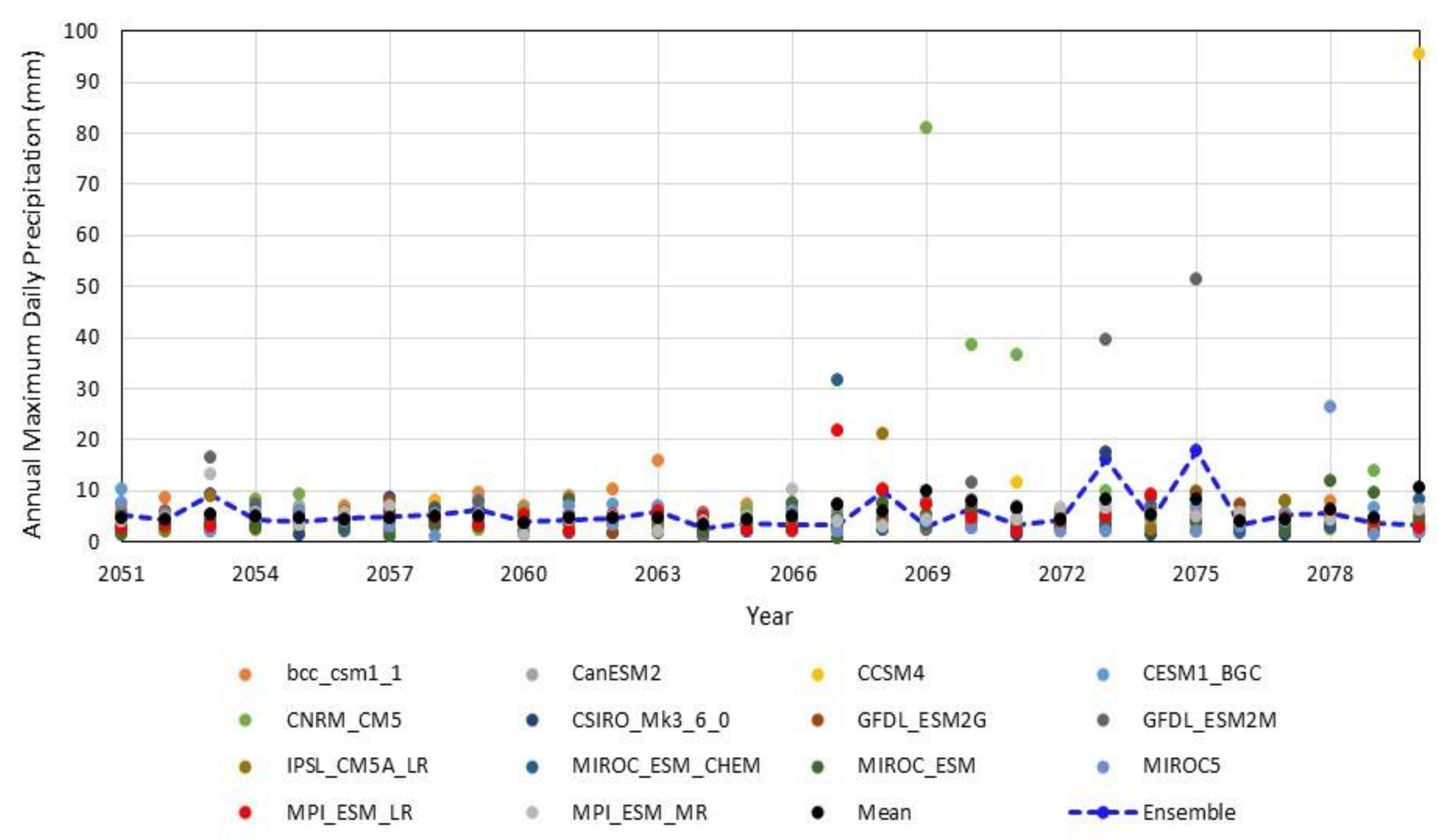
Figure 16.
Annual maximum daily precipitation projected by 14 climate models under the RCP4.5 scenario for Devil’s Creek. The dashed blue line corresponds to the ensemble. Period: 2051–2080.
Figure 16.
Annual maximum daily precipitation projected by 14 climate models under the RCP4.5 scenario for Devil’s Creek. The dashed blue line corresponds to the ensemble. Period: 2051–2080.
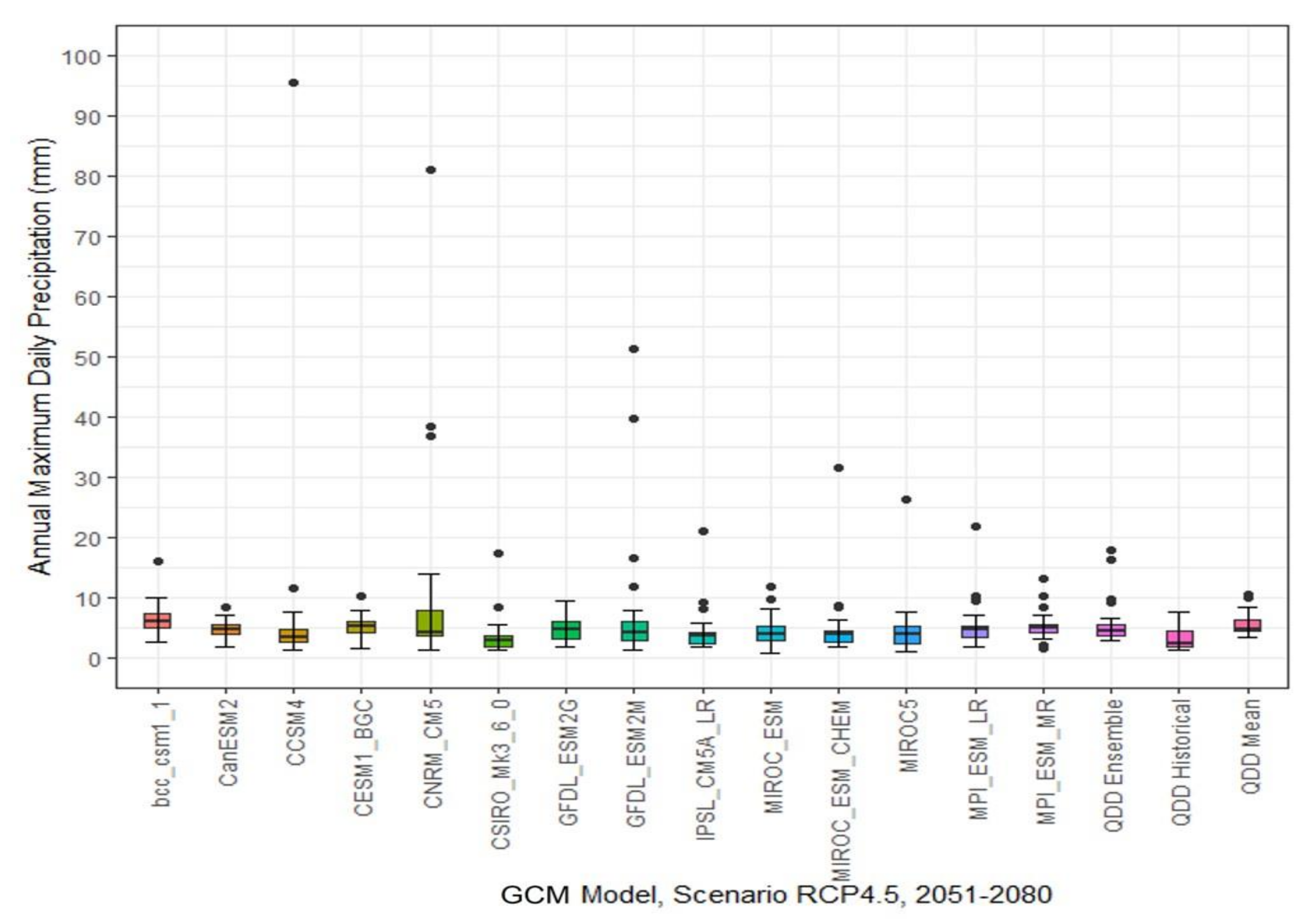
Figure 17.
Boxplot for future projections of the annual maximum daily precipitation of 14 GCMs under the RCP4.5 scenario in the Devil’s Creek, period 2051–2080. The linear extensions represent the highest and lowest values; the upper, middle and lower limits of the box represent the percentiles of 75%, 50%, and 25%, respectively; and the solid circles represent the outliers.
Figure 18.
Annual maximum daily precipitation projected by 14 climate models under the RCP8.5 scenario for the Devil’s Creek. The dashed blue line corresponds to the ensemble. Period: 2051–2080.
Figure 18.
Annual maximum daily precipitation projected by 14 climate models under the RCP8.5 scenario for the Devil’s Creek. The dashed blue line corresponds to the ensemble. Period: 2051–2080.
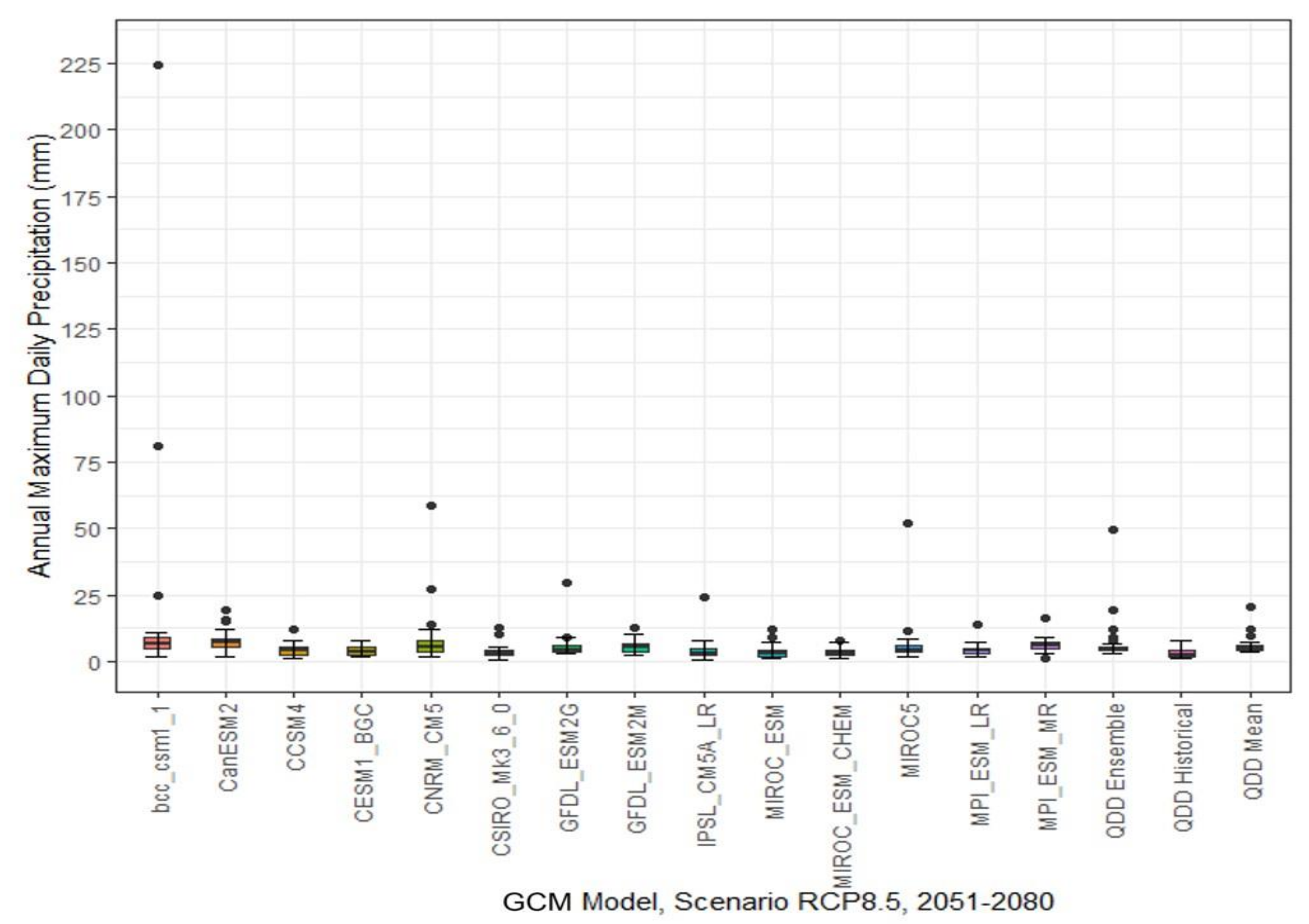
Figure 19.
Boxplot for future projections of the annual maximum daily precipitation of 14 GCMs under the RCP8.5 scenario in the Devil’s Creek, 2051–2080 term. The linear extensions represent the highest and lowest values; the upper, middle, and lower limits of the box represent the percentiles of 75%, 50%, and 25%, respectively; and the solid circles represent the outliers.
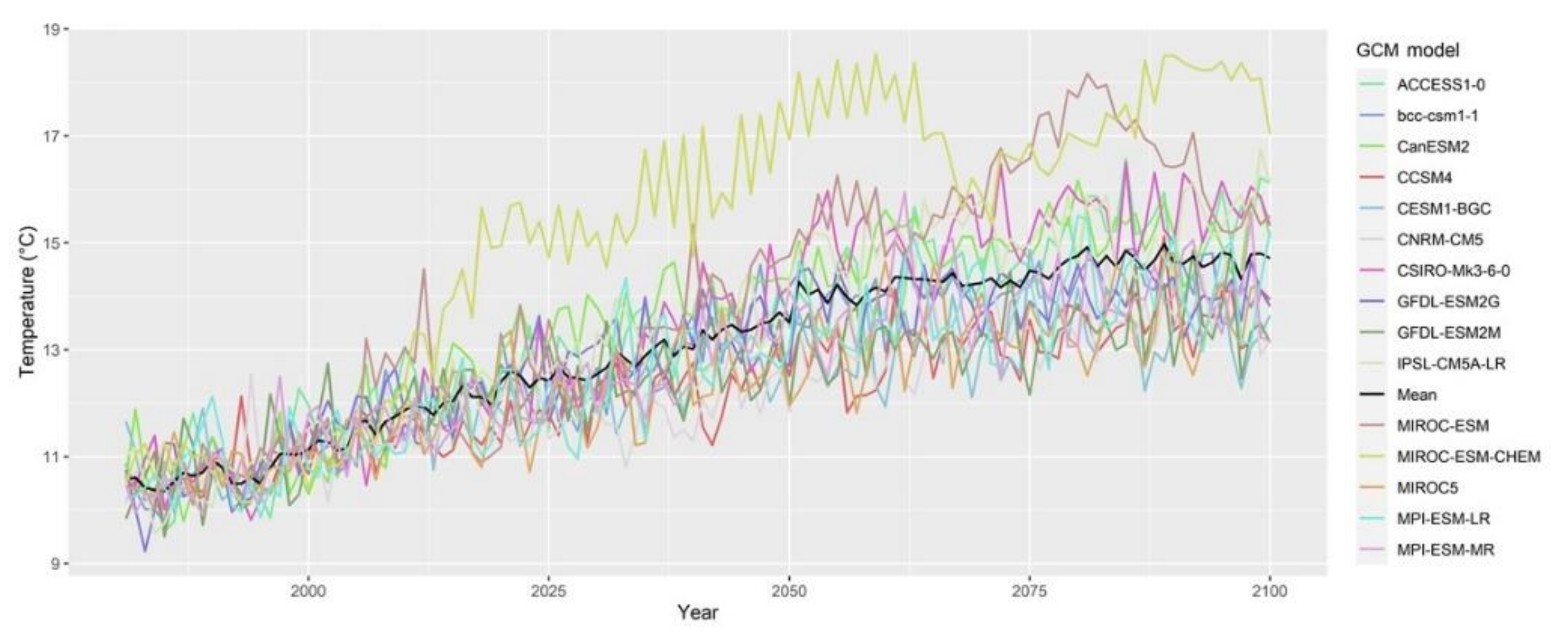
Figure 20.
Minimum annual average temperature simulated by climate models, corrected and scaled for the Devil’s Creek, 1981–2100 term, RCP4.5 emission scenario. The black line represents the averaged ensemble of 15 GCMs.
Figure 20.
Minimum annual average temperature simulated by climate models, corrected and scaled for the Devil’s Creek, 1981–2100 term, RCP4.5 emission scenario. The black line represents the averaged ensemble of 15 GCMs.
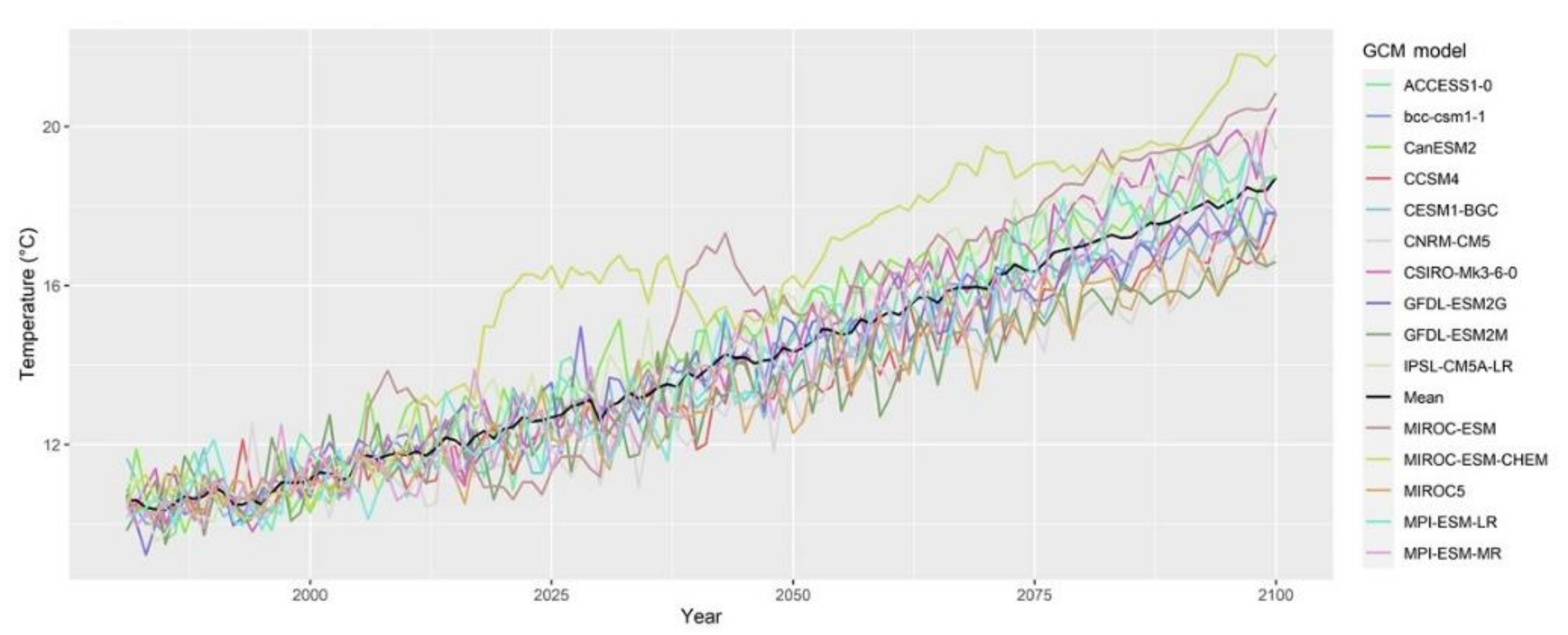
Figure 21.
Minimum annual average temperature simulated by climate models, corrected and scaled for the Devil’s Creek, 1981–2100 term, RCP8.5 emission scenario. The black line represents the averaged ensemble of the 15 GCMs.
Figure 21.
Minimum annual average temperature simulated by climate models, corrected and scaled for the Devil’s Creek, 1981–2100 term, RCP8.5 emission scenario. The black line represents the averaged ensemble of the 15 GCMs.
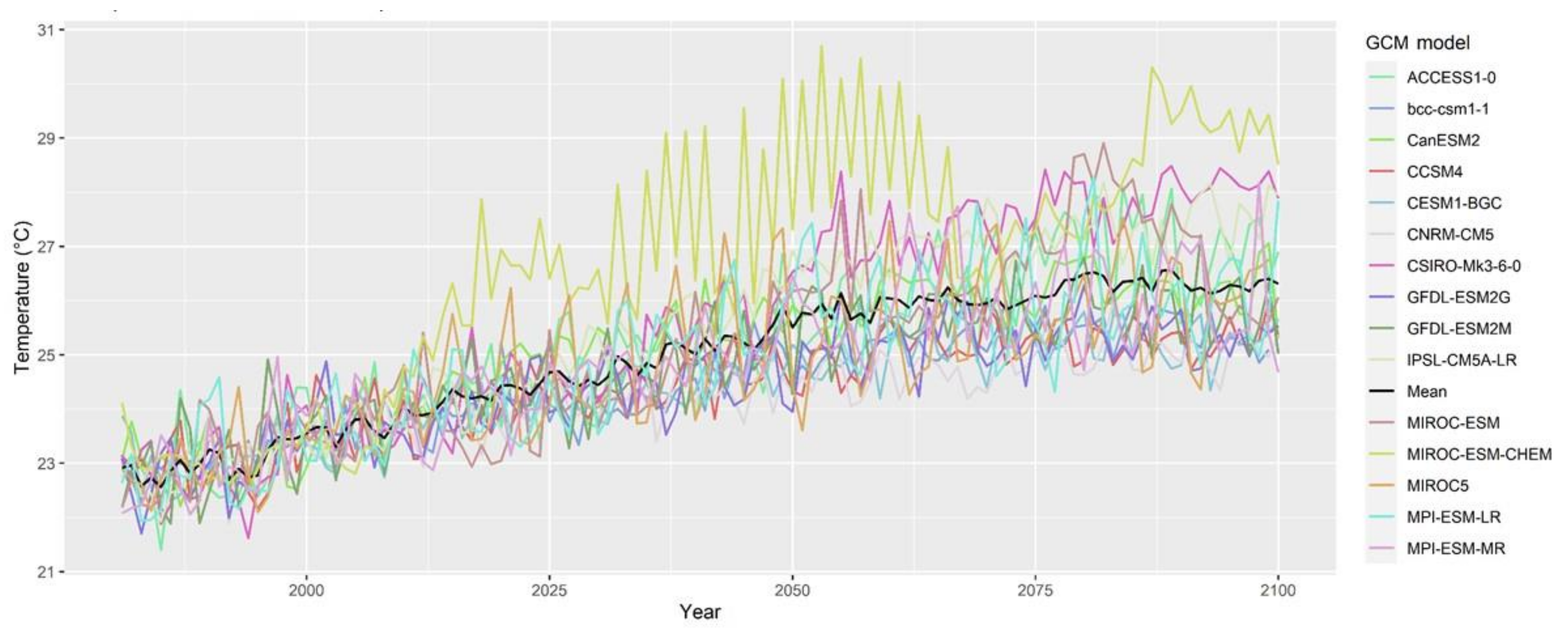
Figure 22.
Maximum annual average temperature simulated by climate models, corrected and scaled for the Devil’s Creek, 1981–2100 term, RCP4.5 emission scenario. The black line represents the averaged ensemble of 15 GCMs.
Figure 22.
Maximum annual average temperature simulated by climate models, corrected and scaled for the Devil’s Creek, 1981–2100 term, RCP4.5 emission scenario. The black line represents the averaged ensemble of 15 GCMs.
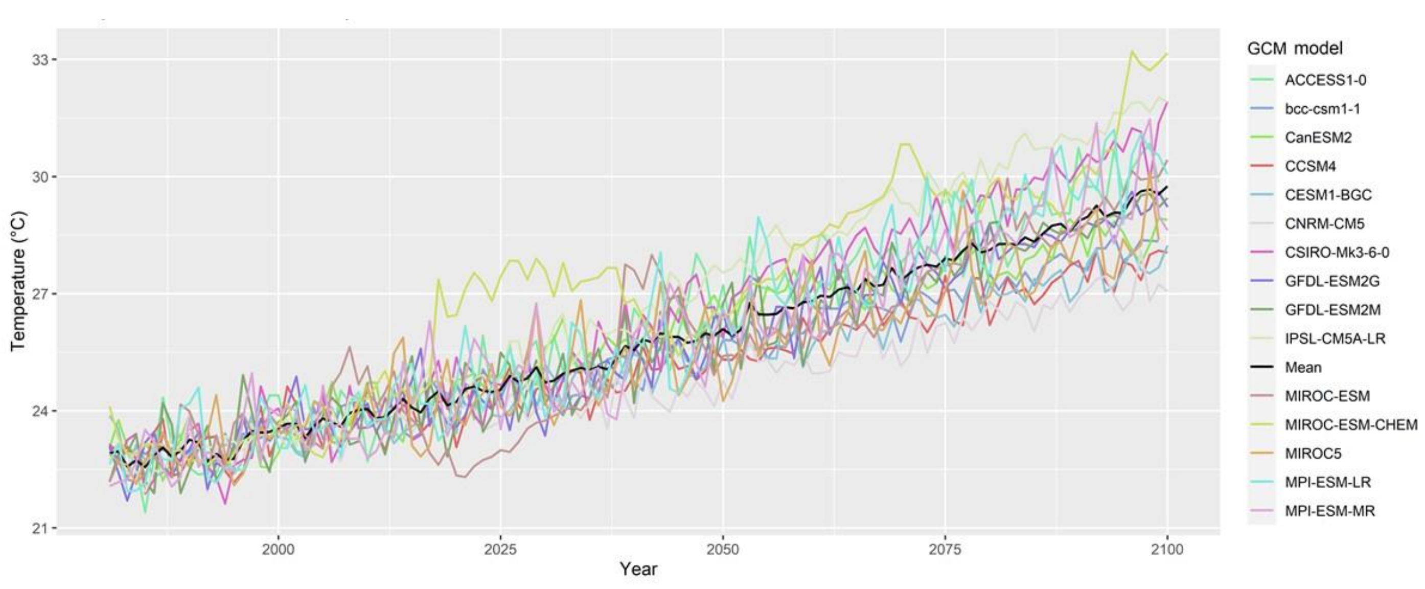
Figure 23.
Maximum annual average temperature simulated by regional climate models, corrected and scaled for the Devil’s Creek, 1981–2100 term, RCP8.5 emission scenario. The black line represents the averaged ensemble of 15 GCMs.
Figure 23.
Maximum annual average temperature simulated by regional climate models, corrected and scaled for the Devil’s Creek, 1981–2100 term, RCP8.5 emission scenario. The black line represents the averaged ensemble of 15 GCMs.
Figure 24.
Average monthly temperature (minimum) under RCP4.5 and RCP8.5 scenarios for the Devil’s Creek, 2021–2050 and 2051–2080 periods. The multi-model ensemble average of 15 GCMs.
Figure 24.
Average monthly temperature (minimum) under RCP4.5 and RCP8.5 scenarios for the Devil’s Creek, 2021–2050 and 2051–2080 periods. The multi-model ensemble average of 15 GCMs.
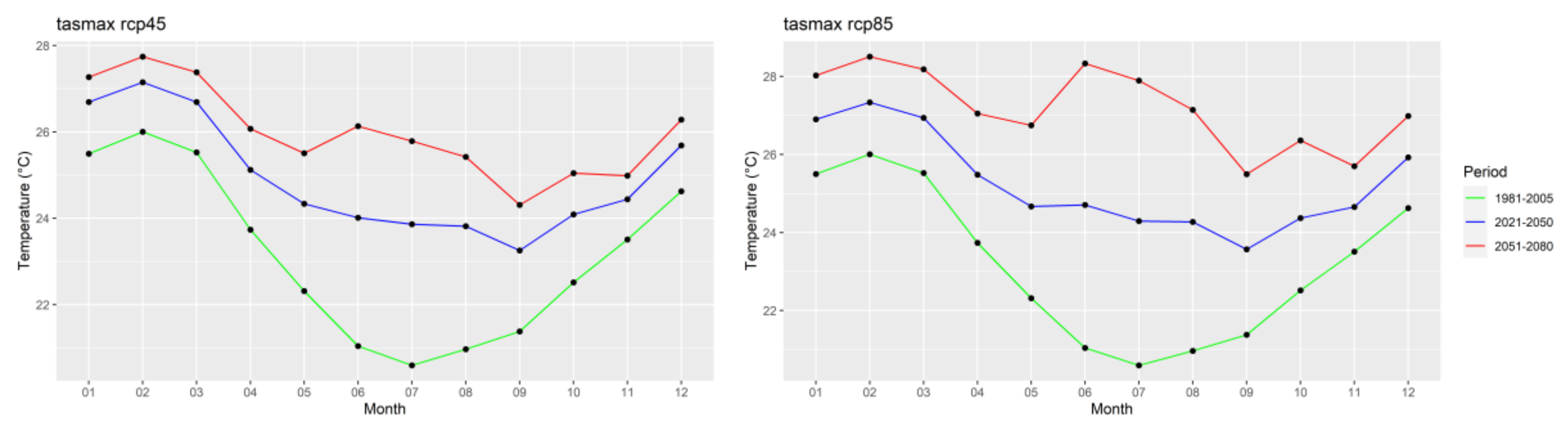
Figure 25.
Average monthly temperature (maximum) under RCP4.5 and RCP8.5 scenarios for the Devil’s Creek, 2021–2050 and 2051–2080 periods. The multi-model ensemble average of 15 GCMs.
Figure 25.
Average monthly temperature (maximum) under RCP4.5 and RCP8.5 scenarios for the Devil’s Creek, 2021–2050 and 2051–2080 periods. The multi-model ensemble average of 15 GCMs.
Figure 26.
Average monthly temperature change (minimum) under RCP4.5 and RCP8.5 scenarios for the Devil’s Creek, 2021–2050 and 2051–2080 periods. The multi-model ensemble average of 15 GCMs.
Figure 26.
Average monthly temperature change (minimum) under RCP4.5 and RCP8.5 scenarios for the Devil’s Creek, 2021–2050 and 2051–2080 periods. The multi-model ensemble average of 15 GCMs.
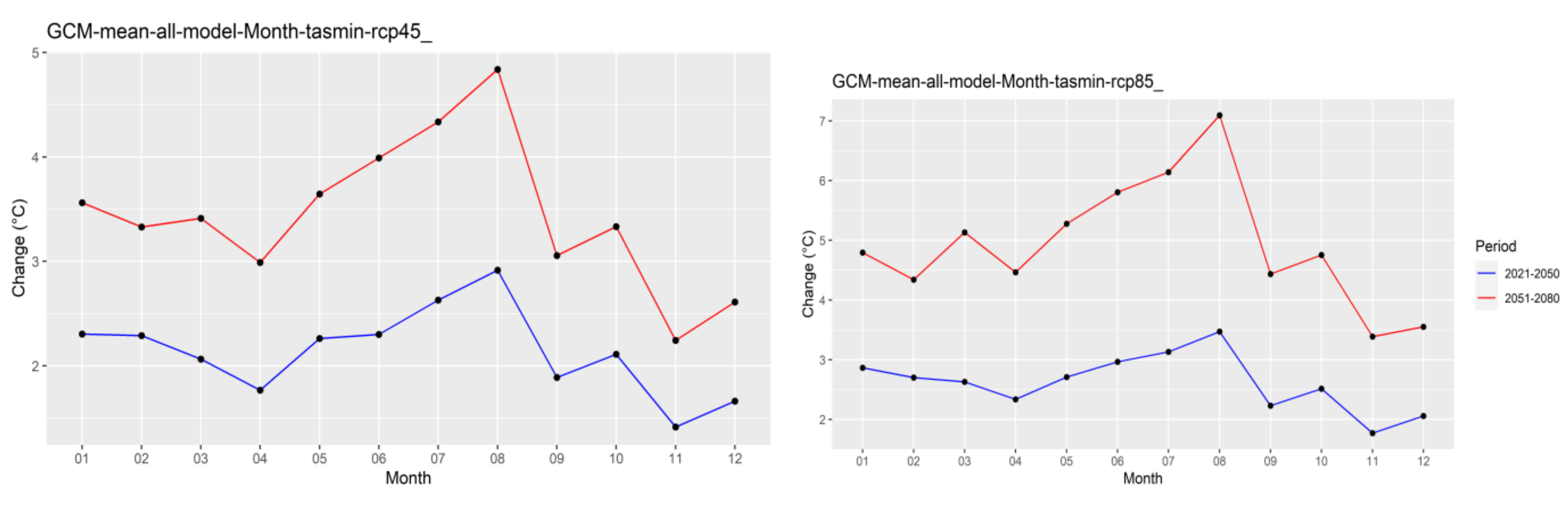
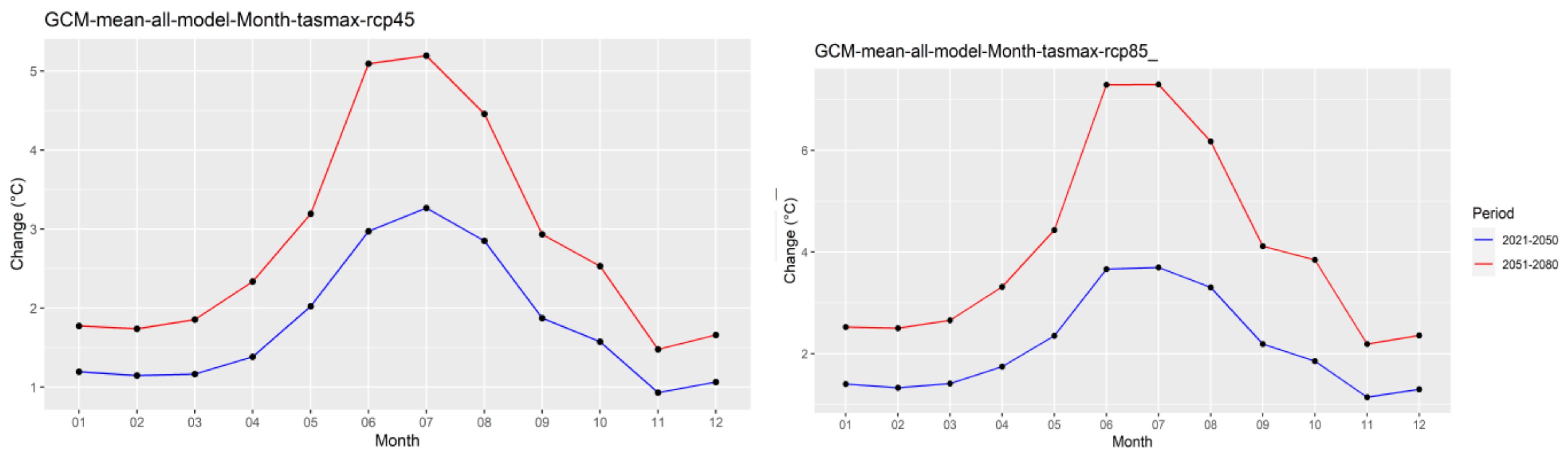
Figure 27.
Average monthly temperature change (maximum) under RCP4.5 and RCP8.5 scenarios for the Devil’s Creek, 2021–2050 and 2051–2080 periods. The multi-model ensemble average of 15 GCMs.
Figure 27.
Average monthly temperature change (maximum) under RCP4.5 and RCP8.5 scenarios for the Devil’s Creek, 2021–2050 and 2051–2080 periods. The multi-model ensemble average of 15 GCMs.
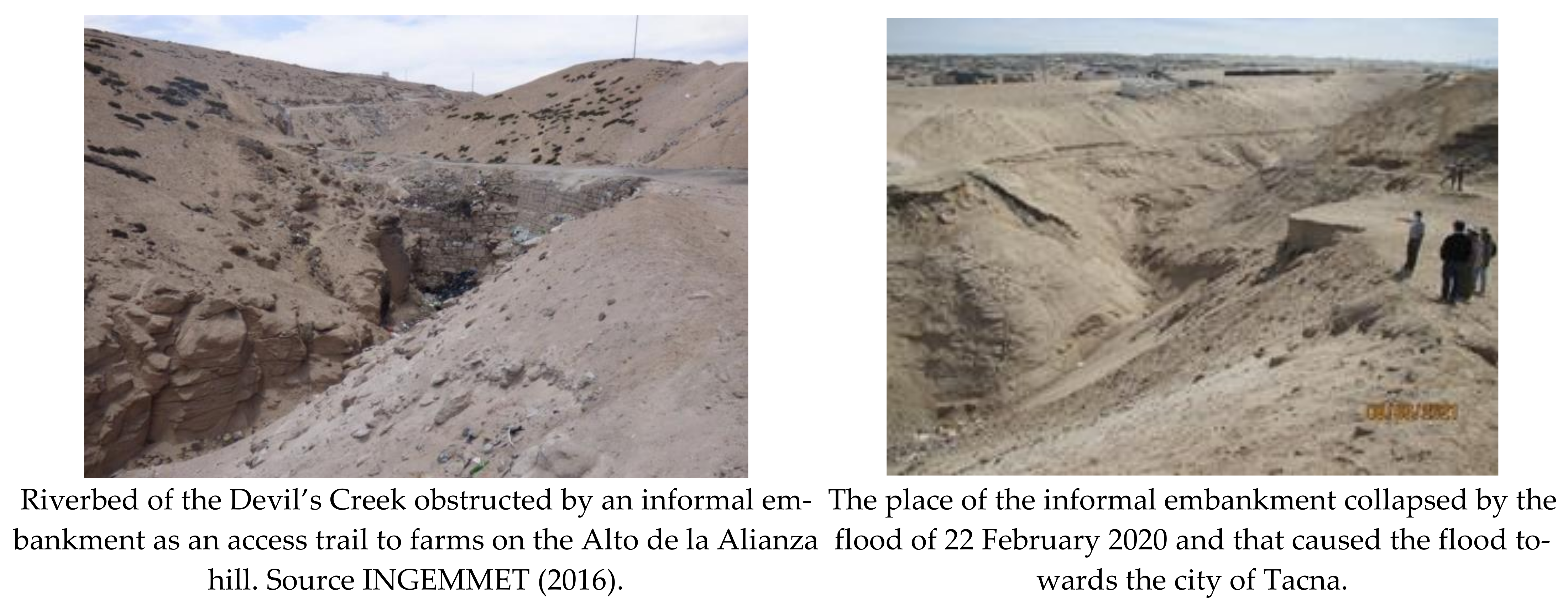
Figure 28.
Before and after the Devil’s Creek channel was obstructed by an informal embankment as an access trail to farms in the Alto de la Alianza hill.
Figure 28.
Before and after the Devil’s Creek channel was obstructed by an informal embankment as an access trail to farms in the Alto de la Alianza hill.
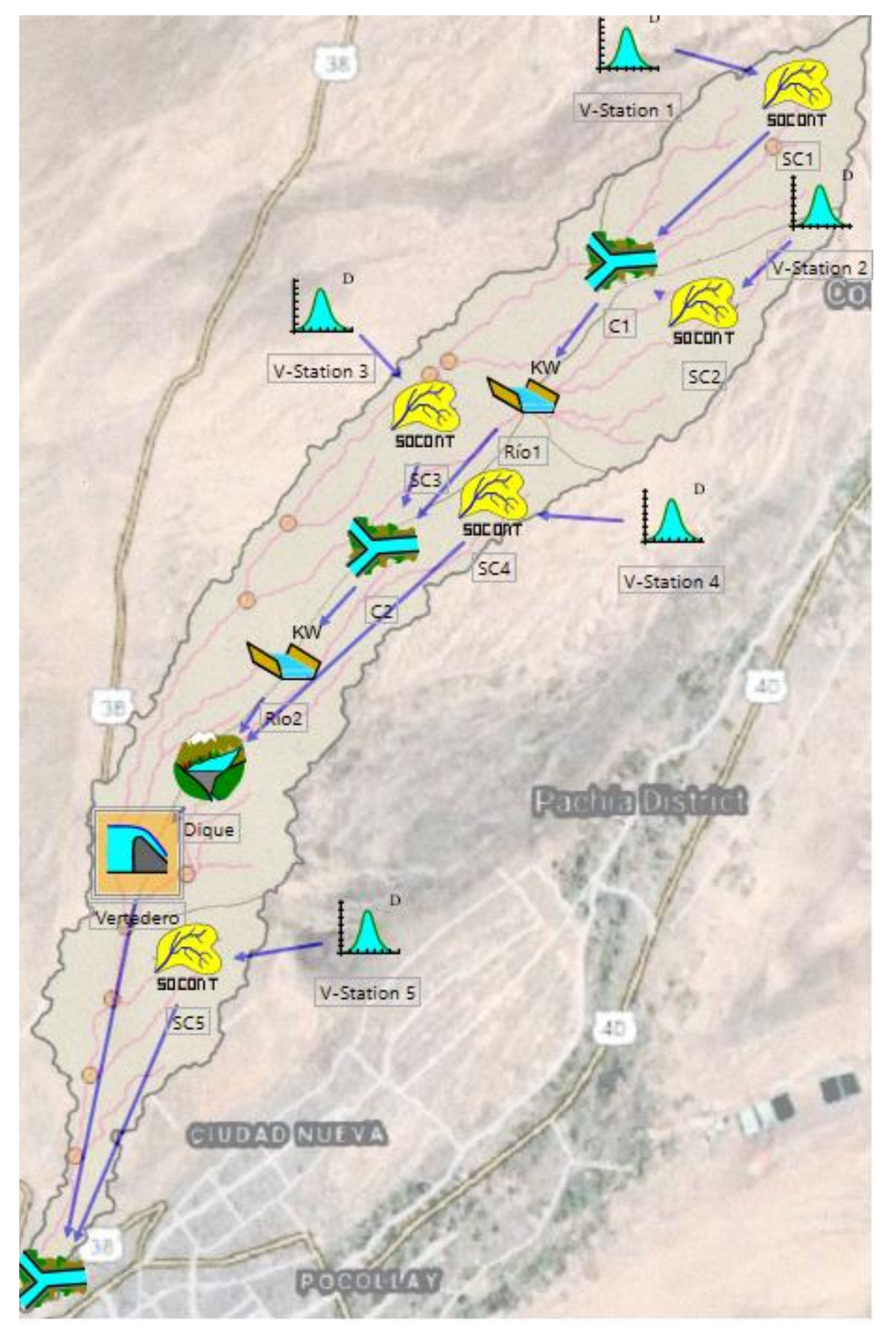
Figure 29.
Structure of the RS Minerve Model for simulation of the 21 February 2020 event.
Figure 29.
Structure of the RS Minerve Model for simulation of the 21 February 2020 event.
Figure 30.
Sea surface temperature anomalies between 1 December 2019 and 28 March 2020.
Figure 30.
Sea surface temperature anomalies between 1 December 2019 and 28 March 2020.
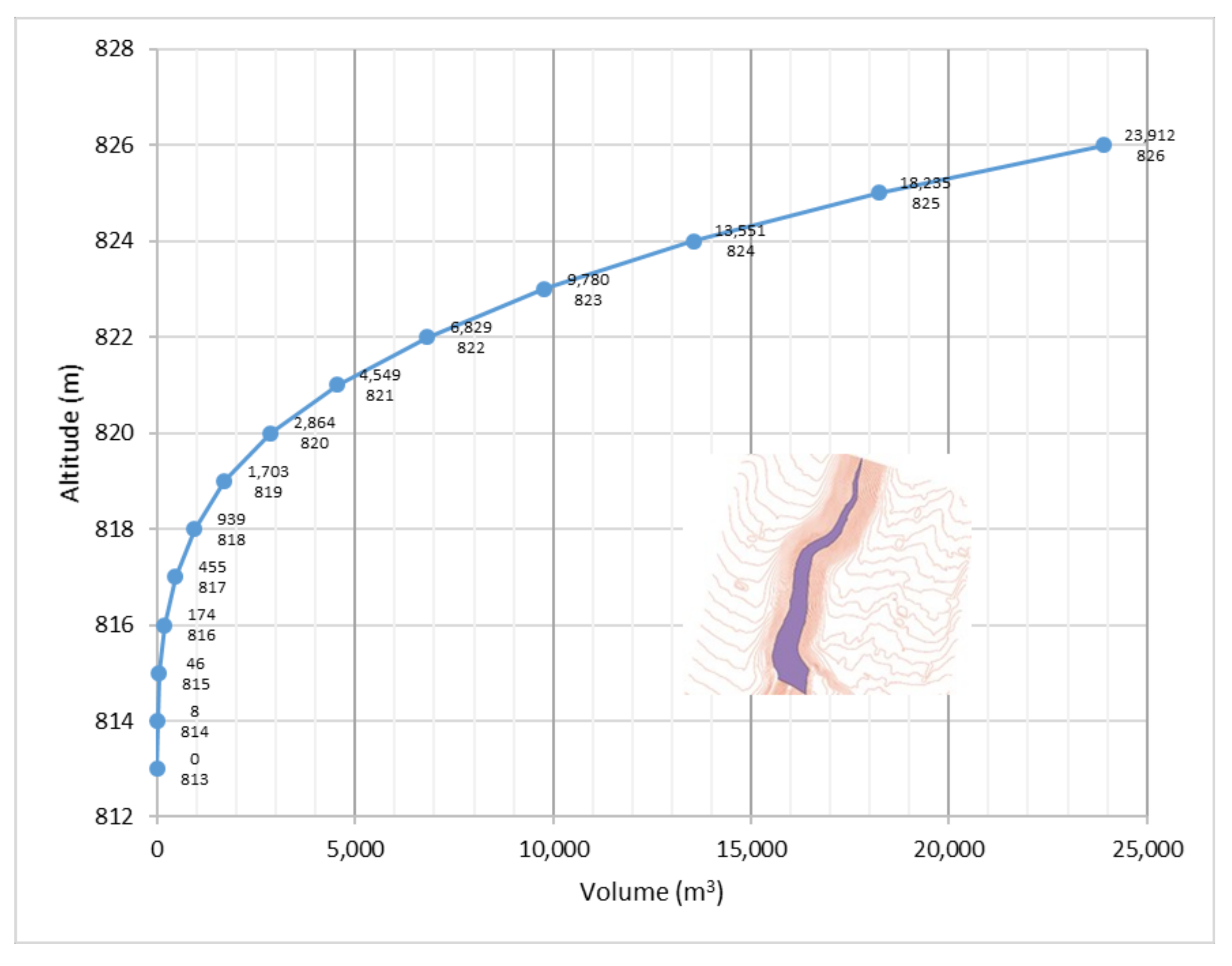
Figure 31.
Bathymetry of the informal Paso Camiara embankment.
Figure 31.
Bathymetry of the informal Paso Camiara embankment.
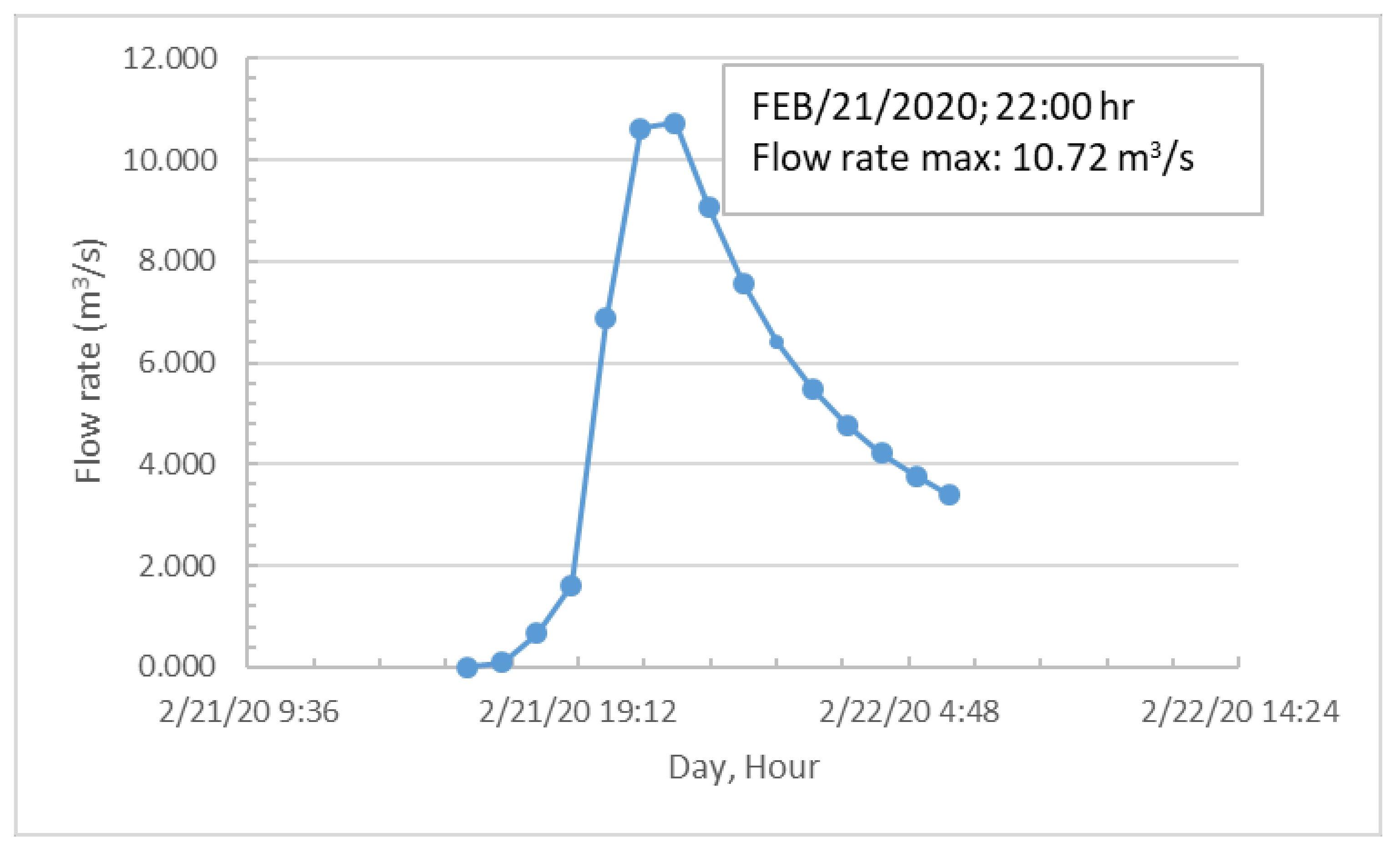
Figure 32.
Hydrographs generated by the sub-basins.
Figure 32.
Hydrographs generated by the sub-basins.
Figure 33.
Hydrograph of entry to the Paso Camiara informal embankment.
Figure 33.
Hydrograph of entry to the Paso Camiara informal embankment.
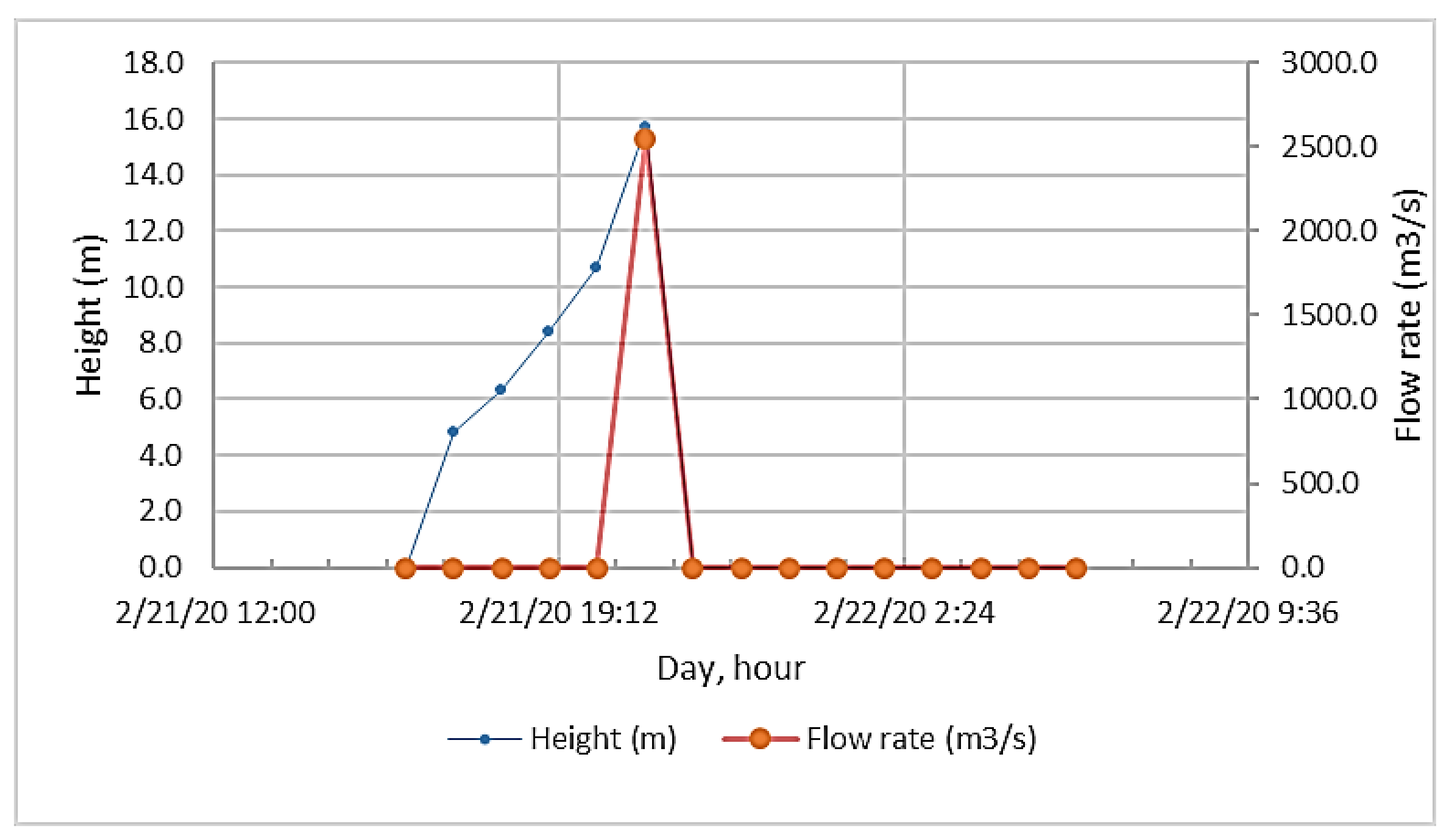
Figure 34.
Hydrographs of water height in the dam and flow discharged due to the collapse of the Paso Camiara dam.
Figure 34.
Hydrographs of water height in the dam and flow discharged due to the collapse of the Paso Camiara dam.
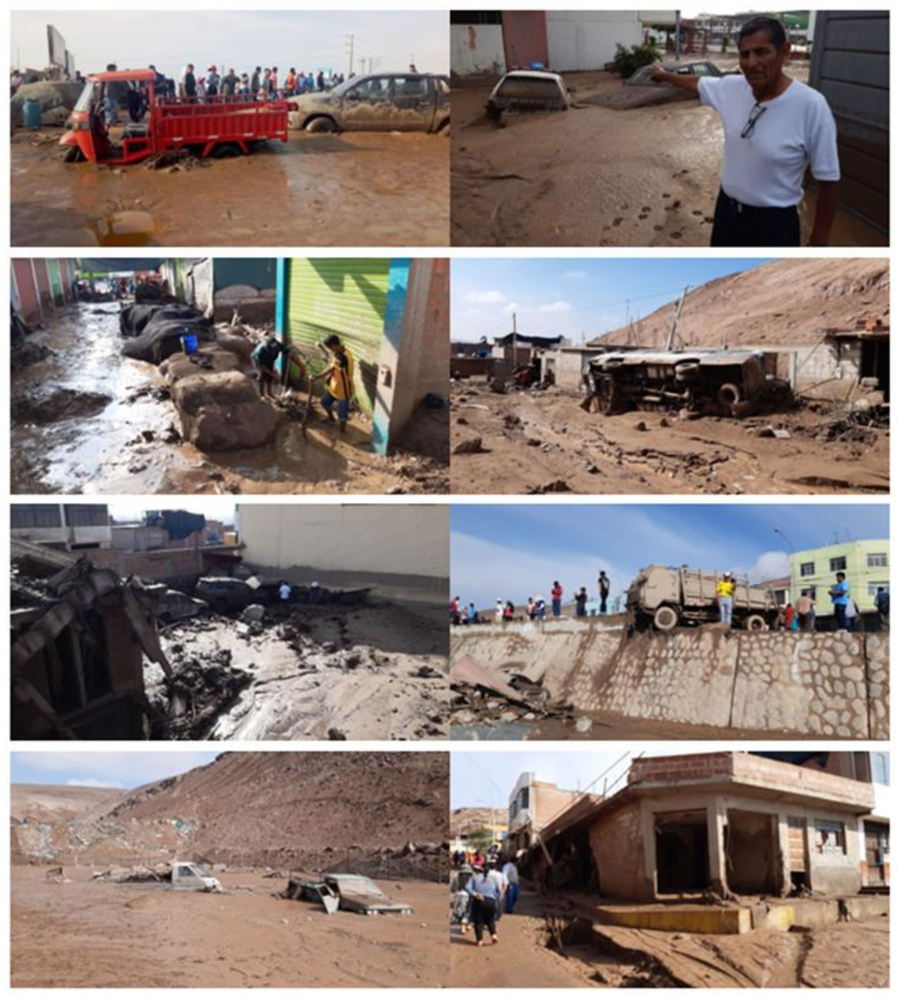
Figure 35.
Gestion newspaper reports: debris flow in Tacna left three people dead, 22 February 2020.
Figure 35.
Gestion newspaper reports: debris flow in Tacna left three people dead, 22 February 2020.
Figure 36.
Structure of the RS Minerve Model for the simulations of events with different climate change scenarios.
Figure 36.
Structure of the RS Minerve Model for the simulations of events with different climate change scenarios.
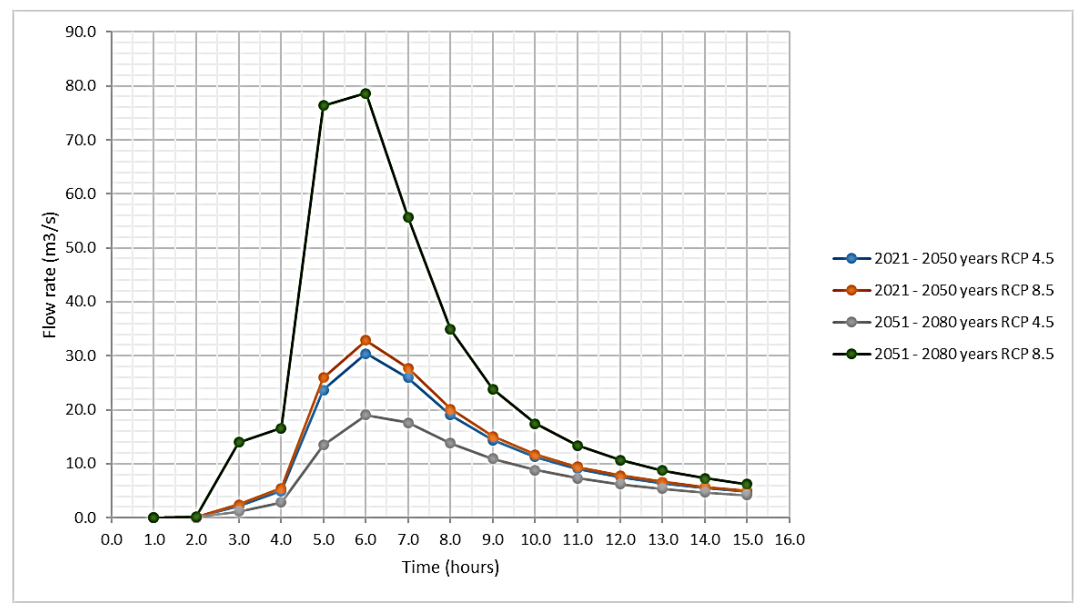
Figure 37.
Flood hydrographs for RCP4.5 and RCP8.5 scenarios for 2021–2050 and 2051–2080 terms.
Figure 37.
Flood hydrographs for RCP4.5 and RCP8.5 scenarios for 2021–2050 and 2051–2080 terms.
Table 1.
Availability of precipitation data.
Table 1.
Availability of precipitation data.
| Rain Gauge | No. Values | Start Date | Final Date | % Gaps | Duration (Years) |
|---|
| Calana | 19,704 | 1 January 1966 | 31 December 2020 | 2 | 55 |
| JORGE BASADRE | 9952 | 1 January 1993 | 31 December 2020 | 3 | 28 |
| Calientes | 19,298 | 1 January 1966 | 31 December 2020 | 4 | 55 |
| Sama Grande | 19,789 | 1 January 1966 | 31 December 2020 | 1 | 55 |
| Palca | 15,866 | 1 July 1966 | 31 December 2020 | 20 | 55 |
Table 2.
Virtual rain gauges and JORGE BASADRE rain gauge.
Table 2.
Virtual rain gauges and JORGE BASADRE rain gauge.
| No | Rain Gauge | Length | Latitude | Elevation (masl) | Source | Record |
|---|
| 1 | Jorge Basadre G. | −70.2515° | −18.0268° | 552 | UNJBG | 1993–2014,
2017–2021 |
| 2 | EV01 | −70.25° | −17.95° | 941 | - | - |
| 5 | EV02 | −70.15° | −17.85° | 1560 | - | - |
Table 3.
Satellite and data base products analyzed.
Table 3.
Satellite and data base products analyzed.
| Product | Version | Abbreviation | Source | Resolution | Frequency | Term |
|---|
| Peruvian Interpolated data of SENAMHI’s Climatological and Hydrological Observations | V. 2.1 | PISCO | SENAMHI | 0.1° × 0.1° | Daily | 1981–2016 |
| Integrated Multi-satellite Retrievals for GPM | Early V06B | IMERG-F | NASA | 0.1° × 0.1° | Daily and 30 min | 2000–2021 |
| Integrated Multi-satellite Retrievals for GPM | Final V06B | IMERG-E | NASA | 0.1° × 0.1° | Daily and 30 min | 2000–2021 |
| Climate Hazards group Infrared Precipitation with Rain gauges | V. 2.0 | CHIRPS | UCSB (x) | 0.05° × 0.05° | Daily | 1981–2021 |
Table 4.
Summary of the regression coefficients and percentage between the JORGE BASADRE rain gauge and the virtual rain gauge (EV01 and EV02).
Table 4.
Summary of the regression coefficients and percentage between the JORGE BASADRE rain gauge and the virtual rain gauge (EV01 and EV02).
| Virtual Rain Gauge | PISCO JB Rain Gauge | IMERG Early JB Rain Gauge | IMERG Final JB Rain Gauge | CHIRPS JB Rain Gauge | Mean | EV01 and EV02 Have Less Precipitation than JORGE BASADRE Rain Gauge
(%) |
|---|
| EV01 | 0.76 | 0.60 | 0.67 | 0.73 | 0.69 | 100% − 69% = 31.0% |
| EV02 | 0.51 | 0.59 | 0.29 | 0.54 | 0.483 | 100% − 48.3% = 51.7% |
Table 5.
Location of sampling points, texture, infiltration equation, and hydraulic conductivity at saturation (Ks).
Table 5.
Location of sampling points, texture, infiltration equation, and hydraulic conductivity at saturation (Ks).
| Sampling | UTM Coordinates | Texture | Infiltration Equation
F (mm), t (min) | Ks
(mm/min) |
|---|
| 1 | 368477E, 8019016N | Clayey silt | F = 4.0 t0.81 | 0.872 |
| 2 | 368477E, 8019035N | Sandy silt with gravel and clay | F = 3.67 t0.87 | 1311 |
| 3 | 368328E, 8018959N | Sandy silt with gravels | F = 7.2 t0.72 | 0.749 |
Table 6.
SOCONT model parameters and plugins [
45].
Table 6.
SOCONT model parameters and plugins [
45].
| Object | Name | Units | Description | Regular Range |
|---|
| SOCONT | A | m2 | Surface | >0 |
| S | mm/°C/d | Reference degree-day snowmelt coefficient | 0.5 to 20 |
| SInt | mm/°C/d | Degree-day snowmelt coefficient | 0 to 4 |
| Smin | mm/°C/d | Minimal degree-day snowmelt coefficient | ≥0 |
| SPh | d | Phase shift of the sinusoidal function | 1 to 365 |
| ThetaCri | - | Critical relative water content of the snow pack | 0.1 |
| bp | d/mm | Melt coefficient due to liquid precipitation | 0.0125 |
| Tcp1 | °C | Minimum critical temperature for liquid precipitation | 0 |
| Tcp2 | °C | Maximum critical temperature for solid precipitation | 4 |
| Tcf | °C | Critical snowmelt temperature | 0 |
| HGR3Max | m | Maximum height of infiltration reservoir | 0 to 2 |
| KGR3 | 1/s | Release coefficient of infiltration reservoir | 0.00025 to 0.1 |
| L | m | Length of the plane | >0 |
| J0 | - | Runoff slope | >0 |
| Kr | m1/3/s | Strickler coefficient | 0.1 to 90 |
| CFR | - | Refreezing coefficient | 0 to 1 |
| SWEIni | m | Initial snow water equivalent height | - |
| HGR3Ini | m | Initial level in infiltration reservoir | - |
| HrIni | m | Initial runoff water level downstream of the surface | - |
| ThetaIni | - | Initial relative water content in the snow pack | - |
Table 7.
The intensity of precipitation over each sub-basin (mm/h).
Table 7.
The intensity of precipitation over each sub-basin (mm/h).
| Date Hour | SC5 | SC4 and SC3 | SC2 and SC1 |
|---|
| 21 February 2020 15:00 | 0.00 | 0.00 | 0.00 |
| 21 February 2020 16:00 | 0.43 | 0.39 | 0.34 |
| 21 February 2020 17:00 | 2.03 | 1.83 | 1.62 |
| 21 February 2020 18:00 | 1.01 | 0.91 | 0.81 |
| 21 February 2020 19:00 | 5.36 | 4.82 | 4.29 |
| 21 February 2020 20:00 | 2.46 | 2.21 | 1.97 |
| 21 February 2020 21:00 | 0.86 | 0.77 | 0.69 |
| 21 February 2020 22:00 | 0.00 | 0.00 | 0.00 |
Table 8.
SOCONT model parameters for each sub-basin.
Table 8.
SOCONT model parameters for each sub-basin.
| Sub-Basins | SC1 | SC2 | SC3 | SC4 | SC5 |
|---|
| SOCONT Model Parameters |
|---|
| A | m2 | 8,446,871 | 7,775,105 | 16,991,236 | 8,542,694 | 11,086,674 |
| bp | d/mm | 0.0125 | 0.0125 | 0.0125 | 0.0125 | 0.0125 |
| CFR | - | 1 | 1 | 1 | 1 | 1 |
| HGR3Max | m2 | 0.1 | 0.1 | 0.1 | 0.2 | 0.5 |
| J0 | - | 0.102 | 0.060 | 0.028 | 0.036 | 0.047 |
| KGR3 | 1/s | 0.001 | 0.001 | 0.001 | 0.001 | 0.001 |
| Kr | m1/3/s | 2 | 2 | 2 | 2 | 2 |
| L | m | 1489.2 | 1301.7 | 1514.2 | 1008.1 | 1613.8 |
| S | mm/°C/d | 5 | 5 | 5 | 5 | 5 |
| Sint | mm/°C/d | 0 | 0 | 0 | 0 | 0 |
| Smin | mm/°C/d | 0 | 0 | 0 | 0 | 0 |
| SPh | d | 80 | 80 | 80 | 80 | 80 |
| Tcf | °C | 0 | 0 | 0 | 0 | 0 |
| Tcp1 | °C | 0 | 0 | 0 | 0 | 0 |
| Tcp2 | °C | 4 | 4 | 4 | 4 | 4 |
| ThetaCri | - | 0.1 | 0.1 | 0.1 | 0.1 | 0.1 |
| Initial conditions |
| SWEIni | m | 0 | 0 | 0 | 0 | 0 |
| ThetaIni | - | 0 | 0 | 0 | 0 | 0 |
| HGR3Ini | m | 0.1 | 0.1 | 0.1 | 0.1 | 0.1 |
| HrIni | m | 0 | 0 | 0 | 0 | 0 |
Table 9.
Riverbed model parameters by cinematic approximation.
Table 9.
Riverbed model parameters by cinematic approximation.
| Riverbed | River 1 | River 2 |
|---|
| Parameters |
|---|
| L | m | 12,541.4 | 8622.1 |
| B0 | m | 5 | 12 |
| m | - | 1 | 1 |
| J0 | - | 0.03 | 0.0335 |
| K | m1/3/s | 30 | 30 |
| N | - | 1 | 1 |
| Initial conditions |
| Qini | m3/s | 0 | 0 |
Table 10.
Instantaneous discharge flow due to breach of the Paso Camiara informal embankment.
Table 10.
Instantaneous discharge flow due to breach of the Paso Camiara informal embankment.
| Paso Camiara Dam | Hc (m) | V (Hm3) | b (m) | Qp (m3/s) |
| 13 | 0.0239115 | 9.8 | 688.7 |
Table 11.
Precipitation intensity over each sub-basin (mm/h) for RCP4.5 and 8.5 scenarios, from 2021 to 2050 and from 2051 to 2080.
Table 11.
Precipitation intensity over each sub-basin (mm/h) for RCP4.5 and 8.5 scenarios, from 2021 to 2050 and from 2051 to 2080.
| | 2021–2050 (RCP4.5) | 2051–2080 (RCP4.5) | 2021–2050 (RCP8.5) | 2051–2080 (RCP8.5) |
|---|
| Hours | SC5 | SC4 and SC3 | SC2 and SC1 | SC5 | SC4 and SC3 | SC2 and SC1 | SC5 | SC4 and SC3 | SC2 and SC1 | SC5 | SC4 and SC3 | SC2 and SC1 |
|---|
| 0 | 0.00 | 0.00 | 0.00 | 0.00 | 0.00 | 0.00 | 0.00 | 0.00 | 0.00 | 0.00 | 0.00 | 0.00 |
| 1 | 0.87 | 0.78 | 0.70 | 0.63 | 0.57 | 0.51 | 0.92 | 0.83 | 0.73 | 1.76 | 1.58 | 1.41 |
| 2 | 4.11 | 3.70 | 3.29 | 2.98 | 2.69 | 2.39 | 4.34 | 3.90 | 3.47 | 8.31 | 7.48 | 6.65 |
| 3 | 2.04 | 1.84 | 1.64 | 1.48 | 1.34 | 1.19 | 2.16 | 1.94 | 1.73 | 4.13 | 3.72 | 3.31 |
| 4 | 10.85 | 9.77 | 8.68 | 7.88 | 7.09 | 6.30 | 11.45 | 10.31 | 9.16 | 21.94 | 19.75 | 17.55 |
| 5 | 4.98 | 4.48 | 3.98 | 3.62 | 3.25 | 2.89 | 5.26 | 4.73 | 4.20 | 10.07 | 9.06 | 8.06 |
| 6 | 1.74 | 1.57 | 1.39 | 1.26 | 1.14 | 1.01 | 1.84 | 1.65 | 1.47 | 3.52 | 3.17 | 2.82 |
| 7 | 0.00 | 0.00 | 0.00 | 0.00 | 0.00 | 0.00 | 0.00 | 0.00 | 0.00 | 0.00 | 0.00 | 0.00 |
| Total in 6 h | 24.60 | 22.14 | 19.68 | 17.86 | 16.07 | 14.29 | 25.96 | 23.36 | 20.77 | 49.74 | 44.77 | 39.79 |
Table 12.
Flood hydrographs for RCP4.5 and RCP8.5 scenarios from 2021 to 2050 and from 2051 to 2080.
Table 12.
Flood hydrographs for RCP4.5 and RCP8.5 scenarios from 2021 to 2050 and from 2051 to 2080.
| Time (Hour) | Years 2021–2050 RCP4.5 | Years 2021–2050 RCP8.5 | Years 2051–2080 RCP4.5 | Years 2051–2080 RCP8.5 |
|---|
| 1.0 | 0.0 | 0.0 | 0.0 | 0.0 |
| 2.0 | 0.1 | 0.1 | 0.1 | 0.2 |
| 3.0 | 2.2 | 2.5 | 1.2 | 14.0 |
| 4.0 | 4.9 | 5.5 | 2.9 | 16.6 |
| 5.0 | 23.7 | 26.0 | 13.5 | 76.4 |
| 6.0 | 30.4 | 32.9 | 19.1 | 78.6 |
| 7.0 | 26.0 | 27.7 | 17.6 | 55.7 |
| 8.0 | 19.1 | 20.1 | 13.8 | 34.9 |
| 9.0 | 14.4 | 15.1 | 10.9 | 23.9 |
| 10.0 | 11.3 | 11.7 | 8.9 | 17.5 |
| 11.0 | 9.1 | 9.5 | 7.4 | 13.4 |
| 12.0 | 7.6 | 7.8 | 6.3 | 10.7 |
| 13.0 | 6.4 | 6.6 | 5.4 | 8.7 |
| 14.0 | 5.5 | 5.7 | 4.7 | 7.3 |
| 15.0 | 4.9 | 5.0 | 4.2 | 6.3 |


 ,
, 


