
Hybrid FPGA–CPU-Based Architecture for Object Recognition in Visual Servoing of Arm Prosthesis

 , , , and
Abstract
:1. Introduction and State-of-the Art
1.1. State-of-the-Art Hybrid Solutions in Robotic Vision
1.2. State-of-the-Art lightweight CNNs for Object Detection
- region proposal module to generate the bounding boxes around the object;
- classification layer to detect the class of the object—for example, cat, dog, etc.;
- regression layer to make the prediction more precise.
2. System Overview for Object Detection
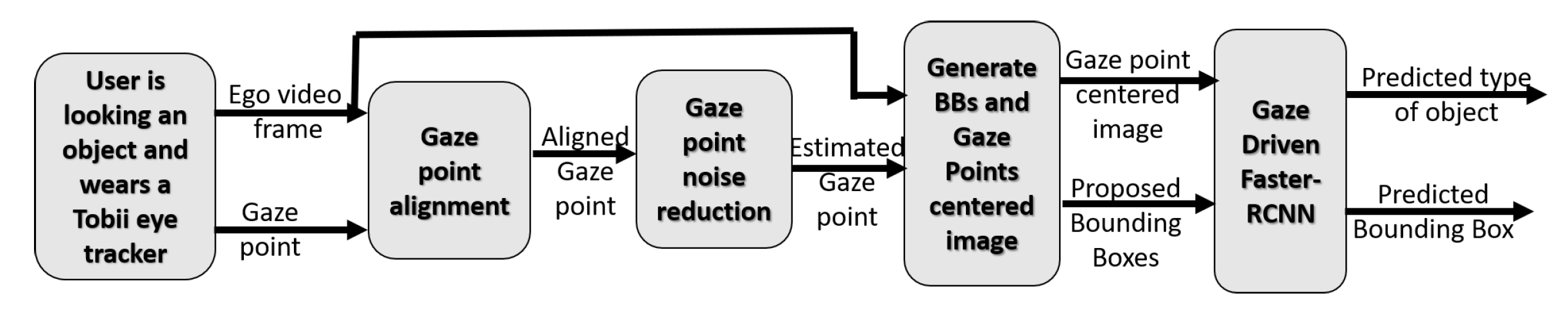
2.1. System Overview
2.2. Gaze Point Alignment
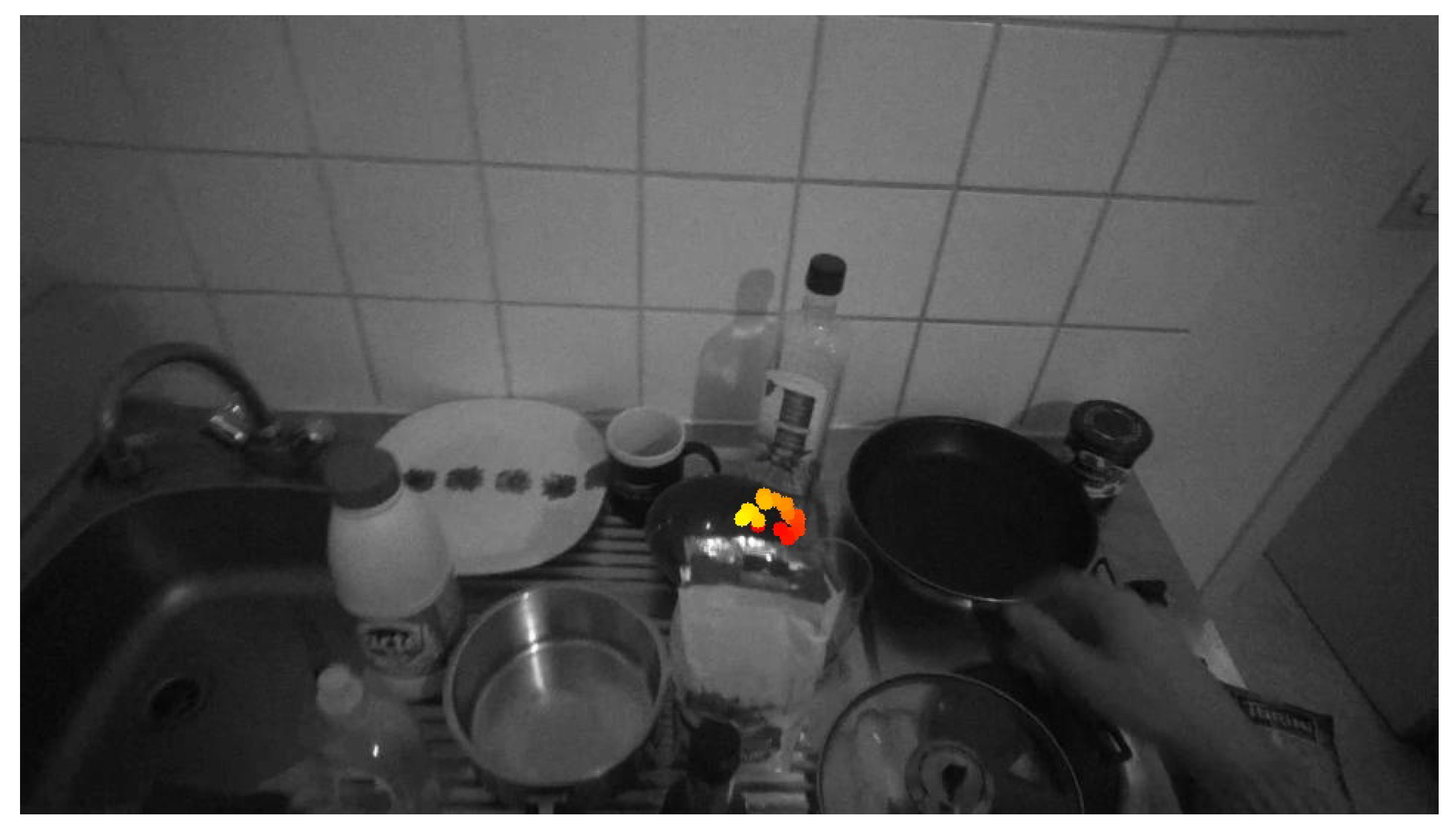
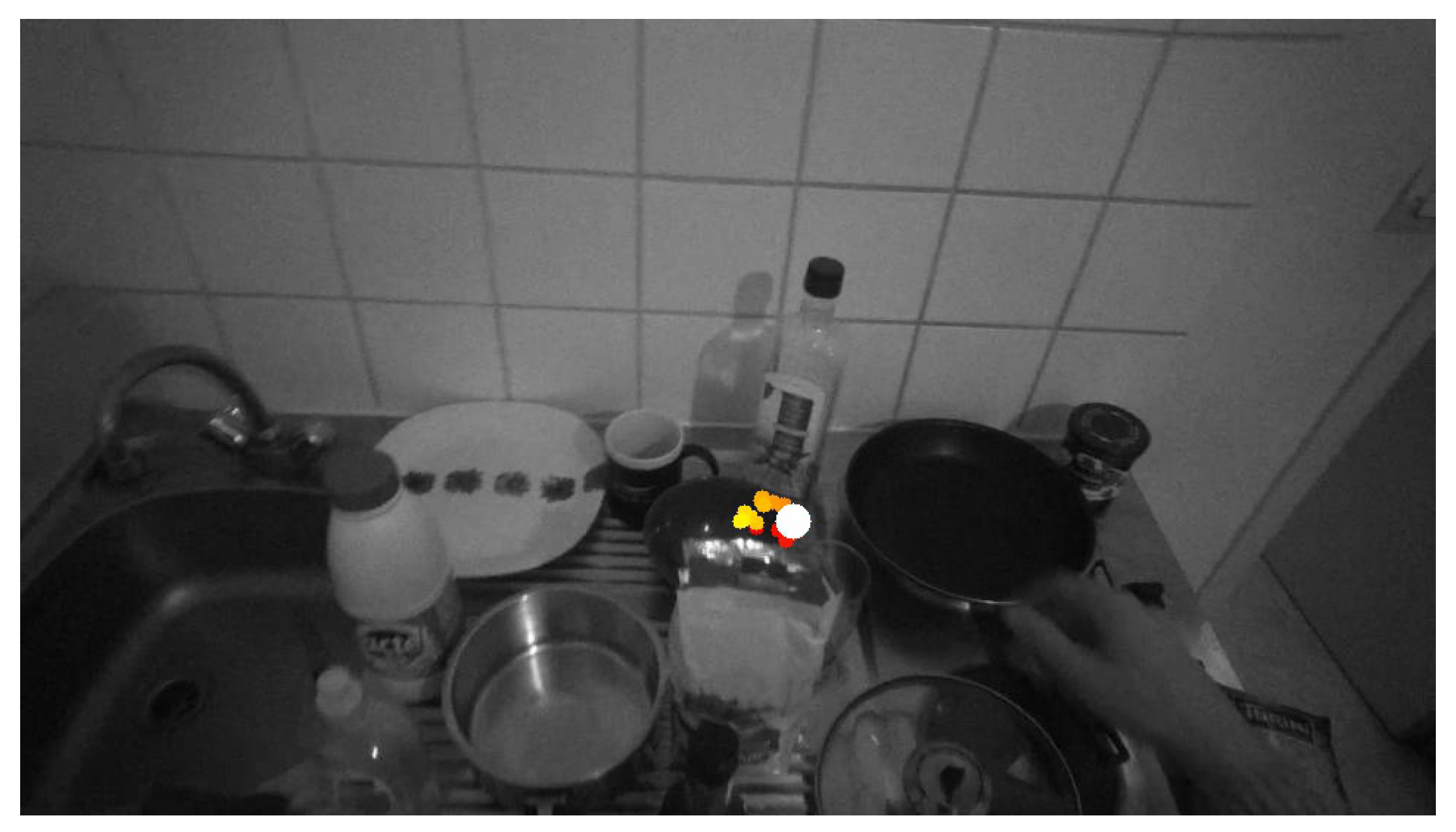
2.3. Noise Reduction
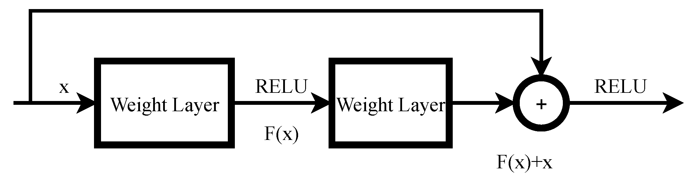
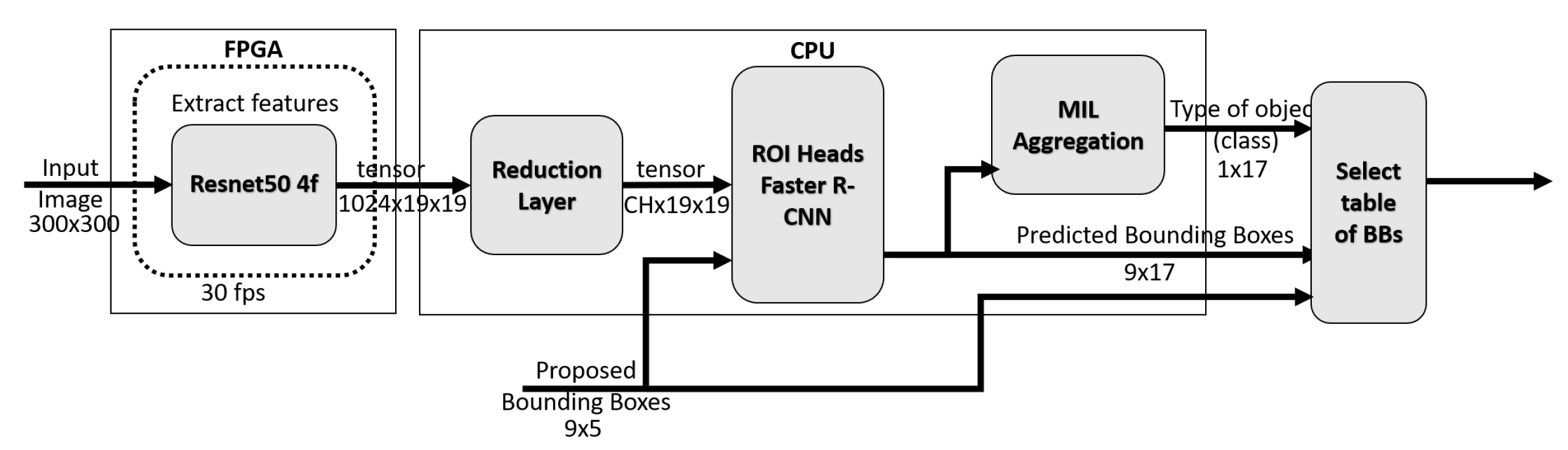
2.4. Gaze-Driven Object Recognition CNN
3. System Hybridization
4. Results
4.1. Dataset
4.2. Geometric Alignment Measurements
4.3. Kernel Density Estimation
4.4. Bounding Box Generation Time Measurements
4.5. Gaze-Driven Object-Recognition CNN Time Measurements
4.6. Gaze-Driven Faster RCNN Accuracy
4.7. Time Measurement of the Whole System
5. Conclusions and Perspectives
Author Contributions
Funding
Institutional Review Board Statement
Informed Consent Statement
Data Availability Statement
Conflicts of Interest
Abbreviations
| BB | bounding box |
| Resnet | deep residual networks |
| CNN | convolutional neural network |
| SIFT | scale invariant feature transform |
| KDE | kernel density estimation |
| MIL | multiple instance learning |
| FPGA | field-programmable gate array |
| FPS | frame rate per second |
| FLANN | fast library for approximate nearest neighbors |
| Faster R-CNN | faster regions with CNN |
| KP | keypoints |
| GITW | grasping-in-the-wild dataset |
| DNN | deep neural network |
| EMG | electromyography |
| YOLO | you only look once |
| SSD | single shot detector |
| VGGnet | very deep convolutional networks |
| DSP | digital signal processing |
| MAC | multiply–accumulate |
| MADD | multiply–add |
| RL | reduction layer |
References
- Kanishka Madusanka, D.G.; Gopura, R.A.R.C.; Amarasinghe, Y.W.R.; Mann, G.K.I. Hybrid Vision Based Reach-to-Grasp Task Planning Method for Trans-Humeral Prostheses. IEEE Access 2017, 5, 16149–16161. [Google Scholar] [CrossRef]
- Mick, S.; Segas, E.; Dure, L.; Halgand, C.; Benois-Pineau, J.; Loeb, G.E.; Cattaert, D.; de Rugy, A. Shoulder kinematics plus contextual target information enable control of multiple distal joints of a simulated prosthetic arm and hand. J. Neuroeng. Rehabil. 2021, 18, 3. [Google Scholar] [CrossRef] [PubMed]
- Han, M.; Günay, S.Y.; Schirner, G.; Padır, T.; Erdoğmuş, D. HANDS: A multimodal dataset for modeling toward human grasp intent inference in prosthetic hands. Intell. Serv. Robot. 2020, 13, 179–185. [Google Scholar] [CrossRef] [PubMed]
- González-Díaz, I.; Benois-Pineau, J.; Domenger, J.P.; Cattaert, D.; de Rugy, A. Perceptually-guided deep neural networks for ego-action prediction: Object grasping. Pattern Recognit. 2019, 88, 223–235. [Google Scholar] [CrossRef]
- Fejér, A.; Nagy, Z.; Benois-Pineau, J.; Szolgay, P.; de Rugy, A.; Domenger, J.P. Implementation of Scale Invariant Feature Transform detector on FPGA for low-power wearable devices for prostheses control. Int. J. Circ. Theor. Appl. 2021, 49, 2255–2273. Available online: http://xxx.lanl.gov/abs/https://onlinelibrary.wiley.com/doi/pdf/10.1002/cta.3025 (accessed on 30 December 2021). [CrossRef]
- Hussein, M.T. A review on vision-based control of flexible manipulators. Adv. Robot. 2015, 29, 1575–1585. [Google Scholar] [CrossRef]
- Mick, S.; Lapeyre, M.; Rouanet, P.; Halgand, C.; Benois-Pineau, J.; Paclet, F.; Cattaert, D.; Oudeyer, P.Y.; de Rugy, A. Reachy, a 3D-Printed Human-Like Robotic Arm as a Testbed for Human-Robot Control Strategies. Front. Neurorobotics 2019, 13, 65. [Google Scholar] [CrossRef] [Green Version]
- Scott, S.H. A functional taxonomy of bottom-up sensory feedback processing for motor actions. Trends Neurosci. 2016, 39, 512–526. [Google Scholar] [CrossRef]
- Miall, R.C.; Jackson, J.K. Adaptation to visual feedback delays in manual tracking: Evidence against the Smith Predictor model of human visually guided action. Exp. Brain Res. 2006, 172, 77–84. [Google Scholar] [CrossRef]
- Ren, S.; He, K.; Girshick, R.; Sun, J. Faster R-CNN: Towards Real-Time Object Detection with Region Proposal Networks. IEEE Trans. Pattern Anal. Mach. Intell. 2017, 39, 1137–1149. [Google Scholar] [CrossRef] [Green Version]
- Redmon, J.; Divvala, S.; Girshick, R.; Farhadi, A. You Only Look Once: Unified, Real-Time Object Detection. arXiv 2016, arXiv:1506.02640. [Google Scholar]
- Liu, W.; Anguelov, D.; Erhan, D.; Szegedy, C.; Reed, S.; Fu, C.Y.; Berg, A.C. SSD: Single Shot MultiBox Detector. In European Conference on Computer Vision; Lecture Notes in Computer Science; Springer: Cham, Switzerland, 2016; pp. 21–37. [Google Scholar] [CrossRef] [Green Version]
- He, K.; Zhang, X.; Ren, S.; Sun, J. Deep Residual Learning for Image Recognition. In Proceedings of the 2016 IEEE Conference on Computer Vision and Pattern Recognition (CVPR), Las Vegas, NV, USA, 27–30 June 2016; pp. 770–778. [Google Scholar] [CrossRef] [Green Version]
- Simonyan, K.; Zisserman, A. Very Deep Convolutional Networks for Large-Scale Image Recognition. arXiv 2015, arXiv:1409.1556. [Google Scholar]
- Krizhevsky, A.; Sutskever, I.; Hinton, G.E. ImageNet Classification with Deep Convolutional Neural Networks. Commun. ACM 2017, 60, 84–90. [Google Scholar] [CrossRef]
- Howard, A.G.; Zhu, M.; Chen, B.; Kalenichenko, D.; Wang, W.; Weyand, T.; Andreetto, M.; Adam, H. MobileNets: Efficient Convolutional Neural Networks for Mobile Vision Applications. arXiv 2017, arXiv:1704.04861. [Google Scholar]
- Szegedy, C.; Liu, W.; Jia, Y.; Sermanet, P.; Reed, S.; Anguelov, D.; Erhan, D.; Vanhoucke, V.; Rabinovich, A. Going deeper with convolutions. In Proceedings of the 2015 IEEE Conference on Computer Vision and Pattern Recognition (CVPR), Boston, MA, USA, 7–12 June 2015; pp. 1–9. [Google Scholar] [CrossRef] [Green Version]
- Grasping in the Wild. Available online: https://www.labri.fr/projet/AIV/dossierSiteRoBioVis/GraspingInTheWildV2.htm (accessed on 30 December 2021).
- Huang, J.; Rathod, V.; Sun, C.; Zhu, M.; Korattikara, A.; Fathi, A.; Fischer, I.; Wojna, Z.; Song, Y.; Guadarrama, S.; et al. Speed/accuracy trade-offs for modern convolutional object detectors. arXiv 2017, arXiv:1611.10012. [Google Scholar]
- Redmon, J.; Farhadi, A. YOLO9000: Better, Faster, Stronger. arXiv 2016, arXiv:1612.08242. [Google Scholar]
- Fejér, A.; Nagy, Z.; Benois-Pineau, J.; Szolgay, P.; de Rugy, A.; Domenger, J.P. FPGA-based SIFT implementation for wearable computing. In Proceedings of the 2019 IEEE 22nd International Symposium on Design and Diagnostics of Electronic Circuits Systems (DDECS), Cluj-Napoca, Romania Balkans, 24–26 April 2019; pp. 1–4. [Google Scholar] [CrossRef]
- Fejér, A.; Nagy, Z.; Benois-Pineau, J.; Szolgay, P.; de Rugy, A.; Domenger, J.P. Array computing based system for visual servoing of neuroprosthesis of upper limbs. In Proceedings of the 2021 17th International Workshop on Cellular Nanoscale Networks and their Applications (CNNA), Catania, Italy, 29 September–1 October 2021; pp. 1–5. [Google Scholar] [CrossRef]
- Kathail, V. Xilinx Vitis Unified Software Platform; FPGA ’20; Association for Computing Machinery: New York, NY, USA, 2020; pp. 173–174. [Google Scholar] [CrossRef] [Green Version]
- Moreau, T.; Chen, T.; Vega, L.; Roesch, J.; Yan, E.; Zheng, L.; Fromm, J.; Jiang, Z.; Ceze, L.; Guestrin, C.; et al. A Hardware–Software Blueprint for Flexible Deep Learning Specialization. IEEE Micro 2019, 39, 8–16. [Google Scholar] [CrossRef] [Green Version]
- Pappalardo, A. Xilinx/Brevitas 2021. Available online: https://zenodo.org/record/5779154#.YgNP6fgRVPY (accessed on 30 December 2021). [CrossRef]
- Umuroglu, Y.; Fraser, N.J.; Gambardella, G.; Blott, M.; Leong, P.; Jahre, M.; Vissers, K. FINN: A Framework for Fast, Scalable Binarized Neural Network Inference. In Proceedings of the 2017 ACM/SIGDA International Symposium on Field-Programmable Gate Arrays, Monterey, CA, USA, 22–24 February 2017. [Google Scholar] [CrossRef] [Green Version]
- Lowe, D.G. Distinctive Image Features from Scale-Invariant Keypoints. Int. J. Comput. Vis. 2004, 60, 91–110. [Google Scholar] [CrossRef]
- OpenCV. A FLANN-Based Matcher Tutorial. Available online: https://docs.opencv.org/3.4/d5/d6f/tutorial_feature_flann_matcher.html (accessed on 30 December 2021).
- 2.8. Density Estimation. Available online: https://scikit-learn.org/stable/modules/density.html (accessed on 30 December 2021).
- PyTorch CONV2D. Available online: https://pytorch.org/docs/stable/generated/torch.nn.Conv2d.htmll (accessed on 30 December 2021).
- Girshick, R. Fast R-CNN. arXiv 2015, arXiv:1504.08083. [Google Scholar]
- Amores, J. Multiple instance classification: Review, taxonomy and comparative study. Artif. Intell. 2013, 201, 81–105. [Google Scholar] [CrossRef]
- UG82 ZCU102 Evaluation Board—User Guide. Available online: https://www.xilinx.com/support/documentation/boards_and_kits/zcu102/ug1182-zcu102-eval-bd.pdf (accessed on 30 December 2021).
- Blott, M.; Preußer, T.B.; Fraser, N.J.; Gambardella, G.; O’Brien, K.; Umuroglu, Y.; Leeser, M.; Vissers, K. FINN-R: An End-to-End Deep-Learning Framework for Fast Exploration of Quantized Neural Networks. ACM Trans. Reconfigurable Technol. Syst. 2018, 11, 1–23. [Google Scholar] [CrossRef]
- Xilinx. PG338—Zynq DPU v3.3 IP Product Guide (v3.3). Available online: https://www.xilinx.com/support/documentation/ip_documentation/dpu/v3_3/pg338-dpu.pdf (accessed on 30 December 2021).
- Intel i5 7300HQ. Available online: https://ark.intel.com/content/www/us/en/ark/products/97456/intel-core-i57300hq-processor-6m-cache-up-to-3-50-ghz.html (accessed on 30 December 2021).
- Zynq UltraScale+ MPSoC Data Sheet: Overview. Available online: https://www.xilinx.com/support/documentation/data_sheets/ds891-zynq-ultrascale-plus-overview.pdf (accessed on 30 December 2021).
- Bradski, G. The OpenCV Library. Dr. Dobb’s J. Softw. Tools 2000, 25, 120–123. [Google Scholar]
- Paszke, A.; Gross, S.; Massa, F.; Lerer, A.; Bradbury, J.; Chanan, G.; Killeen, T.; Lin, Z.; Gimelshein, N.; Antiga, L.; et al. PyTorch: An Imperative Style, High-Performance Deep Learning Library. arXiv 2019, arXiv:1912.01703. [Google Scholar]
- UG1431 (v1.4): ZCU102 Evaluation Kit. Available online: https://www.xilinx.com/html_docs/vitis_ai/1_4/ctl1565723644372.html (accessed on 30 December 2021).


| Module | CPU | FPGA |
|---|---|---|
| Gaze-Point Alignment Block | ||
| SIFT Detection [5] | - | X |
| SIFT Matching | X | - |
| Homography estimation | X | - |
| Gaze-point projection | X | - |
| Gaze-Point Noise Reduction Block | ||
| KDE estimation | X | - |
| Module | CPU | FPGA |
|---|---|---|
| Resnet50 | - | X |
| Reduction layer | X | - |
| Faster R-CNN | X | - |
| MIL aggregation | X | - |
| Xilinx ZCU102 ARM CORTEX A53 | |||||
|---|---|---|---|---|---|
| Video File Name | Mask Radius | SIFT KP Extractions (ms) | Matcher (ms) | Homography (ms) | Gaze Projection (ms) |
| BowlPlace1Subject1 | 119 ± 25 | 875.504 ± 12.123 | 23.471 ± 5.203 | 2.200 ± 0.540 | 0.089 ± 0.004 |
| BowlPlace1Subject2 | 106 ± 16 | 875.282 ± 9.504 | 20.036 ± 3.704 | 1.900 ± 0.398 | 0.088 ± 0.001 |
| BowlPlace1Subject3 | 153 ± 50 | 873.072 ± 7.283 | 17.626 ± 3.276 | 2.539 ± 0.621 | 0.089 ± 0.001 |
| BowlPlace1Subject4 | 120 ± 25 | 873.545 ± 9.062 | 22.244 ± 5.938 | 2.160 ± 0.464 | 0.092 ± 0.009 |
| BowlPlace4Subject1 | 158 ± 55 | 855.947 ± 6.583 | 16.011 ± 3.053 | 2.883 ± 1.188 | 0.088 ± 0.001 |
| BowlPlace4Subject2 | 117 ± 24 | 861.933 ± 5.821 | 16.276 ± 2.623 | 1.997 ± 0.449 | 0.089 ± 0.004 |
| BowlPlace4Subject3 | 108 ± 19 | 867.649 ± 8.894 | 15.679 ± 4.620 | 2.136 ± 0.350 | 0.089 ± 0.005 |
| BowlPlace4Subject4 | 147 ± 49 | 857.271 ± 9.468 | 16.762 ± 4.186 | 2.240 ± 0.516 | 0.088 ± 0.001 |
| BowlPlace5Subject1 | 120 ± 33 | 861.481 ± 8.012 | 17.875 ± 2.176 | 2.018 ± 0.505 | 0.088 ± 0.001 |
| BowlPlace5Subject2 | 133 ± 42 | 858.547 ± 6.232 | 17.944 ± 3.024 | 2.354 ± 0.880 | 0.088 ± 0.001 |
| BowlPlace5Subject3 | 126 ± 33 | 859.774 ± 6.384 | 15.742 ± 2.836 | 2.007 ± 0.524 | 0.087 ± 0.001 |
| BowlPlace6Subject1 | 120 ± 25 | 867.344 ± 10.950 | 19.026 ± 3.862 | 1.965 ± 0.306 | 0.088 ± 0.001 |
| BowlPlace6Subject2 | 129 ± 35 | 862.750 ± 9.731 | 19.737 ± 4.973 | 3.681 ± 3.456 | 0.090 ± 0.008 |
| BowlPlace6Subject3 | 127 ± 31 | 864.429 ± 6.931 | 17.555 ± 3.806 | 2.588 ± 0.823 | 0.087 ± 0.001 |
| BowlPlace6Subject4 | 112 ± 22 | 867.962 ± 9.579 | 17.368 ± 4.725 | 2.710 ± 0.649 | 0.089 ± 0.004 |
| Intel i5 7300HQ | |||||
| Video File Name | Number of Extracted KP | SIFT KP Extractions (ms) | Matcher (ms) | Homography (ms) | Gaze Projection (ms) |
| BowlPlace1Subject1 | 151 ± 67 | 74.205 ± 5.611 | 3.891 ± 0.853 | 0.259 ± 0.051 | 0.015 ± |
| BowlPlace1Subject2 | 156 ± 37 | 75.062 ± 5.640 | 3.304 ± 0.579 | 0.228 ± 0.040 | 0.014 ± |
| BowlPlace1Subject3 | 86 ± 50 | 72.217 ± 2.572 | 3.011 ± 0.476 | 0.282 ± 0.055 | 0.014 ± |
| BowlPlace1Subject4 | 138 ± 69 | 72.979 ± 2.853 | 3.717 ± 0.940 | 0.252 ± 0.044 | 0.015 ± 0.002 |
| BowlPlace4Subject1 | 94 ± 50 | 70.068 ± 2.405 | 2.747 ± 0.565 | 0.313 ± 0.113 | 0.014 ± |
| BowlPlace4Subject2 | 121 ± 28 | 72.280 ± 3.538 | 2.778 ± 0.407 | 0.233 ± 0.040 | 0.015 ± |
| BowlPlace4Subject3 | 126 ± 39 | 73.402 ± 3.406 | 2.678 ± 0.728 | 0.256 ± 0.047 | 0.014 ± |
| BowlPlace4Subject4 | 95 ± 50 | 70.394 ± 2.349 | 2.872 ± 0.695 | 0.259 ± 0.051 | 0.014 ± |
| BowlPlace5Subject1 | 129 ± 39 | 71.990 ± 2.691 | 3.027 ± 0.369 | 0.244 ± 0.050 | 0.015 ± |
| BowlPlace5Subject2 | 120 ± 56 | 71.587 ± 2.526 | 3.077 ± 0.573 | 0.272 ± 0.087 | 0.014 ± |
| BowlPlace5Subject3 | 108 ± 36 | 71.359 ± 2.500 | 2.684 ± 0.448 | 0.234 ± 0.049 | 0.015 ± 0.001 |
| BowlPlace6Subject1 | 132 ± 48 | 72.150 ± 2.891 | 3.213 ± 0.645 | 0.237 ± 0.031 | 0.015 ± |
| BowlPlace6Subject2 | 129 ± 59 | 71.790 ± 3.934 | 3.348 ± 0.823 | 0.390 ± 0.316 | 0.015 ± |
| BowlPlace6Subject3 | 114 ± 47 | 72.042 ± 2.883 | 2.976 ± 0.617 | 0.287 ± 0.076 | 0.015 ± 0.001 |
| BowlPlace6Subject4 | 138 ± 44 | 74.585 ± 4.431 | 3.089 ± 0.849 | 0.303 ± 0.075 | 0.015 ± |
| Xilinx ZCU102 ARM CORTEX A53 | Intel i5 7300HQ | ||||
|---|---|---|---|---|---|
| Video File Name | Gaze Points | Time (ms) | Max Time (ms) | Time (ms) | Max Time (ms) |
| Bowl | 22 ± 8 | 49.27 ± 82.83 | 307.34 | 4.94 ± 7.68 | 27.90 |
| CanOfCocaCola | 26 ± 11 | 75.54 ± 95.89 | 395.08 | 7.46 ± 8.80 | 36.70 |
| FryingPan | 24 ± 9 | 59.09 ± 50.06 | 206.76 | 5.86 ± 4.51 | 18.98 |
| Glass | 29 ± 10 | 148.22 ± 265.60 | 943.19 | 14.89 ± 26.23 | 92.21 |
| Jam | 27 ± 12 | 132.75 ± 319.01 | 1365.65 | 13.34 ± 31.39 | 134.68 |
| Lid | 29 ± 16 | 247.21 ± 718.32 | 3835.30 | 23.92 ± 70.97 | 379.64 |
| MilkBottle | 28 ± 10 | 114.95 ± 148.60 | 647.86 | 11.20 ± 13.99 | 61.92 |
| Mug | 28 ± 11 | 109.88 ± 218.40 | 1087.39 | 11.03 ± 21.26 | 106.63 |
| OilBottle | 30 ± 12 | 235.15 ± 477.79 | 2117.26 | 22.86 ± 46.23 | 205.83 |
| Plate | 32 ± 14 | 203.39 ± 406.91 | 1837.70 | 19.59 ± 39.46 | 178.97 |
| Rice | 29 ± 13 | 90.34 ± 95.16 | 372.93 | 8.64 ± 8.92 | 35.80 |
| SaucePan | 25 ± 12 | 139.07 ± 261.08 | 1286.11 | 13.68 ± 25.82 | 126.92 |
| Sponge | 24 ± 10 | 50.05 ± 49.79 | 207.89 | 5.10 ± 4.76 | 20.46 |
| Sugar | 27 ± 14 | 146.60 ± 271.58 | 1165.44 | 14.46 ± 26.70 | 117.57 |
| VinegarBottle | 28 ± 13 | 122.32 ± 178.37 | 683.56 | 12.23 ± 17.71 | 70.01 |
| WashLiquid | 28 ± 12 | 102.93 ± 183.02 | 880.47 | 10.42 ± 18.45 | 89.25 |
| Number of Channel | Backbone (ms) | Reduction Layer (ms) | ROI Heads (ms) | Aggregation (ms) |
|---|---|---|---|---|
| 32 | 90.000 ± 0.250 | 0.336 ± | 1.107 ± | 0.137 ± |
| 64 | 97.307 ± 1.613 | 0.531 ± 0.002 | 2.262 ± 0.004 | 0.138 ± |
| 96 | 87.441 ± 0.508 | 0.557 ± 0.003 | 2.956 ± 0.003 | 0.241 ± |
| 128 | 89.952 ± 2.568 | 0.646 ± 0.001 | 3.356 ± 0.001 | 0.142 ± |
| 256 | 85.287 ± 0.375 | 0.908 ± | 6.592 ± 0.002 | 0.150 ± |
| 512 | 94.505 ± 2.100 | 2.485 ± 0.002 | 12.276 ± 0.002 | 0.159 ± |
| 1024 | 95.515 ± 7.285 | 3.204 ± 0.007 | 23.718 ± 0.010 | 0.164 ± |
| Number of Channel | Backbone (ms) | Reduction Layer (ms) | ROI Heads (ms) | Aggregation (ms) |
|---|---|---|---|---|
| 32 | 1863.300 ± 11.433 | 6.949 ± 0.001 | 13.843 ± 0.002 | 0.643 ± 0.001 |
| 64 | 1768.616 ± 15.615 | 8.156 ± 0.001 | 21.859 ± 0.006 | 0.708 ± |
| 96 | 1787.737 ± 15.903 | 10.178 ± 0.001 | 30.705 ± 0.001 | 0.758 ± |
| 128 | 1800.327 ± 17.915 | 12.140 ± 0.001 | 39.371 ± 0.002 | 0.727 ± |
| 256 | 1797.798 ± 16.372 | 22.061 ± 0.011 | 73.750 ± 0.002 | 0.714 ± |
| 512 | 1733.458 ± 14.429 | 33.723 ± 0.001 | 142.231 ± 0.001 | 0.752 ± |
| 1024 | 1761.748 ± 16.305 | 63.319 ± 0.001 | 285.121 ± 0.002 | 0.714 ± |
| Number of Channel | 32 | 64 | 96 | 128 | 256 | 512 | 1024 |
|---|---|---|---|---|---|---|---|
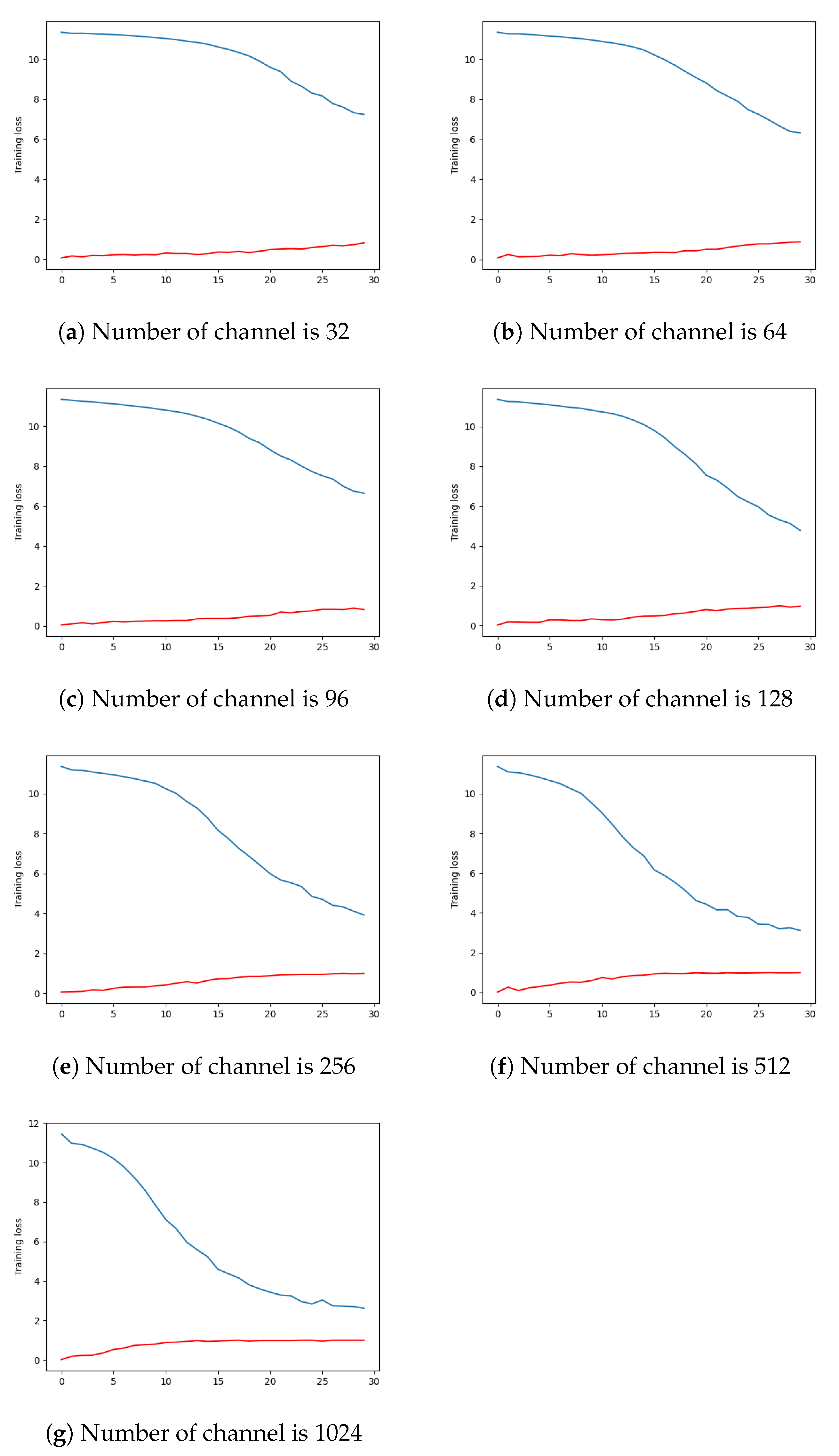
| avg loss on training set | 7.235 | 6.318 | 6.642 | 4.778 | 3.920 | 3.115 | 2.623 |
| avg acc on trainig set | 0.815 | 0.877 | 0.827 | 0.963 | 0.988 | 1.000 | 1.000 |
| avg acc on test set | 0.793 ± 0.261 | 0.926 ± 0.120 | 0.853 ± 0.161 | 0.952 ± 0.083 | 1.000 | 1.000 | 1.000 |
| avg ap on test set | 0.978 ± 0.043 | 0.985 ± 0.030 | 0.964 ± 0.041 | 0.995 ± 0.012 | 1.000 | 1.000 | 1.000 |
| Name | Gaze-Driven, Object-Recognition CNN | SSD Mobilnet V2 | YOLO V3 |
|---|---|---|---|
| Dataset | GITW | COCO | VOC |
| Framework | Pytorch | Tensorflow | Tensorflow |
| Input size | 300 × 300 | 300 × 300 | 416 × 416 |
| Running device | ZCU 102 + ARM A53 | ZCU 102 | ZCU 102 |
| FPS | 12.64 | 78.8 | 13.2 |
| Computational Time (ms) | |||
|---|---|---|---|
| Module Name | Intel i5 7300HQ CPU | ARM A53 | FPGA + ARM A53 |
| SIFT [27] | 72.407 ± 3.349 | 865.499 ± 8.437 | 7.407 [5] |
| FLANN matcher | 3.094 ± 0.638 | 18.223 ± 3.867 | 18.223 ± 3.867 |
| Homography estimation | 0.270 ± 0.075 | 2.359 ± 0.778 | 2.359 ± 0.778 |
| Gaze point projection | 0.015 ± | 0.089 ± 0.003 | 0.089 ± 0.003 |
| KDE estimation | 12.477 ± 23.306 | 126.672 ± 238.900 | 126.672 ± 238.900 |
| Bounding Box generation | 0.424 ± 0.020 | 2.659 ± 0.027 | 2.659 ± 0.027 |
| Resnet50 [13] | 89.952 ± 2.568 | 1800.327 ± 17.915 | 26.860 |
| Reduction Layer | 0.645 ± 0.001 | 12.140 ± 0.001 | 12.140 ± 0.001 |
| Faster R-CNN [10] | 3.356 ± 0.001 | 39.371 ± 0.002 | 39.371 ± 0.002 |
| MIL Aggregation | 0.142 ± | 0.727 ± | 0.727 ± |
| Total time (ms) | 182.782 ± 29.957 | 2868.066 ± 269.930 | 236.507 ± 243.578 |
Publisher’s Note: MDPI stays neutral with regard to jurisdictional claims in published maps and institutional affiliations. |
© 2022 by the authors. Licensee MDPI, Basel, Switzerland. This article is an open access article distributed under the terms and conditions of the Creative Commons Attribution (CC BY) license (https://creativecommons.org/licenses/by/4.0/).
Share and Cite
Fejér, A.; Nagy, Z.; Benois-Pineau, J.; Szolgay, P.; de Rugy, A.; Domenger, J.-P. Hybrid FPGA–CPU-Based Architecture for Object Recognition in Visual Servoing of Arm Prosthesis. J. Imaging 2022, 8, 44. https://doi.org/10.3390/jimaging8020044
Fejér A, Nagy Z, Benois-Pineau J, Szolgay P, de Rugy A, Domenger J-P. Hybrid FPGA–CPU-Based Architecture for Object Recognition in Visual Servoing of Arm Prosthesis. Journal of Imaging. 2022; 8(2):44. https://doi.org/10.3390/jimaging8020044
Chicago/Turabian StyleFejér, Attila, Zoltán Nagy, Jenny Benois-Pineau, Péter Szolgay, Aymar de Rugy, and Jean-Philippe Domenger. 2022. "Hybrid FPGA–CPU-Based Architecture for Object Recognition in Visual Servoing of Arm Prosthesis" Journal of Imaging 8, no. 2: 44. https://doi.org/10.3390/jimaging8020044