Review

The Flows of Nature to People, and of People to Nature: Applying Movement Concepts to Ecosystem Services

by
Rachel Dolan
1,*,
James M. Bullock
2,
Julia P. G. Jones
1,
Ioannis N. Athanasiadis
3,
Javier Martinez-Lopez
4 and
Simon Willcock
1,5
1
School of Natural Sciences, Bangor University, Bangor LL57 2DG, UK
2
NERC Centre for Ecology and Hydrology, Wallingford OX10 8BB, UK
3
Wageningen University and Research, 6708 PB Wageningen, The Netherlands
4
Consejo Superior de Investigaciones Científicas-Centro de Edafología y Biología Aplicada del Segura (CEBAS-CSIC), E-30100 Murcia, Spain
5
Rothamsted Research, Harpenden AL5 2JQ, UK
*
Author to whom correspondence should be addressed.
Land 2021, 10(6), 576; https://doi.org/10.3390/land10060576
Submission received: 27 April 2021 / Revised: 21 May 2021 / Accepted: 25 May 2021 / Published: 29 May 2021
(This article belongs to the Special Issue Exploring the Relationships between Land Use and Ecosystem Services)

Abstract

:
To date, the provision of ecosystem services has largely been estimated based on spatial patterns of land cover alone, using benefit transfer analysis. Although it is increasingly being recognised that the distribution of the human population affects whether a potential service translates into a realised service, this misses key steps in the process and assumes that everyone accesses ecosystem services in the same way. Here we describe a conceptual approach to ecosystem services in terms of movement and flows. We highlight that ecosystem service flows can be broken down into ‘nature to people’ (the movement of nature towards beneficiaries) and ‘people to nature’ (the movement of beneficiaries towards nature). The former has been relatively well described. Here, we explore the latter by reviewing research on human migration, animal foraging and landscape connectivity. We assess if and how existing theories might be useful in describing how people seek out ecosystem services. We consider some of the ways in which flows of people to nature can be measured. Such measurements may reveal which movement theories best represent how people seek out and access ecosystem services. Overall, our review aims to improve the future modelling of ecosystem services by more explicitly considering how people access potential services and therefore realise them.

Graphical Abstract

1. Introduction

Many initial assessments of ecosystem services (ESs; nature’s contribution to people [1]) were based on land cover; i.e., whether an area is woodland, grassland, urban, etc. [2,3]. For example, in a highly influential paper, Costanza et al. [4] estimated the value of global ESs to be approximately USD 33 trillion a year using economic valuations based on land cover. This method consists of matching an ecosystem type with the potential ESs they provide in a lookup table (reviewed by [5]), and it has been widely used. Despite the fact that ESs are an inherently socio-ecological concept [6], the land cover approach considers only ecological variables and does not factor in the social variables. Although this approach may give an estimate of potential ESs [7] or the capacity of an ecosystem to supply a service [8] (e.g., biophysical supply of timber), it does not account for demand or how people might access the service, which is largely unknown [9].
Alternative approaches to lookup tables or ES matrices for assessing ESs include ES modelling (e.g., InVEST), monetary techniques and socio-cultural methods [10]. Monetary techniques estimate the economic value of services, for example using the travel cost method to reveal preferences [11]. Socio-cultural methods seek to understand preferences or social values for ES, for example by asking people to rank the benefits they gain from a space [12]. These methods still do not necessarily account for how people might access and realise the service.
To move beyond assessing potential ESs to assessing realised ESs, human population data can be used to estimate demand for ESs [13,14,15]. Demand for ESs may be considered at local, regional and global scales [16]. In some situations, considering only the local population is appropriate when assessing demand for ES. For example, where fuel is gathered from a woodland by people travelling on foot, then demand can be estimated by using local population density data [15]. However, the demand may also come from beyond the local area. For example, firewood may be collected and transported to another region of the same country or internationally to be sold [17]. In such situations, ecosystems may be ‘telecoupled’ to distant populations [18,19] and so local populations are not always a useful indicator of demand [20]. Indeed, this example illustrates that demand for an ES may be manifested over more than one spatial scale. Considering demand in any way is a marked improvement on merely estimating theoretical supply using land cover [21,22]. However, estimates of demand often do not consider how people access a service or how the service might reach them, i.e., the spatio-temporal process by which the service is realised [23]. For example, although every human on Earth benefits from carbon sequestration via the omni-directional dispersal of benefits throughout the atmosphere [24], other benefits are more localised (e.g., access to a local viewpoint [25]).
ES flow refers to the whole process of a potential ecosystem service becoming realised [26], and requires an understanding of how people access the benefits of ecosystem services [16]. To better understand ES flows, they can be broken down into two processes, which here we term ‘nature to people’ and ‘people to nature’ (based on a previously developed framework; Figure 1 [27,28]). ‘Nature to people’ (N2P) is the movement of a natural good towards the point where the good is used by beneficiaries (i.e., a flow of nature to beneficiaries (the end-users)), and thus becomes an ES [29]. In order for a natural good to become an ES, some human input is needed, and so a ‘transactor’ (Figure 1) is needed to translate the good into a service [27,28,29,30]. The transactor is the point at which a service becomes realised. For example, a river will flow down a mountain (N2P) and people will go to the river (P2N) to fish. The point at which they catch the fish is the transactor.
‘People to nature’ (P2N) is the movement of beneficiaries to a transactor in the search for an ecosystem service (i.e., a flow of beneficiaries to nature). For example, a view-point within a National Park is a possible transactor; from this point beneficiaries access views of the landscape. Alternatively, when considering people going to a forest to collect firewood, the point in the forest/landscape where the wood is collected would be the transactor [31]. In some cases, people going to nature might be the realisation of the service itself; for example, going for a bike ride through a woodland (Figure 1). Different mechanisms for N2P and P2N are summarised in Table 1, and a series of each might be combined in order to encompass the overall ES flow (e.g., as part of a value chain [27,28]). There is a wealth of literature on N2P both within the ES literature and in other areas of research, for example, the global agri-food system [32] and the global trade of fish from fisheries [33,34]. However, P2N has been much less explored in the ES literature. The first step in filling this knowledge gap is to understand better how ES beneficiaries seek out and access ES—this is the aim of this paper.
ES flows are known to vary across different socioeconomic groups, as people vary in their preferences, as well as in the options available to them. For example, Cumming et al. [35] hypothesised that residents in rural areas may be more directly connected to local ecosystems, whereas those in urban areas rely more heavily on distant ecosystems. However, this hypothesis does not account for the varied experiences of individuals living within such systems. There are inevitable differences in P2N depending on people’s wealth and residential location. For example, there can be a larger cost implication for urban people accessing natural spaces [36,37], although wealthier individuals/families are more likely to have access to private or public green space [38]. By contrast, many urban residents have easier access to shops than rural residents (P2N), where provisional ES can be obtained indirectly via value chains going from producers to shops (N2P) [39]. Similarly, a number of studies have suggested gendered differences in the perception and use of urban green space, for example, in terms of the activities carried out [40], reported benefits [41] and fears about personal safety [42].
It is not the aim of this paper to describe differences among individuals of differing socio-economic groups in terms of ES access in detail, as this has been explored elsewhere (for example, [43] reviews ESs through a gendered lens). Instead, in this conceptual paper, we disaggregate the flow of ES into N2P and P2N and seek to understand the processes by which beneficiaries seek out ESs—the movement of people to nature (P2N). We focus on large-scale, replicable theories, presenting possible approaches by which maps or models of potential ES supply can be supplemented to capture realised ES (i.e., including demand and access). We bring together insights from disciplines that might help understand how people move towards ES, by exploring the potential application of models from human migration, optimal foraging and landscape connectivity. We then present an introduction to some of the data currently available to researchers that could represent ES flows.
As we show in Table 1 and Figure 1, both N2P and P2N can be applied for different types of ES. For a provisioning service such as a food crop, N2P might be the movement of the product through a value chain until it reaches a shop or market. An example of the P2N part of the flow would be an individual going to the point where they can purchase the item. For a regulating service such as flood prevention, N2P is not relevant as such, but people who live in the area that does not flood benefit from this service. Individuals may move specifically to this area to benefit from the low flood risk—an example of P2N. For a cultural service, N2P may occur through line of sight, for example, through enjoying views of mountains from one’s home. Alternatively, people may travel specifically to spend time in the mountains, which would be classified as P2N.

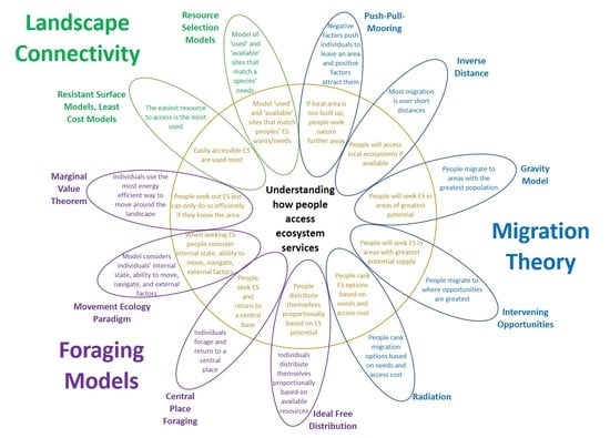
2. Applying Existing Theories of Movement to ‘People to Nature’

2.1. Migration Theory Applied to ‘People to Nature’

P2N could be explored using migration models (Table 2). Noting that migration has a range of definitions across different disciplines, migration can be defined as “the movement of a person or a group of persons, either across an international border…, or within a state…, encompassing any kind of movement of people, whatever its length, composition and causes ” [51]. Thus, migration can be used to describe movement, from short journeys to complete relocation of someone’s life, e.g., [52]. In terms of ES, this could be applied to people making trips to access services such as recreation in their local area (i.e., where their place of residence does not change but they are still moving across the landscape) [53]. It could also be applied to people making longer trips to access ES, for example several nights away camping [54]. It could also be applied to people moving house and basing their choice of location on the ES they can access there [52].
The push-pull-mooring (PPM) model of migration states that decisions to migrate are affected by three different groups of factors [55]. As discussed above, migration sometimes means to relocate one’s place of residence. In this case, push factors ‘push’ people away from one area, for example, a lack of jobs, violence, pollution and poor housing. Pull factors ‘pull’ people towards a different area, such as more job opportunities, better housing and better education opportunities. Mooring factors are influences that hinder the decision to migrate or the process of migrating, for example, financial cost, distance and family considerations. The push-pull-mooring model can also be applied to short-term migration (e.g., for accessing recreation opportunities). For example, a pull factor stated by visitors to parks and protected areas in Portugal was that the parks provided a space to do sports and outdoor activities [56]. Children can be a mooring factor when deciding where to go [57].
As well as migration itself, the PPM is used to understand consumer choices and ‘switching behaviour’ between one service provider and another, such as social media platforms [58] and airline companies [59]. In these cases, push factors include high price, inconvenience, poor-quality service and a lack of trust in the company. A more attractive alternative that offers solutions to these problems pulls people away from their original service provider. Mooring factors include the financial cost and effort of switching and social factors [59]. As this theory is useful in understanding how people choose between one economic/IT service and another, the same theory might shed light on how people choose between two different ways/locations for accessing ESs.
The inverse distance model [36] is based on the idea that distance represents some kind of friction or cost, so that people will access opportunities closer to their starting point. The further they go, the greater the cost in terms of time and money. An increase in travel cost has been shown to have a negative effect on people’s willingness to make a journey [57,60]. Increases in the cost to access a location both in terms of time and money might be linear or the increases might be proportional jumps, such as having to switch transport modes or stay overnight because the intended location is so far away [37]. These proportional jumps might represent ‘cut-off points’ where people are no longer able to access a service or area because it is too expensive for them.
The inverse distance model is used in health care to explore how many people can access services [54]. In health care, access can be considered based on how many people can access services within a specified distance or time limit from where they live, and on the ratio of services to the population [61]. This approach considers the concept of ‘geographical access’, i.e., literally how far away a resource is, and the effective or perceived access, which consider other factors such as financial, social and cultural factors [54]. These concepts could be applied to accessing ESs too. A recreation opportunity could be close by but may be expensive to access, thus rendering it effectively inaccessible for some groups. People may make longer journeys for longer lasting and more rewarding activities. The longer stay or better experience balances the additional cost of travelling further. For example, overnight visitors to National Parks in Germany travelled 3.5 times the distance of non-local day visitors [37]. The parks that received the most overnight visitors were those in harder-to-access locations in the mountains [37]. As a further example, households in Malawi were found to have a greater reliance on forest products to supplement their income the closer they lived to a forest. The further away from the forest they lived, the less rewarding the products were for the cost to obtain them [62].
The gravity model is one of the longest standing in migration literature and comprises the idea that areas of higher ‘mass’ attract more people [36]. This higher mass can be considered in terms of attractiveness or some other factor that pulls people in. Distance is also a factor; if two areas have equal ‘mass’, the one that is further away will be less attractive, an effect known as distance decay. When considering ESs, areas of greater ES potential (such as National Parks) might attract more visitors [37]. These areas attract high numbers of visitors because they are widely acknowledged to provide varied recreational, cultural and heritage opportunities [63]. Similarly, famous tourist attractions draw in more visitors [64]. The significance of areas (the mass) may be further increased through social media, with people choosing locations based on what they have seen online and what they can then share themselves [65]. Alternatively, an area that is very rich in a desired resource such as firewood or a food item will attract more people [66].
The gravity model might be criticised in terms of the validity of using population size as a factor attracting people to the area. It also does not factor in transport networks or costs and does not consider the difference between individuals migrating, treating them as a homogenous group.
Stouffer’s law of intervening opportunities considers the opportunities available at a destination [67]. Migration is proportional to the opportunities at the destination and inversely proportional to those that lie between the starting point and the destination. When considering ESs, areas that provide multiple services are likely to attract lots of visitors. For example, National Parks facilitate different recreational pursuits, and they provide a place to see wildlife, to learn about culture and history, as well as an aesthetically pleasing place in which to be. However, if there was a site nearer to an individual’s starting point that provided some of these opportunities, they might be more inclined to go there, as there is likely less of a cost to access it even if the site is of lower quality. Similarly, when foraging for wild food products, there might be a very rich site further from an individuals’ starting point, but they may choose a poorer site closer to home.
The radiation model [68] builds on the law of intervening opportunities and hypothesises that when making a decision about where to go, people go through two steps. First, they assign all opportunities that they know of a ‘fitness score’ based on how closely they match the experience that they want. Second, they rank the opportunities based on how far they are from their starting point. They choose the closest one that matches the experience they want. For example, people search for jobs in their field and rank them based on how closely the job matches what they want to do and how good the pay is. Then, they rank the jobs based on how far away they are from their home. They choose the closest job that best matches their requirements. The fewer opportunities there are, the further they will have to travel. Marques et al. [69] explored visitors’ motivations for visiting protected areas in Portugal. They identified multiple subgroups of visitors. One group’s priority was to attend local sports or cultural events. Another group’s priority was to see the landscape and the wildlife. The sports group traveled a shorter distance than the cultural group to access protected areas. The cultural group had to go, and were happy to go, further to see a variety of species and habitats. Thus, the visitors had ranked all possible protected areas they could access based on whether it would meet the experience they wanted, then on how far away these areas were, and then decided how far they were willing to go to gain the experience. As such, the movement of these visitors may be well described by the radiation model.

2.2. Animal Foraging Theory Applied to ‘People to Nature’

Behavioural ecology models may be useful in considering ES flows, particularly through models relating to foraging (the search for wild food resources [70], Table 3). Behavioural ecology considers the evolutionary basis for behaviour, i.e., how a behaviour contributes to overall fitness [70]. The process affects fitness because the search for resources expends energy, and accrues other costs such as risk to life, so it is a trade-off between resources gained and the cost to access them. Foraging has been explored using economic models, specifically the ‘optimal model’, which represents an animal foraging to obtain the maximum reward for minimal effort [71]. P2N can be considered as humans ‘foraging’ for nature as people search the environment for resources and opportunities.
Foraging models often assume that knowledge of opportunities is based on what is learnt from the environment and from previous experience. In addition, animals may also use social information when foraging (e.g., in birds [72] and bats [73]). When considering how people access ES, we need to consider that they will use also social information learnt directly from their network and also from social media [74]. People have the ability to research and learn about areas before they go there.
The marginal value theorem assumes that animals will use the most energy efficient method to forage [75]. It assumes that animals exist in an environment with patches of resources separated by areas with no resources, so they must expend energy moving from one to the other. They have to balance how long they spend at a patch with travelling between patches and how much they will gain from each patch. Resources will diminish the longer they stay at a patch. Cowie [76] investigated whether the behaviour of foraging great tits (Parus major) can be predicted by the marginal value theorem [76]. In his experiment, great tits were allowed to forage in areas that differed in terms of the distance between resource patches and patch richness. In keeping with marginal value theorem, the birds spent longer at each patch when the patches were further apart and when they had greater resources. Birds left patches when resource levels fell below the average for the whole area, which is a more efficient way to forage, with a higher reward compared to foraging randomly [77].
There are examples of humans following the marginal value theorem. Wolfe [78] carried out a virtual raspberry picking experiment and found that people’s behaviour was in keeping with marginal value theorem. They would move on from one bush to the next when the number of berries fell below the average for the whole area, and they would stay longer when it took longer to travel from one bush to the next. Their behaviour departed from the marginal value theorem if patches varied in quality, in which case people would stay at the same bush when it would have been more beneficial to move on. When considering ESs, the resource may not necessarily run out but service quality may become degraded after repeated access; for example, the habitat may become degraded, which reduces the quality of the experience [79].
The marginal value theorem assumes ‘perfect knowledge’ of the environment; it does not consider individuals exploring an unfamiliar area, where they might not know how rich the resources are so will spend more time familiarising themselves [80]. It also does not consider other factors affecting an individual, such as their physiological state or other individuals around them, such as their offspring, potential mates or predators that might affect their behaviour or compete with them [80]. Therefore, the marginal value theorem can be helpful in exploring how people access ESs, especially in a familiar environment, but it does not consider the whole picture.
Central place foraging theory comprises the idea that an individual will forage at a particular patch and then must return to a central place. The further they have to go from their central point, the more costly the journey, so the value of the resource they are seeking has to increase to match this. For example, beavers bring back larger saplings when they travel further from the lodge [81]. Adapting this theory for P2N, we might consider the central place as a person’s residence or home area, depending on the scale of the study [82]. The theory predicts that the further away an individual travels from their central point, the longer they will stay there. Central place foraging has been observed in the case of artisanal fishers setting up ‘moored fish aggregating devices’ in Dominica [83]. As a cultural ES example, visitors to the Atlantic Coast in the United States were found to stay longer the further away they had come from [84]. However, costs, the characteristics of the people travelling, transport options and time constraints are also likely to factor into these decisions [85].
The ideal free distribution (IFD) also considers the way animals distribute themselves among patches of resources. The IFD considers the effect of other individuals, assuming that animals are free to move between different patches and that each patch has a value depending on how resource-rich it is and how many other individuals are also on this patch. Individuals are aware of the value of all available patches and are competitively equal, and increasing the number of individuals reduces the value of the patch [86]. Distribution should be proportional to the resources available, so if the availability of resources changes, for example, due to more individuals arriving and increasing competition, the distribution of individuals should change to rebalance the distribution. For example, free-ranging cattle in Norway were observed to graze in areas providing lower-quality grazing when the density of cattle was higher. Individuals moved away from the areas with more palatable grazing as competition increased [87]. People have also been observed to follow the IFD. Moritz et al. [88] observed mobile pasturalists to follow IFD in common-pool grazing areas in Cameroon. Disma et al. [89] observed children selling bottles of water to drivers at a crossroads in Istanbul, Turkey. In keeping with IFD, as the number of vehicles in each lane (the number of foraging opportunities) changed, the children redistributed themselves [89].
The IFD would predict high levels of ES use in areas that provide high levels of ESs. For example, protected areas attract a lot of people seeking cultural services compared to areas that are less rich in wildlife and opportunities [63]. Similarly, Willcock et al. [66] found that people in Tanzania are more likely to live in areas of high biodiversity resources that allow them to access more ESs [66]. IFD would also predict that the higher the use of ES hotspots, the more people will spread out to areas that provide fewer opportunities. Even though there are fewer opportunities to access ESs there, there may be a greater chance to do so because there are less people competing for them. For example, bird watchers can put off spending time at very popular sites because due to the amount of people there, they may actually be less likely to see species of interest [90]. Like the marginal value theorem, the IFD does not consider individuals who are unfamiliar with an area, nor does it consider other social or internal factors that might influence their decisions [80].
The movement ecology paradigm [91] considers a wide range of factors: the internal state of the individual (why they move), how they move from one site to another, their ability to navigate and external factors that might affect them. For example, a vulture is foraging because it needs food (internal state) but it also has to conserve energy levels; therefore, as the time since it has last eaten increases, it changes its foraging strategy to save energy by using uplifts as much as possible and avoiding flapping and take-offs/landing, which require more energy [92].
In applying the movement ecology paradigm to P2N, we might consider someone going for a run in their local woodland. The individual’s internal state or drivers could be desire for exercise, to keep fit, for social interaction or to be outside in a natural space. They have to consider how they are going to get there: Do they run straight from home? Do they walk or drive to their starting point? What is their personal level of health, fitness and mobility? They need to be confident of their ability to navigate to the woodland and within it. External factors may include external pressure to exercise, the atmosphere at the woodland (maybe there are unpleasant areas covered in litter or linked with anti-social behaviour) and other individuals who may enhance or bring down the experience.

2.3. Landscape Connectivity Literature Applied to ‘People to Nature’

The movement of people to access ESs can also be considered in terms of landscape connectivity, which is more traditionally applied within ecology in the area of wildlife conservation. Connectivity is described as “the degree to which the landscape facilitates or impedes movement between resources and habitats” [93]. A lack of connectivity in a landscape is widely recognised as a driver of species decline as species are unable to move across the landscape and access resources that they need in order to survive, such as food, shelter and other individuals/populations [94]. For wildlife, connectivity may be severed or reduced by infrastructure such as roads [95], agricultural land [96] and urban development [97].
While moving to access ESs, humans are also affected by landscape connectivity. Similarly, to animals, there might be areas that are unsafe to cross, such as large roads with no crossings if one is a pedestrian, for example. However, transport networks (aviation, rail, road, cycle networks, footpaths) could also increase connectivity for people. If transport networks are poor or non-existent, destinations may be relatively inaccessible [98]. For example, physical access (e.g., access by car to a recreation area and then access within that area via tracks and paths) has been demonstrated to be one of the key factors in identifying the areas chosen by people to undertake recreational activities [99,100]. Landscape connectivity is an important factor in tranhumant pastoralism in South America, in which families and their livestock move seasonally between the lowlands and uplands in search of grazing lands [101].
Connectivity can be both structural and functional. Structural connectivity describes the physical aspects of the landscape and their configuration. Functional connectivity is the behavioural response of the organism to the landscape, the actual movement of individuals and their ability to access spaces, based on structural constraints and other factors [102]. In terms of accessing ESs, structural connectivity could refer to where the ES can be accessed (where the transactor is), how far away it is and the travel network options to get there. Functional connectivity could correspond to the ability of people to get there, for example, if a beach can only be accessed by car and someone does not have access to one, they cannot get there. Similarly, someone could live within walking distance of a country park but if it is a pay-for-entry site and they cannot afford the entrance fee, the space and the ESs they could access there are inaccessible to them.
Connectivity can be explored using resistance surface models [103]. ‘Resistance’ represents the reduction or facilitation of movement across a landscape [104]. Different land cover or conditions represent different levels of resistance, such as land use, roads, slope and vegetation type [105,106,107]. For example, Puyravaud et al. [104] created resistant surface models to look at landscape connectivity for Asian elephants (Elaphus maximus) in India and to assess how accurate expert opinion was in predicting how easily the elephants could move through the landscape. They built resistance models based on land cover, slope, elevation, roads and buildings, and used these to predict least-cost pathways across the landscape [104]. Least-cost pathway modelling identifies corridors across the landscape [108,109]. The ‘cost’ assigned to each cell represents how willing an animal is to cross the land cover type, the physiological cost of moving and the potential reduction in survival [110].
Connectivity could be applied to human movement, in which case the costs would be the use of financial and time resources. One would also need to incorporate travel networks and consider the jumps represented if a change in transport is necessary (inter-modal transportation costs). Just as different species have varying abilities to travel across different landscapes, different social groups might be more or less able to make a journey. Poorer groups within a country tend to be less mobile [111], with unaffordable transport excluding people from basic services like accessing shops, employment and healthcare [112]. The services are there, but some are unable to access them—i.e., there is a lack of functional connectivity.
In relation to ES access, we need to consider not only that people might be going from one site to another to access an ES (P2N, Table 1, Figure 1), but also that the whole route might be the resource they are wanting to access (i.e., somewhere to go for a run/walk/bike ride). If their route is blocked, fragmented, non-existent (reduced structural connectivity) or they are not able to get there (lack of functional connectivity), they are unable to access that ES. Well-connected infrastructure has been found to be an important factor for recreational travel and active commuting. Sun et al. [113] found that Strava users cycling for recreation were more likely to cycle on short streets with high connectivity to other streets and a low volume of traffic [113]. Similarly, connectivity was also found to be a factor for people cycling to work [114].
A resource selection model is any model that gives values proportional to the probability of use of an area or resource [115]. These functions compare use at ‘known’ sites (where use has been recorded) and ‘available’ sites (random points within the available area). For example, Squires et al. [116] explored habitat selection in lynxes using radio-tracking data [116]. They investigated the environmental characteristics where the lynx had been recorded and extended this to identify other areas of with these desired characteristics, deeming them a high conservation priority.
Resource selection models have been applied to recreation, described as ‘terrain selection models’. Olson et al. [100] explored terrain selection by people pursuing motorised and non-motorised winter sports; skiing and snow-mobile use. They collected GPS data from recreationists and created a terrain selection model using remotely-sensed environmental correlates from the area where the GPS points had been recorded. They then used the model to create maps showing where the different activities may conflict with each other or may cause damage to ecologically sensitive areas [100].

3. Mapping and Modelling ‘People to Nature’ Behaviours

The theories and models described above can be used to provide spatially explicit predictions of where people might travel for ESs and thus are an important step in moving from maps of potential ESs to realised ESs [23]. For example, for a given location, the inverse distance model might predict that inhabitants search for ESs in the nearest available greenspace, whereas the gravity model might suggest that they search for the greenspace with the largest ‘mass’ (in terms of size or popularity). The ideal free distribution approach would imply that beneficiaries should disperse across all available greenspaces based on the number of beneficiaries, and connectivity theory might suggest that the most easily accessed greenspace is the most used. By comparing these predictions to real-world observations, future work can determine which of these theories best describes P2N for different types of ES. Some of the models assume perfect knowledge of the environment, which is a strong assumption, as it neglects the fact that certain individuals/groups may have different access to knowledge, as well as the different learning process through which we gain new knowledge, i.e., by sharing experience [117] or through education.
Thus, to understand the movement of P2N, data on and from beneficiaries are required. Traditionally, these kinds of data are collected by social surveys. However, social surveys are often limited to smaller scales than those studied by natural scientists, with the exception of large data sets such as census data (e.g., [118]). As a result, to understand the socio-ecological system of ESs at large scales, novel methods of data collection might be needed. Here we give an introduction to some of the data that currently may be used.
Demand for ESs and how different areas are used or valued can be measured using social media data [119].. Social media platforms produce huge amounts of data across time and space. The data are relatively easy to access and analyse, assuming that there is the knowledge and technology to do so [120,121]. Although social media big data are hugely valuable, care should be taken to ensure that the data harvested are representative of the population [122]. The use of Instagram has been found to decrease with age and income, whereas sites like Flickr are used more by professional photographers and wildlife enthusiasts [120]. Multiple platforms can and should be used to get a more complete picture of the use or value of an area.
Social media has already been used in ecosystem service research. For example, Martinez-Harms et al. [123] used images from Flickr to explore who was accessing protected areas in Chile. Using the geotagged images and the home locations of visitors, they were able to establish how far people had travelled to access the protected area [123]. Similarly, Martínez Pastur et al. [124] used geotagged images to identify hot spots for four cultural ESs (aesthetics, existence value, recreation and local identity) in Patagonia [124]. Hausmann et al. [120] used Flickr, Instagram and surveys to explore preferences for nature experiences in Kruger National Park. They found that the preferences matched those revealed in face-to-face surveys on site, but social media offered a much larger sample size. Going a step further, InVEST ES mapping tools use social media data to estimate landscape value based on recreation and other cultural ESs.
Social media platforms that have been less exploited so far in terms of ESs are exercise platforms like Strava, wikiloc and MapMyRun, which allow users to record routes. These data are important as they show actual movement, rather than just capturing end destinations, as is the case with Flickr and other social media platforms. The use of these data could be further developed to try and understand why people choose certain routes or areas to cycle/run/walk in, as well as providing more information on how many people use an area and when they access it. The use of ‘big data’ such as these allows a much greater magnitude and resolution of data collection, compared to traditional methods such as surveys. The two can be used together to create a more complete picture. Big data will show correlations between land cover and where people go, whereas surveys can provide data on the motivations for going there and the decision-making process.
Strava data have been used to explore people’s preferences when cycling. Sun et al. found in 2017 that Strava users cycling for recreation were more likely to cycle on short streets with high connectivity to other streets and a low volume of traffic [113]. Griffin and Jiao [125] found that when cycling for fitness, cyclists showed a preference for steep terrain, but when commuting, hills were avoided. Strava data have also been used to explore cyclists’ exposure to air pollution [126] and to observe how cycling traffic changes in response to changes in road infrastructure [127]. It should be acknowledged that while Strava could be useful in exploring preferences while cycling, route choice may also be based on training or fitness outcomes, rather than a desire to access green spaces.
It is important to gain a better understanding of who uses a space to access ESs, as well as addressing the questions of how and why. However, it is also important to explore the question of who does not use the same ecosystem and the reasons behind that. For example, reasons for not using urban green space can include a perceived lack of safety, the reputation of an area, the fact that it is too crowded or perceived ‘ownership’ by another social group [38]. For example, in England, infrequent users of urban green space were most likely to be female, older, in poor health, from a minority group and/or a poorer socio-economic background, from a deprived area with limited green space and further from the coast [128]. These ‘absence’ data might improve the accuracy of ES models/maps similarly to way in which equivalent data are used within species distribution modelling [129]. However, there are limitations to certain social media sources, which have been discussed above. Traditional, face-to-face surveys are normally done at the site of interest, and are thus not able to capture the characteristics of people who do not go there or their reasons for not going there.

4. Conclusions

There are extensive theories from numerous disciplines that can be adapted in order to better understand the movement of people to nature (P2N). These have the potential to increase the accuracy of ES models/maps [9], moving away from maps of ES potential by better incorporating beneficiaries. However, to date, the area of P2N is under-explored. Research is needed in order to clarify the decisions people make in searching out ESs, as well as the barriers they may face in accessing them. We suggest that by incorporating the movement of people, maps and models of ES may become more useful to decision-makers by predicting and disaggregating ES flows (Figure 1) [130]. This advancement in future ES maps/models is necessary to ensure the equitable and sustainable future use of our ecosystems.
Following this study, further research could include a systematic review of the data are available to measure P2N obtained from social media and other sources, going beyond the limited introduction we have provided here. Future studies could include further theories from disciplines not reviewed here, using validation data to quantitatively evaluate which movement theories are most applicable to ES.

Author Contributions

All authors contributed to the conceptualisation, writing—original draft preparation and writing—review and editing. All authors have read and agreed to the published version of the manuscript.

Funding

This research was funded by The Drapers Company, with additional funding from the Biodiversity and Ecosystem Evidence and Research Needs (BEERN) funding programme from Wales Biodiversity Partnership, Bangor University School of Natural Sciences Research Committee, UKRI (ES/V004077/1) and Summit to Sea. IA has been partially supported by the Greek Secretariat for Research and Technology and the ALPINE project (grant 11SYN-6-411). The funders had no role in the design of the study; in the collection, analyses, or interpretation of data; in the writing of the manuscript, or in the decision to publish the results.

Institutional Review Board Statement

Not applicable.

Informed Consent Statement

Not applicable.

Data Availability Statement

Data sharing not applicable. No new data were created or analyzed in this study. Data sharing is not applicable to this article.

Acknowledgments

Some of the ideas presented in this manuscript originated and were developed amongst the ARIES team (https://aries.integratedmodelling.org/) (accessed 24 March 2021) across successive International Spring University sessions on Ecosystem Service Modelling (https://springuniversity.bc3research.org/) (accessed 24 March 2021). We would like to thank Ken Bagstad and the anonymous reviewers, whose comments helped improve the manuscript.

Conflicts of Interest

The authors declare no conflict of interest.

References

  1. Díaz, S.; Pascual, U.; Stenseke, M.; Martín-López, B.; Watson, R.T.; Molnár, Z.; Hill, R.; Chan, K.M.; Baste, I.A.; Brauman, K.A.; et al. Assessing Nature’s Contributions to People. Science 2018, 359, 270–272. [Google Scholar] [CrossRef] [Green Version]
  2. Burkhard, B.; Kroll, F.; Müller, F.; Windhorst, W. Landscapes’ Capacities to Provide Ecosystem Services—A Concept for Land-Cover Based Assessments. Landsc. Online 2009, 15, 1–22. [Google Scholar] [CrossRef]
  3. Koschke, L.; Fürst, C.; Frank, S.; Makeschin, F. A Multi-Criteria Approach for an Integrated Land-Cover-Based Assessment of Ecosystem Services Provision to Support Landscape Planning. Ecol. Indic. 2012, 21, 54–66. [Google Scholar] [CrossRef]
  4. Costanza, R.; d’Arge, R.; De Groot, R.; Farber, S.; Grasso, M.; Hannon, B.; Limburg, K.; Naeem, S.; O’neill, R.V.; Paruelo, J.; et al. The Value of the World’s Ecosystem Services and Natural Capital. Nature 1997, 387, 253–260. [Google Scholar] [CrossRef]
  5. Campagne, C.S.; Roche, P.; Müller, F.; Burkhard, B. Ten Years of Ecosystem Services Matrix: Review of a (r)Evolution. One Ecosyst. 2020, 5, e51103. [Google Scholar] [CrossRef]
  6. Burkhard, B.; Pertrosillo, I.; Costanza, R. Ecosystem Services—Bridging Ecology, Economy and Social Sciences. Ecol. Complex. 2010, 7, 257–259. [Google Scholar] [CrossRef]
  7. Haines-Young, R.; Kienast, F. Indicators of Ecosystem Service Potential at European Scales: Mapping Marginal Changes and Trade-Offs. Ecol. Indic. 2012, 21, 39–53. [Google Scholar] [CrossRef]
  8. Bastian, O.; Haase, D.; Grunewald, K. Ecosystem Properties, Potentials and Services—The EPPS Conceptual Framework and an Urban Application Example. Ecol. Indic. 2012, 21, 7–16. [Google Scholar] [CrossRef]
  9. Willcock, S.; Hooftman, D.A.P.; Balbi, S.; Blanchard, R.; Dawson, T.P.; O’Farrell, P.J.; Hickler, T.; Hudson, M.D.; Lindeskog, M.; Martinez-Lopez, J.; et al. A Continental-Scale Validation of Ecosystem Service Models. Ecosystems 2019, 22, 1902–1917. [Google Scholar] [CrossRef] [Green Version]
  10. Harrison, P.A.; Dunford, R.; Barton, D.N.; Kelemen, E.; Martín-López, B.; Norton, L.; Termansen, M.; Saarikoski, H.; Hendriks, K.; Gómez-Baggethun, E.; et al. Selecting Methods for Ecosystem Service Assessment: A Decision Tree Approach. Ecosyst. Serv. 2018, 29, 481–498. [Google Scholar] [CrossRef] [Green Version]
  11. Langemeyer, J.; Baró, F.; Roebeling, P.; Gómez-Baggethun, E. Contrasting Values of Cultural Ecosystem Services in Urban Areas: The Case of Park Montjuïc in Barcelona. Ecosyst. Serv. 2015, 12, 178–186. [Google Scholar] [CrossRef]
  12. Calvet-Mir, L.; Gómez-Baggethun, E.; Reyes-García, V. Beyond Food Production: Ecosystem Services Provided by Home Gardens: A Case Study in Vall Fosca, Catalan Pyrenees, Northeastern Spain. Ecol. Econ. 2012, 74, 153–160. [Google Scholar] [CrossRef]
  13. Van Jaarsveld, A.S.; Biggs, R.; Scholes, R.J.; Bohensky, E.; Reyers, B.; Lynam, T.; Musvoto, C.; Fabricius, C. Measuring Conditions and Trends in Ecosystem Services at Multiple Scales: The Southern African Millennium Ecosystem Assessment (SAf MA) Experience. Philos. Trans. R. Soc. B: Biol. Sci. 2005, 360, 425–441. [Google Scholar] [CrossRef] [PubMed] [Green Version]
  14. Burkhard, B.; Kroll, F.; Nedkov, S.; Müller, F. Mapping Ecosystem Service Supply, Demand and Budgets. Ecol. Indic. 2012, 21, 17–29. [Google Scholar] [CrossRef]
  15. Kroll, F.; Müller, F.; Haase, D.; Fohrer, N. Rural–Urban Gradient Analysis of Ecosystem Services Supply and Demand Dynamics. Land Use Policy 2012, 29, 521–535. [Google Scholar] [CrossRef]
  16. Vrebos, D.; Staes, J.; Vandenbroucke, T.; D׳Haeyer, T.; Johnston, R.; Muhumuza, M.; Kasabeke, C.; Meire, P. Mapping Ecosystem Service Flows with Land Cover Scoring Maps for Data-Scarce Regions. Ecosyst. Serv. 2015, 13, 28–40. [Google Scholar] [CrossRef]
  17. Ahrends, A.; Burgess, N.D.; Milledge, S.A.H.; Bulling, M.T.; Fisher, B.; Smart, J.C.R.; Clarke, G.P.; Mhoro, B.E.; Lewis, S.L. Predictable Waves of Sequential Forest Degradation and Biodiversity Loss Spreading from an African City. Proc. Natl. Acad. Sci. USA 2010, 107, 14556–14561. [Google Scholar] [CrossRef] [PubMed] [Green Version]
  18. Hull, V.; Liu, J. Telecoupling: A New Frontier for Global Sustainability. Ecol. Soc. 2018, 23. [Google Scholar] [CrossRef]
  19. Kleemann, J.; Schröter, M.; Bagstad, K.J.; Kuhlicke, C.; Kastner, T.; Fridman, D.; Schulp, C.J.E.; Wolff, S.; Martínez-López, J.; Koellner, T.; et al. Quantifying Interregional Flows of Multiple Ecosystem Services – A Case Study for Germany. Glob. Environ. Chang. 2020, 61. [Google Scholar] [CrossRef]
  20. Palacios-Agundez, I.; Onaindia, M.; Barraqueta, P.; Madariaga, I. Provisioning Ecosystem Services Supply and Demand: The Role of Landscape Management to Reinforce Supply and Promote Synergies with Other Ecosystem Services. Land Use Policy 2015, 47, 145–155. [Google Scholar] [CrossRef]
  21. Wolff, S.; Schulp, C.J.E.; Verburg, P.H. Mapping Ecosystem Services Demand: A Review of Current Research and Future Perspectives. Ecol. Indic. 2015, 55, 159–171. [Google Scholar] [CrossRef]
  22. Zank, B.; Bagstad, K.J.; Voigt, B.; Villa, F. Modeling the Effects of Urban Expansion on Natural Capital Stocks and Ecosystem Service Flows: A Case Study in the Puget Sound, Washington, USA. Landsc. Urban Plan. 2016, 149, 31–42. [Google Scholar] [CrossRef]
  23. Bagstad, K.J.; Villa, F.; Batker, D.; Harrison-Cox, J.; Voigt, B.; Johnson, G.W. From Theoretical to Actual Ecosystem Services: Mapping Beneficiaries and Spatial Flows in Ecosystem Service Assessments. Ecol. Soc. 2014, 19. [Google Scholar] [CrossRef] [Green Version]
  24. Locatelli, T.; Binet, T.; Kairo, J.G.; King, L.; Madden, S.; Patenaude, G.; Upton, C.; Huxham, M. Turning the Tide: How Blue Carbon and Payments for Ecosystem Services (PES) Might Help Save Mangrove Forests. Ambio 2014, 43, 981–995. [Google Scholar] [CrossRef] [Green Version]
  25. Booth, P.N.; Law, S.A.; Ma, J.; Buonagurio, J.; Boyd, J.; Turnley, J. Modeling Aesthetics to Support an Ecosystem Services Approach for Natural Resource Management Decision Making. Integr. Environ. Assess. Manag. 2017, 13, 926–938. [Google Scholar] [CrossRef] [PubMed]
  26. Fischer, A.; Eastwood, A. Coproduction of Ecosystem Services as Human–Nature Interactions—An Analytical Framework. Land Use Policy 2016, 52, 41–50. [Google Scholar] [CrossRef]
  27. Kolosz, B.W.; Athanasiadis, I.N.; Cadisch, G.; Dawson, T.P.; Giupponi, C.; Honzák, M.; Martinez-Lopez, J.; Marvuglia, A.; Mojtahed, V.; Ogutu, K.B.Z.; et al. Conceptual Advancement of Socio-Ecological Modelling of Ecosystem Services for Re-Evaluating Brownfield Land. Ecosyst. Serv. 2018, 33, 29–39. [Google Scholar] [CrossRef] [Green Version]
  28. Balbi, S.; Villa, F.; Marquez-Torres, A. Ecosystem Services: A Fact Sheet from the ALICE Interreg Project. 2019. Basque Country, Spain. Available online: https://www.researchgate.net/publication/337111471_Ecosystem_Services_a_Fact_Sheet_from_the_ALICE_Interreg_project?channel=doi&linkId=5dc588b2299bf1a47b23d6aa&showFulltext=true (accessed on 29 May 2021).
  29. Mace, G.M.; Norris, K.; Fitter, A.H. Biodiversity and Ecosystem Services: A Multilayered Relationship. Trends Ecol. Evol. 2012, 27, 19–26. [Google Scholar] [CrossRef]
  30. Jones, L.; Norton, L.; Austin, Z.; Browne, A.L.; Donovan, D.; Emmett, B.A.; Grabowski, Z.; Howard, D.C.; Jones, J.P.G.; Kenter, J.; et al. Stocks and Flows of Natural and Human-Derived Capital in Ecosystem Services. Land Use Policy 2016, 52, 151–162. [Google Scholar] [CrossRef]
  31. Mutandwa, E.; Kanyarukiga, R. Understanding the Role of Forests in Rural Household Economies: Experiences from the Northern and Western Provinces of Rwanda. South. For. A J. For. Sci. 2016, 78, 115–122. [Google Scholar] [CrossRef]
  32. Challies, E.R.T. Commodity Chains, Rural Development and the Global Agri-Food System. Geogr. Compass 2008, 2, 375–394. [Google Scholar] [CrossRef]
  33. Drakou, E.G.; Virdin, J.; Pendleton, L. Mapping the Global Distribution of Locally-Generated Marine Ecosystem Services: The Case of the West and Central Pacific Ocean Tuna Fisheries. Ecosyst. Serv. 2018, 31, 278–288. [Google Scholar] [CrossRef]
  34. Grilly, E.; Reid, K.; Lenel, S.; Jabour, J. The Price of Fish: A Global Trade Analysis of Patagonian (Dissostichus Eleginoides) and Antarctic Toothfish (Dissostichus Mawsoni)☆. Mar. Policy 2015, 60, 186–196. [Google Scholar] [CrossRef]
  35. Cumming, G.S.; Buerkert, A.; Hoffmann, E.M.; Schlecht, E.; Von Cramon-Taubadel, S.; Tscharntke, T. Implications of Agricultural Transitions and Urbanization for Ecosystem Services. Nature 2014, 515, 50–57. [Google Scholar] [CrossRef]
  36. Rodrigue, J.-P. (Ed.) The Geography of Transport Systems, 5th ed.; Routledge: New York, NY, USA, 2020. [Google Scholar]
  37. Mayer, M.; Woltering, M. Assessing and Valuing the Recreational Ecosystem Services of Germany’s National Parks Using Travel Cost Models. Ecosyst. Serv. 2018, 31, 371–386. [Google Scholar] [CrossRef]
  38. Wolch, J.R.; Byrne, J.; Newell, J.P. Urban Green Space, Public Health, and Environmental Justice: The Challenge of Making Cities “Just Green Enough”. Landsc. Urban Plan. 2014, 125, 234–244. [Google Scholar] [CrossRef] [Green Version]
  39. Smith, C.; Morton, L.W. Rural Food Deserts: Low-Income Perspectives on Food Access in Minnesota and Iowa. J. Nutr. Educ. Behav. 2009, 41, 176–187. [Google Scholar] [CrossRef]
  40. Sang, Å.O.; Knez, I.; Gunnarsson, B.; Hedblom, M. The Effects of Naturalness, Gender, and Age on How Urban Green Space Is Perceived and Used. Urban For. Urban Green. 2016, 18, 268–276. [Google Scholar] [CrossRef]
  41. Jefferson, R.L.; Bailey, I.; Laffoley, D.D.A.; Richards, J.P.; Attrill, M.J. Public Perceptions of the UK Marine Environment. Mar. Policy 2014, 43, 327–337. [Google Scholar] [CrossRef]
  42. Sreetheran, M.; van den Bosch, C.C.K. A Socio-Ecological Exploration of Fear of Crime in Urban Green Spaces—A Systematic Review. Urban For. Urban Green. 2014, 13, 1–18. [Google Scholar] [CrossRef]
  43. Yang, Y.C.E.; Passarelli, S.; Lovell, R.J.; Ringler, C. Gendered Perspectives of Ecosystem Services: A Systematic Review. Ecosyst. Serv. 2018, 31, 58–67. [Google Scholar] [CrossRef]
  44. Fisher, B.; Turner, R.K.; Morling, P. Defining and Classifying Ecosystem Services for Decision Making. Ecol. Econ. 2009, 68, 643–653. [Google Scholar] [CrossRef] [Green Version]
  45. Davidson, M.D. On the Relation between Ecosystem Services, Intrinsic Value, Existence Value and Economic Valuation. Ecol. Econ. 2013, 95, 171–177. [Google Scholar] [CrossRef]
  46. Stürck, J.; Poortinga, A.; Verburg, P.H. Mapping Ecosystem Services: The Supply and Demand of Flood Regulation Services in Europe. Ecol. Indic. 2014, 38, 198–211. [Google Scholar] [CrossRef]
  47. Schulp, C.J.E.; Lautenbach, S.; Verburg, P.H. Quantifying and Mapping Ecosystem Services: Demand and Supply of Pollination in the European Union. Ecol. Indic. 2014, 36, 131–141. [Google Scholar] [CrossRef]
  48. Cilliers, S.S.; Siebert, S.J.; Du Toit, M.J.; Barthel, S.; Mishra, S.; Cornelius, S.F.; Davoren, E. Garden Ecosystem Services of Sub-Saharan Africa and the Role of Health Clinic Gardens as Social-Ecological Systems. Landsc. Urban Plan. 2018, 180, 294–307. [Google Scholar] [CrossRef]
  49. Mollie, H.; Grow, G.; Saelens, B.; Durant, N.; Norman, G.J.; Health, W. Where Are Youth Active? Roles of Proximity, Active Transport, and Built Environment. Med. Sci. Sports Exerc. 2016, 40, 2071–2079. [Google Scholar] [CrossRef] [Green Version]
  50. Vedel, S.E.; Jacobsen, J.B.; Skov-Petersen, H. Bicyclists’ Preferences for Route Characteristics and Crowding in Copenhagen—A Choice Experiment Study of Commuters. Transp. Res. Part A Policy Pract. 2017, 100, 53–64. [Google Scholar] [CrossRef]
  51. IOM. Glossary on Migration, International Migration Law Series No. 25; IOM: Grand-Saconnex, Switzerland, 2011. [Google Scholar]
  52. Stockdale, A. Unravelling the Migration Decision-Making Process: English Early Retirees Moving to Rural Mid-Wales. J. Rural Stud. 2014, 34, 161–171. [Google Scholar] [CrossRef] [Green Version]
  53. Kienast, F.; Degenhardt, B.; Weilenmann, B.; Wäger, Y.; Buchecker, M. GIS-Assisted Mapping of Landscape Suitability for Nearby Recreation. Landsc. Urban Plan. 2012, 105, 385–399. [Google Scholar] [CrossRef]
  54. Brabyn, L.; Sutton, S. A Population Based Assessment of the Geographical Accessibility of Outdoor Recreation Opportunities in New Zealand. Appl. Geogr. 2013, 41, 124–131. [Google Scholar] [CrossRef]
  55. Lee, E.S. A Theory of Migration. Demography 1966, 3, 47–57. [Google Scholar] [CrossRef]
  56. Marques, C.; Reis, E.; Menezes, J.; de Salgueiro, M.F. Modelling Preferences for Nature-Based Recreation Activities. Leis. Stud. 2017, 36, 89–107. [Google Scholar] [CrossRef]
  57. Curtale, R. Analyzing Children’s Impact on Parents’ Tourist Choices. Young Consum. 2018, 19, 172–184. [Google Scholar] [CrossRef]
  58. Chang, I.C.; Liu, C.C.; Chen, K. The Push, Pull and Mooring Effects in Virtual Migration for Social Networking Sites. Inf. Syst. J. 2014, 24, 323–346. [Google Scholar] [CrossRef]
  59. Jung, J.; Han, H.; Oh, M. Travelers’ Switching Behavior in the Airline Industry from the Perspective of the Push-Pull-Mooring Framework. Tour. Manag. 2017, 59, 139–153. [Google Scholar] [CrossRef]
  60. Whitehead, J.C.; Wicker, P. Estimating Willingness to Pay for a Cycling Event Using a Willingness to Travel Approach. Tour. Manag. 2018, 65, 160–169. [Google Scholar] [CrossRef]
  61. Gilliland Id, J.A.; Shah, T.I.; Clark, A.; Sibbald, S.; Seabrook, J.A. A Geospatial Approach to Understanding Inequalities in Accessibility to Primary Care among Vulnerable Populations. PLoS ONE 2019, 14, e0210113. [Google Scholar] [CrossRef]
  62. Fisher, M.; Shively, G. Can Income Programs Reduce Tropical Forest Pressure? Income Shocks and Forest Use in Malawi. World Dev. 2005, 33, 1115–1128. [Google Scholar] [CrossRef]
  63. Plieninger, T.; Dijks, S.; Oteros-Rozas, E.; Bieling, C. Assessing, Mapping, and Quantifying Cultural Ecosystem Services at Community Level. Land Use Policy 2013, 33, 118–129. [Google Scholar] [CrossRef] [Green Version]
  64. Bassolas, A.; Lenormand, M.; Tugores, A.; Gonçalves, B.; Ramasco, J.J. Touristic Site Attractiveness Seen through Twitter. EPJ Data Sci. 2016, 5, 12. [Google Scholar] [CrossRef] [Green Version]
  65. Brito, F.W.C.; Freitas, A.A.F.D. Em Busca de “Likes”: A Influência Das Mídias Sociais No Comportamento Do Consumidor No Consumo de Viagens. PASOS. Rev. Tur. y Patrim. Cult. 2019, 17, 113–128. [Google Scholar] [CrossRef]
  66. Willcock, S.; Phillips, O.L.; Platts, P.J.; Balmford, A.; Burgess, N.D.; Lovett, J.C.; Ahrends, A.; Bayliss, J.; Doggart, N.; Doody, K.; et al. Quantifying and Understanding Carbon Storage and Sequestration within the Eastern Arc Mountains of Tanzania, a Tropical Biodiversity Hotspot. Carbon Balance Manag. 2014, 9, 1–17. [Google Scholar] [CrossRef] [PubMed] [Green Version]
  67. Stouffer, S.A. Intervening Opportunities: A Theory Relating Mobility and Distance. Am. Sociol. Assoc. 1940, 5, 845–867. [Google Scholar] [CrossRef]
  68. Simini, F.; González, M.C.; Maritan, A.; Barabási, A.-L. A Universal Model for Mobility and Migration Patterns. Nature 2012, 484, 96–100. [Google Scholar] [CrossRef]
  69. Marques, C.; Reis, E.; Menezes, J. Profiling the Segments of Visitors to Portuguese Protected Areas. J. Sustain. Tour. 2010, 18, 971–996. [Google Scholar] [CrossRef]
  70. Danchin, E.; Giraldeau, L.A.; Cézilly, F. Behavioural Ecology; Oxford University Press: Hong Kong, China, 2008. [Google Scholar]
  71. Hughes, R.N. Behavioural Mechanisms of Food Selection; Springer: London, UK; New York, NY, USA, 1989. [Google Scholar]
  72. Aplin, L.M.; Farine, D.R.; Morand-Ferron, J.; Cockburn, A.; Thornton, A.; Sheldon, B.C. Experimentally Induced Innovations Lead to Persistent Culture via Conformity in Wild Birds. Nature 2015, 518, 538–541. [Google Scholar] [CrossRef] [Green Version]
  73. Page, R.A.; Bernal, X.E. The Challenge of Detecting Prey: Private and Social Information Use in Predatory Bats. Funct. Ecol. 2020, 34, 344–363. [Google Scholar] [CrossRef] [Green Version]
  74. Glover, S.M. Propaganda, Public Information, and Prospecting: Explaining the Irrational Exuberance of Central Place Foragers during a Late Nineteenth Century Colorado Silver Rush. Hum. Ecol. 2009, 37, 519–531. [Google Scholar] [CrossRef] [Green Version]
  75. Charnov, E.L. Optimal Foraging, the Marginal Value Theorem. Theor. Popul. Biol. 1976, 9, 129–136. [Google Scholar] [CrossRef] [Green Version]
  76. Cowie, R.J. Optimal Foraging in Great Tits (Parus Major). Nature 1977, 268, 137–139. [Google Scholar] [CrossRef]
  77. Naef-Daenzer, B. Patch Time Allocation and Patch Sampling by Foraging Great and Blue Tits. Anim. Behav. 2000, 59, 989–999. [Google Scholar] [CrossRef] [Green Version]
  78. Wolfe, J.M. When Is It Time to Move to the next Raspberry Bush? Foraging Rules in Human Visual Search. J. Vis. 2013, 13, 10. [Google Scholar] [CrossRef] [PubMed]
  79. Davenport, J.; Davenport, J.L. The Impact of Tourism and Personal Leisure Transport on Coastal Environments: A Review. Estuar. Coast. Shelf Sci. 2006, 67, 280–292. [Google Scholar] [CrossRef]
  80. Nonacs, P. State Dependent Behavior and the Marginal Value Theorem. Behav. Ecol. 2001, 12, 71–83. [Google Scholar] [CrossRef] [Green Version]
  81. Fryxell, J.M.; Doucet, C.M. Provisioning Time and Central-Place Foraging in Beavers. Can. J. Zool. 2008, 69, 1308–1313. [Google Scholar] [CrossRef]
  82. Riechers, M.; Strack, M.; Barkmann, J.; Tscharntke, T. Cultural Ecosystem Services Provided by Urban Green Change along an Urban-Periurban Gradient. Sustainability 2019, 11, 645. [Google Scholar] [CrossRef] [Green Version]
  83. Alvard, M.; Carlson, D.; Mcgaffey, E. Using a Partial Sum Method and GPS Tracking Data to Identify Area Restricted Search by Artisanal Fishers at Moored Fish Aggregating Devices in the Commonwealth of Dominica. PLoS ONE 2015, 10, e0115552. [Google Scholar] [CrossRef] [PubMed]
  84. Nicolau, J.L.; Zach, F.J.; Tussyadiah, I.P. Effects of Distance and First-Time Visitation on Tourists’ Length of Stay. J. Hosp. Tour. Res. 2018, 42, 1023–1038. [Google Scholar] [CrossRef]
  85. Gössling, S.; Scott, D.; Hall, C.M. Global Trends in Length of Stay: Implications for Destination Management and Climate Change. J. Sustain. Tour. 2018, 26, 2087–2101. [Google Scholar] [CrossRef] [Green Version]
  86. Fretwell, S.D.; Lucas, H.L. On Territorial Behavior and Other Factors Influencing Habitat Distribution in Birds. Acta Biotheor. 1970, 19, 16–36. [Google Scholar] [CrossRef]
  87. Tofastrud, M.; Devineau, O.; Zimmermann, B. Habitat Selection of Free-Ranging Cattle in Productive Coniferous Forests of South-Eastern Norway. For. Ecol. Manag. 2019, 437, 1–9. [Google Scholar] [CrossRef]
  88. Moritz, M.; Hamilton, I.M.; Yoak, A.J.; Scholte, P.; Cronley, J.; Maddock, P.; Pi, H. Simple Movement Rules Result in Ideal Free Distribution of Mobile Pastoralists. Ecol. Modell. 2015, 305, 54–63. [Google Scholar] [CrossRef]
  89. Disma, G.; Sokolowski, M.B.C.; Tonneau, F. Children’s Competition in a Natural Setting: Evidence for the Ideal Free Distribution. Evol. Hum. Behav. 2011, 32, 373–379. [Google Scholar] [CrossRef] [Green Version]
  90. Kolstoe, S.; Cameron, T.A. The Non-Market Value of Birding Sites and the Marginal Value of Additional Species: Biodiversity in a Random Utility Model of Site Choice by EBird Members. Ecol. Econ. 2017, 137, 1–12. [Google Scholar] [CrossRef]
  91. Nathan, R.; Getz, W.M.; Revilla, E.; Holyoak, M.; Kadmon, R.; Saltz, D.; Smouse, P.E. A Movement Ecology Paradigm for Unifying Organismal Movement Research. Proc. Natl. Acad. Sci. USA 2008, 105, 19052–19059. [Google Scholar] [CrossRef] [PubMed] [Green Version]
  92. Alarcón, P.A.E.; Lambertucci, S.A. A Three-Decade Review of Telemetry Studies on Vultures and Condors. Mov. Ecol. 2018, 6. [Google Scholar] [CrossRef] [PubMed]
  93. Taylor, P.D.; Fahrig, L.; Henein, K.; Merriam, G. Nordic Society Oikos Connectivity Is a Vital Element of Landscape Structure. 1993, Volume 68. Available online: https://max2.ese.u-psud.fr/epc/conservation/PDFs/HIPE/Taylor1993.pdf (accessed on 29 May 2021).
  94. Newbold, T.; Hudson, L.N.; Hill, S.L.L.; Contu, S.; Lysenko, I.; Senior, R.A.; Börger, L.; Bennett, D.J.; Choimes, A.; Collen, B.; et al. Global Effects of Land Use on Local Terrestrial Biodiversity. Nature 2015, 520. [Google Scholar] [CrossRef] [Green Version]
  95. Fensome, A.; Mathews, F. Roads and Bats: A Meta-Analysis and Review of the Evidence on Vehicle Collisions and Barrier Effects. Mamm. Rev. 2016, 46, 311–323. [Google Scholar] [CrossRef] [Green Version]
  96. Habel, J.C.; Samways, M.J.; Schmitt, T. Mitigating the Precipitous Decline of Terrestrial European Insects: Requirements for a New Strategy. Biodivers. Conserv. 2019, 28, 1343–1360. [Google Scholar] [CrossRef]
  97. Elmqvist, T.; Michail, F.; Goodness, J.; Güneralp, B.; Marcotullio, P.J.; McDonald, R.I.; Parnell, S.; Schewenius, M.; Sendstad, M.; Seto, K.C.; et al. Urbanization, Biodiversity and Ecosystem Services: Challenges and Opportunities; Springer Nature: Basingstoke, UK, 2013; Volume 103. [Google Scholar] [CrossRef]
  98. Lucas, K.; Mattioli, G.; Verlinghieri, E.; Guzman, A. Transport Poverty and Its Adverse Social Consequences. Transport 2016, 169, 353–365. [Google Scholar] [CrossRef] [Green Version]
  99. Westcott, F.; Andrew, M.E. Spatial and Environmental Patterns of Off-Road Vehicle Recreation in a Semi-Arid Woodland. Appl. Geogr. 2015, 62, 97–106. [Google Scholar] [CrossRef] [Green Version]
  100. Olson, L.E.; Squires, J.R.; Roberts, E.K.; Miller, A.D.; Ivan, J.S.; Hebblewhite, M. Modeling Large-Scale Winter Recreation Terrain Selection with Implications for Recreation Management and Wildlife. Appl. Geogr. 2017, 86, 66–91. [Google Scholar] [CrossRef]
  101. León, N.P.; Bruzzone, O.; Easdale, M.H. A Framework to Tackling the Synchrony between Social and Ecological Phases of the Annual Cyclic Movement of Transhumant Pastoralism. Sustainability 2020, 12, 3462. [Google Scholar] [CrossRef] [Green Version]
  102. Tischendorf, L.; Fahrig, L. On the Usage and Measurement of Landscape Connectivity. Oikos 2000, 90, 7–19. [Google Scholar] [CrossRef] [Green Version]
  103. Zeller, K.A.; McGarigal, K.; Whiteley, A.R. Estimating Landscape Resistance to Movement: A Review. Landsc. Ecol. 2012, 27, 777–797. [Google Scholar] [CrossRef]
  104. Puyravaud, J.P.; Cushman, S.A.; Davidar, P.; Madappa, D. Predicting Landscape Connectivity for the Asian Elephant in Its Largest Remaining Subpopulation. Anim. Conserv. 2017, 20, 225–234. [Google Scholar] [CrossRef]
  105. Cushman, S.A.; McKelvey, K.S.; Hayden, J.; Schwartz, M.K. Gene Flow in Complex Landscapes: Testing Multiple Hypotheses with Causal Modeling. Am. Nat. 2006, 168, 486–499. [Google Scholar] [CrossRef] [Green Version]
  106. Spear, S.F.; Balkenhol, N.; Fortin, M.J.; McRae, B.H.; Scribner, K. Use of Resistance Surfaces for Landscape Genetic Studies: Considerations for Parameterization and Analysis. Mol. Ecol. 2010, 19, 3576–3591. [Google Scholar] [CrossRef] [PubMed]
  107. Etherington, T.R. Least-Cost Modelling and Landscape Ecology: Concepts, Applications, and Opportunities. Curr. Landsc. Ecol. Reports 2016, 1, 40–53. [Google Scholar] [CrossRef] [Green Version]
  108. Adriaensen, F.; Chardon, J.P.; De Blust, G.; Swinnen, E.; Villalba, S.; Gulinck, H.; Matthysen, E. The Application of ‘Least-Cost’ Modelling as a Functional Landscape Model. Landsc. Urban Plan. 2003, 64, 233–247. [Google Scholar] [CrossRef]
  109. Sawyer, S.C.; Epps, C.W.; Brashares, J.S. Placing Linkages among Fragmented Habitats: Do Least-Cost Models Reflect How Animals Use Landscapes? J. Appl. Ecol. 2011, 48, 668–678. [Google Scholar] [CrossRef]
  110. Compton, B.W.; McGarigal, K.; Cushman, S.A.; Gamble, L.R. A Resistant-Kernel Model of Connectivity for Amphibians That Breed in Vernal Pools. Conserv. Biol. 2007, 21, 788–799. [Google Scholar] [CrossRef] [PubMed]
  111. Titheridge, H.; Christie, N.; Mackett, R.; Hernández, D.O.; Ye, R. Transport and Poverty. 2014, pp. 1–43. Available online: https://www.researchgate.net/profile/Roger-Mackett/publication/336676391_Transport_and_poverty_a_review_of_the_evidence/links/5db82e5f92851c8180134499/Transport-and-poverty-a-review-of-the-evidence.pdf (accessed on 29 May 2021).
  112. Litman, T. Transportation Affordability. Evaluation and Improvements Strategies; Victoria Transport Policy Institute: Victoria, BC, Canada, 2015. [Google Scholar]
  113. Sun, Y.; Du, Y.; Wang, Y.; Zhuang, L. Examining Associations of Environmental Characteristics with Recreational Cycling Behaviour by Street-Level Strava Data. Int. J. Environ. Res. Public Health 2017, 14, 644. [Google Scholar] [CrossRef] [PubMed] [Green Version]
  114. Fan, J.X.; Wen, M.; Kowaleski-Jones, L. An Ecological Analysis of Environmental Correlates of Active Commuting in Urban U.S. Health Place 2014, 30, 242–250. [Google Scholar] [CrossRef] [Green Version]
  115. Boyce, M.S.; Vernier, P.R.; Nielsen, S.E.; Schmiegelow, F.K. Evaluating Resource Selection Functions. Ecol. Modell. 2002, 157, 281–300. [Google Scholar] [CrossRef] [Green Version]
  116. Squires, J.R.; DeCesare, N.J.; Olson, L.E.; Kolbe, J.A.; Hebblewhite, M.; Parks, S.A. Combining Resource Selection and Movement Behavior to Predict Corridors for Canada Lynx at Their Southern Range Periphery. Biol. Conserv. 2013, 157, 187–195. [Google Scholar] [CrossRef]
  117. Paget, N.; Bonté, B.; Barreteau, O.; Pigozzi, G.; Maurel, P. An In-Silico Analysis of Information Sharing Systems for Adaptable Resources Management: A Case Study of Oyster Farmers. Socio-Environ. Syst. Model. 2019, 1, 16166. [Google Scholar] [CrossRef]
  118. Ernsten, A.; McCollum, D.; Feng, Z.; Everington, D.; Huang, Z. Using Linked Administrative and Census Data for Migration Research. Popul. Stud. (NY). 2018, 72, 357–367. [Google Scholar] [CrossRef] [Green Version]
  119. Minin, D.; Tenkanen, H.; Toivonen, T. Prospects and Challenges for Social Media Data in Conservation Science. Front. Ecol. Evol. 2015, 3, 63. [Google Scholar] [CrossRef] [Green Version]
  120. Hausmann, A.; Toivonen, T.; Slotow, R.; Tenkanen, H.; Moilanen, A.; Heikinheimo, V.; Di Minin, E. Social Media Data Can Be Used to Understand Tourists’ Preferences for Nature-Based Experiences in Protected Areas. Conserv. Lett. 2018, 11, 1–10. [Google Scholar] [CrossRef] [Green Version]
  121. Fox, N.; August, T.; Mancini, F.; Parks, K.E.; Eigenbrod, F.; Bullock, J.M.; Sutter, L.; Graham, L.J. “Photosearcher” Package in R: An Accessible and Reproducible Method for Harvesting Large Datasets from Flickr. SoftwareX 2020, 12. [Google Scholar] [CrossRef]
  122. Tufekci, Z. Big Questions for Social Media Big Data: Representativeness, Validity and Other Methodological Pitfalls. In Proceedings of the Eighth International AAAI Conference on Weblogs and Social Media, Ann Arbor, MI, USA, 1–4 June 2014. [Google Scholar]
  123. Martinez-Harms, M.J.; Bryan, B.A.; Wood, S.A.; Fisher, D.M.; Law, E.; Rhodes, J.R.; Dobbs, C.; Biggs, D.; Wilson, K.A.; Barcelo, D. Inequality in Access to Cultural Ecosystem Services from Protected Areas in the Chilean Biodiversity Hotspot. Sci. Total Environ. 2018, 636, 1128–1138. [Google Scholar] [CrossRef] [Green Version]
  124. Pastur, G.M.; Peri, P.L.; Lencinas, M.V.; García-Llorente, M.; Martín-López, B. Spatial Patterns of Cultural Ecosystem Services Provision in Southern Patagonia. Landsc. Ecol. 2016, 31, 383–399. [Google Scholar] [CrossRef]
  125. Griffin, G.P.; Jiao, J. Where Does Bicycling for Health Happen? Analysing Volunteered Geographic Information through Place and Plexus. J. Transp. Heal. 2015, 2, 238–247. [Google Scholar] [CrossRef] [Green Version]
  126. Sun, Y.; Moshfeghi, Y.; Liu, Z. Exploiting Crowdsourced Geographic Information and GIS for Assessment of Air Pollution Exposure during Active Travel. J. Transp. Heal. 2017, 6, 93–104. [Google Scholar] [CrossRef] [Green Version]
  127. Boss, D.; Nelson, T.; Winters, M.; Ferster, C.J. Using Crowdsourced Data to Monitor Change in Spatial Patterns of Bicycle Ridership. J. Transp. Heal. 2018, 9, 226–233. [Google Scholar] [CrossRef]
  128. Boyd, F.; White, M.P.; Bell, S.L.; Burt, J. Who Doesn’t Visit Natural Environments for Recreation and Why: A Population Representative Analysis of Spatial, Individual and Temporal Factors among Adults in England. Landsc. Urban Plan. 2018, 175, 102–113. [Google Scholar] [CrossRef]
  129. Liu, C.; White, M.; Newell, G. Measuring and Comparing the Accuracy of Species Distribution Models with Presence-Absence Data. Ecography 2011, 34, 232–243. [Google Scholar] [CrossRef]
  130. Willcock, S.; Hooftman, D.; Sitas, N.; O’Farrell, P.; Hudson, M.D.; Reyers, B.; Eigenbrod, F.; Bullock, J.M. Do Ecosystem Service Maps and Models Meet Stakeholders’ Needs? A Preliminary Survey across Sub-Saharan Africa. Ecosyst. Serv. 2016, 18, 110–117. [Google Scholar] [CrossRef] [Green Version]
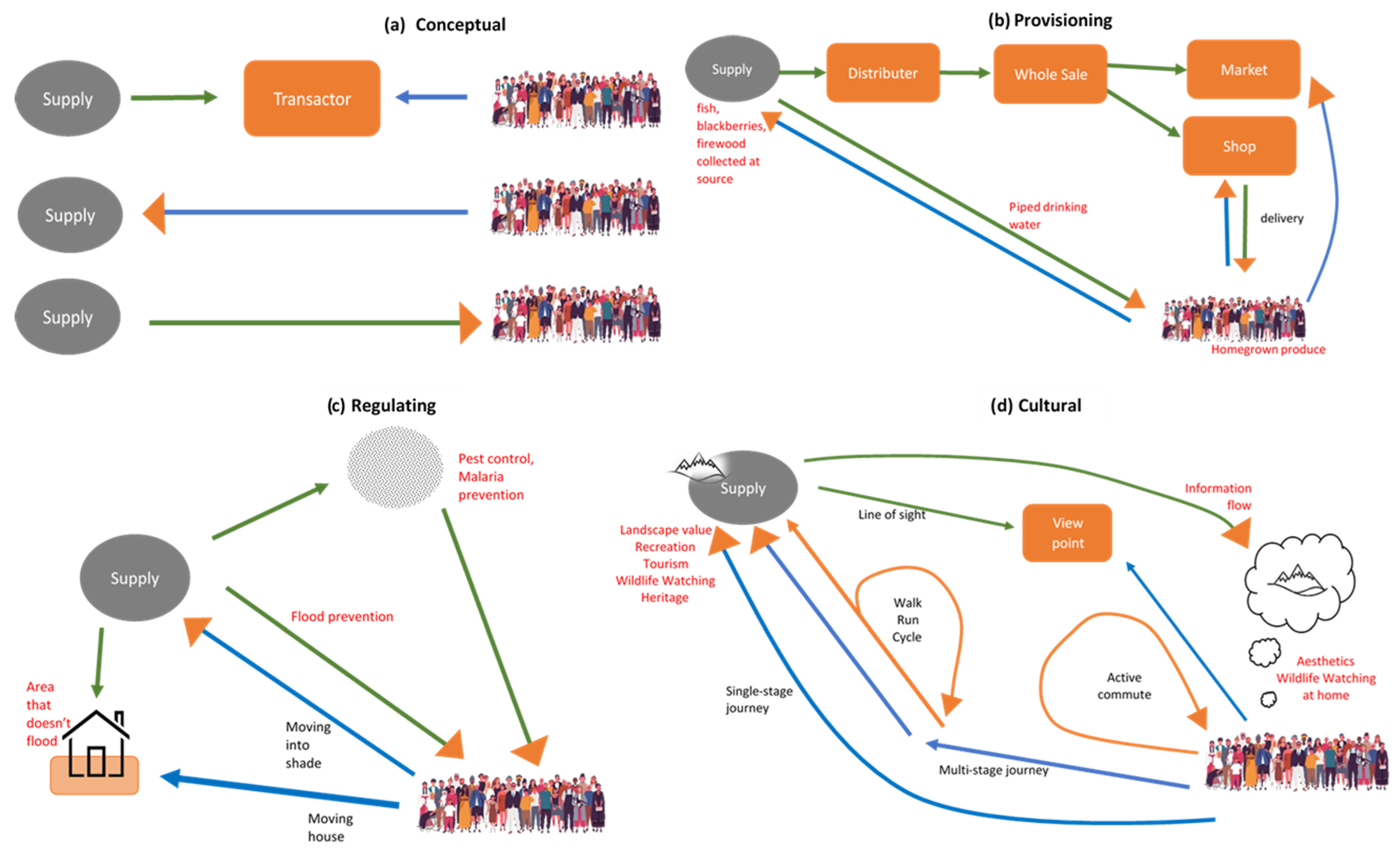
Figure 1. The flow of ecosystem services (ESs), conceptualised as two processes (a): nature to people (N2P; the movement of a natural good towards beneficiaries, shown in green) and people to nature (P2N; the movement of beneficiaries to a transactor in search of an ecosystem service, blue). Transactors, the point where the ES becomes realised, are shown in orange. Transactors are sometimes spatially distinct from the ecosystem and beneficiary (orange rectangles), but at other times the ‘transaction’ occurs in-situ (either at the ecosystem or beneficiary; orange arrowheads). Demand is shown via the group of people, with specific ES examples given in red. These processes occur across all ES categories: provisioning (b), regulating (c), and cultural (d). For example, drinking water flows down a mountain (N2P) and people go to the river to collect it (P2N). Sometimes P2N involves travelling all the way to the supply source, e.g., going to a forest to collect firewood, and sometimes N2P comes all the way to the demand, e.g., regulating services like pest control.
Land 10 00576 g001
Table 1. Mechanisms to describe ES flow, broken down into ‘nature to people’ (the movement of a natural good to a transactor, where it is used by beneficiaries) and ‘people to nature’ (the movement of beneficiaries to a transactor in search of an ecosystem service). Mechanisms are based on the work of Fisher, Turner and Morling [44], with more recent ES examples.
FlowMechanismExample of Ecosystem ServiceReference
Nature to people (N2P)In situ
Services are provided and accessed in the same area
Aesthetics—beautiful surroundings, with light flowing via the line of sight (cultural)
Existence value, accessed through media (cultural)
[25]
[45]
Gravitational
From uplands to lowlands
Flood regulation provided by forested slopes (regulating)[46]
Directional
Benefits flow in one direction
Pollination—from habitat to crops (regulating)[47]
Omni-directional
Benefits flow in all directions
Carbon storage—global benefit (regulating)[24]
People to nature
(P2N)
In Situ
Services accessed from base, no movement
needed
Gardens providing aesthetics, wildlife, sense of place (cultural)[48]
Single-stage journeyTo go to a park for recreation (cultural)
Journey itself may be the service—recreation (cultural)
[49]
Multi-stage journeyTo go to a National Park for recreation, wildlife watching. Journey may be by train, bus or taxi, then hiking (cultural)
Journey itself or one stage may be the service—recreation (cultural)
[37]
Active CommuteConnection with nature is not the primary aim of the journey[50]
Table 2. Summary of migration theories and potential applications to ‘people to nature’ (the movement of beneficiaries to a transactor in search of an ecosystem service).
TheoryDescriptionApplication to ‘People to Nature’
Push-pull-mooring (PPM) [55]
  • Push—negative factors that push an individual towards leaving an area
  • Pull—positive factors that attract people to somewhere new
  • Mooring—factors that may hinder or facilitate the move
  • Push factors—the local area is urban (too grey and manmade)
  • Pull factors—fresh air, nature, birdsong
  • Mooring factors—too far away, too expensive, family considerations
Inverse distance law [36]
  • Most migration is over short distances
  • Increased distance represents greater cost.
  • Cost may be linear or it may be proportional and involve ‘step-ups’ in cost.
  • People will access services close to where they live if available.
  • A linear increase in friction of distance would mean accessing a service further away.
  • Proportional jumps might include having to stay overnight to access an area.
Gravity model [36]
  • There is greater movement between areas of greater ‘mass’ i.e., attractiveness.
  • Distance decay means that for two sites of the same mass, there will be less movement to the further one.
  • ‘Mass’ here corresponds to greater ES potential, attractiveness and significance.
  • Significance can be increased, perpetuated by social media.
Law of intervening opportunities [67]
  • People will migrate to where opportunities are greatest.
  • The amount of migration is proportional to the opportunities at the destination and inversely proportional to opportunities between the starting point and the end destination.
  • An area that offers lots of opportunities to access ES would be the most desirable.
  • If there are areas closer that provide some of these opportunities, people may choose to go there as the cost is lower.
Radiation Model [68]
  • To decide where to migrate to, people score all possible opportunities based on how closely they match their desired experience
  • Then, they rank them based on how far they are, and the cost to access them.
  • People score all accessible locations based on how closely they provide the ES they want to access e.g., a walk in nature
  • Then, they rank them based on how far they are, and the cost to access them.
Table 3. Summary of foraging theories and potential applications to ‘people to nature’ (the movement of beneficiaries to a transactor in search of an ecosystem service).
TheoryDetailsApplication to ‘People to Nature’
Marginal Value Theorem
[80]
  • Individuals use the most energy-efficient method to move around their environment
  • Assumes resources are patchy
  • Assumes perfect knowledge
  • People have to access ESs, but will not necessarily use the most efficient route, especially if they do not know the area
  • ES provision is patchy within the landscape
Ideal Free Distribution
[86]
  • Individuals will distribute themselves proportionately based on the resources available.
  • Assumes perfect knowledge of patch quality
  • IFD might allow people to have the optimal experience
  • Realistically, distribution will likely be clumped around areas of easy access and high significance, especially if people are unfamiliar with the area.
Central Place Foraging
[81]
  • Individuals forage and then return to a central place
  • People accessing ESs from home and then returning home
  • Return journey has to be factored in
Movement Ecology Paradigm
[91]
  • Considers the internal state of the individual (why they move), how they move, their ability to navigate and external factors that might affect them.
  • Internal state: why do they want to seek a particular ES?
  • How: walk, cycle, drive? Multi-stage or one-stage journey? Is anything limiting movement?
  • Ability: Knowledge of the area, confidence
  • External factors: external pressures, other individuals, surroundings
Publisher’s Note: MDPI stays neutral with regard to jurisdictional claims in published maps and institutional affiliations.

