Numerical Analysis of an Osseointegration Model

Abstract

In this work, we study a bone remodeling model used to reproduce the phenomenon of osseointegration around endosseous implants. The biological problem is written in terms of the densities of platelets, osteogenic cells, and osteoblasts and the concentrations of two growth factors. Its variational formulation leads to a strongly coupled nonlinear system of parabolic variational equations. An existence and uniqueness result of this variational form is stated. Then, a fully discrete approximation of the problem is introduced by using the finite element method and a semi-implicit Euler scheme. A priori error estimates are obtained, and the linear convergence of the algorithm is derived under some suitable regularity conditions and tested with a numerical example. Finally, one- and two-dimensional numerical results are presented to demonstrate the accuracy of the algorithm and the behavior of the solution.

1. Introduction

The study of the phenomenon of osseointegration in endosseous implants is a very interesting issue because of the increasing use of many types of implants in clinical practice. Dental implantation stands out as the area that has benefited the most from the innovation and continuous development of bone implants in the last few years. This is probably due to the outstanding clinical results (see, e.g., [1]). These dental implants are artificial systems that consist of an endosteal component, which is completely inside the mandible, and an abutment that connects the endosseous component with the oral cavity, in order to replace a missing tooth [2].

The behavior of bone tissue depends on the chemical properties of the materials used on the implant and on the ability of the implant to introduce a mechanical state of stress, which induces the osteogenesis processes. Therefore, there are two possible ways to study this process. The first one involves clinical trials, where known failure mechanisms of implants are evaluated and their incidence assessed. The second one consists of preclinical studies, which allow performing a preliminary analysis of the system using computer tools.

Currently, the number of papers dealing with the numerical simulation of the behavior and stability of dental implants is huge (see, for instance, [3,4,5,6,7,8,9,10,11,12,13,14,15,16,17,18,19,20,21,22,23,24,25,26]). This work also follows the aforementioned research line about preclinical studies, continuing the studies already published in [27,28]. There, the authors presented a new biological model to predict the osseointegration of the implant in the bone. In the first part [27], they considered the full model, performing two-dimensional numerical simulations (implemented in ABAQUS) of the bone ingrowth process around the dental implant, assuming two different surface properties. Then, in the second part [28], two simplified versions of this problem were considered, providing a stability analysis and showing the existence of traveling wave-type solutions. In this work, we also continue the research started in [29,30] (where both simplified models were numerically analyzed) considering the full osseointegration model.

The paper is structured in the following way. The biological problem and its variational formulation are presented in Section 2. Then, fully discrete approximations are introduced in Section 3. We use the finite element method to approximate the spatial variable and an Euler scheme to discretize the time derivatives. A priori error estimates are then proven, from which the linear convergence is derived. Finally, one- and two-dimensional numerical simulations are presented in Section 4, where we show the accuracy of the numerical resolution and the behavior of the solution.

2. Biological Problem and Its Variational Formulation

In this section, a brief description of the model is presented. To obtain further details, we refer to the paper where the model was presented [27]. Denote by “·” and $\parallel ·\parallel$ the inner product and the Euclidean norm on ${\mathbb{R}}^d$. Let $\Omega \subset {\mathbb{R}}^d$, $d=1,2,3$, be a domain with a Lipschitz boundary $\Gamma =\partial \Omega$, which can be decomposed into two disjoint parts ${\Gamma }_1$ and ${\Gamma }_2$ such that $\mathrm{measure}\left({\Gamma }_1\right),\mathrm{measure}\left({\Gamma }_2\right)>0$. Let $[0,T]$, $T>0$, and $\mathit{\nu }={\left({\nu }_i\right)}_{i=1}^d$ represent the time interval of interest and the outward unit normal vector to $\Gamma$, respectively. Finally, let $\mathit{x}\in \Omega$ be the spatial variable and $t\in [0,T]$ the time variable. We do not indicate the dependence of the functions on them in order to simplify the writing.

According to [27], we describe the biological model in what follows. Once the surgical procedure is finished and the implant is placed, blood fills the cavity, and proteins and tissue fluids are absorbed into the implant surface. Then, platelets are activated due to the contact with the surface, and they release a number of growth factors. These growth factors stimulate the migration and proliferation of osteoblasts. Once these processes begin, the osteogenic cells coming from the old bone migrate to the surface of the implant, and they differentiate into osteoblasts, which later synthesize bone matrix.

Here, following [27], we assume that there are two generic growth factors. The first factor corresponds to the release of activated platelets (PGDF, TGF-$\beta$), and the second one accounts for the molecules secreted by osteoblasts and osteogenic cells (BMPs, TGF-$\beta$ superfamily).

First, let us denote by $c\in \mathbb{R}$ the density of platelets, whose evolution is determined as follows,

$$\frac{\partial c}{\partial t}-D_c\Delta c+A_{c}c=-\nabla ·H_{c}c\nabla p.$$

The evolution of c was modeled as a linear diffusion (multiplied by $D_c$), the cell adhesion to the implant surface, and a kinetic term. Cell adhesion was modeled with a linear “taxis” term depending on the gradient of adsorbed proteins $\nabla p$, with a coefficient $H_c$. We note that the value of p is assumed to be known, and it depends on the microtopography of the implant surface. Its maximum value appears at the surface of the implant and then decreases as we move away from this surface, reaching soon a value of zero that is maintained in the remaining domain [27]. We assume a high platelet concentration at the beginning, so the only kinetic term appears from cell removal due to inflammation, with a linear rate $A_c$.

Secondly, the density of the osteogenic cells, m, is modeled by the equation:

$$\begin{array}{c}{\displaystyle \frac{\partial m}{\partial t}-D_m\Delta m+A_{m}m=-\nabla ·m(B_{m1}\nabla s_1+B_{m2}\nabla s_2)-\frac{{\alpha }_{mb}{s}_1}{{\beta }_{mb}+s_1}m}\hfill \\ {\displaystyle +\left({\alpha }_{m0}+\frac{{\alpha }_m{s}_1}{{\beta }_m+s_1}+\frac{{\alpha }_m{s}_2}{{\beta }_m+s_2}\right)m\left(1-\frac{m}{N}\right).}\hfill \end{array}$$

Here, besides the linear diffusion and kinetics, there is a chemotaxis term along the gradients of the growth factors $s_1$ and $s_2$ and logistic growths with these factors. These growths are bounded by a limiting cell density N. Further explanations on the modeling can be found in the original reference.

Next, the density of osteoblasts b is modeled by the following equation:

$$\frac{\partial b}{\partial t}=\frac{{\alpha }_{mb}{s}_1}{{\beta }_{mb}+s_1}m-A_{b}b.$$

In this case, we obtain an ordinary differential equation instead of a partial differential one because osteoblasts remain on the surface of the bone matrix, so there is no flux of these cells. The source term comes from the differentiation from the osteogenic phenotype, and the decay accounts for differentiation into osteocytes $A_b$.

Finally, following [27], we describe the evolution of both generic growth factors $s_1$ and $s_2$. The first generic factor $s_1$ is assumed to satisfy the following constitutive partial differential equation:

$${\displaystyle \frac{\partial s_1}{\partial t}-D_{s1}\Delta s_1=\left(\frac{{\alpha }_{c1}p}{{\beta }_{c1}+p}+\frac{{\alpha }_{c2}{s}_1}{{\beta }_{c2}+s_1}\right)c-A_{s1}{s}_1.}$$

Again, random dispersion of this factor is modeled with a diffusive term with a linear coefficient $D_{s1}$. The kinetic term accounts for the secretion of $s_1$ by platelets (c) together with the concentration of the absorbed proteins p and the growth factor $s_1$ itself, both as logistic terms. As in the previous equations, a natural decay of the factor with linear rate $A_{s1}$ appears.

The second generic factor is assumed to satisfy a similar equation:

$${\displaystyle \frac{\partial s_2}{\partial t}-D_{s2}\Delta s_2=\frac{{\alpha }_{m2}{s}_2}{{\beta }_{m2}+s_2}m+\frac{{\alpha }_{b2}{s}_2}{{\beta }_{b2}+s_2}b-A_{s2}{s}_2.}$$

Now, there are two source terms depending on logistic functions of $s_2$ and concentrations of m and b. The natural decay is multiplied by the factor $A_{s2}$.

We note that these constitutive equations are nonlinear, and so, for mathematical reasons, some of the terms must be truncated. In order to do that, for some constants $M_1>0$ and $M_2>0$, we introduce the truncation operators $R_1:\mathbb{R}\to [0,M_1]$ and $R_2:\mathbb{R}\to [0,M_2]$ given by:

$$R_1\left(z\right)=\left\{\begin{array}{c}z\mathrm{if}z\in [0,M_1],\hfill \\ 0\mathrm{if}z<0,\hfill \\ M_1\mathrm{if}z>M_1,\hfill \end{array}\right.R_2\left(z\right)=\left\{\begin{array}{c}z\mathrm{if}z\in [0,M_2],\hfill \\ 0\mathrm{if}z<0,\hfill \\ M_2\mathrm{if}z>M_2.\hfill \end{array}\right.$$

Remark 1.

We point out that these truncation operators are introduced to assure some mathematical properties. Anyway, we note that, although we have not been able to prove these boundedness properties theoretically, in the bone remodeling processes, as well as in the performed numerical simulations, they were observed.

In order to simplify the writing, we define the following functions $f:{\mathbb{R}}^3\to \mathbb{R}$, $g:{\mathbb{R}}^2\to \mathbb{R}$, and $h:{\mathbb{R}}^3\to \mathbb{R}$:

$$\begin{array}{c}{\displaystyle f(m,s_1,s_2)=-\frac{{\alpha }_{mb}{s}_1}{{\beta }_{mb}+s_1}m+\left({\alpha }_{m0}+\frac{{\alpha }_m{s}_1}{{\beta }_m+s_1}+\frac{{\alpha }_m{s}_2}{{\beta }_m+s_2}\right)m\left(1-\frac{m}{N}\right),}\hfill \\ {\displaystyle g(s_1,c)=\left(\frac{{\alpha }_{c1}p}{{\beta }_{c1}+p}+\frac{{\alpha }_{c2}{s}_1}{{\beta }_{c2}+s_1}\right)c,}\hfill \\ {\displaystyle h(s_2,m,b)=\frac{{\alpha }_{m2}{s}_2}{{\beta }_{m2}+s_2}m+\frac{{\alpha }_{b2}{s}_2}{{\beta }_{b2}+s_2}b.}\hfill \end{array}$$

Concerning the boundary conditions for the density of the osteogenic cells m, we assume a known value on ${\Gamma }_1$ since there is a contribution from the bone. There is no flux through ${\Gamma }_2$. Moreover, we assume that there is no flux through the whole boundary $\Gamma$ for the remaining variables (density of platelets and generic growth factors).

Finally, we denote by $c_0$, $m_0$, $s_{10}$, $s_{20}$, and $b_0$ the initial conditions for $c,m,s_1,s_2$, and b, respectively. Collecting all these equations, the full bone integration problem is then written as follows.

Problem P.Find the density of platelets $c:\overline{\Omega }\times [0,T]\to \mathbb{R}$, the density of osteogenic cells $m:\overline{\Omega }\times [0,T]\to \mathbb{R}$, the concentration of the first growth factor $s_1:\overline{\Omega }\times [0,T]\to \mathbb{R}$, the concentration of the second growth factor $s_2:\overline{\Omega }\times [0,T]\to \mathbb{R}$, and the density of osteoblasts $b:\overline{\Omega }\times [0,T]\to \mathbb{R}$ such that,

$$\begin{array}{c}{\displaystyle \frac{\partial c}{\partial t}-D_c\Delta c+A_{c}c=-\nabla ·H_{c}c\nabla pin\Omega \times (0,T),}\hfill \end{array}$$

(1)

$$\begin{array}{c}\frac{\partial m}{\partial t}-D_m\Delta m+A_{m}m=-\nabla ·(B_{m_1}{R}_2\left(m\right)\nabla s_1+B_{m_2}{R}_2\left(m\right)\nabla s_2)\hfill \\ +f(R_2\left(m\right),R_1\left(s_1\right),R_1\left(s_2\right))in\Omega \times (0,T),\hfill \end{array}$$

(2)

$$\begin{array}{c}\frac{\partial s_1}{\partial t}-D_{s_1}\Delta s_1+A_{s_1}{s}_1=g(R_1\left(s_1\right),c)in\Omega \times (0,T),\hfill \end{array}$$

(3)

$$\begin{array}{c}\frac{\partial s_2}{\partial t}-D_{s_2}\Delta s_2+A_{s_2}{s}_2=h(m,R_1\left(s_2\right),b)in\Omega \times (0,T),\hfill \end{array}$$

(4)

$$\begin{array}{c}\frac{\partial b}{\partial t}+A_{b}b=\frac{{\alpha }_{mb}{R}_1\left(s_1\right)}{{\beta }_{mb}+R_1\left(s_1\right)}min\Omega \times (0,T),\hfill \end{array}$$

(5)

$$\begin{array}{c}m=m_{bone}on{\Gamma }_1\times (0,T),\hfill \end{array}$$

(6)

$$\begin{array}{c}\frac{\partial s_1}{\partial \mathit{\nu }}=\frac{\partial s_2}{\partial \mathit{\nu }}=\frac{\partial c}{\partial \mathit{\nu }}=0on{\Gamma }_1\times (0,T),\hfill \end{array}$$

(7)

$$\begin{array}{c}\frac{\partial m}{\partial \mathit{\nu }}=\frac{\partial s_1}{\partial \mathit{\nu }}=\frac{\partial s_2}{\partial \mathit{\nu }}=\frac{\partial c}{\partial \mathit{\nu }}=0on{\Gamma }_2\times (0,T),\hfill \end{array}$$

(8)

$$\begin{array}{c}c\left(0\right)=c_0,m\left(0\right)=m_0,s_1\left(0\right)=s_{1_0},s_2\left(0\right)=s_{2_0},b\left(0\right)=b_{0}in\Omega .\hfill \end{array}$$

(9)

Remark 2.

We note that in [27], the authors also derived the equations for the volume fractions of the fibrin network, the woven bone, and the lamellar bone, but they were obtained from the above densities and growth factors. Therefore, in this work, we did not consider them. However, it could be interesting to analyze the evolution of the mass density [31,32,33].

To obtain the variational formulation of Problem P, let $Y=L^2(\Omega )$, $H={\left[L^2(\Omega )\right]}^d$ and $E=H^1(\Omega )$, and denote by ${(·,·)}_Y$, ${(·,·)}_H$, and ${(·,·)}_E$ their respective scalar products, with corresponding norms ${\parallel ·\parallel }_Y$, ${\parallel ·\parallel }_H$, and ${\parallel ·\parallel }_E$.

Moreover, let us define the variational space V as follows,

$$V=\{v\in H^1(\Omega );v=0\mathrm{on}{\Gamma }_1\},$$

with scalar product ${(·,·)}_V$ and norm ${\parallel ·\parallel }_V$.

Integrating in time Equation (5) and using the initial condition (9), we obtain:

$$b(\mathit{x},t)=e^{-A_{b}t}\left[{\int }_0^t\frac{{\alpha }_{mb}{R}_1\left(s_1(\mathit{x},s)\right)}{{\beta }_{mb}+R_1\left(s_1(\mathit{x},s)\right)}m(\mathit{x},s)e^{A_{b}s}ds+b_0\left(\mathit{x}\right)\right].$$

(10)

Plugging Equation (10) into Equation (4), applying Green’s formula, and then using the boundary conditions (6)–(8), we derive the following variational formulation of Problem P, written in terms of densities c and m and concentrations $s_1$ and $s_2$.

Problem VP.Find the density of platelets $c:[0,T]\to E$, the density of osteoblasts $m:[0,T]\to V$, the concentration of the first growth factor $s_1:[0,T]\to E$, and the concentration of the second growth factor $s_2:[0,T]\to E$ such that $c\left(0\right)=c_0$, $m\left(0\right)=m_0$, $s_1\left(0\right)=s_{1_0}$, and $s_2\left(0\right)=s_{2_0}$, and, for a.e. $t\in (0,T)$ and for all $u\in V$, $v,w,z\in E$,

$$\begin{array}{c}{\left(\frac{\partial c}{\partial t}\left(t\right),v\right)}_Y+D_c{(\nabla c\left(t\right),\nabla v)}_H+A_c{(c\left(t\right),v)}_Y=H_c{(c\left(t\right)\nabla p\left(t\right),\nabla v)}_H,\hfill \end{array}$$

(11)

$$\begin{array}{c}{\left(\frac{\partial m}{\partial t}\left(t\right),u\right)}_Y+D_m{(\nabla m\left(t\right),\nabla u)}_H+A_m{(m\left(t\right),u)}_Y={(R_2\left(m\left(t\right)\right)[B_{m_1}\nabla s_1\left(t\right)+B_{m_2}\nabla s_2\left(t\right)],\nabla u)}_H\hfill \\ +(f(R_2\left(m\left(t\right)\right),R_1\left(s_1\left(t\right)\right)),R_1\left(s_2\left(t\right)\right)){,u)}_Y,\hfill \end{array}$$

(12)

$$\begin{array}{c}{\left(\frac{\partial s_1}{\partial t}\left(t\right),w\right)}_Y+D_{s_1}{(\nabla s_1\left(t\right),\nabla w)}_H+A_{s_1}{(s_1\left(t\right),w)}_Y={(g(R_1\left(s_1\left(t\right)\right),c\left(t\right)),w)}_Y,\hfill \end{array}$$

(13)

$$\begin{array}{c}{\left(\frac{\partial s_2}{\partial t}\left(t\right),z\right)}_Y+D_{s_2}{(\nabla s_2\left(t\right),\nabla z)}_H+A_{s_2}{(s_2\left(t\right),z)}_Y={(h(m\left(t\right),R_1\left(s_2\left(t\right)\right),b\left(t\right)),z)}_Y.\hfill \end{array}$$

(14)

In this variational problem, the density of osteoblasts b is obtained from (10).

In the following result, we state that the above problem has a unique weak solution.

Theorem 1.

If we assume that the constitutive coefficients $D_c$, $A_c$, $D_m$, $A_m$, $D_{s1}$, $A_{s1}$, $D_{s2}$, and $A_{s2}$ are strictly positive, then Problem VP admits a unique solution with the regularity:

$$c,m,s_1,s_2\in C^1([0,T];Y)\cap C([0,T];E).$$

The proof of the above theorem is rather technical, and it is based on well known results on evolution equations with monotone operators (see, for instance, [34,35,36]) and an application of the fixed-point theorem. We omit the details for the sake of reading.

3. Fully Discrete Approximations and an a Priori Error Analysis

In this section, we introduce a finite element algorithm to approximate solutions to Problem VP. Then, we also provide an a priori error analysis.

The discretization of Problem VP is performed as follows. First, we assume $\overline{\Omega }$ to be a polyhedral domain, and we consider two finite dimensional spaces $E^h\subset E$ and $V^h\subset V$, which approximate the variational spaces E and V, given by:

$$\begin{array}{c}{E}^h=\{u^h\in C\left(\overline{\Omega }\right);u_{{|}_K}^h\in P_1\left(K\right)K\in {\mathcal{T}}^h\},\hfill \end{array}$$

(15)

$$\begin{array}{c}{V}^h=\{v^h\in C\left(\overline{\Omega }\right);v_{{|}_K}^h\in P_1\left(K\right)K\in {\mathcal{T}}^h,v^h=0\mathrm{on}{\Gamma }_1\},\hfill \end{array}$$

(16)

where $P_1\left(K\right)$ represents the space of polynomials with a global degree less than or equal to one in K. Following [37], we denote by ${\left({\mathcal{T}}^h\right)}_{h>0}$ a regular family of triangulations of $\overline{\Omega }$, which is compatible with the partition of the boundary $\Gamma =\partial \Omega$ into ${\Gamma }_1$ and ${\Gamma }_2$. Therefore, the finite element spaces $E^h$ and $V^h$ are composed of functions that are continuous and piecewise affine. Let $h_K$ be the diameter of an element $K\in {\mathcal{T}}^h$ so ${\displaystyle h=\underset{K\in {\mathcal{T}}^h}{max}{h}_K}$ denotes the spatial discretization parameter. Moreover, we assume that the discrete initial conditions, denoted by $c_0^h$, $m_0^h$, $s_{1_0}^h$, and $s_{2_0}^h$, are given by:

$$c_0^h={\mathcal{P}}^h{c}_0,m_0^h={\mathcal{P}}^h{m}_0,s_{1_0}^h={\mathcal{P}}^h{s}_{1_0},s_{2_0}^h={\mathcal{P}}^h{s}_{2_0},$$

(17)

where ${\mathcal{P}}^h$ is the $L^2(\Omega )$-projection operator over $E^h$.

To obtain a discretization of the time derivatives, let $0=t_0<t_1<\dots <t_N=T$ be a uniform partition of the time interval $[0,T]$, and we define k as the time step size given by $k=T/N$. If $r\left(t\right)$ is a continuous function, then we define $r_n=r\left(t_n\right)$, and for a sequence ${\left\{w_n\right\}}_{n=0}^N$, we let $\delta w_n=(w_n-w_{n-1})/k$ be its usual divided differences.

Therefore, using a Euler scheme, we obtain the following fully discrete approximation of Problem VP.

Problem${\mathbf{VP}}^{\mathit{h}\mathit{k}}$.Find the discrete density of platelets $c^{hk}={\left\{c_n^{hk}\right\}}_{n=0}^N\subset E^h$, the discrete density of osteoblasts $m^{hk}={\left\{m_n^{hk}\right\}}_{n=0}^N\subset V^h$, the discrete concentration of the first growth factor $s_1^{hk}={\left\{s_{1_n}^{hk}\right\}}_{n=0}^N\subset E^h$, and the discrete concentration of the second growth factor $s_2^{hk}={\left\{s_{2_n}^{hk}\right\}}_{n=0}^N\subset E^h$ such that $c_0^{hk}=c_0^h$, $m_0^{hk}=m_0^h$, $s_{1_0}^{hk}=s_{1_0}^h$, and $s_{2_0}^{hk}=s_{2_0}^h$, and, for $n=1,\dots ,N$ and for all $u^h\in V^h$ and $v^h,w^h,z^h\in E^h$,

$$\begin{array}{c}{\left(\delta c_n^{hk},v^h\right)}_Y+D_c{(\nabla c_n^{hk},\nabla v^h)}_H+A_c{(c_n^{hk},v^h)}_Y=H_c{(c_{n-1}^{hk}\nabla p_n,\nabla v^h)}_H,\hfill \end{array}$$

(18)

$$\begin{array}{c}{\left(\delta m_n^{hk},u^h\right)}_Y+D_m{(\nabla m_n^{hk},\nabla u^h)}_H+A_m{(m_n^{hk},u^h)}_Y={(R_2\left(m_{n-1}^{hk}\right)[B_{m_1}\nabla s_{1_{n-1}}^{hk}+B_{m_2}\nabla s_{2_{n-1}}^{hk}],\nabla u^h)}_H\hfill \\ +{(f(R_2\left(m_{n-1}^{hk}\right),R_1\left(s_{1_{n-1}}^{hk}\right),R_1\left(s_{2_{n-1}}^{hk}\right)),u^h)}_Y,\hfill \end{array}$$

(19)

$$\begin{array}{c}{\left(\delta s_{1_n}^{hk},w^h\right)}_Y+D_{s_1}{(\nabla s_{1_n}^{hk},\nabla w^h)}_H+A_{s_1}{(s_{1_n}^{hk},w^h)}_Y={(g(R_1\left(s_{1_{n-1}}^{hk}\right),c_{n-1}^{hk}),w^h)}_Y,\hfill \end{array}$$

(20)

$$\begin{array}{c}{\left(\delta s_{2_n}^{hk},z^h\right)}_Y+D_{s_2}{(\nabla s_{2_n}^{hk},\nabla z^h)}_H+A_{s_2}{(s_{2_n}^{hk},z^h)}_Y={(h(m_{n-1}^{hk},R_1\left(s_{2_{n-1}}^{hk}\right),b_{n-1}^{hk}),z^h)}_Y,\hfill \end{array}$$

(21)

where the discrete density of osteoblasts $b^{hk}={\left\{b_n^{hk}\right\}}_{n=0}^N$ is given by:

$$b_n^{hk}=e^{-A_b{t}_n}\left[b_0^h+k\sum _{j=1}^n\frac{{\alpha }_{mb}{R}_1\left(s_{1_j}^{hk}\right)}{{\beta }_{mb}+R_1\left(s_{1_j}^{hk}\right)}{m}_j^{hk}{e}^{A_b{t}_j}\right],$$

(22)

and$b_0^h={\mathcal{P}}^h{b}_0$.

We note that we have used the explicit expression in the nonlinear terms in order to simplify the numerical resolution of this discrete problem.

Since the resulting equations of Problem ${\mathrm{VP}}^{hk}$ are now uncoupled because they can be solved separately, using Lax–Milgram lemma, it is easy to obtain the existence of a unique discrete solution $c^{hk}\subset E^h$, $m^{hk}\subset V^h$, $s_1^{hk}\subset E^h$, and $s_2^{hk}\subset E^h$ to Problem ${\mathrm{VP}}^{hk}$.

Now, we derive some a priori estimates for the numerical errors $c_n-c_n^{hk}$, $m_n-m_n^{hk}$, $s_{1_n}-s_{1_n}^{hk}$ $s_{2_n}-s_{2_n}^{hk}$, and $b_n-b_n^{hk}$. Thus, we assume that Problem VP has a unique solution with the following regularity:

$$\begin{array}{c}m\in C^1([0,T];Y)\cap C([0,T];V\cap L^{\infty }\left(\overline{\Omega }\right)),b\in C^1([0,T];Y),\hfill \\ c,s_1,s_2\in C^1([0,T];Y)\cap C([0,T];E\cap W^{1,\infty }\left(\overline{\Omega }\right)).\hfill \end{array}$$

(23)

For the sake of simplicity, we assume that all the constants involved in Problems VP and ${\mathrm{VP}}^{hk}$ are equal to one; i.e., $A_c=D_c=H_c=1$, $D_m=A_m=B_{m_1}=B_{m_2}={\alpha }_{mb}={\beta }_{mb}={\alpha }_{m0}={\beta }_m={\alpha }_m=1$, $D_{s_1}=A_{s_1}={\alpha }_{c1}={\alpha }_{c2}={\beta }_{c1}={\beta }_{c2}=1$, $D_{s_2}=A_{s_2}={\alpha }_{m2}={\alpha }_{b2}={\beta }_{m2}={\beta }_{b2}=1$, and $A_b=1$. We note that it is immediate to extend the results presented below to the general case.

First, we obtain some estimates on the density of osteoblasts. Then, we subtract Equation (10) at time $t=t_n$ and Equation (22) to obtain:

$$\parallel b_n-b_n^{hk}{\parallel }_Y\le C\left(\parallel b_0-b_0^h{\parallel }_Y+I_n+\sum _{j=1}^{n}k\left[\parallel m_j-m_j^{hk}{\parallel }_Y+{\parallel s_{1_j}-s_{1_j}^{hk}\parallel }_Y\right]\right),$$

(24)

where, here and in what follows, $C>0$ is a positive constant that depends on the data of the problem and the continuous solution; however, it is independent of the discretization parameters h and k, and $I_n$ is the integration error given by:

$$I_n={∥{\int }_0^{t_n}\frac{R_1\left(s_1\left(s\right)\right)}{R_1\left(s_1\left(s\right)\right)+1}m\left(s\right)e^{s-t_n}ds-k\sum _{j=1}^n\frac{R_1\left(s_{1_j}\right)}{R_1\left(s_{1_j}\right)+1}{m}_j{e}^{t_j-t_n}∥}_Y.$$

(25)

Then, we obtain some error estimates for the density of the platelets c. Finally, we subtract the variational Equation (11) at time $t=t_n$ and the discrete variational Equation (18) for a test function $v=v^h\in E^h$, obtaining:

$$\begin{array}{c}{\displaystyle {\left(\frac{\partial c}{\partial t}\left(t_n\right)-\delta c_n^{hk},v^h\right)}_Y+D_c{(\nabla (c_n-c_n^{hk}),\nabla v^h)}_H+A_c{(c_n-c_n^{hk},v^h)}_Y=H_c{((c_n-c_{n-1}^{hk})\nabla p_n,\nabla v^h)}_H.}\hfill \end{array}$$

Thus,

$$\begin{array}{c}{\displaystyle {\left(\frac{\partial c}{\partial t}\left(t_n\right)-\delta c_n^{hk},c_n-c_n^{hk}\right)}_Y+D_c{(\nabla (c_n-c_n^{hk}),\nabla (c_n-c_n^{hk}))}_H+A_c{(c_n-c_n^{hk},c_n-c_n^{hk})}_Y}\hfill \\ -H_c{((c_n-c_{n-1}^{hk})\nabla p_n,\nabla (c_n-c_n^{hk}))}_H\hfill \\ {\displaystyle ={\left(\frac{\partial c}{\partial t}\left(t_n\right)-\delta c_n^{hk},c_n-v^h\right)}_Y+D_c{(\nabla (c_n-c_n^{hk}),\nabla (c_n-v^h))}_H+A_c{(c_n-c_n^{hk},c_n-v^h)}_Y}\hfill \\ -H_c{((c_n-c_{n-1}^{hk})\nabla p_n,\nabla (c_n-v^h))}_H.\hfill \end{array}$$

Using the following property of the divided differences:

$$\begin{array}{c}{\left(\frac{\partial c}{\partial t}\left(t_n\right)-\delta c_n^{hk},c_n-c_n^{hk}\right)}_Y\hfill \\ {\displaystyle ={\left(\frac{\partial c}{\partial t}\left(t_n\right)-\delta c_n,c_n-c_n^{hk}\right)}_Y+{(\delta c_n-\delta c_n^{hk},c_n-c_n^{hk})}_Y}\hfill \\ {\displaystyle \ge {\left(\frac{\partial c}{\partial t}\left(t_n\right)-\delta c_n,c_n-c_n^{hk}\right)}_Y+\frac{1}{2k}\left(\parallel c_n-c_n^{hk}{\parallel }_Y^2-{\parallel c_{n-1}-c_{n-1}^{hk}\parallel }_Y^2\right),}\hfill \end{array}$$

where the notation $\delta c_n=(c_n-c_{n-1})/k$ represents the corresponding divided differences, and applying several times Young’s inequality:

$${\displaystyle ab\le ϵa^2+\frac{1}{4ϵ}{b}^2,a,b,ϵ\in \mathbb{R},ϵ>0,}$$

(26)

we have, for all $v^h\in E^h$,

$$\begin{array}{c}{\displaystyle \parallel c_n-c_n^{hk}{\parallel }_Y^2+Ck\parallel \nabla (c_n-c_n^{hk}){\parallel }_H^2+Ck{\parallel c_n-c_n^{hk}\parallel }_Y^2\le Ck({∥\frac{\partial c}{\partial t}\left(t_n\right)-\delta c_n∥}_Y^2+{(\delta c_n-\delta c_n^{hk},c_n-v^h)}_Y}\hfill \\ +\parallel c_n-v^h{\parallel }_E^2+\parallel c_n-c_n^{hk}{\parallel }_Y^2+\parallel c_n-c_{n-1}^{hk}{\parallel }_Y^2)+{\parallel c_{n-1}-c_{n-1}^{hk}\parallel }_Y^2.\hfill \end{array}$$

Thus, by induction, it follows that, for all $v^h={\left\{v_j^h\right\}}_{j=0}^n\subset E^h$,

$$\begin{array}{c}{\displaystyle \parallel c_n-c_n^{hk}{\parallel }_Y^2+Ck\sum _{j=1}^n\left[\parallel \nabla (c_j-c_j^{hk}){\parallel }_H^2+{\parallel c_j-c_j^{hk}\parallel }_Y^2\right]\le Ck\sum _{j=1}^n({∥\frac{\partial c}{\partial t}\left(t_j\right)-\delta c_j∥}_Y^2+{\parallel c_j-v_j^h\parallel }_E^2}\hfill \\ +{(\delta c_j-\delta c_j^{hk},c_j-v_j^h)}_Y+k^2+\parallel c_j-c_j^{hk}{\parallel }_Y^2)+{\parallel c_0-c_0^h\parallel }_Y^2,\hfill \end{array}$$

(27)

where we used the regularity $c\in C^1([0,T];Y).$

Now, we obtain the estimates on the density of osteoblasts m. Therefore, subtracting the variational Equation (12) at time $t=t_n$ for a test function $v=v^h\in V^h\subset V$ and the discrete variational Equation (19), we find that:

$$\begin{array}{c}{\displaystyle {\left(\frac{\partial m}{\partial t}\left(t_n\right)-\delta m_n^{hk},u^h\right)}_Y+D_m{(\nabla (m_n-m_n^{hk}),\nabla u^h)}_H+A_m{(m_n-m_n^{hk},u^h)}_Y}\hfill \\ ={(R_2\left(m_n\right)[B_{m_1}\nabla s_{1_n}+B_{m_2}\nabla s_{2_n}]-R_2\left(m_{n-1}^{hk}\right)[B_{m_1}\nabla s_{1_{n-1}}^{hk}+B_{m_2}\nabla s_{2_{n-1}}^{hk}],\nabla u^h)}_H\hfill \\ +{(f(R_2\left(m_n\right),R_1\left(s_{1_n}\right),R_1\left(s_{2_n}\right))-f(R_2\left(m_{n-1}^{hk}\right),R_1\left(s_{1_{n-1}}^{hk}\right),R_1\left(s_{2_{n-1}}^{hk}\right)),u^h)}_Y,\hfill \end{array}$$

and so,

$$\begin{array}{c}{\displaystyle {\left(\frac{\partial m}{\partial t}\left(t_n\right)-\delta m_n^{hk},m_n-m_n^{hk}\right)}_Y+D_m{(\nabla (m_n-m_n^{hk}),\nabla (m_n-m_n^{hk}))}_H+A_m{(m_n-m_n^{hk},m_n-m_n^{hk})}_Y}\hfill \\ -{(R_2\left(m_n\right)[B_{m_1}\nabla s_{1_n}+B_{m_2}\nabla s_{2_n}]-R_2\left(m_{n-1}^{hk}\right)[B_{m_1}\nabla s_{1_{n-1}}^{hk}+B_{m_2}\nabla s_{2_{n-1}}^{hk}],\nabla (m_n-m_n^{hk}))}_H\hfill \\ -{(f(R_2\left(m_n\right),R_1\left(s_{1_n}\right),R_1\left(s_{2_n}\right))-f(R_2\left(m_{n-1}^{hk}\right),R_1\left(s_{1_{n-1}}^{hk}\right),R_1\left(s_{2_{n-1}}^{hk}\right)),m_n-m_n^{hk})}_Y\hfill \\ {\displaystyle ={\left(\frac{\partial m}{\partial t}\left(t_n\right)-\delta m_n^{hk},m_n-u^h\right)}_Y+D_m{(\nabla (m_n-m_n^{hk}),\nabla (m_n-u^h))}_H+A_m{(m_n-m_n^{hk},m_n-u^h)}_Y}\hfill \\ -{(R_2\left(m_n\right)[B_{m_1}\nabla s_{1_n}+B_{m_2}\nabla s_{2_n}]-R_2\left(m_{n-1}^{hk}\right)[B_{m_1}\nabla s_{1_{n-1}}^{hk}+B_{m_2}\nabla s_{2_{n-1}}^{hk}],\nabla (m_n-u^h))}_H\hfill \\ -{(f(R_2\left(m_n\right),R_1\left(s_{1_n}\right),R_1\left(s_{2_n}\right))-f(R_2\left(m_{n-1}^{hk}\right),R_1\left(s_{1_{n-1}}^{hk}\right),R_1\left(s_{2_{n-1}}^{hk}\right)),m_n-u^h)}_Y.\hfill \end{array}$$

Taking into account that:

$$\begin{array}{c}{\left(\frac{\partial m}{\partial t}\left(t_n\right)-\delta m_n^{hk},m_n-m_n^{hk}\right)}_Y={\left(\frac{\partial m}{\partial t}\left(t_n\right)-\delta m_n,m_n-m_n^{hk}\right)}_Y+{(\delta m_n-\delta m_n^{hk},m_n-m_n^{hk})}_Y\hfill \\ {\displaystyle \ge {\left(\frac{\partial m}{\partial t}\left(t_n\right)-\delta m_n,m_n-m_n^{hk}\right)}_Y+\frac{1}{2k}\left(\parallel m_n-m_n^{hk}{\parallel }_Y^2-{\parallel m_{n-1}-m_{n-1}^{hk}\parallel }_Y^2\right),}\hfill \\ {(R_2\left(m_n\right)[B_{m_1}\nabla s_{1_n}+B_{m_2}\nabla s_{2_n}]-R_2\left(m_{n-1}^{hk}\right)[B_{m_1}\nabla s_{1_{n-1}}^{hk}+B_{m_2}\nabla s_{2_{n-1}}^{hk}],\nabla w)}_H\hfill \\ \le C\left(\parallel m_n-m_{n-1}^{hk}{\parallel }_Y^2+\parallel \nabla (s_{1_n}-s_{1_{n-1}}^{hk}){\parallel }_H^2+\parallel \nabla (s_{2_n}-s_{2_{n-1}}^{hk}){\parallel }_H^2\right),\hfill \\ \parallel f(R_2\left(m_n\right),R_1\left(s_{1_n}\right),R_1\left(s_{2_n}\right))-f(R_2\left(m_{n-1}^{hk}\right),R_1\left(s_{1_{n-1}}^{hk}\right),R_1\left(s_{2_{n-1}}^{hk}\right)){\parallel }_Y\hfill \\ \le C\left(\parallel m_n-m_{n-1}^{hk}{\parallel }_Y+\parallel s_{1_n}-s_{1_{n-1}}^{hk}{\parallel }_Y+{\parallel s_{2_n}-s_{2_{n-1}}^{hk}\parallel }_Y\right),\hfill \end{array}$$

where we have used the notation $\delta m_n=(m_n-m_{n-1})/k$, the properties of the truncation operators $R_1$ and $R_2$, and the expression of function f, and applying several times inequality (26), it follows that, for all $u^h\in V^h$,

$$\begin{array}{c}{\displaystyle \parallel m_n-m_n^{hk}{\parallel }_Y^2+Ck\parallel \nabla (m_n-m_n^{hk}){\parallel }_H^2+Ck\parallel m_n-m_n^{hk}{\parallel }_Y^2\le Ck({∥\frac{\partial m}{\partial t}\left(t_n\right)-\delta m_n∥}_Y^2+{\parallel m_n-u^h\parallel }_V^2}\hfill \\ +{(\delta m_n-\delta m_n^{hk},m_n-u^h)}_Y+\parallel m_n-m_{n-1}^{hk}{\parallel }_Y^2+\parallel \nabla (s_{1_n}-s_{1_{n-1}}^{hk}){\parallel }_H^2+\parallel \nabla (s_{2_n}-s_{2_{n-1}}^{hk}){\parallel }_H^2\hfill \\ +\parallel s_{1_n}-s_{1_{n-1}}^{hk}{\parallel }_Y^2+\parallel s_{2_n}-s_{2_{n-1}}^{hk}{\parallel }_Y^2)+{\parallel m_{n-1}-m_{n-1}^{hk}\parallel }_Y^2.\hfill \end{array}$$

Summing up to n, keeping in mind that $m\in C^1([0,T];Y)$, we find that, for all ${\left\{w_j^h\right\}}_{j=0}^n\subset V^h$,

$$\begin{array}{c}{\displaystyle \parallel m_n-m_n^{hk}{\parallel }_Y^2+Ck\sum _{j=1}^n\left[\parallel \nabla (m_j-m_j^{hk}){\parallel }_H^2+{\parallel m_j-m_j^{hk}\parallel }_Y^2\right]\le Ck\sum _{j=1}^n({∥\frac{\partial m}{\partial t}\left(t_j\right)-\delta m_j∥}_Y^2+{\parallel m_j-u_j^h\parallel }_V^2}\hfill \\ +{(\delta m_j-\delta m_j^{hk},m_j-u_j^h)}_Y+\parallel m_j-m_j^{hk}{\parallel }_Y^2+\parallel \nabla (s_{1_j}-s_{1_j}^{hk}){\parallel }_H^2+\parallel \nabla (s_{2_j}-s_{2_j}^{hk}){\parallel }_H^2\hfill \\ +k^2+\parallel s_{1_j}-s_{1_j}^{hk}{\parallel }_Y^2+{\parallel s_{2_j}-s_{2_j}^{hk}\parallel }_Y^2)+C\left(\parallel m_0-m_0^h{\parallel }_Y^2+\parallel s_{1_0}-s_{1_0}^h{\parallel }_E^2+{\parallel s_{2_0}-s_{2_0}^h\parallel }_E^2\right).\hfill \end{array}$$

(28)

Finally, we estimate the numerical errors on the concentration of the first and second growth factor, $s_1$ and $s_2$, respectively. Then, subtracting the variational Equation (13) at time $t=t_n$ for a test function $w=w^h\in E^h\subset E$ and the discrete variational Equation (20), we have, for all $w^h\in E^h$,

$$\begin{array}{c}{\displaystyle {\left(\frac{\partial s_1}{\partial t}\left(t_n\right)-\delta s_{1_n}^{hk},w^h\right)}_Y+D_{s_1}{(\nabla (s_{1_n}-s_{1_n}^{hk}),\nabla w^h)}_H+A_{s_1}{(s_{1_n}-s_{1_n}^{hk},w^h)}_Y}\hfill \\ ={(g(R_1\left(s_{1_n}\right),c_n)-g(R_1\left(s_{1_{n-1}}^{hk}\right),c_{n-1}^{hk}),w^h)}_Y.\hfill \end{array}$$

Therefore, we find that:

$$\begin{array}{c}{\displaystyle {\left(\frac{\partial s_1}{\partial t}\left(t_n\right)-\delta s_{1_n}^{hk},s_{1_n}-s_{1_n}^{hk}\right)}_Y+D_{s_1}{(\nabla (s_{1_n}-s_{1_n}^{hk}),\nabla (s_{1_n}-s_{1_n}^{hk}))}_H+A_{s_1}{(s_{1_n}-s_{1_n}^{hk},s_{1_n}-s_{1_n}^{hk})}_Y}\hfill \\ -{(g(R_1\left(s_{1_n}\right),c_n)-g(R_1\left(s_{1_{n-1}}^{hk}\right),c_{n-1}^{hk}),s_{1_n}-s_{1_n}^{hk})}_Y\hfill \\ {\displaystyle ={\left(\frac{\partial s_1}{\partial t}\left(t_n\right)-\delta s_{1_n}^{hk},s_{1_n}-w^h\right)}_Y+D_{s_1}{(\nabla (s_{1_n}-s_{1_n}^{hk}),\nabla (s_{1_n}-w^h))}_H+A_{s_1}{(s_{1_n}-s_{1_n}^{hk},s_{1_n}-w^h)}_Y}\hfill \\ -{(g(R_1\left(s_{1_n}\right),c_n)-g(R_1\left(s_{1_{n-1}}^{hk}\right),c_{n-1}^{hk}),s_{1_n}-w^h)}_Y.\hfill \end{array}$$

Taking into account that:

$$\begin{array}{c}{\left(\frac{\partial s_1}{\partial t}\left(t_n\right)-\delta s_{1_n}^{hk},s_{1_n}-s_{1_n}^{hk}\right)}_Y={\left(\frac{\partial s_1}{\partial t}\left(t_n\right)-\delta s_{1_n},s_{1_n}-s_{1_n}^{hk}\right)}_Y+{(\delta s_{1_n}-\delta s_{1_n}^{hk},s_{1_n}-s_{1_n}^{hk})}_Y\hfill \\ {\displaystyle \ge {\left(\frac{\partial s_1}{\partial t}\left(t_n\right)-\delta s_{1_n},s_{1_n}-s_{1_n}^{hk}\right)}_Y+\frac{1}{2k}\left(\parallel s_{1_n}-s_{1_n}^{hk}{\parallel }_Y^2-{\parallel s_{1_n-1}-s_{1_n-1}^{hk}\parallel }_Y^2\right),}\hfill \\ \parallel g(R_1\left(s_{1_n}\right),c_n)-g(R_1\left(s_{1_{n-1}}^{hk}\right),c_{n-1}^{hk}){\parallel }_Y\le C\left(\parallel s_{1_n}-s_{1_{n-1}}^{hk}{\parallel }_Y+{\parallel c_n-c_{n-1}^{hk}\parallel }_Y\right),\hfill \end{array}$$

where we have used the notation $\delta s_{1_n}=(s_{1_n}-s_{1_{n-1}})/k$, the properties of the truncation operator $R_1$, and the expression of function g, and applying several times inequality (26), it follows that, for all $w^h\in E^h$,

$$\begin{array}{c}{\displaystyle \parallel s_{1_n}-s_{1_n}^{hk}{\parallel }_Y^2+Ck\parallel \nabla (s_{1_n}-s_{1_n}^{hk}){\parallel }_H^2+Ck\parallel s_{1_n}-s_{1_n}^{hk}{\parallel }_Y^2\le Ck({∥\frac{\partial s_1}{\partial t}\left(t_n\right)-\delta s_{1_n}∥}_Y^2+{\parallel s_{1_n}-w^h\parallel }_E^2}\hfill \\ +{(\delta s_{1_n}-\delta s_{1_n}^{hk},s_{1_n}-w^h)}_Y+\parallel c_n-c_{n-1}^{hk}{\parallel }_Y^2)+{\parallel s_{1_{n-1}}-s_{1_{n-1}}^{hk}\parallel }_Y^2.\hfill \end{array}$$

Therefore, summing up to n, since $s_1\in C^1([0,T];Y)$ we have, for all ${\left\{w_j^h\right\}}_{j=0}^n\subset E^h$,

$$\begin{array}{c}{\displaystyle \parallel s_{1_n}-s_{1_n}^{hk}{\parallel }_Y^2+Ck\sum _{j=1}^n\left[\parallel \nabla (s_{1_j}-s_{1_j}^{hk}){\parallel }_H^2+{\parallel s_{1_j}-s_{1_j}^{hk}\parallel }_Y^2\right]\le Ck\sum _{j=1}^n({∥\frac{\partial s_1}{\partial t}\left(t_j\right)-\delta s_{1_j}∥}_Y^2+{\parallel s_{1_j}-w_j^h\parallel }_E^2}\hfill \\ +{(\delta s_{1_j}-\delta s_{1_j}^{hk},s_{1_j}-w_j^h)}_Y+\parallel c_j-c_j^{hk}{\parallel }_Y^2+k^2)+C\parallel s_{1_0}-s_{1_0}^h{\parallel }_Y^2+C{\parallel c_0-c_0^h\parallel }_Y^2.\hfill \end{array}$$

(29)

Proceeding in a similar way, we obtain the following estimates for concentration $s_2$, for all ${\left\{z_j^h\right\}}_{j=0}^n\subset E^h$,

$$\begin{array}{c}{\displaystyle \parallel s_{2_n}-s_{2_n}^{hk}{\parallel }_Y^2+Ck\sum _{j=1}^n\left[\parallel \nabla (s_{2_j}-s_{2_j}^{hk}){\parallel }_H^2+{\parallel s_{2_j}-s_{2_j}^{hk}\parallel }_Y^2\right]\le Ck\sum _{j=1}^n({∥\frac{\partial s_2}{\partial t}\left(t_j\right)-\delta s_{2_j}∥}_Y^2+{\parallel s_{2_j}-z_j^h\parallel }_E^2}\hfill \\ +{(\delta s_{2_j}-\delta s_{2_j}^{hk},s_{2_j}-z_j^h)}_Y+\parallel m_j-m_j^{hk}{\parallel }_Y^2+k^2+\parallel b_j-b_j^{hk}{\parallel }_Y^2)+C\parallel s_{2_0}-s_{2_0}^h{\parallel }_Y^2+C{\parallel m_0-m_0^h\parallel }_Y^2\hfill \\ +C\parallel b_0-b_0^h{\parallel }_Y^2.\hfill \end{array}$$

(30)

Combining now the estimates (24)–(30) and keeping in mind that (see [38]):

$$\begin{array}{c}{\displaystyle k\sum _{j=1}^n{(\delta c_j-\delta c_j^{hk},c_j-v_j^h)}_Y={(c_n-c_n^{hk},c_n-v_n^h)}_Y+{(c_0^h-c_0,c_1-v_1^h)}_Y}\hfill \\ {\displaystyle +\sum _{j=1}^{n-1}{(c_j-c_j^{hk},c_j-v_j^h-(c_{j+1}-v_{j+1}^h))}_Y,}\hfill \end{array}$$

$$\begin{array}{c}{\displaystyle k\sum _{j=1}^n{(\delta m_j-\delta m_j^{hk},m_j-u_j^h)}_Y={(m_n-m_n^{hk},m_n-u_n^h)}_Y+{(m_0^h-m_0,m_1-u_1^h)}_Y}\hfill \\ {\displaystyle +\sum _{j=1}^{n-1}{(m_j-m_j^{hk},m_j-u_j^h-(m_{j+1}-u_{j+1}^h))}_Y,}\hfill \\ {\displaystyle k\sum _{j=1}^n{(\delta s_{1_j}-\delta s_{1_j}^{hk},s_{1_j}-w_j^h)}_Y={(s_{1_n}-s_{1_n}^{hk},s_{1_n}-w_n^h)}_Y+{(s_{1_0}^h-s_{1_0},s_{1_1}-w_1^h)}_Y}\hfill \\ {\displaystyle +\sum _{j=1}^{n-1}{(s_{1_j}-s_{1_j}^{hk},s_{1_j}-w_j^h-(s_{1_{j+1}}-w_{j+1}^h))}_Y,}\hfill \\ {\displaystyle k\sum _{j=1}^n{(\delta s_{2_j}-\delta s_{2_j}^{hk},s_{2_j}-z_j^h)}_Y={(s_{2_n}-s_{2_n}^{hk},s_{2_n}-z_n^h)}_Y+{(s_{2_0}^h-s_{2_0},s_{2_1}-z_1^h)}_Y}\hfill \\ {\displaystyle +\sum _{j=1}^{n-1}{(s_{2_j}-s_{2_j}^{hk},s_{2_j}-z_j^h-(s_{2_{j+1}}-z_{j+1}^h))}_Y,}\hfill \end{array}$$

using the discrete version of Gronwall’s inequality (see [39]), we reach the following a priori error estimate result.

Theorem 2.

Let the assumptions of Theorem 1 hold. Assume that Problem $VP$ has the additional regularity (23), and let us denote by $(c,m,s_1,s_2,b)$ and $(c^{hk},m^{hk},s_1^{hk},s_2^{hk},b^{hk})$ the solutions to problems $VP$ and $V{P}^{hk}$, respectively. Therefore, we obtain that there exists a positive constant $C>0$, assumed to be independent of the discretization parameters h and k, but depending on the solution $(c,m,s_1,s_2,b)$ and the problem data, such that, for all ${\left\{u_n^h\right\}}_{n=0}^N\subset V^h$ and ${\left\{v_n^h\right\}}_{n=0}^N,{\left\{w_n^h\right\}}_{n=0}^N,{\left\{z_n^h\right\}}_{n=0}^N\subset E^h$,

$$\begin{array}{c}{\displaystyle \underset{0\le n\le N}{max}\left\{\parallel c_n-c_n^{hk}{\parallel }_Y^2+\parallel m_n-m_n^{hk}{\parallel }_Y^2+\parallel s_{1_n}-s_{1_n}^{hk}{\parallel }_Y^2+\parallel s_{2_n}-s_{2_n}^{hk}{\parallel }_Y^2+{\parallel b_n-b_n^{hk}\parallel }_Y^2\right\}}\hfill \\ \le Ck\sum _{j=1}^N({∥\frac{\partial c}{\partial t}\left(t_j\right)-\delta c_j∥}_Y^2+{∥\frac{\partial m}{\partial t}\left(t_j\right)-\delta m_j∥}_Y^2+{∥\frac{\partial s_1}{\partial t}\left(t_j\right)-\delta s_{1_j}∥}_Y^2+{∥\frac{\partial s_2}{\partial t}\left(t_j\right)-\delta s_{2_j}∥}_Y^2\hfill \\ +\parallel c_j-v_j^h{\parallel }_E^2+\parallel m_j-u_j^h{\parallel }_V^2+\parallel s_{1_j}-w_j^h{\parallel }_E^2+{\parallel s_{2_j}-z_j^h\parallel }_E^2+k^2+I_j^2)\hfill \\ +\frac{C}{k}\sum _{j=1}^{N-1}\left[\parallel c_j-v_j-(c_{j+1}-v_{j+1}){\parallel }_Y^2+{\parallel m_j-u_j-(m_{j+1}-u_{j+1})\parallel }_Y^2\right]\hfill \\ +\frac{C}{k}\sum _{j=1}^{N-1}\left[\parallel s_{1_j}-w_j-(s_{1_{j+1}}-w_{j+1}){\parallel }_Y^2+{\parallel s_{2_j}-z_j-(s_{2_{j+1}}-z_{j+1})\parallel }_Y^2\right]\hfill \\ +C\underset{0\le n\le N}{max}\left[\parallel c_n-v_n^h{\parallel }_Y^2+\parallel m_n-u_n^h{\parallel }_Y^2+\parallel s_{1_n}-w_n^h{\parallel }_Y^2+{\parallel s_{2_n}-z_n^h\parallel }_Y^2\right]\hfill \\ +C\left(\parallel c_0-c_0^h{\parallel }_Y^2+\parallel m_0-m_0^h{\parallel }_Y^2+\parallel s_{1_0}-s_{1_0}^h{\parallel }_Y^2+\parallel s_{2_0}-s_{2_0}^h{\parallel }_Y^2+{\parallel b_0-b_0^h\parallel }_Y^2\right),\hfill \end{array}$$

(31)

where integration error $I_j$ was defined in (25).

We notice that the error estimates (31) can be used to analyze the convergence rate of the algorithm. Hence, under some additional regularity conditions, we obtain the linear convergence of the algorithm that is stated in the next corollary.

Corollary 1.

Let assumptions of Theorem 2 hold. Under the additional regularity conditions:

$$\begin{array}{c}c,m,s_1,s_2\in C([0,T];H^2(\Omega ))\cap H^1(0,T;V)\cap H^2(0,T;Y),\hfill \end{array}$$

there exists a positive constant $C>0$, independent of the discretization parameters h and k, such that:

$${\displaystyle \underset{0\le n\le N}{max}\left\{\parallel c_n-c_n^{hk}{\parallel }_Y+\parallel m_n-m_n^{hk}{\parallel }_Y+\parallel s_{1_n}-s_{1_n}^{hk}{\parallel }_Y+\parallel s_{2_n}-s_{2_n}^{hk}{\parallel }_Y+{\parallel b_n-b_n^{hk}\parallel }_Y\right\}\le C(h+k).}$$

(32)

Its proof is easily shown applying well known results on the finite element approximation and the projection operator ${\mathcal{P}}^h$ (see [37]):

$$\begin{array}{c}{\displaystyle \underset{v_n^h\in E^h}{inf}\parallel c_n-v_n^h{\parallel }_E\le Ch\parallel c_n{\parallel }_{H^2(\Omega )}\le Ch{\parallel c\parallel }_{C([0,T];H^2(\Omega ))},}\hfill \\ {\displaystyle \underset{u_n^h\in V^h}{inf}\parallel m_n-u_n^h{\parallel }_V\le Ch\parallel m_n{\parallel }_{H^2(\Omega )}\le Ch{\parallel m\parallel }_{C([0,T];H^2(\Omega ))},}\hfill \\ {\displaystyle \underset{w_n^h\in E^h}{inf}\parallel s_{1_n}-w_n^h{\parallel }_E\le Ch\parallel s_{1_n}{\parallel }_{H^2(\Omega )}\le Ch{\parallel s_1\parallel }_{C([0,T];H^2(\Omega ))},}\hfill \\ {\displaystyle \underset{z_n^h\in E^h}{inf}\parallel s_{2_n}-z_n^h{\parallel }_E\le Ch\parallel s_{2_n}{\parallel }_{H^2(\Omega )}\le Ch{\parallel s_2\parallel }_{C([0,T];H^2(\Omega ))},}\hfill \\ \parallel c_0-c_0^h{\parallel }_Y+\parallel m_0-m_0^h{\parallel }_Y+\parallel s_{1_0}-s_{1_0}^h{\parallel }_Y+\parallel s_{2_0}-s_{2_0}^h{\parallel }_Y+{\parallel b_0-b_0^h\parallel }_Y\hfill \\ \le C{h}^2\left({\parallel c\parallel }_{C([0,T];H^2(\Omega ))}+{\parallel m\parallel }_{C([0,T];H^2(\Omega ))}+\parallel s_1{\parallel }_{C([0,T];H^2(\Omega ))}+\parallel s_2{\parallel }_{C([0,T];H^2(\Omega ))}+{\parallel b\parallel }_{C\left(\right[0,T];E)}\right).\hfill \end{array}$$

Straightforward estimates imply that:

$$\begin{array}{c}{\displaystyle k\sum _{j=1}^N\left({∥\frac{\partial c}{\partial t}\left(t_j\right)-\delta c_j∥}_Y^2+{∥\frac{\partial m}{\partial t}\left(t_j\right)-\delta m_j∥}_Y^2+{∥\frac{\partial s_1}{\partial t}\left(t_j\right)-\delta s_{1_j}∥}_Y^2+{∥\frac{\partial s_2}{\partial t}\left(t_j\right)-\delta s_{2_j}∥}_Y^2+I_j^2\right)}\hfill \\ \le C{k}^2\left({\parallel c\parallel }_{H^2(0,T;Y)}^2+{\parallel m\parallel }_{H^2(0,T;Y)}^2+\parallel s_1{\parallel }_{H^2(0,T;Y)}^2+\parallel s_2{\parallel }_{H^2(0,T;Y)}^2+{\parallel b\parallel }_{H^1(0,T;Y)}^2\right).\hfill \end{array}$$

Finally, we use the following estimate [38]:

$$\begin{array}{c}{\displaystyle \frac{1}{k}\sum _{j=1}^{N-1}\parallel c_j-v_j-(c_{j+1}-v_{j+1}){\parallel }_Y^2+\frac{1}{k}\sum _{j=1}^{N-1}{\parallel m_j-u_j-(m_{j+1}-u_{j+1})\parallel }_Y^2}\hfill \\ {\displaystyle +\frac{1}{k}\sum _{j=1}^{N-1}\parallel s_{1_j}-w_j-(s_{1_{j+1}}-w_{j+1}){\parallel }_Y^2+\frac{1}{k}\sum _{j=1}^{N-1}{\parallel s_{2_j}-z_j-(s_{2_{j+1}}-z_{j+1})\parallel }_Y^2}\hfill \\ \le C{h}^2\left({\parallel c\parallel }_{H^1(0,T;E)}^2+{\parallel m\parallel }_{H^1(0,T;V)}^2+\parallel s_1{\parallel }_{H^1(0,T;E)}^2+{\parallel s_2\parallel }_{H^1(0,T;E)}^2\right).\hfill \end{array}$$

4. Numerical Results

In this section, we first describe the numerical scheme implemented to obtain some numerical approximations of Problem ${\mathrm{VP}}^{hk}$. Then, we present some results to show its accuracy and the behavior of the solution in one- and two-dimensional examples.

4.1. Numerical Scheme

We recall that the finite element spaces $E^h$ and $V^h$ were defined in (15) and (16), respectively. Then, given the discrete densities, $c_{n-1}^{hk}$ and $m_{n-1}^{hk}$, and the discrete growth factors, $s_{1_{n-1}}^{hk}$ and $s_{2_{n-1}}^{hk}$, at time $t_{n-1}$, the solution at time $t_n$ is calculated solving the following uncoupled system of equations:

$$\begin{array}{c}{\left(c_n^{hk},v^h\right)}_Y+D_{c}k{(\nabla c_n^{hk},\nabla v^h)}_H+A_{c}k{(c_n^{hk},v^h)}_Y={\left(c_{n-1}^{hk},v^h\right)}_Y+k{H}_c{(c_{n-1}^{hk}\nabla p_n,\nabla v^h)}_H,\hfill \\ {\left(m_n^{hk},u^h\right)}_Y+D_{m}k{(\nabla m_n^{hk},\nabla u^h)}_H+A_{m}k{(m_n^{hk},u^h)}_Y={\left(m_{n-1}^{hk},u^h\right)}_Y\hfill \\ +k{(R_2\left(m_{n-1}^{hk}\right)[B_{m_1}\nabla s_{1_{n-1}}^{hk}+B_{m_2}\nabla s_{2_{n-1}}^{hk}],\nabla u^h)}_H\hfill \\ +k{(f(R_2\left(m_{n-1}^{hk}\right),R_1\left(s_{1_{n-1}}^{hk}\right),R_1\left(s_{2_{n-1}}^{hk}\right)),u^h)}_Y,\hfill \\ {\left(s_{1_n}^{hk},w^h\right)}_Y+D_{s_1}k{(\nabla s_{1_n}^{hk},\nabla w^h)}_H+A_{s_1}k{(s_{1_n}^{hk},w^h)}_Y={\left(s_{1_{n-1}}^{hk},w^h\right)}_Y+k{(g(R_1\left(s_{1_{n-1}}^{hk}\right),c_{n-1}^{hk}),w^h)}_Y,\hfill \\ {\left(s_{2_n}^{hk},z^h\right)}_Y+D_{s_2}k{(\nabla s_{2_n}^{hk},\nabla z^h)}_H+A_{s_2}k{(s_{2_n}^{hk},z^h)}_Y={\left(s_{2_{n-1}}^{hk},z^h\right)}_Y+k{(h(m_{n-1}^{hk},R_1\left(s_{2_{n-1}}^{hk}\right),b_{n-1}^{hk}),z^h)}_Y.\hfill \end{array}$$

Once these densities and growth factors are calculated, the discrete density of osteoblasts at time $t_n$, $b_n^{hk}$, is obtained from (22). This equation can be expressed in terms of the solution in the previous step, which is more convenient since the summation over all previous steps is avoided, resulting in:

$$b_n^{hk}=e^{-A_{b}k}{b}_{n-1}^{hk}+k\frac{{\alpha }_{mb}{R}_1\left(s_{1_n}^{hk}\right)}{{\beta }_{mb}+R_1\left(s_{1_n}^{hk}\right)}{m}_n^{hk}.$$

This discrete problem leads to an uncoupled linear system of equations. It is solved separately by using the classical Cholesky method. The corresponding numerical algorithm was implemented on a 3.2 GHz PC using FEniCS [40,41] for the 1D simulations, where a typical 1D run ($h=k=0.01$) took about 0.84 seconds of CPU time. The two-dimensional problem was solved using FreeFem [42].

4.2. Numerical Convergence

In order to show the convergence of the algorithm proven in Corollary 1, a one-dimensional example was solved with all parameters set to one: $A_c=D_c=H_c=1$, $D_m=A_m=B_{m_1}=B_{m_2}={\alpha }_{mb}={\beta }_{mb}={\alpha }_{m0}={\beta }_m={\alpha }_m=1$, $D_{s_1}=A_{s_1}={\alpha }_{c1}={\alpha }_{c2}={\beta }_{c1}={\beta }_{c2}=1$, $D_{s_2}=A_{s_2}={\alpha }_{m2}={\alpha }_{b2}={\beta }_{m2}={\beta }_{b2}=1$, and $A_b=1$. The function p was considered to take the form $p\left(x\right)=10x-1$, and the initial conditions $c_0=m_0=s_{1_0}=s_{2_0}=b_0=1$. Here, to simplify the description of the example, homogeneous Neumann conditions were employed for all the variables.

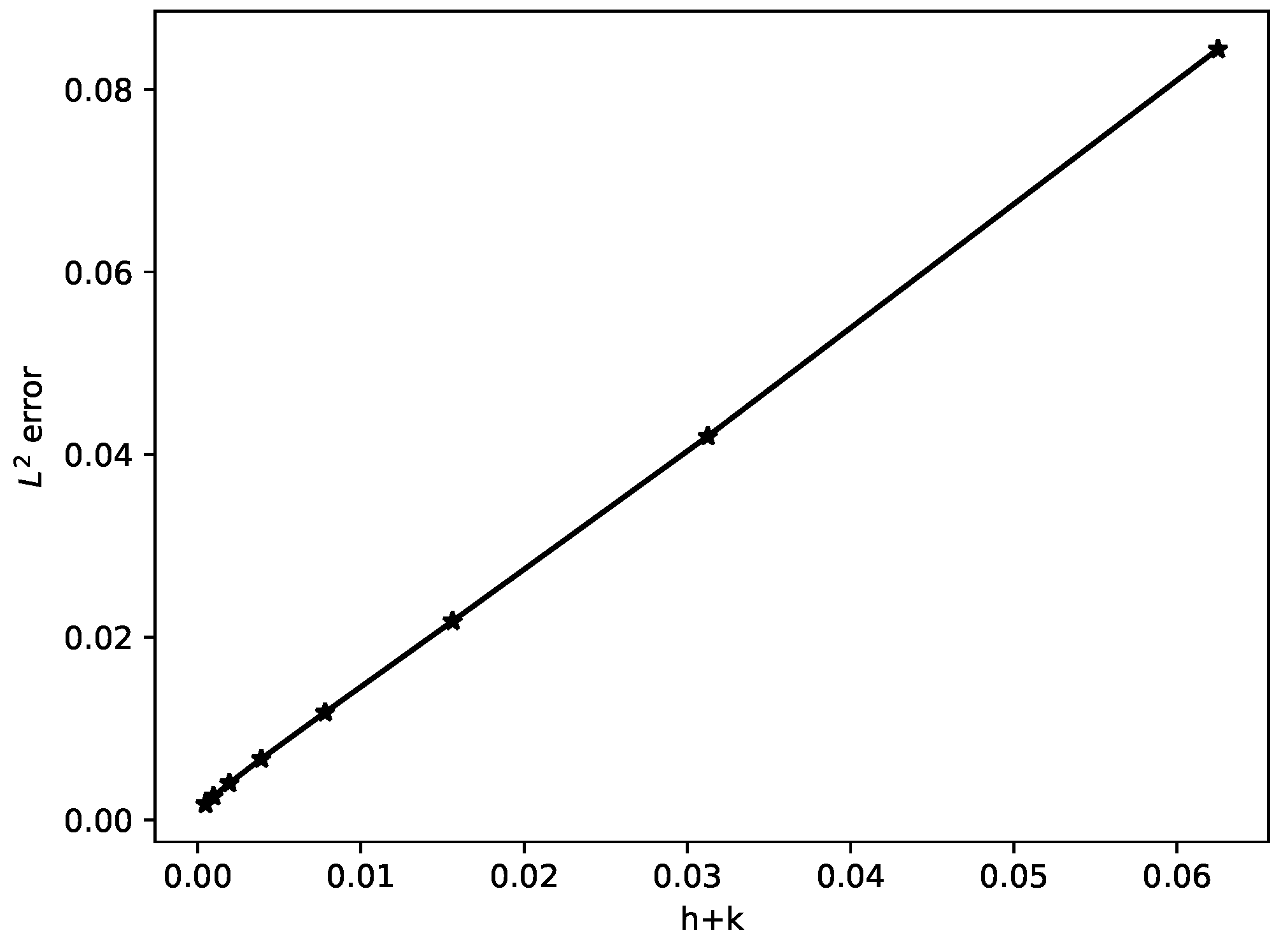
Since the exact solution for the coupled problem is unknown, the solution with a refined mesh ($h=k=3\times {10}^{-5}$) was considered as the reference. The norm of the numerical errors defined in Corollary 1 is shown in

Table 1. Numerical errors ($\times 100$) for some discretizations.

h↓$\mathit{k}\to$	$2^{-5}$	$2^{-6}$	$2^{-7}$	$2^{-8}$	$2^{-9}$	$2^{-10}$	$2^{-11}$	$2^{-12}$	$2^{-13}$
$2^{-5}$	8.440	4.712	2.845	1.925	1.477	1.276	1.202	1.167	1.151
$2^{-6}$	7.919	4.199	2.322	1.387	0.927	0.719	0.644	0.610	0.593
$2^{-7}$	7.768	4.052	2.175	1.236	0.771	0.553	0.474	0.437	0.420
$2^{-8}$	7.707	3.992	2.114	1.175	0.708	0.482	0.400	0.362	0.343
$2^{-9}$	7.668	3.953	2.075	1.135	0.667	0.438	0.348	0.309	0.290
$2^{-10}$	7.634	3.919	2.041	1.100	0.631	0.400	0.301	0.262	0.243
$2^{-11}$	7.602	3.887	2.008	1.067	0.597	0.364	0.256	0.216	0.197
$2^{-12}$	7.570	3.855	1.976	1.034	0.563	0.329	0.214	0.170	0.151
$2^{-13}$	7.539	3.823	1.944	1.001	0.530	0.295	0.178	0.125	0.105

, and the main diagonal of this table is plotted in Figure 1. As we can see, the convergence of the numerical algorithm was found, and the linear convergence, stated in the previous section, seemed to be achieved.

4.3. One-Dimensional Examples

Since, to the best of the authors’ knowledge, there are no one-dimensional examples regarding this model in the literature and they can provide some insights with an easy spatial domain, some examples are shown. The domain represents a horizontal section of the computational domain presented in [27] (the same domain used for the two-dimensional examples in this section); thus, $\Omega =[0,0.6]$. The simulation ran until a final time of one day was reached.

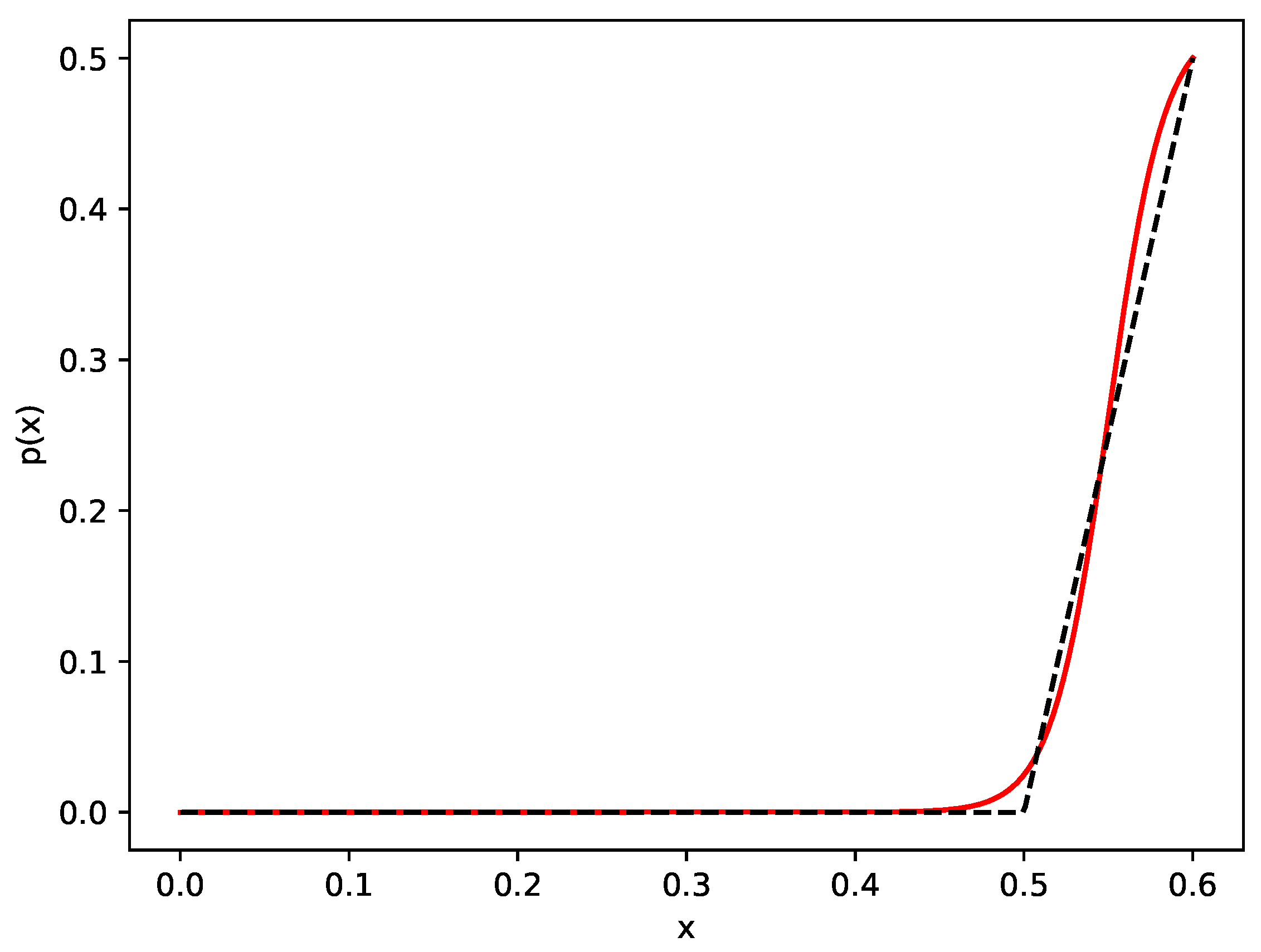
First, we address the definition of function $p\left(x\right)$. As explained in [27], this function must reach its maximum value (which is a model parameter defined as $p_m$ from now on) on the implant surface. Furthermore, it decreases fast to the value of zero (in [27], the function decreases to zero at a distance of 0.1 mm from the implant surface), remaining zero in the rest of the domain. If the support of the function is considered linear, a non-differentiable point appears when the zero value is reached. This could lead to problems since the gradient of this function appears in Equation (1). To avoid problems when the spatial discretization is performed, it is better to create the mesh in such a way that this singular point is not inside an element. This precaution is easy to fulfil in one dimension, but not as easy in a two- or three-dimensional domain.

To address those problems, we propose a different definition of p based on the sigmoid function. It possesses all the properties required for p, while avoiding non-differentiable points. For the one-dimensional example, with a domain of 0.6 mm and a support of 0.1 mm, both graphs are shown in Figure 2, and the definition of p based on the sigmoid results:

$$p\left(x\right)=p_m\frac{1.05}{1+e^{-60(x-0.55)}}\mathrm{for}\mathrm{all}x\in [0,0.6].$$

To show the similar behavior of both approaches, we solve the example with the following parameters:

$$\begin{array}{c}{c}_0=2.5\times {10}^8,m_0=1000,b_0=1000,s_{1_0}=1,s_{2_0}=1,m_{bone}=2\times {10}^5,p_m=0.5,\hfill \\ D_c=0.01638,A_c=1.005,H_c=0.08325,D_m=0.133,B_{m1}=0.667\times {10}^{-2},B_{m2}=0.167,\hfill \\ {\alpha }_{m0}=0.25,{\alpha }_m=0.25,N_m={10}^6,A_m=0.002,{\alpha }_{mb}=0.5,{\beta }_m=10,{\beta }_{mb}=10,\hfill \\ A_b=0.00667,D_{s1}=0.3,D_{s2}=0.1,A_{s1}=10,A_{s2}=10,{\alpha }_{c1}=6.67\times {10}^{-5},\hfill \\ {\alpha }_{c2}={10}^{-5},{\alpha }_{m2}=0.0025,{\alpha }_{b2}=0.0025,{\beta }_{c1}=0.1,{\beta }_{c2}=10,{\beta }_{m2}=10,{\beta }_{b2}=10.\hfill \end{array}$$

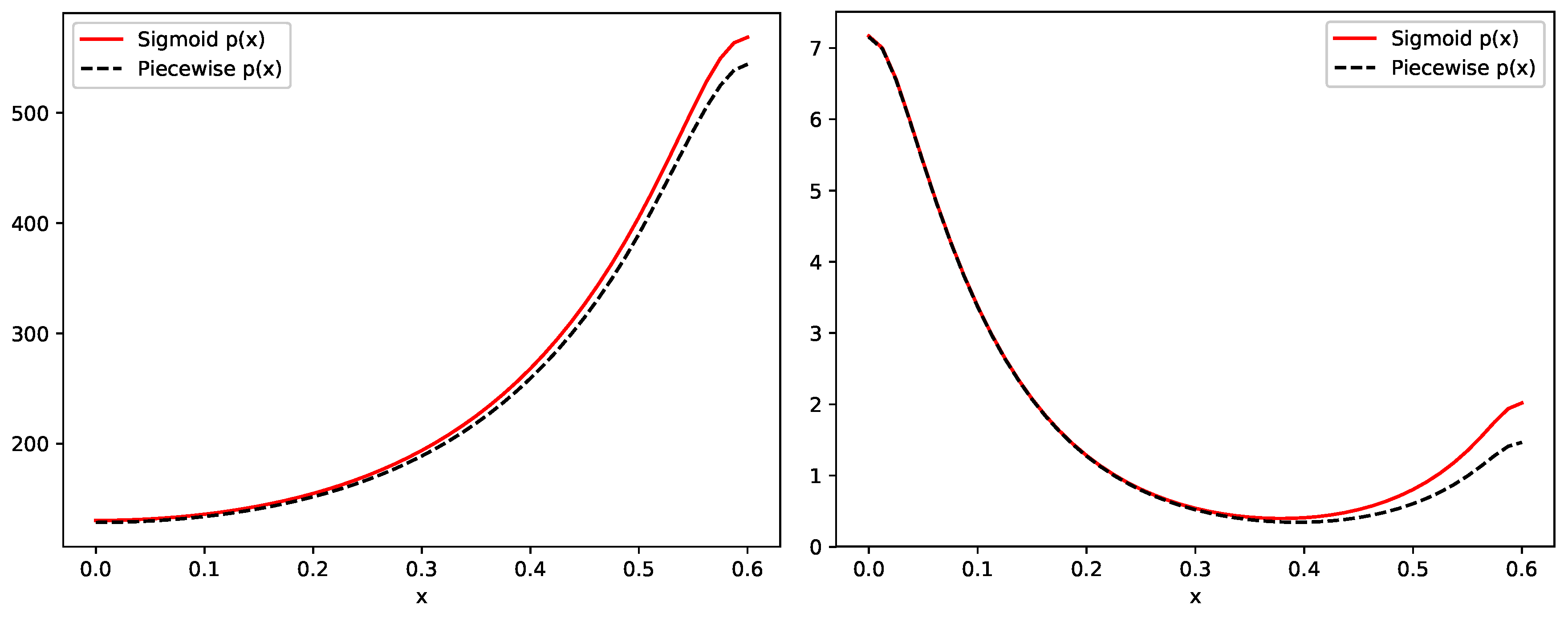
The results for the concentration of platelets (c) and both growth factors ($s_1$ and $s_2$) are shown in Figure 3 and Figure 4, respectively. For the case of platelets, it can be seen that both solutions were qualitatively (and to a great extent, also quantitatively) similar. However, for the case of the piecewise definition of p, a non-differentiable point appeared at $x=0.5$, while in the other case, the solution was smoother. Regarding growth factors, they showed again a similar behavior, slightly differing for values close to $x=0.6$.

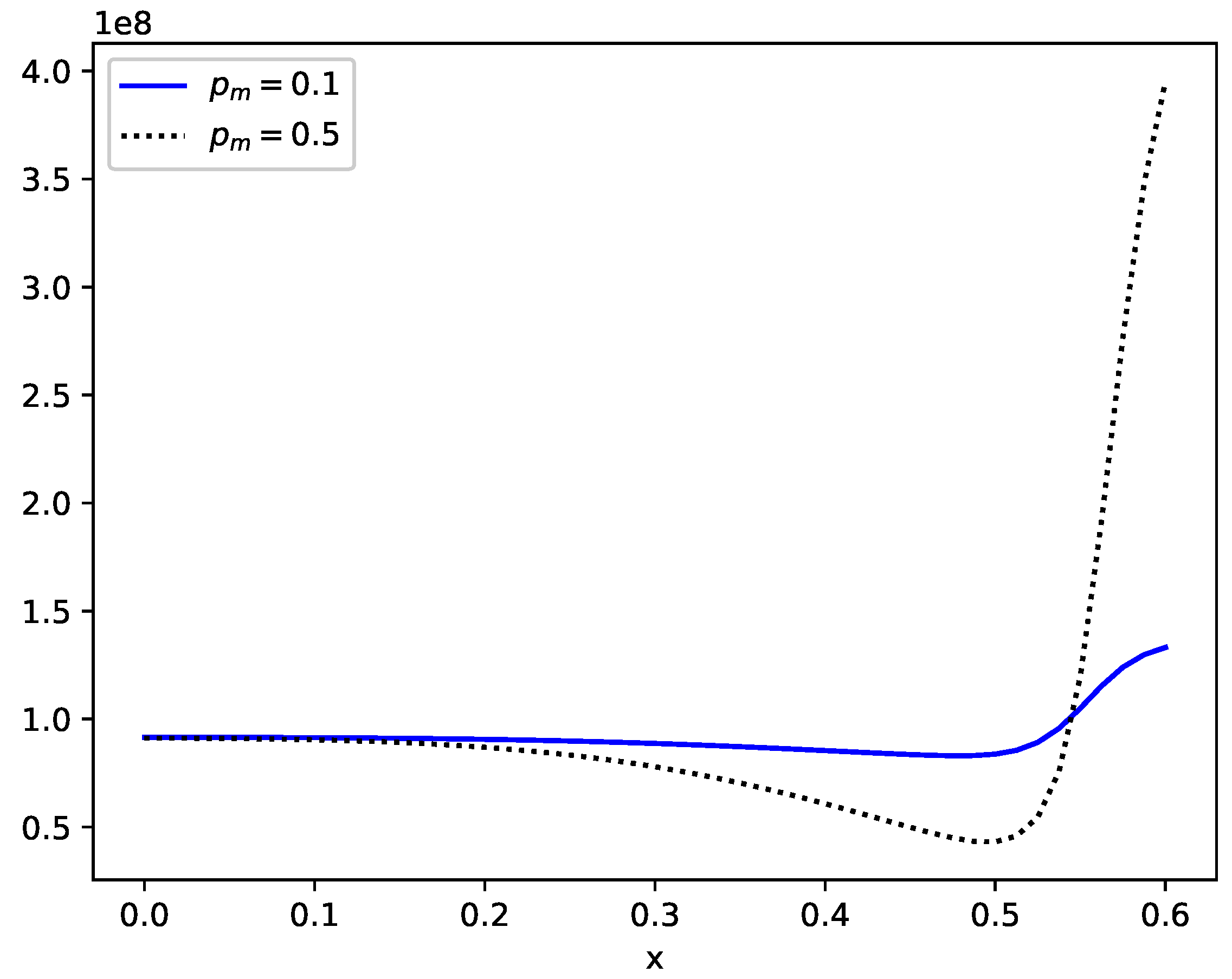
To complete the one-dimensional analysis, we show the difference for the two values of $p_m$, as discussed in [27]. We solved the same problem as before, but now comparing the value for $p_m=0.5$ and $p_m=0.1$. We chose the sigmoid definition for p in this case.

The results for these simulations are shown in Figure 5 (concentration of platelets) and Figure 6 (concentrations of osteogenic cells and osteoblasts). The results showed similar behavior as that found in [27], the shown variables reaching similar values in the left part of the domain (where the values of p were similar) and greatly differing in the right hand side, where the gradient of p was much lower.

4.4. Two-Dimensional Example

We complete the work with an example of the problem in two dimensions. The domain was defined as in [27]. However, due to the symmetry of the problem, only half of the domain was considered. The complete domain and boundaries with the mesh in the lower half are depicted in Figure 7, where the dimensions are shown in millimeters. Function p was defined as a piecewise function in this case, since the extension of the sigmoid function to two dimensions would not solve the non-differentiability where two borders meet (namely, in the bisection of both “implant” borders). To account for this, interior borders were included (only for meshing purposes) in the regions of discontinuity of the gradient of p, thus avoiding singular points inside the elements.

The final time for the simulation was again one day and the parameters for this case were the following:

$$\begin{array}{c}{c}_0=2.5\times {10}^8,m_0=1000,b_0=1000,s_{1_0}=1,s_{2_0}=1,m_{bone}=2\times {10}^5,D_c=0.01638,\hfill \\ A_c=1.005,H_c=0.08325,D_m=0.133,B_{m1}=0.667\times {10}^{-3},B_{m2}=0.167\times {10}^{-2},\hfill \\ {\alpha }_{m0}=0.25,{\alpha }_m=0.25,N_m={10}^6,A_m=0.002,{\alpha }_{mb}=0.5,{\beta }_m=10,{\beta }_{mb}=10,\hfill \\ A_b=0.00667,D_{s1}=0.3,D_{s2}=0.1,A_{s1}=10,A_{s2}=10,{\alpha }_{c2}={10}^{-5},{\beta }_{b2}=10,\hfill \\ {\alpha }_{c1}=6.67\times {10}^{-5},{\alpha }_{m2}=0.0025,{\alpha }_{b2}=0.0025,{\beta }_{c1}=0.1,{\beta }_{c2}=10,{\beta }_{m2}=10.\hfill \end{array}$$

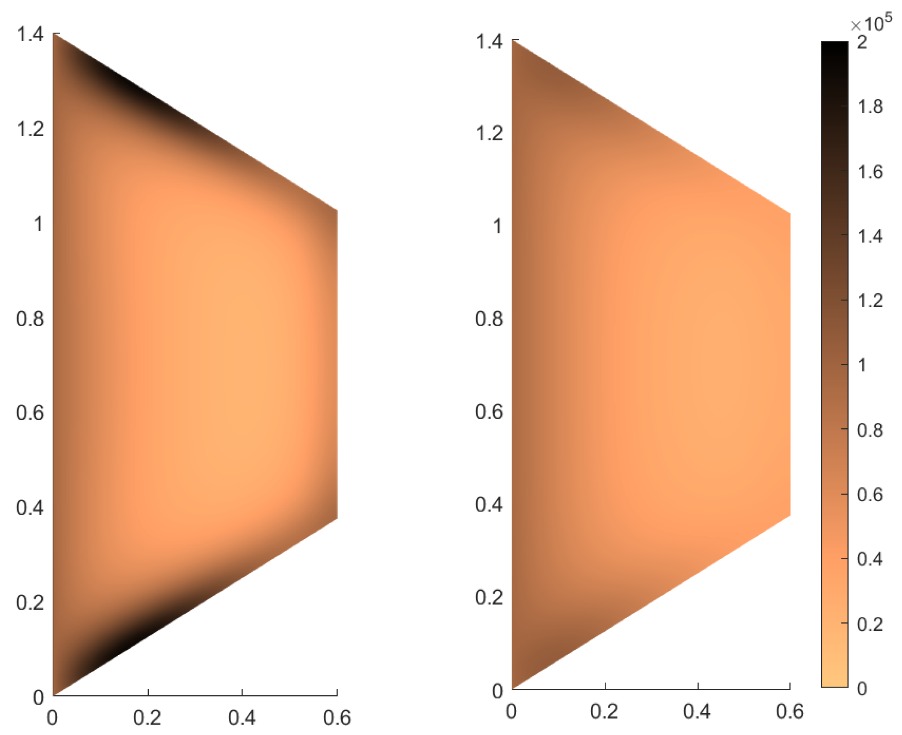
Again, we compared the cases of $p_m=0.1$ and $p_m=0.5$. The obtained results are shown in Figure 8 (platelets density), Figure 9 (osteogenic cell density), and Figure 10 (osteoblasts density). These results agreed qualitatively with published results of the literature and were consistent with the 1D computations.

As in the one-dimensional case, when $p_m=0.1$, the concentration of cells near the implant was much smaller in general. It is also worth noting that for the osteogenic cells (m), the concentrations were higher in the upper and lower implant boundaries than in the right one. This effect also appeared with the osteoblasts, but more accentuated.

5. Conclusions

In this paper, a numerical analysis of a bone remodeling model for endosseous implants was performed. The variational form was obtained, and from that, an algorithm to solve the discrete problem was proposed. The full discretization was done using the well known finite element method and a combination of Euler schemes. This allowed obtaining mathematical results on the convergence of the algorithm. This convergence was exemplified with a one-dimensional simple test example. Some other one-dimensional cases were solved and completed with a two-dimensional solution.

We point out that this work was a first step toward dealing with the study of these osseointegration models. A possible extension could be to consider, for instance, the so-called joint congruence, that is to analyze how the articular surfaces mate each other (see, for instance, [43,44]).

References

- Haas, R.; Polak, C.; Fürhauser, R.; Mailath-Pokorny, G.; Dörtbudak, O.; Watzek, G. A long-term follow-op of 76 Bränemark single-tooth implants. Clin. Oral Implants Res. 2002, 13, 38–43. [Google Scholar] [CrossRef] [PubMed]
- Soncini, M.; Pietrabissa, R.; Rodriguez y Baena, R. Computational approach for the mechanical reliability of a dental implant. In Computer Methods in Biomechanics and Biomedical Engineering; Middleton, J., Pande, G.N., Jones, M.L., Eds.; Gordon and Breach Science Publishers: London, UK, 2001. [Google Scholar]
- Azcarate-Velázquez, F.; Castillo-Oyagüe, R.; Oliveros-López, L.G.; Torres-Lagares, D.; Martínez-González, Á.J.; Pérez-Velasco, A.; Lynch, C.D.; Gutiérrez-Pérez, J.L.; Serrera-Figallo, M.Á. Influence of bone quality on the mechanical interaction between implant and bone: A finite element analysis. J. Dent. 2019, 88, 103–161. [Google Scholar] [CrossRef] [PubMed]
- Baggi, L.; Cappelloni, I.; Di Girolamo, M.; Maceri, F.; Vairo, G. The influence of implant diameter and length on stress distribution of osseointegrated implants related to crestal bone geometry: A three-dimensional finite element analysis. J. Prosthet. Dent. 2008, 100, 422–431. [Google Scholar] [CrossRef] [Green Version]
- Cos Juez, F.J.; Sánchez Lasheras, F.; García Nieto, P.G.; Álvarez-Arenal, A. Non-linear numerical analysis of a double-threaded titanium alloy dental implant by FEM. Appl. Math. Comput. 2008, 2008, 952–967. [Google Scholar] [CrossRef]
- Dorogoy, A.; Haïat, G.; Shemtov-Yona, K.; Rittel, D. Modeling ultrasonic wave propagation in a dental implant—Bone system. J. Mech. Behav. Biomed. Mater. 2019, 20, 103. [Google Scholar] [CrossRef]
- Farronato, D.; Manfredini, M.; Stevanello, A.; Campana, V.; Azzi, L.; Farronato, M. A Comparative 3D Finite Element Computational Study of Three Connections. Materials 2019, 12, 3135. [Google Scholar] [CrossRef] [Green Version]
- Fernandez, J.W.; Das, R.; Cleary, P.W.; Hunter, P.J.; Thomas, C.D.L.; Clement, J.G. Using smooth particle hydrodynamics to investigate femoral cortical bone remodeling at the Haversian level. Int. J. Numer. Methods Biomed. Eng. 2013, 29, 129–143. [Google Scholar] [CrossRef]
- Giorgio, I.; Andreaus, U.; Scerrato, D.; Braidotti, P. Modeling of a non-local stimulus for bone remodeling process under cyclic load: Application to a dental implant using a bioresorbable porous material. Math. Mech. Solids 2017, 22, 1790–1805. [Google Scholar] [CrossRef] [Green Version]
- Guan, H.; van Staden, R.C.; Johnson, N.; Loo, Y.-C. Dynamic modeling and simulation of dental implant insertion process—A finite element study. Finite Elem. Anal. Des. 2011, 47, 886–897. [Google Scholar] [CrossRef] [Green Version]
- Hasan, I.; Rahimi, A.; Keilig, L.; Brinkmann, K.T.; Bourauel, C. Computational simulation of internal bone remodeling around dental implants: A sensitivity analysis. Comput. Methods Biomech. Biomed. Eng. 2012, 15, 807–814. [Google Scholar] [CrossRef]
- He, Y.; Hasan, I.; Keilig, L.; Fischer, D.; Ziegler, L.; Abboud, M.; Wahl, G.; Bourauel, C. Biomechanical characteristics of immediately loaded and osseointegration dental implants inserted into Sika deer antler. Med. Eng. Phys. 2018, 59, 8–14. [Google Scholar] [CrossRef] [PubMed]
- He, Y.; Hasan, I.; Keilig, L.; Fischer, D.; Ziegler, L.; Abboud, M.; Wahl, G.; Bourauel, C. Numerical investigation of bone remodeling around immediately loaded dental implants using sika deer (Cervus nippon) antlers as implant bed. Comput. Methods Biomech. Biomed. Eng. 2018, 21, 359–369. [Google Scholar] [CrossRef] [PubMed]
- Hoang, K.C.; Khoo, B.C.; Liu, G.R.; Nguyen, N.C.; Patera, A.T. Rapid identification of material properties of the interface tissue in dental implant systems using reduced basis method. Inverse Probl. Sci. Eng. 2013, 21, 1310–1334. [Google Scholar] [CrossRef]
- Hou, P.J.; Ou, K.L.; Wang, C.C.; Huang, C.F.; Ruslin, M.; Sugiatno, E.; Yang, T.S.; Chou, H.H. Hybrid micro/nanostructural surface offering improved stress distribution and enhanced osseointegration properties of the biomedical titanium implant. J. Mech. Behav. Biomed. Mater. 2018, 79, 173–180. [Google Scholar] [CrossRef]
- Joshi, S.; Kumar, S.; Jain, S.; Aggarwal, R.; Choudhary, S.; Reddy, N.K. 3D Finite Element Analysis to Assess the Stress Distribution Pattern in Mandibular Implant-supported Overdenture with Different Bar Heights. J. Contemp. Dent. Pract. 2019, 20, 794–800. [Google Scholar] [CrossRef] [PubMed]
- Kurniawan, D.; Nor, F.M.; Lee, H.Y.; Lim, J.Y. Finite element analysis of bone-implant biomechanics: Refinement through featuring various osseointegration conditions. Int. J. Oral Maxillofac. Surg. 2012, 41, 1090–1196. [Google Scholar] [CrossRef] [PubMed]
- Lencioni, K.A.; Noritomi, P.Y.; Macedo, A.P.; Ribeiro, R.F.; Almeida, R.P. Influence of different implants on the biomechanical behavior of tooth-implant fixed partial dentures: A three-dimensional finite element analysis. J. Oral Implantol. 2019. [Google Scholar] [CrossRef]
- Lima de Andrade, C.; Carvalho, M.A.; Bordin, D.; da Silva, W.J.; del Bel Cury, A.A.; Sotto-Maior, B.S. Biomechanical Behavior of the Dental Implant Macrodesign. Int. J. Oral Maxillofac. Implant. 2017, 32, 264–270. [Google Scholar] [CrossRef] [Green Version]
- Lin, D.; Li, Q.; Li, W.; Duckmanton, N.; Swain, M. Mandibular bone remodeling induced by dental implant. J. Biomech. 2010, 43, 287–293. [Google Scholar] [CrossRef]
- Murase, K.; Stenlund, P.; Thomsen, P.; Lausmaa, J.; Palmquist, A. Three-dimensional modeling of removal torque and fracture progression around implants. J. Mater. Sci. Mater. Med. 2018, 29, 104. [Google Scholar] [CrossRef] [Green Version]
- Rittel, D.; Dorogoy, A.; Shemtov-Yona, K. Modeling the effect of osseointegration on dental implant pullout and torque removal tests. Clin. Implant Dent. Relat. Res. 2018, 20, 683–691. [Google Scholar] [CrossRef] [PubMed]
- Sayyedi, A.; Rashidpour, M.; Fayyaz, A.; Ahmadian, N.; Dehghan, M.; Faghani, F.; Fasihg, P.J. Comparison of Stress Distribution in Alveolar Bone with Different Implant Diameters and Vertical Cantilever Length via the Finite Element Method. Long Term Eff. Med. Implant. 2019, 29, 37–43. [Google Scholar] [CrossRef]
- Sotto-Maior, B.S.; Mercuri, E.G.; Senna, P.M.; Assis, N.M.; Francischone, C.E.; del Bel Cury, A.A. Evaluation of bone remodeling around single dental implants of different lengths: A mechanobiological numerical simulation and validation using clinical data. Comput. Methods Biomech. Biomed. Eng. 2016, 19, 699–706. [Google Scholar] [CrossRef] [PubMed]
- Wang, C.; Li, Q.; McClean, C.; Fan, Y. Numerical simulation of dental bone remodeling induced by implant- supported fixed partial denture with or without cantilever extension. Int. J. Numer. Method Biomed. Eng. 2013, 29, 1134–1147. [Google Scholar] [CrossRef] [PubMed]
- Zheng, L.; Yang, J.; Hu, X.; Luo, J. Three dimensional finite element analysis of a novel osteointegrated dental implant designed to reduce stress peak of cortical bone. Acta Bioeng. Biomech. 2014, 16, 21–28. [Google Scholar] [PubMed]
- Moreo, P.; García-Aznar, J.M.; Doblaré, M. Bone ingrowth on the surface of endosseous implants. Part 1: Mathematical model. J. Theor. Biol. 2009, 260, 1–12. [Google Scholar] [CrossRef] [Green Version]
- Moreo, P.; García-Aznar, J.M.; Doblaré, M. Bone ingrowth on the surface of endosseous implants. Part 2: Theoretical and numerical analysis. J. Theor. Biol. 2009, 260, 13–26. [Google Scholar] [CrossRef] [Green Version]
- Fernández, J.R.; García-Aznar, J.M.; Masid, M. Numerical analysis of an osteoconduction model arising in bone-implant integration. ZAMM Z. Angew. Math. Mech. 2017, 97, 1050–1063. [Google Scholar]
- Fernández, J.R.; Masid, M. Analysis of a model for the propagation of the ossification front. J. Comput. Appl. Math. 2017, 318, 624–633. [Google Scholar]
- Lekszycki, T.; dell’Isola, F. A mixture model with evolving mass densities for describing synthesis and resorption phenomena in bones reconstructed with bio-resorbable materials. Zeit. Ang. Math. Mech. 2012, 92, 426–444. [Google Scholar] [CrossRef] [Green Version]
- Lu, Y.; Lekszycki, T. New description of gradual substitution of graft by bone tissue including biomechanical and structural effects, nutrients supply and consumption. Cont. Mech. Thermod. 2018, 30, 995–1009. [Google Scholar] [CrossRef] [Green Version]
- George, D.; Allena, R.; Rémond, Y. Integrating molecular and cellular kinetics into a coupled continuum mechanobiological stimulus for bone reconstruction. Cont. Mech. Thermod. 2019, 31, 725–740. [Google Scholar] [CrossRef] [Green Version]
- Barbu, V. Optimal Control of Variational Inequalities; Pitman: Boston, MA, USA, 1984. [Google Scholar]
- Brezis, H. Equations et inéquations non linéaires dans les espaces vectoriels en dualité. Ann. Inst. Fourier 1968, 18, 115–175. [Google Scholar] [CrossRef] [Green Version]
- Chau, O.; Fernández, J.R.; Shillor, M.; Sofonea, M. Variational and numerical analysis of a quasistatic viscoelastic contact problem with adhesion. J. Comput. Appl. Math. 2003, 159, 431–465. [Google Scholar] [CrossRef] [Green Version]
- Ciarlet, P.G. Basic error estimates for elliptic problems. In Handbook of Numerical Analysis; Ciarlet, P.G., Lions, J.L., Eds.; 1993; Volume II, pp. 17–351. [Google Scholar]
- Barboteu, M.; Fernández, J.R.; Hoarau-Mantel, T.V. A class of evolutionary variational inequalities with applications in viscoelasticity. Math. Model. Methods Appl. Sci. 2005, 15, 1595–1617. [Google Scholar] [CrossRef]
- Campo, M.; Fernández, J.R.; Kuttler, K.L.; Shillor, M.; Viaño, J.M. Numerical analysis and simulations of a dynamic frictionless contact problem with damage. Comput. Methods Appl. Mech. Eng. 2006, 196, 476–488. [Google Scholar] [CrossRef]
- Alnaes, S.; Blechta, J.; Hake, J.; Johansson, A.; Kehlet, B.; Logg, A.; Richardson, C.; Ring, J.; Rognes, M.E.; Wells, G.N. The FEniCS Project Version 1.5 M. Arch. Numer. Softw. 2005, 3. [Google Scholar] [CrossRef]
- Logg, A.; Mardal, K.-A.; Wells, G.N. (Eds.) Automated Solution of Differential Equations by the Finite Element Method; Springer: Berlin/Heidelberg, Germany, 2012. [Google Scholar]
- Hecht, F. New development in FreeFem++. J. Numer. Math. 2012, 20, 251–265. [Google Scholar] [CrossRef]
- Conconi, M.; Parenti-Castelli, V. A sound and efficient measure of joint congruence. Proc. Inst. Mech. Eng. Part H J. Eng. Med. 2014, 228, 935–941. [Google Scholar] [CrossRef]
- Valigi, M.C.; Logozzo, S. Do Exostoses Correlate with Contact Disfunctions? A Case Study of a Maxillary Exostosis. Lubricants 2019, 7, 15. [Google Scholar] [CrossRef] [Green Version]
Figure 1.
Asymptotic linear convergence.
Figure 2.
Graph of p defined as a sigmoid (red) and the piecewise form (dashed black), for .
Figure 3.
Concentration of platelets along the spatial domain at the final time.
Figure 4.
Concentration of growth factors (left) and (right) at the final time.
Figure 5.
Concentration of platelets along the spatial domain at the final time for the case of (blue) and (black).
Figure 6.
Concentration of osteogenic cells (left) and osteoblasts (right) at the final time for the case of (blue) and (black).
Figure 7.
Computational domain and mesh for the two-dimensional problem. Due to the symmetry of the problem, only half of the domain was simulated. Interior borders were added to ensure that at the regions of discontinuity for the derivatives of p, only edges were placed. Dimensions in mm.
Figure 8.
Concentration of platelets at the final time for the case of (left) and (right).
Figure 9.
Concentration of osteogenic cells at the final time for the case of (left) and (right).
Figure 10.
Concentration of osteoblasts at the final time for the case of (left) and (right).