Exchange Market Liquidity Prediction with the K-Nearest Neighbor Approach: Crypto vs. Fiat Currencies


1
Universidad Autonoma de Nuevo Leon, Facultad de Contaduria Publica y Administracion, San Nicolás de los Garza 66451, Mexico
2
Tecnologico de Monterrey, EGADE Business School, San Pedro Garza García 66269, Mexico
3
Universidad del Pacífico, Departamento de Finanzas, Jesús María 15072, Peru
*
Author to whom correspondence should be addressed.
Mathematics 2021, 9(1), 56; https://doi.org/10.3390/math9010056
Submission received: 17 November 2020
/
Revised: 11 December 2020
/
Accepted: 23 December 2020
/
Published: 29 December 2020
(This article belongs to the Special Issue Mathematics of Financial Operations)
Abstract
:In this paper, we compare the predictions on the market liquidity in crypto and fiat currencies between two traditional time series methods, the autoregressive moving average (ARMA) and the generalized autoregressive conditional heteroskedasticity (GARCH), and the machine learning algorithm called the k-nearest neighbor (KNN) approach. We measure market liquidity as the log rates of bid-ask spreads in a sample of three cryptocurrencies (Bitcoin, Ethereum, and Ripple) and 16 major fiat currencies from 9 February 2018 to 8 February 2019. We find that the KNN approach is better suited for capturing the market liquidity in a cryptocurrency in the short-term than the ARMA and GARCH models maybe due to the complexity of the microstructure of the market. Considering traditional time series models, we find that ARMA models perform well when estimating the liquidity of fiat currencies in developed markets, whereas GARCH models do the same for fiat currencies in emerging markets. Nevertheless, our results show that the KNN approach can better predict the log rates of the bid-ask spreads of crypto and fiat currencies than ARMA and GARCH models.
1. Introduction
The popularity of cryptocurrency with financial intermediaries came about as a consequence of the perceived failures of the monetary authorities in the global financial crisis of 2008 and the European sovereign debt crisis during 2010 to 2013 [1]. In terms of monetary attributes, Yermack [2] explains that Bitcoin does not behave similarly to a fiat currency according to the criteria widely used by economists. For instance, some economists view the inelasticity in the supply of cryptocurrency as an advantage but some view it as a disadvantage.
Cryptocurrencies are digital coins not issued by any government or legal entity [3]; they only use cryptography and a clever system to regulate their supply, control trading operations and avoid frauds. The transactions are recorded digitally in a blockchain as an accounting system [4]. Digital currencies are based on peer-to-peer authentication with rules to determine the amount and condition produced [5]. These currencies plan the peer-to-peer network as a set of nodes in a self-organizing connected network. Hayes [6] has identified that the relative differences in the cost of mining on the margin determine the prices of cryptocurrencies. The most popular cryptocurrency is Bitcoin, which was developed in the seminal paper of Nakamoto [7]. Bitcoin, Ethereum, and Ripple are the main cryptocurrencies capitalized by the market as reported by Blas [8].
Conversely, Dwyer [5] reports that governments create and certify fiat currencies that are used by all. In terms of networks, this is similar to a client–server model in which one server receives requests from clients and responds to them. The server ensures the data precision of whatever information it provides. The issuer designs a fiat currency to hinder counterfeiting and enforces laws that make counterfeiting a crime.
What are the most important challenges in the cryptocurrency market? Encrybit [9], a cryptocurrency exchange platform, conducted a survey among 1108 traders between 23 April and 30 April 2018 and identified the three biggest problems in the cryptocurrency market: lack of security (40%), high trading fees (37%), and lack of liquidity (36%). The first problem deals with more sophisticated hackers who endanger the exchange platforms. The second problem arises because many exchanges split their trading fees into two separate fees in which the maker fee is higher than the taker fee because the former adds liquidity to the market. The third problem is price manipulation and high volatility in which brokers do not place orders or execute them on time.
Crook [10] argues that the illiquidity problem needs to be solved in order to democratize access to the cryptocurrency market, make it more efficient, and avoid perverse incentives from the different players. Jiang et al. [11] make a bibliometric research of 918 papers published between 2009 and 2019 about the cryptocurrency market and conclude that there was a shift in the main topic from technological to economic. Furthermore, the most important economic topic is explaining and forecasting the volatility in the cryptocurrency market. The most common statistical models that studies use to explain or predict market volatility are parametric such as the GARCH-type family.
The literature related to the liquidity of the cryptocurrency market is even more recent than the literature related to its volatility and has different strands: market microstructure explanations [12], the relation between liquidity and volatility [13,14], the factors that affect market liquidity [15,16], and how to measure liquidity in the cryptocurrency market [17].
None of the above strands have tried to explain or predict the liquidity in the cryptocurrency market. Furthermore, given the microstructure complexity of this liquidity, we assert that the use of nonparametric models would be better for predicting it. In this sense, we find that the k-nearest neighbor (KNN) approach, which is a supervised machine learning algorithm, is better suited to predict the liquidity of the cryptocurrency market than a classical linear model such as the autoregressive moving average (ARMA) model or a nonlinear model such as the generalized autoregressive conditional heteroskedasticity (GARCH) that are intensively used to predict volatility.
Although there have been several investors’ clampdown events on cryptocurrency trading due to market news, these pieces of news are later incorporated into prices due to the short-term memory of Bitcoin returns that exhibit short term momentum and reversals [18]. It is important to clarify that the mechanism through which news may be added into cryptocurrency prices is short-term for cryptocurrencies’ returns, but long-term for cryptocurrencies returns’ volatility. Nevertheless, liquidity is at the bottom of the explanation.
Khuntia and Pattanayak [19] present an event history in the Bitcoin market from January 2015–June 2018 and suggest that these events impact the trading volume and the long-memory in volatility of bitcoin returns. Furthermore, Phillip et al. [20] found that slower transacted cryptocurrencies, such as Bitcoin, have less long memory, whereas faster transacted coins, such as Ripple display more long memory. In other words, the day-to-day volatility correlation (long memory in return volatility) is dependent on completion times and therefore liquidity.
Thus, the main objective of this study is to determine the best model for predicting the short-term log rates of the bid-ask spreads in the three biggest cryptocurrencies—Bitcoin, Ripple, and Ethereum—and in the 16 major fiat currencies listed by Bloomberg. Consequently, our research question is the following: Is the KNN approach a better predictor of the short-term liquidity of cryptocurrencies than classical time-series models? To the best of our knowledge, there is no other study that has addressed this question, and given the importance of market liquidity, we argue that it is necessary to find better ways to assess the liquidity of the cryptocurrency market (long-term memory in the cryptocurrency market liquidity is beyond the scope of our study).
2. Literature Review
According to Jiang et al. [11], the research trend of the last decade in the published papers related to cryptocurrency has changed from a technological perspective to an economic one. Specifically, their focus has been to try to explain the volatility of cryptocurrencies with traditional statistical models such as generalized autoregressive conditional heteroskedasticity model (GARCH) and its derivations.
Financial time series, as Ruppert [21] mentions, often exhibit volatility clustering in assets returns, where periods of high volatility and periods of low volatility could be present, i.e., time-varying volatility is more common than constant volatility. In this sense, Nelson [22] comments that GARCH models elegantly capture the volatility and this feature accounts for both their theoretical appeal and their empirical success. Thus, as Venter and Maré [23] argue, the GARCH model has become increasingly popular among both academics and practitioners for modelling time-varying volatility in financial time series analysis, including cryptocurrencies.
GARCH-type models are actually used not only for examining mean returns but also a volatility return transmission within the VAR-GARCH model; for example, Loverta and Lopez [24] focus on credit default swap (CDS) spreads as a directly observable market indicator of default risk within the VAR-BEKK-GARCH framework.
Kyriazis et al. [25] study the volatility of the three most highly capitalized digital currencies (Bitcoin, Ethereum, and Ripple) during a bearish market and find that during distressed times, no possibilities for hedging exist between the majority of cryptocurrencies and the three major ones. Walther et al. [26] use the GARCH-MIDAS framework to identify drivers of cryptocurrency volatility and find that the global real economic activity provides superior volatility predictions for both bull and bear markets. Acereda et al. [27] study the expected shortfall of the main cryptocurrencies and find that the best results come from using a NGARCH.
Fakhfekh and Jeribi [28] model the volatility of 16 cryptocurrencies and find that the TGARCH was the best specification, whereas Cerqueti et al. [29] find that relaxing the normality assumption and considering skewed distributions, such as a skewed non-Gaussian GARCH models, yield better predictions for the cryptocurrencies’ volatility. One of the most comprehensive studies about the usefulness of GARCH-type models for forecasting Bitcoin’s volatility is the one by Köchling et al. [30]. Interestingly, the authors find that most GARCH-type models have equal predictive ability and that some specifications are outperformed on a regular basis.
In the last two years, several authors have focused their attention on cryptocurrencies’ liquidity. Stenfors [31] defines the bid-ask spread as a bonus that is paid to market makers for standing ready to absorb the risk borne by others “immediately” and that the spread is closely connected to market liquidity. For the case of fiat exchange rate markets, Stenfors [31] uses the spread as a proxy, whereas Dyhrberg et al. [12] use it for the case of cryptocurrency markets. Kim [32] finds that Bitcoin markets have bid-ask spreads that are approximately 2% lower than the main fiat currencies due to lower transaction costs.
Furthermore, there is a strong relation between the volatility and liquidity of the cryptocurrency market. Wei [13] shows that volatility decreases as liquidity increases in cryptocurrencies and that there is no sign of an illiquidity premium. Będowska-Sójka et al. [14] obtain a contrasting result in that high volatility in the cryptocurrency market attracts new investors and that this attraction causes an increase in the market liquidity. Brauneis et al. [15] and Scharnowski [16] show that the liquidity of cryptocurrencies depends specifically on the volatility of their returns, the dollar trading volume, and the number of transactions and that general financial market variables have no influence. Brauneis et al. [15] show that a universal best measure for the liquidity of cryptocurrencies does not exist yet because it depends on the application.
There is also research related to the long-term memory of cryptocurrencies returns’ volatility, where the long memory describes the high order correlation structure of a series. Fakhfekha and Jeribi [28] studied sixteen of the most popular cryptocurrencies with five GARCH-type models to predict long-term memory in cryptocurrencies returns’ volatility and found the TGARCH with double exponential distribution to be the best model.
Lahmiri et al. [33] studied the nonlinear patterns of volatility in seven Bitcoin markets. They investigate the fractional long-range dependence in conjunction with the potential inherent stochasticity of volatility time series under four diverse distributional assumptions and found the existence of long memory in Bitcoin market volatility, irrespectively of distributional inference. Hence, in explaining long memory in cryptocurrencies returns’ volatility it is useful to consider Markov-Switching Multifractal Models (MSM) or a sort of hybrid model between pure parametric models and non-parametric ones, such as the Fractionally Integrated GARCH model.
Finally, research has shifted towards non-parametric models to forecast cryptocurrencies returns’ volatility. Khaldi et al. [34] compared different type-GARCH models and Artificial Neural Networks (ANN) models in an attempt to forecast the Bitcoin returns’ volatility. They found that a type of ANN (the Multilayer Perceptron-MLP) outperformed all the parametric and nonparametric models, but it was only effective in short-term forecasting.
The previous review clearly finds that the most important economic concern in the cryptocurrency market has been its volatility, but now the focus is starting to shift to its liquidity. Nevertheless, so far there has been no attempt to predict this short-term liquidity. Furthermore, there is no consensus on what the best method is for predicting the market volatility (beyond a type of hybrid or a non-parametric model), nor what the best measure is for predicting liquidity, but it is possible to use the bid-ask spread as a measure of liquidity and a non-parametric model. Moreover, although there is a strong relation between volatility and liquidity, there is no consensus on the direction of the relation or whether all factors that affect this relation are within the market network.
3. Methodology
3.1. Data and Hypothesis
The study is motived by empirical evidence based on the idea that even though cryptocurrencies exhibit similar features of fiat currencies their market structure is fundamentally different, as is noted by Dyhrberg et al. [12]. Furthermore, Saadah and Whafa [35] pointed out that cryptocurrencies are the most fluctuating product on the market and their high volatility makes liquidity prediction difficult. Therefore, modeling cryptocurrency prediction using classical time series methods coupled with the scarcity of a reliable data source could be a challenge. In this sense, KNN algorithm has been applied as a fundamental prediction technique when there is little or no prior knowledge about the distribution of the data [36]. Due to the complexity of the market microstructure in crypto and fiat currencies, we test whether nonparametric machine learning, such as the KNN approach, is better suited for predicting short-term liquidity in the cryptocurrency market rather than parametric time-series models that studies have widely used to predict volatility. Hence, we propose the following hypothesis based on Gandal and Halaburda [4], Stenfors [31], Kim [32], and Katsiampa [37].
Hypothesis 1.
The nonparametric KNN approach is a better method to predict the short-term liquidity of crypto and fiat currencies than classical ARMA and GARCH models.
The data are the log rates of the daily closing bid-ask spreads from 9 February 2018 to 8 February 2019, for a total of 259 observations for each of the 19 currencies in the study. The log rates were calculated by taking the logarithm of the USD price ratio of the spreads for each currency.
The sample comprises three cryptocurrencies (Bitcoin, Ethereum, and Ripple) and 16 major fiat currencies: the Australian dollar, Brazilian real, British pound, Canadian dollar, Danish krone, euro, Japanese yen, Mexican peso, New Zealand dollar, Norwegian krone, Singaporean dollar, South African rand, South Korean won, Swedish krona, Swiss franc, and Taiwanese dollar. The data are publicly available on the Bloomberg database.
3.2. ARMA and GARCH Models
First, we used the augmented Dickey–Fuller (ADF) statistic to test for the presence of a unit root to rigorously verify the nonstationary nature of the log rates of the bid-ask spreads, with . If the null hypothesis of the presence of a unit root is rejected, then the stationarity autoregressive is guaranteed at least in the mean [38].
Once we applied the ADF test, we continued to analyze the ARMA model proposed by Box and Jenkins [39]. The generalized ARMA(p,q) model that includes both the p-autoregressive and the q-moving average terms is represented as follows:
where and are the parameters for the autoregressive and moving average models, respectively, such as and ; is the delay operator, and the value of its exponent indicates the order of the delay that means ; is the constant parameter; and is the residuals with .
We used the Schwarz criterion (SC) developed by Schwarz [40] that penalizes the inclusion of a greater number of parameters compared with the Akaike Information Criterion (AIC) proposed by Akaike [41] and therefore avoids errors in the estimation of models with large numbers of parameters. For ARMA models, Koehler and Murphree [42] confirms in an empirical study that the SC is a better criterion than AIC and validates the results of others that the AIC will overfit the data. To select the best ARMA(p,q), we used the model with the lowest SC. Second, we applied the GARCH(p,q) model proposed by Bollerslev [43] that considers the dependence of the conditional variance () on the past squared residuals of the model () and the past values of the variance () for the time series. In this context, the modeling of the conditional mean and conditional variance is governed by the following:
where is the time delay parameter of the squared residuals; is the time delay parameter of the past values of the variance; , with and with are the estimated coefficients; and represents the standardized residuals with . To select the parameters , we also applied the SC, which has been shown to exhibit a higher degree of accuracy in identifying the true data generating process than AIC [44].
3.3. Nearest Neighbor Method
Fix and Hodges [45] introduced the nearest neighbor rule as a non-parametric method for pattern classification. Later, Cover and Hart [46] formalized mathematically the method. As a nonparametric method, in the KNN algorithm no explicit assumptions about the underlying data distribution are needed. The KNN besides a classification tool is also used as forecasting technique that considers the spatial correlation between the points of a phase space to improve short-term prediction.
Bajo-Rubio et al. [47] apply the KNN to the foreign exchange market to indicate the potential utility not only as a tool for the prediction of the daily exchange rate but also for the rules of purchase or sales in the technical analysis. Fernández-Rodríguez et al. [48] state that the basic idea behind these predictors is that pieces of the time series in the past might resemble pieces in the future.
The KNN algorithm used in this study can be explained following the next steps from Finkenstädt and Kuhbier [49], and Arroyo and Maté [50]:
- (1)
- The time series considered, , is transformed into a series of -dimensional vectors:where , with being the number of lags and being the delay parameter. In the KNN forecasting algorithm, and are pre-determined parameters.
- (2)
- To simplify, we shall only consider the case of , then the resulting time series of vectors is denoted by , with , which represents a vector of consecutive observations that can be characterized as a point in -dimensional space:These -dimensional vectors are often called -histories, whereas the -dimensional space is referred to as the phase space of time series.
- (3)
- The distance between the last vector, also called focal, and each vector in the time series with is computed. The distance used in this study is the sum over all dimensions of the absolute difference between the values of the cases ( and with ) also called the Manhattan distance or city block metric.
- (4)
- The vector closest to is selected and denoted by . The parameter is also pre-determined using a criteria selection, generally the with the lowest sum of squares residuals (SSRs).
- (5)
- Given the neighboring vectors ; their subsequent values, , are averaged to obtain the forecast, .
Thus, the KNN searches for segments with similar dynamic behavior and uses them to produce the forecast. In this sense, the future short-term evolution of the time series will then be calculated using the historical patterns. To compare the above time-series methods and select the best model, we calculated the average of the sum-of-squares residual (SSR) for the ARMA, GARCH, and KNN methods. The selected model had the lowest SSR.
4. Results
4.1. Descriptive Statistics
Table 1 lists the main descriptive statistics of the depreciation rates of crypto and fiat currencies. Practically all currencies appreciate versus the USD during the time span considered in this study, but the greatest appreciations occur for the cryptocurrencies. The highest kurtosis and volatility values are quantified in the cryptocurrencies and emerging market currencies, such as the Brazilian real and Mexican peso.
However, if we consider the log rates of the bid-ask spreads (see Table 2), the results are mixed. Bitcoin and the main emerging currencies have lower log rates and volatilities than Ripple and Ethereum, but all the cryptocurrencies of the sample are situated in the lowest kurtosis values, which indicate fewer outliers.
4.2. ARMA Models
Table 3 presents the ADF test. This test rejects the null hypothesis of the presence of unit roots in all cases, which means the series is stationary, at least for the mean; thus, the ARMA models can be applied. The research generally uses the Ljung–Box test to validate the ARMA models. This test can confirm the null hypothesis that the residuals of the model do not present a linear correlation. However, it does not allow for a distinction between random and nonlinear dependence. Therefore, we consider the Brock, Dechert, and Scheinkman (BDS) test to detect the presence of nonlinear dependence [51].
Eight currencies could be estimated through a linear stochastic model such as the ARMA, as there was no evidence to reject the hypothesis that the residuals of the model are an independently and identically distributed (iid) series: Canadian dollar, British pound, euro, South African rand, Swiss franc, New Zealand dollar, Taiwanese dollar, and Singaporean dollar. In addition, six of them had complex models with parameters p and q above five. If we compare these results with Table 1, none of these currencies are among the first five currencies with the highest kurtosis.
4.3. GARCH Models
The GARCH(p,q) method was also applied, and in the case of cryptocurrencies, the GARCH(1,1) model was the best because it had the lower SC for a range of p and q from one to three. For this reason and to compare the estimated coefficients between currencies, Table 4 shows the results of the GARCH(1,1) models. The coefficient that was estimated for the lagged square residuals indicates the sudden changes in the conditional variance in response to strong changes in the unexpected component or unexpected news. In this sense, cryptocurrencies and emerging market currencies, such as the Mexican peso and Brazilian real, show higher values for these coefficients than do the euro or British pound.
Conversely, the estimated coefficients of the lagged conditional variance show inverse results. Cryptocurrencies and emerging market currencies, such as the Mexican peso and Brazilian real, have a lower probability of following trends (or lower persistence) in the conditional variance than do the euro or British pound. The BDS test for the standardized residual practically validated the GARCH models of all log-rate series, except for the euro, the Canadian dollar, and the New Zealand dollar (Table 4). However, these three currencies were validated by the BDS test for ARMA models.
4.4. KNN Approach
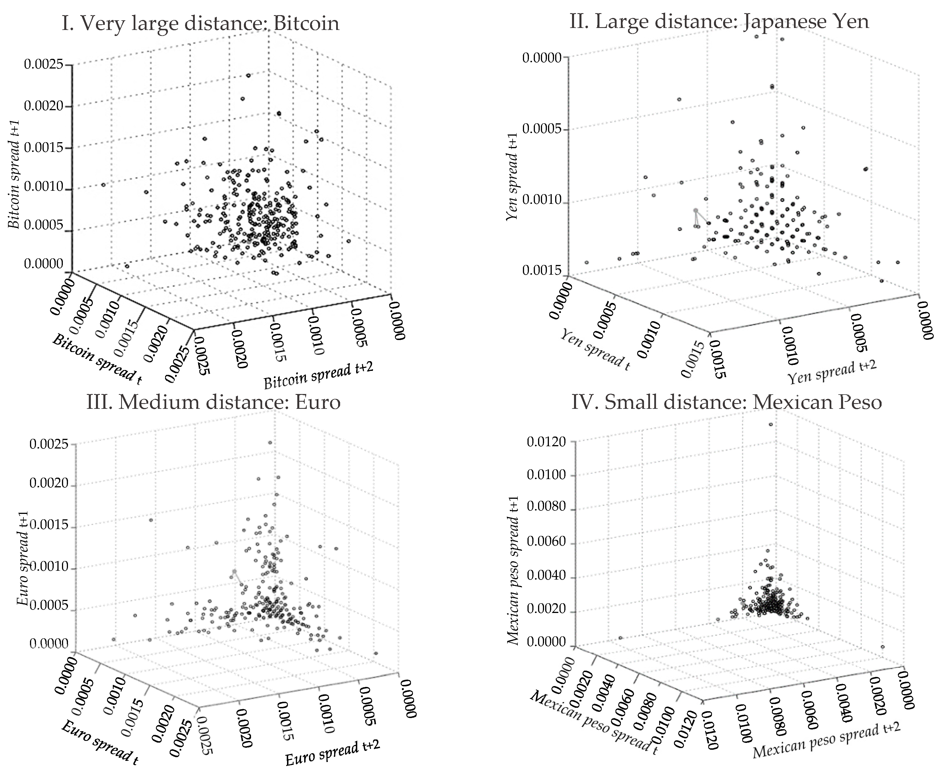
The last method applied to the log-rate series was the KNN approach. To choose the best number of k, we considered a range between one and five, with the lowest SSRs from the forecast. Figure 1 shows the predictor space charts based on three lags for the spreads of Bitcoin, euro, Japanese yen, and Mexican peso as examples to visualize the dispersion of the data. The points of the Bitcoin’s spreads are more dispersed over time than those visualized in fiat currencies, which are more concentrated between each other. For instance, the presence of outliers is more visible in the Mexican peso than the points in the space chart of Bitcoin. As it was noted in Table 2, the highest kurtosis was found in emerging countries’ currencies in comparison with cryptocurrencies. Therefore, due the complexity of the liquidity microstructure of cryptocurrencies, and hence the greater dispersions distance between each point of the chart space, more neighbor points should be considered to improve predictions compared with fiat currencies. Thus, based in the distance between each point and the neighbors, we classify the charts into four categories as follows:
- Very large distance: Bitcoin ( = 2), Ethereum ( = 3), and Ripple ( = 3)
- Large distance: Australian dollar ( = 2), Danish krone ( = 3), Japanese yen ( = 3), Norwegian krone ( = 2), and Taiwanese dollar ( = 2)
- Medium distance: British pound ( = 1), Canadian dollar ( = 2), euro ( = 2), Swedish krona ( = 3), and Swiss franc ( = 2)
- Small distance: Brazilian real ( = 2), Mexican peso ( = 1), New Zealand dollar ( = 1), Singaporean dollar ( = 1), South African rand ( = 2), and South Korean won ( = 1)
Figure 1 shows that the log rates of cryptocurrencies are more dispersed over time than are those of fiat currencies. For this reason, more neighbor points must be considered in cryptocurrencies than for fiat currencies to improve predictions. As an example of the KNN prediction, Table 5 shows the results for 6 February 2019, which is the third-to-last date of the study, as a selected focal case for the 19 currencies.
4.5. Comparative Analysis
Further, the SSRs for the three methods (ARMA, GARCH, and KNN) were calculated to compare the prediction ability and select the method with the minimum squared residual mean. Table 6 shows that the KNN approach produced the best results in predicting the spread of the log rates of the bid-ask spreads compared with the ARMA and GARCH models.
In terms of fiat currencies, the KNN approach provided the best prediction performance for the Canadian dollar, euro, and Japanese yen. In the case of cryptocurrencies, the prediction of the Bitcoin spread was better than that of Ripple and Ethereum.
5. Discussion
We compare the predictions on the short-term market liquidity of the major crypto and fiat currencies by using classical time-series models such as ARMA and GARCH and a nonparametric learning machine algorithm called the KNN approach. We find that the KNN algorithm is a better predictor of the log rate of the bid-ask spreads of crypto and fiat currencies than the ARMA and GARCH models given the nonlinearity of the market liquidity and the complexity of its market microstructure, as stated by Bouoiyour et al. [3].
We also find that the log rates of cryptocurrencies behave differently than those of the fiat currencies in developed markets. However, the short-term prediction (KNN approach) is similar in the emerging markets with fiat currencies when using a wider prediction timespan (GARCH model). The result of the cryptocurrency’s log rates is in accordance with its more complex pattern than the fiat currencies, as mentioned in Gandal and Halaburda [4], due to its time spatial dispersion performance derived from the KNN approach and with the absence of outliers, as noted by the kurtosis statistic.
Considering a classical time-series analysis, ARMA models are better at capturing the short-term liquidity of the fiat currencies in developed countries, whereas GARCH models are better suited for estimating the behavior of the fiat currencies in the emerging market countries because their currencies are more susceptible to sudden changes or unexpected news with a lower probability of following trends. Nevertheless, the KNN approach is better suited to capture the short-term liquidity of cryptocurrencies than the ARMA and GARCH models.
The practical implications of this study are twofold. First, as the number of entities that accept cryptocurrencies increases, this study shows that using the KNN approach better explains the short-term liquidity of the cryptocurrency market than traditional time-series models. This ability is important given the speculative nature of investors in the cryptocurrency market. Second, other machine learning models are worth trying to compare the results among them.
Despite the above results, three limitation of the study we can be observed. First, the sample used in this study is small because Bloomberg has a short time publishing cryptocurrencies data and it is difficult to obtain a reliable and complete data, i.e., bid-ask rates. Secondly, the cryptocurrencies analyzed in this paper is limited to three, and according to Ong et al. [52], there is a large array of cryptocurrency variants, alternative coins, or altcoins, that are introduced to the market on a daily basis; although, the information about cryptocurrencies can be sparse [53].
For future research, other type GARCH models could be reviewed in the comparison analyses, such as the VAR-BEKK-GARCH model proposed by Loverta and López [24] for log spreads times series. On the other hand, it is also possible to consider besides KNN other different intelligent algorithms that can be a route for cryptocurrencies behavior analysis, for example, the Support Vector Machine (SVM) and the Long Short-Term Memory (LSTM) model that was applied by Saadah and Wafa [36]. In addition, other possible direction for future research might include a systematic quantitative analysis of the popularity and impact of cryptocurrencies and how they spread in a macro level as suggested by Park and Park [54].
Finally, in this field it is necessary to deal with the interplay between liquidity, returns, and volatility in the context of long-term memory while at the same time using more nonparametric methods, such as machine learning, that may be better suited to deal with the microstructure complexity of the cryptocurrency markets.
Author Contributions
Conceptualization, K.C., M.d.P.R.-G. and S.M.; methodology, K.C.; software, K.C.; validation, K.C., M.d.P.R.-G. and S.M.; formal analysis, K.C., M.d.P.R.-G. and S.M.; investigation, K.C., M.d.P.R.-G. and S.M.; resources, K.C., M.d.P.R.-G. and S.M.; data curation, K.C.; writing—original draft preparation, K.C., M.d.P.R.-G. and S.M.; writing—review and editing, K.C., M.d.P.R.-G. and S.M.; visualization, K.C., M.d.P.R.-G. and S.M.; supervision, K.C. and M.d.P.R.-G.; project administration, K.C. and M.d.P.R.-G. All authors have read and agreed to the published version of the manuscript.
Funding
This article was written as part of a research project titled “Impact of technology on finance: evolution and future of Fintech” (PAICYT, CSA1312-20), which was sponsored by the Universidad Autonoma de Nuevo León.
Conflicts of Interest
The authors declare no conflict of interest.
References
- Balcilar, M.; Bouri, E.; Gupta, R.; Roubaud, D. Can volume predict Bitcoin returns and volatility? A quantiles-based approach. Econ. Model 2017, 64, 74–81. [Google Scholar] [CrossRef] [Green Version]
- Yermack, D. Is Bitcoin a Real Currency? An Economic Appraisal. In Handbook of Digital Currency: Bitcoin, Innovation, Financial Instruments, and Big Data; Chuen, D.L.K., Ed.; Academic Press: London, UK, 2015; pp. 31–43. [Google Scholar] [CrossRef]
- Bouoiyour, J.; Selmi, R.; Tiwari, A.K.; Olayeni, O.R. What drives Bitcoin price. Econ. Bull. 2016, 36, 843–850. [Google Scholar]
- Gandal, N.; Halaburda, H. Can we predict the winner in a market with network effects? Competition in cryptocurrency market. Games. SSRN Electron. J. 2016, 7, 16. [Google Scholar] [CrossRef] [Green Version]
- Dwyer, G.P. The economics of Bitcoin and similar private digital currencies. J. Financ. Stab. 2015, 17, 81–91. [Google Scholar] [CrossRef] [Green Version]
- Hayes, A.S. Cryptocurrency value formation: An empirical study leading to a cost of production model for valuing bitcoin. Telemat. Inform. 2017, 34, 1308–1321. [Google Scholar] [CrossRef]
- Nakamoto, S. Bitcoin: A Peer-to-Peer Electronic Cash System. Available online: https://bitcoin.org/bitcoin.pdf/ (accessed on 27 December 2016).
- Bas, D.S. Hayek and the cryptocurrency revolution. Iber. J. Hist. Econ. Thought 2020, 7, 15–28. [Google Scholar] [CrossRef]
- Encrybit Revealed Real-Time Cryptocurrency Exchange Problems—Survey Insights. Available online: https://medium.com/@enbofficial/encrybit-revealed-real-time-cyptocurrency-exchange-problems-survey-report-announced-650bba659a6d/ (accessed on 18 May 2020).
- Crook, M. Bringing liquidity to the new crypto economy. J. Digit. Bank. 2019, 3, 279–287. [Google Scholar]
- Jiang, S.; Li, X.; Wang, S. Exploring evolution trends in cryptocurrency study: From underlying technology to economic applications. Financ. Res. Lett. 2020, status (in press; corrected proof). [Google Scholar] [CrossRef]
- Dyhrberg, A.H.; Foley, S.; Svec, J. How investible is Bitcoin? Analyzing the liquidity and transaction costs of Bitcoin markets. Econ. Lett. 2018, 171, 140–143. [Google Scholar] [CrossRef]
- Wei, W.C. Liquidity and market efficiency in cryptocurrencies. Econ. Lett. 2018, 168, 21–24. [Google Scholar] [CrossRef]
- Sójka, B.B.; Hinc, T.; Kliber, A. Volatility and Liquidity in Cryptocurrency Markets—The Causality Approach. In Contemporary Trends and Challenges in Finance; Jajuga, K., Junge, H.L., Orlowski, L., Staehr, K., Eds.; Springer: Cham, Switzerland, 2020; pp. 1–43. [Google Scholar] [CrossRef]
- Brauneis, A.; Mestel, R.; Theissen, E. What Drives the Liquidity of Cryptocurrencies? A Long-Term Analysis. Financ. Res. Lett. 2020, status (in press; corrected proof). [Google Scholar] [CrossRef]
- Scharnowski, S. Understanding bitcoin liquidity. Financ. Res. Lett. 2020, status (in press; corrected proof). [Google Scholar] [CrossRef]
- Brauneis, A.; Mestel, R.; Riordan, R.; Theissen, E. How to measure the liquidity of cryptocurrencies? SSRN Electron. J. 2020, 3503507. [Google Scholar] [CrossRef]
- Hong, K. Bitcoin as an alternative investment vehicle. J. Inf. Technol. Manag. 2017, 18, 265–275. [Google Scholar] [CrossRef]
- Khuntia, S.; Pattanayak, J.K. Adaptive long memory in volatility of intra-day bitcoin returns and the impact of trading volume. Financ. Res. Lett. 2020, 32, 101077. [Google Scholar] [CrossRef]
- Phillip, A.; Chan, J.; Peiris, S. On long memory effects in the volatility measure of cryptocurrencies. Financ. Res. Lett. 2019, 28, 95–100. [Google Scholar] [CrossRef]
- Ruppert, D. GARCH Models. In Statistics and Data Analysis for Financial Engineering; Springer: New York, NY, USA, 2011. [Google Scholar]
- Nelson, D.B. Conditional heteroskedasticity in asset returns: A new approach. Econom. J. Econom. Soc. 1991, 59, 347–370. [Google Scholar] [CrossRef]
- Venter, P.J.; Maré, E. GARCH Generated Volatility Indices of Bitcoin and CRIX. J. Risk Financ. Manag. 2020, 13, 121. [Google Scholar] [CrossRef]
- Lovreta, L.; Pascual, J.L. Structural breaks in the interaction between bank and sovereign default risk. Ser. J. Span. Econ. Assoc. 2020, 11, 531–559. [Google Scholar] [CrossRef]
- Kyriazis, Ν.A.; Daskalou, K.; Arampatzis, M.; Prassa, P.; Papaioannou, E. Estimating the volatility of cryptocurrencies during bearish markets by employing GARCH models. Heliyon 2019, 5, e02239. [Google Scholar] [CrossRef]
- Walther, T.; Klein, T.; Bouri, E. Exogenous drivers of Bitcoin and Cryptocurrency volatility–A mixed data sampling approach to forecasting. J. Int. Financ. Mark. Inst. Money 2019, 63, 101133. [Google Scholar] [CrossRef]
- Acereda, B.; Leon, A.; Mora, J. Estimating the expected shortfall of cryptocurrencies: An evaluation based on backtesting. Financ. Res. Lett. 2020, 33, 101181. [Google Scholar] [CrossRef]
- Fakhfekh, M.; Jeribi, A. Volatility dynamics of crypto-currencies’ returns: Evidence from asymmetric and long memory GARCH models. Res. Int. Bus. Financ. 2020, 51, 101075. [Google Scholar] [CrossRef]
- Cerqueti, R.; Giacalone, M.; Mattera, R. Skewed non-Gaussian GARCH models for cryptocurrencies volatility modelling. Inf. Sci. 2020, 527, 1–26. [Google Scholar] [CrossRef]
- Köchling, G.; Schmidtke, P.; Posch, P.N. Volatility forecasting accuracy for Bitcoin. Econ. Lett. 2020, 191, 108836. [Google Scholar] [CrossRef]
- Stenfors, A. Bid-ask spread determination in the FX swap market: Competition, collusion or a convention? J. Int. Financ. Mark. Inst. Money 2018, 54, 78–97. [Google Scholar] [CrossRef] [Green Version]
- Kim, T. On the transaction cost of Bitcoin. Financ. Res. Lett. 2017, 23, 300–305. [Google Scholar] [CrossRef]
- Lahmiri, S.; Bekiros, S.; Salvi, A. Long-range memory, distributional variation and randomness of bitcoin volatility. Chaos Solitons Fractals 2018, 107, 43–48. [Google Scholar] [CrossRef]
- Khaldi, R.; El Afia, A.; Chiheb, R. Forecasting of BTC volatility: Comparative study between parametric and nonparametric models. Prog. Artif. Intell. 2019, 8, 511–523. [Google Scholar] [CrossRef]
- Saadah, S.; Whafa, A.A. Monitoring Financial Stability Based on Prediction of Cryptocurrencies Price Using Intelligent Algorithm. In Proceedings of the 2020 International Conference on Data Science and Its Applications (ICoDSA), Bandung, Indonesia, 5–6 August 2020; pp. 1–10. [Google Scholar]
- Devroye, L.; Gyorfi, L.; Krzyzak, A.; Lugosi, G. On the strong universal consistency of nearest neighbor regression function estimates. Ann. Stat. 1994, 22, 1371–1385. [Google Scholar] [CrossRef]
- Katsiampa, P. Volatility estimation for Bitcoin: A comparison of GARCH models. Econ. Lett. 2017, 158, 3–6. [Google Scholar] [CrossRef] [Green Version]
- Dickey, D.A.; Fuller, W.A. Distribution of the estimators for autoregressive time series with a unit root. J. Am. Stat. Assoc. 1979, 74, 427–431. [Google Scholar] [CrossRef]
- Box, G.; Jenkins, G. Time Series Analysis: Forecasting and Control, Time Series Analysis: Forecasting and Control; Holden-Day Inc.: San Francisco, CA, USA, 1976. [Google Scholar]
- Schwarz, G. Estimating the dimension of a model. Ann. Stat. 1978, 6, 461–464. [Google Scholar] [CrossRef]
- Akaike, H. A new look at the statistical model identification. IEEE Trans. Autom. Control. 1974, 19, 716–723. [Google Scholar] [CrossRef]
- Koehler, A.B.; Murphree, E.S. A comparison of the Akaike and Schwarz criteria for selecting model order. Appl. Stat. 1988, 37, 187–195. [Google Scholar] [CrossRef]
- Bollerslev, T. Generalized autoregressive conditional heteroskedasticity. J. Econ. 1986, 31, 307–327. [Google Scholar] [CrossRef] [Green Version]
- Mitchell, H.; McKenzie, M.D. GARCH model selection criteria. Quant. Financ. 2003, 3, 262–284. [Google Scholar] [CrossRef]
- Fix, E.; Hodges, J.L. Discriminatory Analysis, Nonparametric Discriminators: Consistency Properties; Technical Report 4; School of Aviation Medicine, Randolph Field: Texas, CA, USA, 1951. [Google Scholar]
- Cover, T.M.; Hart, P.E. Nearest neighbor pattern classification. IEEE Trans. Inf. Theory 1967, 13, 21–27. [Google Scholar] [CrossRef]
- Rubio, O.B.; Sosvilla-Rivero, S.; Rodríguez, F.F. Non-Linear Forecasting Methods: Some Applications to the Analysis of Financial Series; FEDEA Working Paper 2002-01; Fundación de Estudios de Economía Aplicada: Madrid, Spain, 2002. [Google Scholar] [CrossRef] [Green Version]
- Fernández-Rodríguez, F.; Sosvilla-Rivero, S.; Andrada-Félix, J. Exchange-rate forecasts with simultaneous nearest-neighbour methods: Evidence from the EMS. Int. J. Forecast. 1999, 15, 383–392. [Google Scholar] [CrossRef]
- Finkenstädt, B.; Kuhbier, P. Forecasting nonlinear economic time series: A simple test to accompany the nearest neighbor approach. Empir. Econ. 1995, 20, 243–263. [Google Scholar] [CrossRef]
- Arroyo, J.; Maté, C. Forecasting histogram time series with k-nearest neighbours methods. Int. J. Forecast. 2009, 25, 192–207. [Google Scholar] [CrossRef]
- Brock, W.A.; Scheinkman, J.A.; Dechert, W.D.; LeBaron, B. A test for independence based on the correlation dimension. Econ. Rev. 1996, 15, 197–235. [Google Scholar] [CrossRef]
- Ong, B.; Lee, T.M.; Li, G.; Chuen, D.L.K. Evaluating the Potential of Alternative Cryptocurrencies. In Handbook of Digital Currency: Bitcoin, Innovation, Financial Instruments, and Big Data; Chuen, D.L.K., Ed.; Academic Press: London, UK, 2015; pp. 81–135. [Google Scholar] [CrossRef]
- Jahani, E.; Krafft, P.M.; Suhara, Y.; Moro, E.; Pentland, A.S. Scamcoins, s*** posters, and the search for the next bitcoinTM: Collective sensemaking in cryptocurrency discussions. Proc. ACM Hum. Comput. Interact. 2018, 2, 1–28. [Google Scholar] [CrossRef]
- Park, S.; Park, H.W. Diffusion of cryptocurrencies: Web traffic and social network attributes as indicators of cryptocurrency performance. Qual. Quant. 2020, 54, 297–314. [Google Scholar] [CrossRef]
Figure 1.
Dispersion points in the predictor space chart for the k-nearest neighbor (KNN) approach. Source: Own elaboration with SPSS 21 from Bloomberg data.
Figure 1.
Dispersion points in the predictor space chart for the k-nearest neighbor (KNN) approach. Source: Own elaboration with SPSS 21 from Bloomberg data.


Table 1.
Depreciation rates, descriptive statistics.
| Currency | Mean a | SD a | Skewness a | Kurtosis a | ||||
|---|---|---|---|---|---|---|---|---|
| % | Rank b | % | Rank b | Value | Rank b | Value | Rank b | |
| Brazilian real | −0.049% | 15 | 0.973% | 05 | 0.697 | 02 | 3.242 | 01 |
| Ripple c | −0.342% | 18 | 6.355% | 01 | 0.737 | 01 | 2.170 | 02 |
| Ethereum c | −0.737% | 19 | 6.066% | 02 | 0.308 | 04 | 2.063 | 03 |
| Bitcoin c | −0.315% | 17 | 4.181% | 03 | −0.345 | 18 | 1.597 | 04 |
| Mexican peso | −0.004% | 02 | 0.785% | 06 | −0.398 | 19 | 1.478 | 05 |
| New Zealand dollar | −0.026% | 08 | 0.537% | 09 | 0.081 | 08 | 1.120 | 06 |
| Danish krone | −0.031% | 11 | 0.437% | 13 | −0.260 | 16 | 0.803 | 07 |
| British pound | −0.028% | 09 | 0.498% | 12 | 0.028 | 09 | 0.780 | 08 |
| Euro | −0.030% | 10 | 0.436% | 14 | −0.249 | 15 | 0.643 | 09 |
| Swedish krona | −0.051% | 16 | 0.585% | 07 | 0.223 | 05 | 0.602 | 10 |
| Japanese yen | −0.004% | 01 | 0.391% | 16 | 0.025 | 10 | 0.514 | 11 |
| Australian dollar | −0.036% | 13 | 0.553% | 08 | 0.003 | 11 | 0.435 | 12 |
| South Korean won | −0.009% | 04 | 0.501% | 11 | 0.092 | 07 | 0.389 | 13 |
| Taiwanese dollar | −0.018% | 05 | 0.270% | 18 | 0.187 | 06 | 0.384 | 14 |
| Swiss franc | −0.026% | 07 | 0.378% | 17 | −0.112 | 13 | 0.294 | 15 |
| Norwegian krone | −0.033% | 12 | 0.523% | 10 | −0.137 | 14 | 0.143 | 16 |
| Singaporean dollar | −0.008% | 03 | 0.265% | 19 | −0.020 | 12 | 0.099 | 17 |
| Canadian dollar | −0.020% | 06 | 0.426% | 15 | 0.341 | 03 | 0.067 | 18 |
| South African rand | −0.043% | 14 | 1.029% | 04 | −0.283 | 17 | −0.045 | 19 |
Notes: a Depreciation rates are calculated as the first logarithmic difference of the last prices. Prices are based on U.S. dollars. b Statistics are ordered from highest to lowest, and numbers in each rank’s column represent the place in the list of currencies. c Cryptocurrency. Source: Own elaboration with Eviews7 and data from Bloomberg.
Table 2.
Bid-ask spread rate (log-transformation), descriptive statistics.
| Currency | Mean | SD | Skewness | Kurtosis | ||||
|---|---|---|---|---|---|---|---|---|
| % | Rank a | % | Rank a | Value | Rank a | Value | Rank a | |
| Mexican peso | 0.097% | 10 | 0.090% | 10 | 6.895 | 03 | 74.027 | 01 |
| Singaporean dollar | 0.049% | 12 | 0.125% | 05 | 7.413 | 02 | 67.219 | 02 |
| South Korean won | 0.208% | 02 | 0.333% | 01 | 7.653 | 01 | 60.429 | 03 |
| South African rand | 0.299% | 01 | 0.232% | 02 | 3.635 | 04 | 17.463 | 04 |
| Brazilian real | 0.047% | 14 | 0.056% | 12 | 3.060 | 05 | 14.781 | 05 |
| New Zealand dollar | 0.192% | 03 | 0.177% | 03 | 2.836 | 06 | 13.686 | 06 |
| Swedish krona | 0.110% | 08 | 0.081% | 11 | 2.550 | 07 | 9.588 | 07 |
| Japanese yen | 0.024% | 19 | 0.023% | 19 | 2.356 | 10 | 7.302 | 08 |
| Canadian dollar | 0.045% | 15 | 0.045% | 15 | 2.548 | 08 | 7.232 | 09 |
| Swiss franc | 0.055% | 11 | 0.053% | 13 | 2.430 | 09 | 6.807 | 10 |
| British pound | 0.105% | 09 | 0.107% | 08 | 2.284 | 11 | 6.206 | 11 |
| Euro | 0.038% | 17 | 0.037% | 18 | 1.990 | 12 | 4.188 | 12 |
| Ethereum b | 0.134% | 06 | 0.108% | 07 | 1.870 | 13 | 4.099 | 13 |
| Norwegian krone | 0.169% | 05 | 0.120% | 06 | 1.732 | 14 | 3.860 | 14 |
| Australian dollar | 0.114% | 07 | 0.095% | 09 | 1.548 | 15 | 2.264 | 15 |
| Bitcoin b | 0.049% | 13 | 0.040% | 17 | 1.302 | 16 | 2.167 | 16 |
| Danish krone | 0.042% | 16 | 0.048% | 14 | 1.125 | 18 | 1.363 | 17 |
| Ripple b | 0.181% | 04 | 0.133% | 04 | 1.135 | 17 | 0.912 | 18 |
| Taiwanese dollar | 0.037% | 18 | 0.042% | 16 | 0.877 | 19 | −0.246 | 19 |
Notes: a Statistics are ordered from highest to lowest and numbers in each rank’s column represent the place in the list of currencies. b Cryptocurrency. Source: Own elaboration with Eviews7 and data from Bloomberg.
Table 3.
Augmented Dickey–Fuller test and ARMA(p,q) model.
| Currency | ADF a | ARMA(p,q) b | Dim2 c | Dim3 c | Dim4 c | Dim5 c |
|---|---|---|---|---|---|---|
| Canadian dollar f | −4.949 | 7,2 | 0.009 d | 0.009 d | 0.008 d | 0.006 d |
| British pound f | −2.940 | 5,8 | 0.003 d | 0.002 d | −0.002 d | −0.006 d |
| Ethereum | −3.725 | 5,7 | 0.014 | 0.020 | 0.026 | 0.030 |
| Australian dollar | −4.024 | 5,7 | 0.011 e | 0.019 | 0.023 | 0.020 e |
| Euro f | −4.023 | 5,5 | 0.007 d | 0.003 d | 0.004 d | −0.001 d |
| Japanese yen | −3.993 | 5,5 | 0.014 | 0.017 d | 0.019 d | 0.015 d |
| Danish krone | −4.881 | 5,5 | 0.012 | 0.018 | 0.026 | 0.027 |
| Mexican peso | −4.424 | 5,5 | 0.002 d | 0.014 d | 0.025 | 0.027 |
| South African rand f | −4.908 | 5,4 | 0.002 d | −0.001 d | −0.010 d | −0.016 d |
| Swedish krona | −5.232 | 5,4 | 0.034 | 0.044 | 0.039 | 0.036 |
| Norwegian krone | −4.298 | 5,4 | 0.018 | 0.032 | 0.036 | 0.036 |
| Swiss franc f | −4.260 | 5,0 | 0.014 e | 0.018 d | 0.017 d | 0.014 d |
| New Zealand dollar f | −4.910 | 4,5 | 0.009 d | 0.011 d | 0.008 d | 0.005 d |
| Bitcoin | −12.554 | 3,2 | 0.008 e | 0.018 | 0.022 | 0.025 |
| Taiwanese dollar f | −13.999 | 2,2 | 0.008 d | 0.009 d | 0.009 d | 0.010 d |
| Brazilian real | −8.028 | 1,2 | 0.007 d | 0.014 d | 0.021 e | 0.034 |
| Ripple | −2.913 | 1,1 | 0.016 | 0.033 | 0.039 | 0.042 |
| Singaporean dollar f | −16.508 | 1,0 | −0.015 d | −0.017 d | −0.017 d | −0.020 d |
| South Korean won | −16.017 | 0,1 | −0.014 d | −0.030 e | −0.041 | −0.034 e |
Notes: a ADF: Augmented Dickey–Fuller test statistic. b ARMA(p,q): Parameter p for the autoregressive model; table is ordered from highest to lowest p, followed by the parameter q for the moving average model. c Dim#: BDS statistic for dimension # from residuals. d H0:BDS = 0 is not rejected (5% significance, bootstrap probabilities). e H0:BDS = 0 is not rejected (1% significance, bootstrap probabilities). f There is no evidence to reject the hypothesis that the residuals of the model are iid (BDS test). Source: Own elaboration with Eviews7 and data from Bloomberg.
Table 4.
GARCH(1,1).
| Currency | ARCH a | GARCH b | Dim2 d | Dim3 d | Dim4 d | Dim5 d | ||
|---|---|---|---|---|---|---|---|---|
| Coeff. | Rank c | Coeff. | Rank c | |||||
| New Zealand dollar | −0.022 | 18 | 1.014 | 01 | −0.010 e | −0.023 f | −0.030 f | −0.033 |
| South Korean won g | 0.041 | 10 | 1.013 | 02 | 0.000 e | 0.000 e | −0.001 e | −0.001 e |
| British pound g | 0.031 | 13 | 0.939 | 03 | −0.002 e | −0.012 e | −0.026 f | −0.032 f |
| Swiss franc g | 0.037 | 11 | 0.936 | 04 | 0.000 e | −0.006 e | −0.013 e | −0.016 e |
| Canadian dollar | 0.023 | 14 | 0.907 | 05 | −0.006 e | −0.028 f | −0.049 | −0.056 |
| Euro | 0.016 | 15 | 0.886 | 06 | −0.005 e | −0.021 e | −0.032 f | −0.033 |
| Danish krone g | 0.016 | 16 | 0.862 | 07 | 0.008 e | 0.006 e | 0.003 e | 0.001 e |
| Japanese yen g | 0.050 | 09 | 0.839 | 08 | 0.002 e | 0.004 e | 0.002 e | 0.001 e |
| Bitcoin g | 0.111 | 07 | 0.835 | 09 | 0.000 e | −0.003 e | −0.003 e | −0.003 e |
| Taiwanese dollar g | 0.084 | 08 | 0.834 | 10 | 0.002 e | 0.009 e | 0.008 e | 0.005 e |
| Mexican peso g | 0.205 | 04 | 0.717 | 11 | −0.012 e | −0.022 f | −0.029 f | −0.032 f |
| Norwegian krone g | 0.036 | 12 | 0.712 | 12 | −0.003 e | −0.010 e | −0.010 e | 0.001 e |
| Ripple g | 0.262 | 03 | 0.663 | 13 | 0.002 e | 0.005 e | 0.000 e | 0.003 e |
| Brazilian real g | 0.491 | 01 | 0.644 | 14 | 0.004 e | 0.001 e | −0.004 e | 0.000 e |
| Ethereum g | 0.274 | 02 | 0.605 | 15 | 0.003 e | 0.003 e | 0.002 e | 0.001 e |
| Singaporean dollar g | −0.009 | 17 | 0.558 | 16 | −0.021 f | −0.027 e | −0.029 e | −0.032 e |
| Australian dollar g | −0.034 | 19 | 0.490 | 17 | −0.010 e | −0.017 e | −0.022 e | −0.022 e |
| South African rand g | 0.120 | 06 | −0.208 | 18 | 0.000 e | 0.004 e | −0.002 e | −0.010 e |
| Swedish krona g | 0.124 | 05 | −0.859 | 19 | 0.001 e | −0.002 e | −0.004 e | −0.002 e |
Notes: a Coefficient from GARCH(1,1) for square residuals lagged once. b Coefficient from GARCH(1,1) for conditional variance lagged once. c Coefficients are ranked from highest to lowest values. d Dim#: BDS statistic for dimension # from standardized residuals. e H0:BDS = 0 is not rejected (5% significance, bootstrap probabilities). f H0:BDS = 0 is not rejected (1% significance, bootstrap probabilities). g There is no evidence to reject the hypothesis that the standardized residuals are iid (BDS test). Source: Own elaboration with Eviews7 and data from Bloomberg.
Table 5.
Nearest neighbor predictions for 6 February 2019.
| Currency | Neighbor(s) a | Distance(s) b | Observed/Predicted c |
|---|---|---|---|
| 13 November 2018, 7 November 18, 21 November 2018 | 0.000002, 0.000003, 0.000005 | 0.000001/0.000001 | |
| Ethereum | 7 August 2018, 16 November 2018, 12 June 2018 | 0.000232, 0.000274, 0.000326 | 0.000727/0.000744 |
| Japanese yen | 26 December 2018, 14 February 2018, 27 September 2018 | 0.000112, 0.000141, 0.000194 | 0.000110/0.000111 |
| Ripple | 5 June 2018, 2 July 2018, 5 April 2018 | 0.000353, 0.000432, 0.000843 | 0.000000/0.000253 |
| Swedish krona | 25 April 2018, 26 September 2018, 24 October 2018 | 0.000174, 0.000254, 0.000259 | 0.000460/0.000470 |
| Australian dollar | 24 October 2018, 1 August 2018 | 0.000146, 0.000255 | 0.000281/0.000415 |
| Bitcoin | 16 April 2018, 11 September 2018 | 0.000094, 0.000084 | 0.000407/0.000404 |
| Brazilian real | 10 January 2019, 30 January 2019 | 0.000391, 0.00111 | 0.002959/0.002774 |
| Canadian dollar | 4 May 2018, 27 Abril 2018 | 0.000166, 0.00017 | 0.000529/0.000449 |
| Euro | 22 August 2018, 12 November 2018 | 0.000205, 0.000264 | 0.000176/0.000132 |
| Norwegian krone | 12 December 2018, 16 January 2019 | 0.000013, 0.00003 | 0.000854/0.000855 |
| South African rand | 9 May 2018, 17 October 2018 | 0.001357, 0.002655 | 0.002545/0.002034 |
| Swiss franc | 26 December 2018, 20 November 2018 | 0.000239, 0.000308 | 0.000301/0.000299 |
| Taiwanese dollar | 20 February 2018, 10 May 2018 | 0.00024, 0.000244 | 0.000555/0.000558 |
| British pound | 11 December 2018 | 0.000303 | 0.000696/0.000641 |
| Mexican peso | 14 November 2018 | 0.000295 | 0.000764/0.001021 |
| New Zealand dollar | 9 January 2019 | 0.00034 | 0.000885/0.000884 |
| Singaporean dollar | 21 February 2018 | 0.000786 | 0.000136/0.000265 |
| South Korean won | 21 January 2019 | 0.001488 | 0.000224/0.001702 |
Notes: a Nearest cases from the focal point (6 February 2019). b The distance between two cases (focal and its neighbor) is the sum, over all dimensions, of the absolute difference between values for the cases. c As a focal case, 6 February 2019, the third-to-last date of the study, was selected. Source: Own elaboration with SPSS21 and data from Bloomberg.
Table 6.
Sum-of-squares residuals (SSR).
| Currency | ARMA a | GARCH b | KNN c | |||
|---|---|---|---|---|---|---|
| SSR d | Rank e | SSR d | Rank e | SSR d | Rank e | |
| South African rand | 0.0010380 | 02 | 0.0037240 | 02 | 0.0000134 | 01 |
| New Zealand dollar | 0.0004680 | 03 | 0.0026110 | 03 | 0.0000078 | 02 |
| Mexican peso | 0.0001520 | 07 | 0.0004550 | 14 | 0.0000068 | 03 |
| Ethereum | 0.0000846 | 10 | 0.0007740 | 06 | 0.0000019 | 04 |
| Swedish krona | 0.0000825 | 11 | 0.0004860 | 12 | 0.0000017 | 05 |
| Ripple | 0.0002380 | 05 | 0.0022430 | 04 | 0.0000016 | 06 |
| Norwegian krone | 0.0001480 | 08 | 0.0020730 | 05 | 0.0000015 | 07 |
| Singaporean dollar | 0.0003930 | 04 | 0.0004710 | 13 | 0.0000014 | 08 |
| Australian dollar | 0.0000995 | 09 | 0.0005720 | 10 | 0.0000010 | 09 |
| British pound | 0.0001540 | 06 | 0.0005830 | 09 | 0.0000008 | 10 |
| South Korean won | 0.0028720 | 01 | 0.0039790 | 01 | 0.0000008 | 11 |
| Brazilian real | 0.0000651 | 12 | 0.0007250 | 07 | 0.0000004 | 12 |
| Swiss franc | 0.0000524 | 13 | 0.0001520 | 15 | 0.0000004 | 13 |
| Bitcoin | 0.0000283 | 16 | 0.0001020 | 17 | 0.0000002 | 14 |
| Danish krone | 0.0000307 | 15 | 0.0001060 | 16 | 0.0000002 | 15 |
| Taiwanese dollar | 0.0000373 | 14 | 0.0000810 | 18 | 0.0000002 | 16 |
| Canadian dollar | 0.0000275 | 17 | 0.0006370 | 08 | 0.0000001 | 17 |
| Euro | 0.0000136 | 18 | 0.0005300 | 11 | 0.0000001 | 18 |
| Japanese yen | 0.0000085 | 19 | 0.0000280 | 19 | 0.0000001 | 19 |
Notes: a Autoregressive moving average model. b Autoregressive conditional heteroscedasticity model. c Nearest neighbor approach. d SSR is the sum-of-squares residual from each model. e SSR are ordered from highest to lowest and numbers in each rank’s column represent the place in the list of currencies. Source: Own elaboration with SPSS21 and data from Bloomberg.
Publisher’s Note: MDPI stays neutral with regard to jurisdictional claims in published maps and institutional affiliations. |
© 2020 by the authors. Licensee MDPI, Basel, Switzerland. This article is an open access article distributed under the terms and conditions of the Creative Commons Attribution (CC BY) license (http://creativecommons.org/licenses/by/4.0/).
Share and Cite
MDPI and ACS Style
Cortez, K.; Rodríguez-García, M.d.P.; Mongrut, S. Exchange Market Liquidity Prediction with the K-Nearest Neighbor Approach: Crypto vs. Fiat Currencies. Mathematics 2021, 9, 56. https://doi.org/10.3390/math9010056
AMA Style
Cortez K, Rodríguez-García MdP, Mongrut S. Exchange Market Liquidity Prediction with the K-Nearest Neighbor Approach: Crypto vs. Fiat Currencies. Mathematics. 2021; 9(1):56. https://doi.org/10.3390/math9010056
Chicago/Turabian StyleCortez, Klender, Martha del Pilar Rodríguez-García, and Samuel Mongrut. 2021. "Exchange Market Liquidity Prediction with the K-Nearest Neighbor Approach: Crypto vs. Fiat Currencies" Mathematics 9, no. 1: 56. https://doi.org/10.3390/math9010056
Note that from the first issue of 2016, this journal uses article numbers instead of page numbers. See further details here.