Examining the Accuracy of GlobCurrent Upper Ocean Velocity Data Products on the Northwestern Atlantic Shelf


1
Ocean Process Analysis Lab, University of New Hampshire, Durham, NH 03824, USA
2
Department of Marine and Coastal Sciences, The State University of New Jersey, New Brunswick, NJ 08901, USA
*
Author to whom correspondence should be addressed.
Remote Sens. 2018, 10(8), 1205; https://doi.org/10.3390/rs10081205
Submission received: 29 June 2018
/
Revised: 26 July 2018
/
Accepted: 30 July 2018
/
Published: 1 August 2018
(This article belongs to the Special Issue Ocean Surface Currents: Progress in Remote Sensing and Validation)
Abstract
:This study provides a regional coastal ocean assessment of global upper ocean current data developed by the GlobCurrent (GC) project. These gridded data synthesize multiple satellite altimeter and wind model inputs to estimate both Geostrophic and Ekman-layer velocities. While the GC product was mostly devised and intended for open ocean studies, the present objective is to assess whether its data quality nearer the coast is suitable for other applications. The key ground truth sources are long-term mean and time series observations on the Northwestern Atlantic (NWA) shelf derived from Acoustic Doppler Current Profilers (ADCP) and high frequency (HF) radar networks in both the Mid-Atlantic Bight (MAB) and the Gulf of Maine (GoM). Results indicate that mean geostrophic currents across the MAB and the offshore GoM agree to roughly 10% in speed and 10 degree in direction with the in situ depth-averaged currents, with correlation levels of 0.5–0.8 at seasonal and longer time scales. Interior GoM comparisons at 5 coastal buoys show much less agreement. One likely source of GoM error is shown to be the GC mean dynamic topography near the coast. Comparison to near-surface MAB HF radar current measurements on the MAB shelf shows significant GC data improvement when including the surface Ekman term. Overall, the study results imply that application of GlobCurrent data may prove useful in coastal seas with broad continental shelves such as the MAB or Scotian shelf, but that large inaccuracies inside the GoM diminish its utility there.
1. Introduction
Satellite altimetry has become a key platform for routine ocean surface observations, making use of global sea surface height (SSH) estimates to resolve dynamic topography at the ocean mesoscale. Since the launch of TOPEX in 1992, numerous altimeter missions have followed including ERS, Jason, Envisat, AltiKa, CryoSat-2 and Sentinel 3A and 3B, and the likelihood of a sustained constellation into the future. It is now typical to have at least three polar-orbiting altimeters in operation at any time, yielding spatial coverage adequate for many mesoscale oceanography applications [1]. As a result, well-calibrated altimeter SSH data are increasingly available for deriving geostrophic ocean surface currents that permit improved observation and prediction of global upper ocean dynamics [2].
To first-order, absolute surface geostrophic current can be inferred by altimeter-based surface absolute dynamic topography (ADT), the sum of altimeter-measured sea surface height anomaly (SSHA) and an estimate of the mean dynamic topography (MDT). In the altimeter-centric approach, MDT is calculated as the mean sea surface (MSS) minus Geoid (G), that is, ADT = SSHA + MDT = SSHA + MSS − G. The accuracy of an altimeter-inferred absolute geostrophic current is then tied with those of SSHA as well as MDT that is related to both MSS and G. The quality of altimeter MSS estimates can be improved with longer-term altimeter SSH observations [3]. Recent MDT improvement has come from independent GOCE (Gravity and Ocean Circulation Experiment) mission data [3,4,5,6].
Geostrophic and wind-induced Ekman currents dominate ocean surface velocity variability on sub-tidal and longer time scales. While the altimeter community has been highly focused on geostrophic current, recent studies have also stressed the need to account for surface wind-induced Ekman contributions to the total surface current [7,8,9,10,11,12]. Thus, with the rapid growth in altimeter data now delivering broader coverage of geostrophic currents, it follows that available gridded global surface vector (2D) current products are now improving and that they also routinely include a wind-driven component based on Ekman theory to provide users with surface velocity estimates suited to numerous practical applications.
At present, the gridded surface vector current products are usually based on a combined geostrophic and Ekman current contributions, separately inferred from altimetry and weather model analysis winds, respectively. Optimal interpolation is used to statistically merge SSHA data from multiple altimeters onto a common grid and then to estimate geostrophic velocity, such as the gridded AVISO SSH and geostrophic current datasets [13]. These altimeter geostrophic velocity products are then augmented by adding wind-forced Ekman velocity contribution under ocean mixed layer model assumptions. Two such products are OSCAR (Ocean Surface Current Analysis (www.oscar.noaa.gov) [7,14] and GlobCurrent (www.globcurrent.org) [5]. For GlobCurrent, one point of emphasis has been the improvement of its underlying MDT estimates [5]. The latest GlobCurrent MDT product involved synthesizing global in situ observations (principally surface drifters and Argo floats) alongside prior direct estimates based on geoid and altimetry. In this way, MDT accuracy should improve upon that derived solely from the altimeter-based MSS and Geoid in regions where significant surface observations are available.
Although these global ocean current products are built primarily for open ocean applications without coastal optimizations, their gridded vector current format and continuous and multi-year content make them an attractive potential data source for shelf ocean and coastal applications. Recent dedicated coastal studies with satellite altimeter data suggest that further optimization and caution may be needed in using altimeter data close to the coast [15]. But several recent studies [16,17,18,19] on the Northwestern Atlantic (NWA) shelf region show great promise for application of standard altimeter-based along-track geostrophic current estimation approaches for shelf-slope process studies.
Previous validation studies of altimeter-based ocean currents have largely been focused on the analysis of along-track altimeter SSHA data where a single cross-track component of the current is derived, especially in coastal settings [8,10,11,12,16,17,20]. Such validations are usually limited to a few pre-existing in situ measurement locations that lie near a satellite ground track. Clearly, interpolation of these data away from each ground track may lead to errors, particularly where persistent geostrophic coastal or shelf break current locations are poorly-sampled by the available multi-mission altimeter (e.g., GlobCurrent) framework, and where bathymetric steering of currents induces anisotropy and inhomogeneity in the circulation that is poorly captured in the present optimal interpolation (smoothing) procedure. One distinction of the present study from these previous ones is the focus on gridded vector current products across the entire region using long-term and spatially extensive in situ datasets.
This study represents an attempt to ascertain whether global gridded multi-mission altimeter current velocity products are sufficiently accurate for coastal oceanographic applications on the NWA shelf. Specific study objectives are: (1) to evaluate GlobCurrent geostrophic currents against available in situ current measurement datasets obtained on two separate NWA shelf systems, the Gulf of Maine (GoM) and the Mid-Atlantic Bight (MAB), and (2) to quantify data product improvement gained by adding the wind-driven Ekman component.
2. Study Regions and General Oceanography
Figure 1 shows the chosen NWA study domain and two specific validation sub-regions. The GoM is a semi-closed marginal sea, set within the greater NWA shelf-slope system. By contrast, the MAB has a well defined wider continental shelf that extends south and southwest from Cape Cod. The MAB shelf topography is relatively smooth with depths increasing seawards from the coastline. The shelf width narrows southward progressively. Offshore, the adjoining NWA shelf slope sea has a generally SW mean flow extending from the Labrador Sea and Grand Banks, along the Scotian Shelf, and then on towards Cape Hatteras off the MAB shelf. The general along-shelf equatorward flow is modulated by various processes associated with shelf-slope, shelf-sea, and eddy-slope interactions occurring on a range of temporal and spatial scales. Processes including Gulf Stream induced eddies, strong topographic steering onshore of the shelf break from the Grand Banks through the Scotian Shelf, Georges Bank and on to the MAB, buoyancy runoff from regional rivers and higher latitude oceanic conditions, and extreme tides all contribute to shelf-sea circulation dynamics. These processes occur at a wide range of scales, not all of which are well resolved by satellite altimeter sampling. This presents both opportunities and challenges for the application of satellite-based ocean current data.
Specifics of the GoM circulation include persistent upstream transport from the Labrador Sea and the Gulf of St. Lawrence, as well as local fresh water runoff within the Gulf of Maine. The prevailing mean circulation pattern is counterclockwise around the Gulf. Its heterogeneous bathymetry leads to a self-contained system, largely isolated from the Atlantic and neighboring NWA shelf. Water mass exchange between the Gulf and NWA shelf occurs through several deeper channels—the Northeast and mid-Scotian shelf Channels (inflow) and the Great South Channel (outflow). These volume transports vary seasonally and inter-annually [17,18,21,22,23,24].
On the MAB, the along-shelf flow is sustained by alongshore wind stress, across-shelf buoyancy forcing due to an across-shelf salinity gradient, and an along-shelf pressure force associated with a large-scale surface slope [25,26]. Cross-shore momentum on the MAB shelf is nearly geostrophically balanced [27]. Lower salinity waters are separated from deeper slope waters by a sharp shelf-break front [28]. Eddy-shelf interactions associated with the Gulf Stream induced warm core rings also lead to cross shelf exchange with surface and sub-surface structure at scales of 10–30 km and days to weeks [29].
Over several decades the US Ocean Observing System has advanced to a point where monitoring of the GoM and MAB regions using in situ and satellite observations occur with sufficient frequency to begin to resolve variability at both seasonal and interannual time scales [16,17,18,19,22,30,31,32]. Thus, new scientific objectives are emerging tied to improved understanding of water mass mixing and transport variability associated with impacts of Scotian Shelf and Atlantic and Labrador Slope waters upon the GoM, Georges Bank, and MAB. Two recent studies [17,18] demonstrated that altimeter current measurements near the southwest Scotian Shelf provide new perspectives on the shelf transport variability, the former showing a high correlation with upper-ocean hydrographic changes downstream in the GoM. This finding suggests that long-term satellite altimeter observations (1992–present) offer valuable dynamic input for use in regional circulation models. Efforts in assimilative modeling using altimeter SSHA data on the GoM-MAB shelf are in progress [33,34]. Here we seek to apply these decade-long in situ ocean current datasets, recorded in both the MAB and GoM, to examine the accuracy of satellite-derived GlobCurrent data.
3. Data and Methods
The primary in situ ocean current datasets are from the US Integrated Ocean Observing System (US-IOOS). These include measurements from a GoM moored buoy network with Acoustic Doppler Current Profilers (ADCP) current time series from Northeast Regional Association of Coastal Ocean Observing Systems (NERACOOS, http://www.neracoos.org) and a MAB CODAR HF Radar network from the Mid-Atlantic Regional Coastal Ocean Observing System (MARACOOS) (see Figure 1).
3.1. Moored Buoy ADCP Observations in the GoM
In situ current measurements for the GoM portion of this study come from six met-ocean measurement buoys maintained by the University of Maine as part of NERACOOS. These buoys provide hourly measurements and are operated almost continuously, many from 2001 to present, with some limited data dropout periods and few data quality issues. Specific stations include those denoted as buoy L, I, E, and B that are moored along the coastline at 60–70 m depth, the latter three buoys within the nominally counterclockwise (CCW) inner Maine coastal current (MCC) (Figure 1). Buoys M and N are deployed in the deeper Jordan Basin and offshore Georges Basin/Northeast Channel, respectively. All buoys collect horizontal current measurements at 2–5 m vertical resolution from 10 m depth to near the bottom using ADCP. Buoy M and N measurements extend down to 200–300 m.
3.2. Depth-Averaged Mean Current Data in the MAB
An in situ current dataset obtained from Lentz [26] is available for GC current assessment. Lentz [26] compiled and developed an extensive observational annual depth-averaged mean current dataset to characterize the structure of mean depth-averaged vector current field on the MAB shelf. This dataset was based on various resources and generated in terms of historical MAB current-meter records longer than 200 days. The spatial coverage is relatively sparse and the measurement site distribution is not uniform, including sites on the southern flank of Georges Bank, on the New England shelf, and in the central and southern MAB (see Figure 1). Note that in this dataset (1) only depth-averaged mean vector currents are available and (2) bottom and measurement depths at individual sites are different. Details about the current-meter observations from each site can be found in Ref. [26].
3.3. CODAR HF Radar in the MAB
The second in situ current dataset in the MAB is from CODAR (Coastal ocean dynamics applications radar) HF (high frequency) radar that is a noninvasive system used to measure and map near-surface ocean vector current in coastal waters. In principle, HF radar uses the Doppler shift of a radio signal backscattered from ocean surface gravity waves to measure the-near surface current component in the radial direction of radar antenna [35,36]. By combining radial current components measured by two or more radar transmitters, maps of the surface vector current are obtained.
A MAB network of long-range CODAR HF radars has been in operation since at least 2004, and has provided the capability of monitoring surface vector currents from Cape Cod, MA to Cape Hatteras, NC over an along-shelf extent of approximately 500 km and a cross-shelf distance of about 90–130 km (Figure 1). This CODAR network is made up of a set of long range 5 MHz, standard range 25 MHz, and medium range 13 MHz sites (https://marine.rutgers.edu/marcoos/downloads/publications/MACOORA_HFGapFilling.pdf), directly supported by US-IOOS and MARACOOS.
The effective depth of the HF radar-derived surface current velocity is relatively shallow (of the order 1–3 m) and depends on different environmental factors, but mainly on the HF radar frequency. Stewart and Joy (1974) [37], showed that, for a linear surface current vertical profile, the effective measurement depth is proportional to the radar frequency. Ullman et al., 2006 [38] showed that the effective measurement depths are approximately ~0.5 m for the 25 MHz standard range system, and ~2.4 m for the 5 MHz long range system.
These MAB CODAR systems have supported numerous applications. For instance, a 25 MHz standard range system consisting of two shore stations with a coverage area of approximately 30 by 40 km and spatial resolution of 1.5 km has been used for inshore circulation studies [39,40,41]. For shelf-wide studies, a long-range 5 MHz system consisting of three shore stations covering an area of 250 km by 160 km is combined with 6 km resolution nearshore stations [42].
In this study, CODAR radial data are combined into hourly averaged total current vector maps on a fixed grid [39]. Since satellite GlobCurrent products contain no tidal terms, in our analysis the CODAR current time series at each grid point is de-tided by harmonic analysis of the principal tidal constituents [43]. The hourly de-tided CODAR currents are then interpolated onto a common grid with a spatial resolution of a 1/4° (~25 km) coinciding with the GlobCurrent product. The data used in this study cover a period from 2006 to 2017.
3.4. GlobCurrent Satellite Data Products
Satellite-based ocean current data for this study are the gridded Level 4 (L4) multi-mission GlobCurrent (Version 3.0) products. GlobCurrent data are chosen instead of OSCAR for this study in part because of GlobCurrent’s separate provision of Geostrophic and Total currents as well as the added efforts in developing a tailored data synthesis to improve the MDT [5]. We use the GC L4 gridded current products provided at a 1/4° spatial resolution, with the global Geostrophic-only current data at daily time step and the Total current data at a 3-hourly step. The Total vector current combines the Geostrophic and the Ekman component that is forced using 3-hourly wind stress from ECMWF ERA Interim datasets [45]. There are two available GlobCurrent products for the Ekman current components (and thus two products of Total currents). These are provided at two differing depths z. The first current product is at depth of significant wave height (i.e., at surface) and the second is at 15 m depth, referred to as 00 m and 15 m in results section, respectively. The GC Ekman currents are estimated using a 2-parameter empirical model by applying a least squares fit between estimates and simultaneous values of the ERA-Interim wind stress. In situ current datasets used for the empirical fitting of the Ekman model at their two product depths make respective use of surface drifter data and drifters drogued at 15 m depth. Description of this GC Ekman estimation approach can be found in Ref. [5]. In this study, these GC products cover the 23-year period from January 1993 to May 2016 and we use only the daily 00Z UTC datasets given that study interests are in sub-tidal and longer time scales.
3.5. Ocean Current Comparison Methods: GlobCurrent vs. In Situ
Daily GC vector component estimates are first spatially interpolated onto the locations of the selected in situ currents datasets. In situ current datasets are then averaged in time to match the daily GC resolution. This approach follows that of similar recent studies [7,8,10,16,17,46].
Effective evaluation of the GC currents at the two (surface and 15 m) depths requires consideration in the proper choice of in situ current measurement datasets. Previous studies [16,17] showed that depth-averaged upper ocean currents using ADCP profiler data yielded highest correlation with altimeter geostrophic current products in the offshore GoM. For the GoM data in this study, we will use depth-averaged (10–20 m) ADCP currents from each of the six GoM buoys to assess GC Geostrophic current and GC 15 m depth Total current (i.e., the sum of Geostrophic and 15 m Ekman currents). For the MAB data, there is access to two in situ datasets; the depth-averaged annual mean currents from Lentz [26] (Section 3.2) and the near-surface HF radar currents (Section 3.3). The choices made for MAB GC assessments are to compare GC Geostrophic and GC 15 m-Total current using the former, and to compare GC Geostrophic and GC Surface Total current at the depth of significant wave height using the latter.
Another specific GC validation issue requiring consideration is the choice of time and space scale for data evaluation. Recall that this dataset is a merged product combining multiple altimeter missions, each with exact repeat cycles no shorter than 10–35 days and with relatively wide inter-track spacing of 80–350 km. Thus, the effective spatial resolution of these L4 GC data depends on the number of altimeters in orbit at the particular time, as well as their collective orbit characteristics. In the best case, the average effective resolution of GlobCurrent is of the order of about 10 days and 100 km, though certain stations proximate to satellite ground track cross-overs the resolution may improve on this. Therefore, pushing validation of the GC Geostrophic component to time scales shorter than 10 days makes little sense. We choose to smooth both in situ and GlobCurrent time series data using a 70-day running mean low-passed (LP) filter to focus on seasonal and longer time scales. A running mean LP filter in this application sufficiently attenuates high frequency aliasing with a direct advantage of simplicity and near-equivalence to more advanced filtering approaches [17,30,46].
After filtering, linear regression analysis is performed between in situ and GlobCurrent current time series, including calculation of the effective number of observations and degree of freedom when estimating p-values and the 95% significance level in correlation analyses. Three qualitative statistical measures, Pearson correlation coefficient (R), root mean square error (RMSE) and bias (Bias) are used to assess altimeter GlobCurrent (A) current in terms of corresponding in situ measurement currents (M), as defined below,
where N is the sample number for matchup measurement pairs.
4. Results
For convenience, shorthand symbols are used hereafter to denote GlobCurrent (GC) products where the Geostrophic-only vector current is UG, and the total GC (Geostrophic and surface or 15 m Ekman) vector current is UGE00m or UGE15m. For in situ data, CODAR HF radar current are UHF and buoy measured depth-averaged current are UDA. The depth-averaged (10–20 m) current in the GoM buoys is further specified as UDA15m. For current components, eastward and northward components are denoted by lower-case letters u and v, and then as uG vG, uGE00m vGE00m, uGE15m vGE15m, and uDA15m vDA15m.
4.1. GC Comparisons with ADCP Observations in GoM: Mean Vector Currents
Long-term mean current vectors at the six GoM buoy locations are shown in Figure 2. This includes GC UG and UGE15m and buoy-measured depth-averaged UDA15m from depths of 10–20 m. The corresponding mean values are summarized in Table 1.
Results indicate that the accuracy of mean GC vector currents depends on the GoM location. In general, both UG and UGE15m shows best the agreement with UDA15m in both magnitude (within 20%) and direction at the most offshore buoy N location. This mooring is deployed in the eastern side of the northeast channel (NEC) near the offshore shelf break, and the mean velocity at buoy N is aligned with the NEC orientation, northwestward (~130° relative to the east, Table 1) into the GoM. Buoy-N UDA15m comparison with the GC Ekman-added UGE15m seen in Figure 2 improves upon the agreement seen with GC UG.
Discrepancies of GC data with buoys increase, however, inside the GoM. Visually, one observes only modest GC agreement between buoy-M UDA15m and UGE15m. The GC Ekman-added total UGE15m leads to a slightly improved agreement in both direction and magnitude with UDA15m. Turning attention to the GoM coastal buoy sites, GC estimates at buoys I, E or B lie far away from the observations. For example, GC estimates at Buoy I and E show opposing cross-shore flows that are both known to be unrealistic.
This overall disparity between mean GC and buoy vector currents in the interior GoM highlights one potential outstanding issue requiring consideration if GC coastal results are to improve. The issue is inherited from satellite altimetry, where repeated along-track measurements feed into the gridded mean sea surface (MSS) and geoid products and then into mean dynamic topography (MDT) grid used for GC product generation [4,5]. Error sources here include inaccuracies in short-scale geoid estimates and in data handling of the altimeter measurements impacted by altimeter geophysical correction limitations near the coast. To demonstrate, Figure 3 shows several different MDT estimates (GC uses MDTAVISO) along two separate satellite ground tracks (Jason and Envisat) in the GoM. Both repeating satellite passes (see Figure 2) transect Georges Bank and the western GoM. Results derived using solely the altimeter and geoid data (red and blue curves) show unphysical short wavelengths that likely arise from errors in the geoid model [47]. These may be expected from gravity anomalies in shallow, coastal seas on continental margins with complex bathymetry. Also shown is the MDT based on statistical and dynamical analyses of ocean circulation; namely, the MDTAVISO by Rio et al. [4] (light blue line). The final product shown in Figure 3, MDTRU (black curve), is a result obtained from a hydrodynamic circulation model constrained by variational data assimilation of a regional hydrographic climatology of temperature and salinity, and long-term mean velocity from HF-radar, shipboard ADCP, current-meters and surface drifters following the same approach described by Levin et al. [48].
What is most salient for improved coastal current estimation is that MDTRU correctly captures an expected upward MDT slope approaching the coast north of 43N (i.e., the mean coastal setup). This is associated with the narrow equatorward Maine Coastal Current in the GoM. This slope is actually reversed in MDTAVISO, which would bias the directionality of absolute geostrophic flow based on MDT plus altimeter SSHA. On other GoM altimeter ground tracks (not shown), strongly contradictory and erroneous MDTAVISO results are also observed along this MCC region. In all, this analysis suggests that MSS and geoid errors require further attention and likely factor into the poor interior GoM performance of the mean GlobCurrent estimates.
4.2. GC Comparisons with ADCP Observations in the GoM: Temporal Variability
Long-term in situ buoy measurements permit straightforward assessment for GC’s ability to reproduce temporal variability observed at each buoy location in the GoM. Statistical measures for UG and UGE15m vs. buoy depth-averaged (10–20 m) UDA15m are calculated for the eastward (u) and northward (v) components, using 70-day running mean LP time series. Results are summarized in Table 2 and Figure 4 and Figure 5.
Figure 4 shows more than a decade of current time series at two of the six buoy sites, N, and I. These time series are shown as examples of locations displaying both high (buoy N) and low agreement (buoy I) with the in situ data. Both u and v component data are shown.
It is evident in Figure 4a that both GC UG and GC UGE15m are similar and are highly correlated with buoy-N data for much of the time records and for both u and v components. Quantitatively, Table 2 indicates higher correlation is seen for u than for v. There is also a slight increase in R values for Ekman-added GC as compared to the Geostrophic for both u and v (Figure 4a) with correlation values of ~0.77–0.78 for uG and uGE15m, and 0.46–0.53 for vG and vGE15m. The bias between GC and buoy data is within [−0.4, 0.6] cm/s. RMSE between GC uG (and uGE15m) and in situ uDA15m are approximately 3.4 cm/s. This is lower than the standard deviation (5.4 cm/s) of in situ buoy-N uDA15m (see Table 2). RMSE between GC vG and vGE15m, and buoy vDA15m are 4.4 and 4.2 cm/s, similar to the standard deviation level (4.3 cm/s) of buoy N vDA15m.
Inside the GoM, generally consistent with mean vector current comparisons shown in Figure 2, GC data quality again degrades significantly. Comparison details depend on the buoy site and vector components as well (Table 2). As one example, buoy-I results (Figure 4b) indicate that despite a high bias (~8–9 cm/s for the eastward component), time-variable content in the GC data show some agreement with buoy-I ADCP observations. In particular, the eastward component UG and UGE15m data show R values of 0.37 and 0.30 with UDA15m and generally similar peak-to-peak variation with season. However, this is not the case for the northward component VG, nor VGE (the lower panel in Figure 4b). This is certainly in part due to the fact that alongshelf current at buoy I is oriented mostly in the E-W and is much stronger than the cross-shore current at this site (see UDA15m vs. VDA15m in Figure 4b). But one also observes that the rms variation (i.e., standard deviation) of northward GC data in Figure 4b is much larger than the actual ADCP data by a factor of two (see Table 2). This increase appears to be erroneous signal due primarily to the geostrophic component in the GlobCurrent product.
The high comparison bias seen again for both GC UGE15m and UG is most likely tied to an inaccurate MDT, particularly in the GoM shelf close to the coast, as illustrated in Figure 3. The RMSE between GC UGE15m and UDA15m at buoy I site is 4.6 cm/s, about the same magnitude as the standard deviations of buoy-I uDA15m, 4.4 cm/s (see Table 2). Time series for the other buoys are not shown here, but GC data performance at these mostly coastal locations does not improve measurably beyond that seen at Buoy I.
To summarize the overall location-specific GoM GC product performance, Figure 5 graphically presents these statistical measures corresponding to the GC current u- and v-component against the in situ data. Details drawn from Figure 5 and Table 2 include:
- For most statistical measures, eastward GC components (either uG or uGE15m) perform much better than northward components, vG and vGE15m.
- GC data agreement is worst at buoy L. This may stem from buoy L having the shortest measurement time period (less than 5 years) or from site-specific circulation dynamics.
- At buoy M there is significant, but marginal correlation (~0.42–0.45) for uG and uGE15m, and clearly the Ekman addition enhances GC accuracy.
- For the GoM nearshore sites, relatively better performance for the eastward component is seen in the east (buoy I) than in the west coast (buoys E and B), with correlations and RMSEs measurably degrading from the east to the west. This may be tied to the distinct hydrographic properties between the eastern and western coastal shelf as well as GC MDT errors.
- Finally, the addition of a wind-driven Ekman component to the total does not lead to measurable GC product improvement in the GoM coastal sites.
4.3. GC Comparisons with Lentz’s Data in the MAB: Mean Vector Currents
In lieu of long-term buoy data available in the GoM, GC mean flow characteristics are assessed in the MAB by using the depth-averaged mean current UDA dataset from Lentz [26]. Here we just term the current in this dataset UDA [26] because measurement depths at individual sites are different. GC comparison results at representative study locations are given in Table 1 and a subset of those are shown in Figure 6.
GC UG and UGE15m estimates at most MAB locations show generally good agreement with the depth-averaged mean vector current UDA [26] (Figure 6), particularly nearer to the shelf break. Consistent with the well-documented mean circulation characteristics on the MAB shelf, both the GC UG and UGE15m mean flow estimates follow the in situ data in showing an equatorward and approximately along-shelf direction. An exception to this, as mentioned by Lentz [26], is the flow within the Hudson shelf valley off Long Island (near 40.0N, 73.5W) and the largest GC estimate discrepancies are found near this sub-region.
Overall, GC UGE15m data in Figure 6 show that the Ekman-added total UGE15m leads to GC flow that is 0°–10° and 10°–30° CCW from GC UG and UDA (also see Table 1), respectively. This indicates an increase in the offshore flow component and is consistent with the impact of a mean local SE wind stress [26]. In fact, these CCW changes generally increase the discrepancy between the GC UGE15m and in situ UDA data across the measurement locations. In general, a slightly better overall agreement with UDA is obtained versus UG (Geostrophic) rather than the GC Ekman-added total UGE15m estimate. This finding is not unexpected because the depth-averaged mean currents are likely dominated by geostrophic rather than surface Ekman-layer control. Furthermore, we do see the site dependent discrepancies between GC UG and in situ UDA, as well as GC UGE15m and in situ UDA. Specifically, the in situ depth-averaged mean UDA currents appear smaller in magnitude than GC products in most of the sites. These discrepancies may be attributed to the fact that the in situ UDA from [26] is the one averaged over a depth mostly deeper than 15 m—the Ekman depth provided in the GC Ekman current component. As a result, the in situ depth-averaged UDA currents appear slightly below the GC products in these sites. In addition, these discrepancies may also be related to other factors such as stratification-induced baroclinicity and ageostrophic components.
In the next section, HF radar observations of near-surface currents are used to further examine the impact of the Ekman component.
4.4. GC Comparisons with HF Radar Data in the MAB: Mean Vector Currents
The fine spatial coverage obtained with HF radar observations offers the opportunity to assess both the spatial content and Ekman-related content in the gridded GC products. As mentioned before, the efficient HF radar measurement depth lies between 0.5–2.4 m. Thus, UHF data are best used to assess GC UGE00m (Geostrophic + Surface Ekman). For completeness, we also assess GC UG vs. UHF to quantify the impact of the Ekman-added currents on GC data performance.
Here, we examine the mean currents and the differences between GC UGE00m (and UG) and UHF across the MAB (Figure 7). At the outset, there are evident distinctions between the in situ UHF data and the UDA by Lentz [26] shown in Figure 6. A stronger offshore flow component clearly exists in UHF, particularly on the northern part of the MAB shelf (above 39.5N, 72W). On the southern shelf, UHF and UDA are more generally consistent.
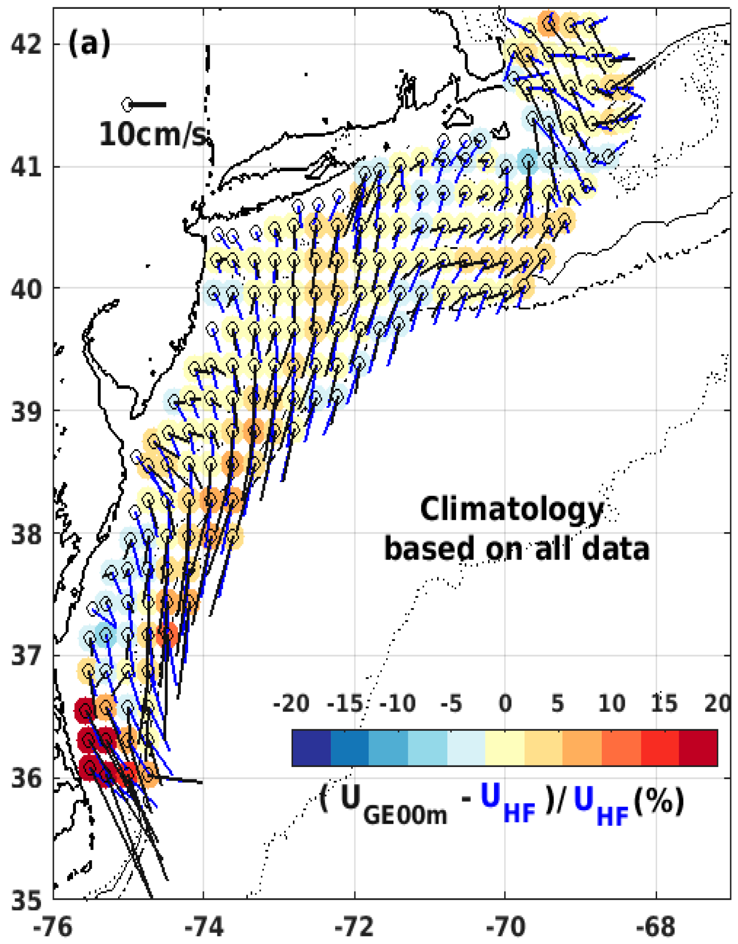
Figure 7a,b respectively display the spatial content of the comparison between the mean GC UGE00m and UG vectors alongside UHF data averaged from 2006–2016. In general, the magnitude percentage differences are well within ±10% for both cases, UGE00m vs. UHF and UG vs. UHF. When considering both direction and speed, it becomes clear that GC UGE00m shows an improved performance across most of the shelf. The improvement in current direction estimates due to the addition of surface Ekman currents is especially obvious along the shelf break front. However, whereas UGE15m direction fell CCW from in situ UDA in the comparisons shown in Figure 6, it now falls CW from UHF, especially in the northern MAB.
The percentage differences in current magnitude between GC UGE00m (or GC UG) and UHF are well within the range of ±10% (this can translate to absolute differences of about ±4 cm/s) on most of the shelf. In the northern shelf, the magnitude percentage differences between UGE00m and UHF are slightly smaller than those between UG and UHF. This is not true however for the narrower southern-most shelf or steeper shelf break front regions where the magnitude differences between both GC UGE00m and GC UG vs. UHF increase to larger than +10% (GC overestimate), largest for GC UGE00m vs. UHF. The highest mean current magnitude % difference up to +20% (about +8 cm/s in absolute) occurs south of the Chesapeake Bay. It is unclear if the source of this difference lies in the altimeter or in situ data.
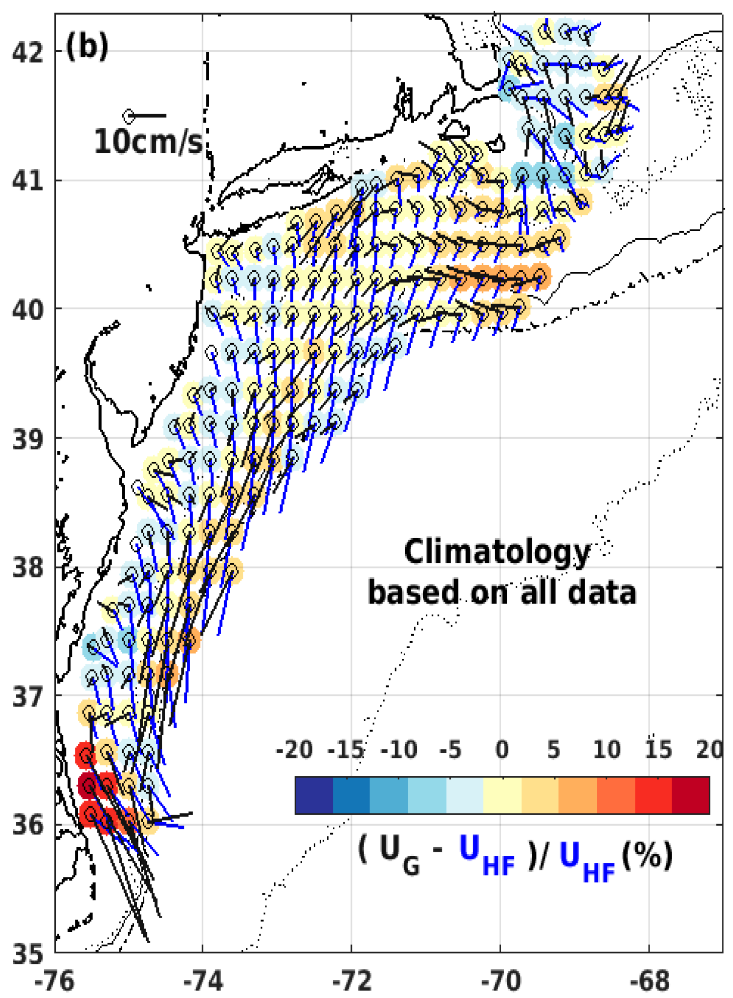
To more fully assess the wind-driven impact on the GC product, similar spatial mappings were broken out by season. The most insight is likely found for the winter when the wind stress is highest. In winter, as seen in Figure 8, it is apparent that: (1) for the mid and northern shelf, the % difference in magnitude between UGE00m and UHF is generally smaller than or similar to those between UG and UHF; (2) the % differences between UGE00m and UHF, and UG and UHF are over- and under- estimated, respectively, apparently towards the narrower southern shelf, and (3) the largest improvement due to the Ekman added total current is that the mean current directions of GC UGE match those of UHF much better than GC UG on the entire MAB shelf. Comparisons in the other seasons (not shown) exhibit qualitatively similar changes but with lower impacts.
4.5. Comparisons with HF Radar Data in the MAB: Temporal Variability
To examine how well GC UGE00m and UG reproduce seasonal temporal variability observed by the MAB HF radar data, as shown in Figure 1, five focus areas are selected for evaluation. Areas A and B represent shelf sites with less than 100 m water depth on the wider northern MAB shelf where the flow is oriented more in the E-W direction. Areas C-E fall along shelf break front over the 90–450 m isobaths, from the north to the south, respectively. As above for the GoM, statistical measures are calculated to assess the accuracy of GC currents. Results are presented in Figure 9 and Figure 10 and Table 3.
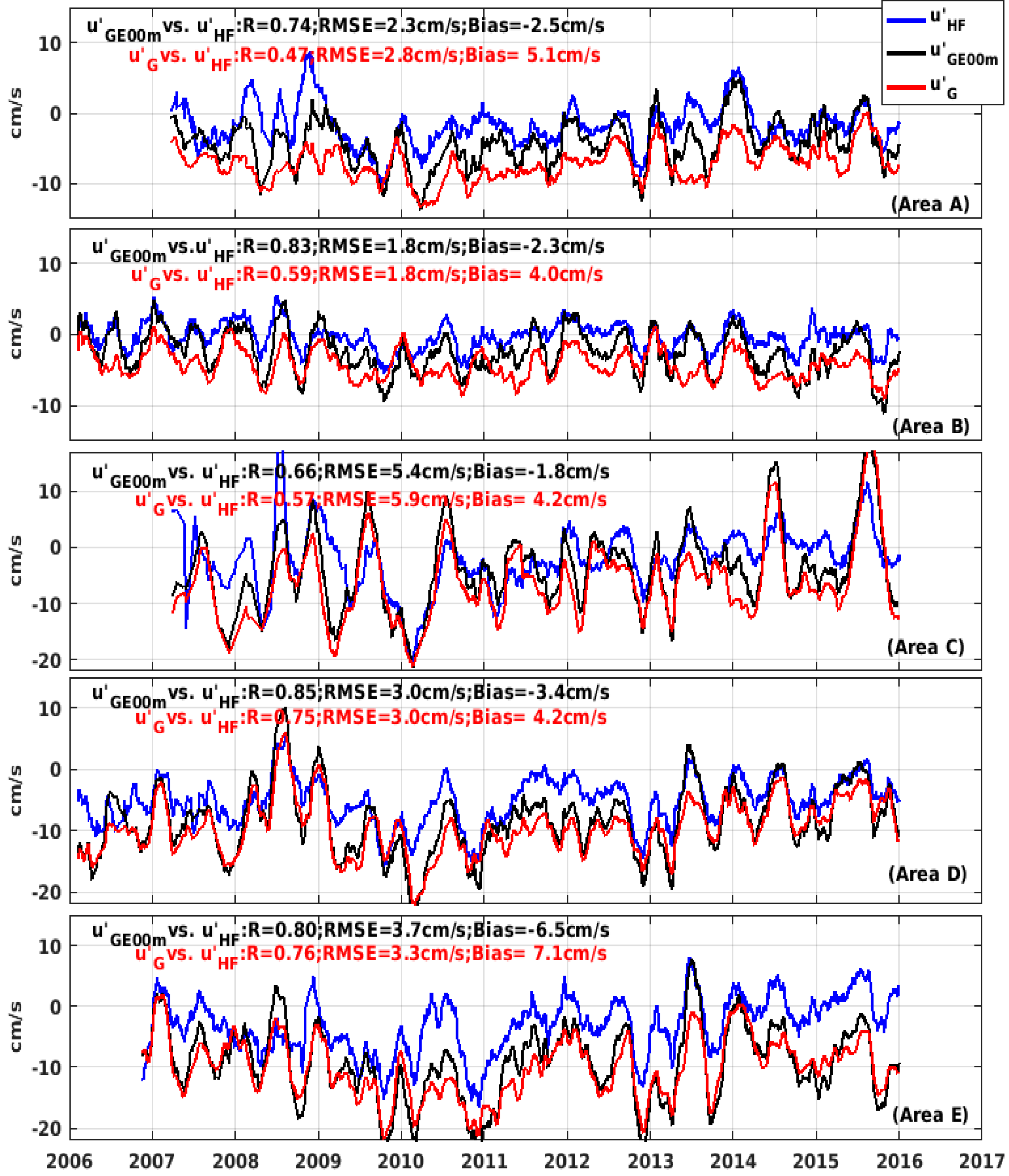
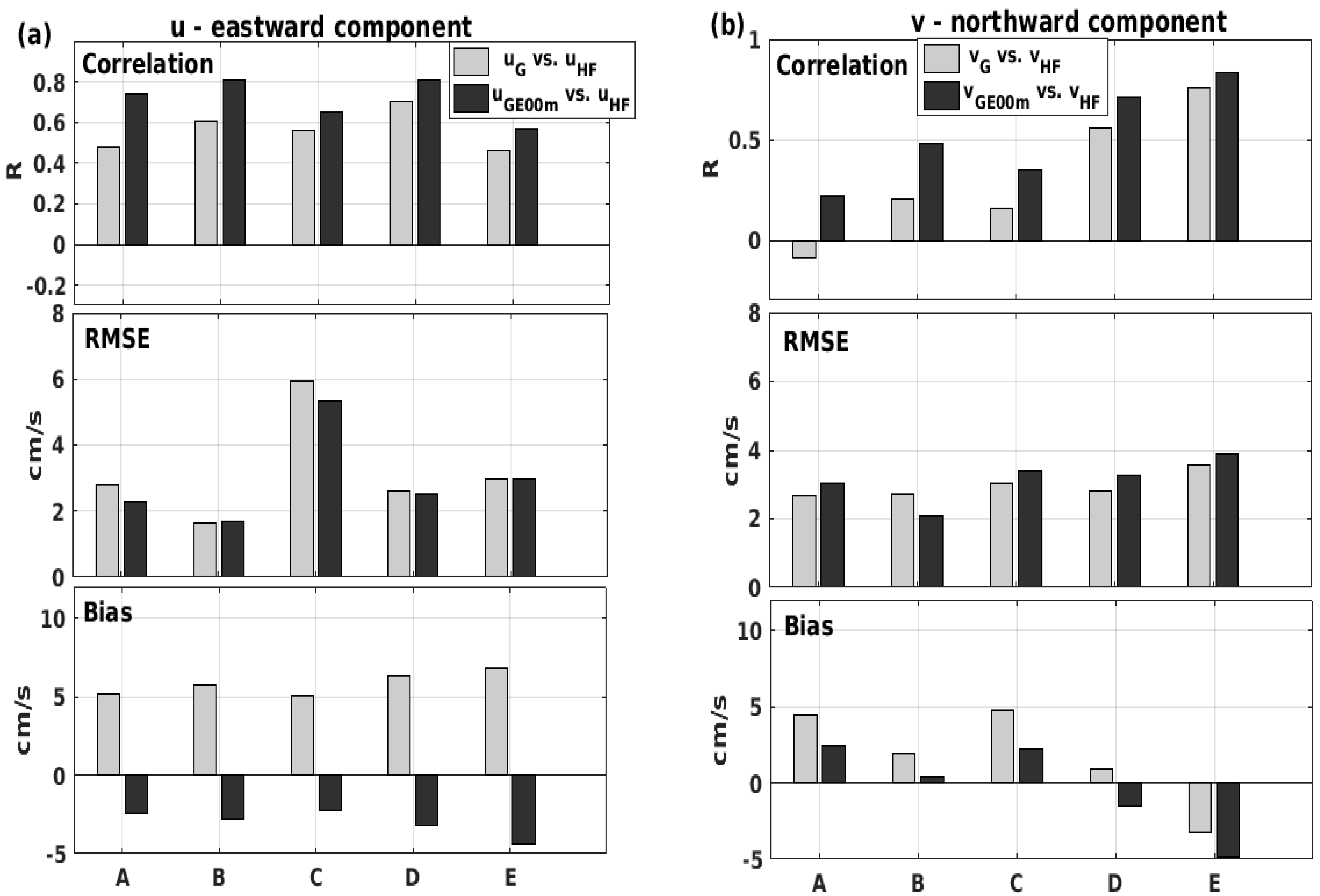
As well known, the dominant flow in the MAB shelf is alongshelf and mainly equatorward. Thus, GC and HF radar components are projected onto the local isobath-aligned alongshelf and cross-shelf components denoted in [u’, v’]. The collocated 9-year time series of the alongshelf component u’ are presented in Figure 9 for all five selected areas. The HF radar and two GC estimates all exhibit significant seasonal and interannual variability with more enhanced interannual variation seen along the shelf break areas C–E. Amongst the three records, moderate coherence is seen across all five areas, but the level of agreement varies. For this alongshelf current component, the statistical comparison results provided in Figure 9 clearly reveal measurably better agreement of GC u’GE00m with u’HF than GC u’G. Correlation coefficients improve by 10–30% across all five areas, improving from R = 0.44–0.76 for geostrophic-only GC u’G data to R = 0.66–0.85 for GC surface total u’GE00m. The correlation for the alongshelf current u’ appears the lowest (0.57–0.66) in the upper MAB shelf break (area C) and becomes higher in the lower MAB shelf break (areas D and E). A close inspection of seasonal alongshelf current variations in Figure 9 shows the occasional strong discrepancies between GC u’GE00m and u’G data where the former shows much stronger seasonal variability and better temporal agreement with the HF radar u’HF.
Figure 10 graphically presents these performance measures for the GC eastward u- and northward v- component against in situ HF ones. Calculated measures are given in Table 3.
Another notable change is the global shift in the sign of the bias for uGE00m (Figure 10a), consistent with the mean directional shift seen in Figure 7a vs. Figure 7b due to the mean winds. This is confirmed by the Table 3 results that show, for all five areas, an increased standard deviation in uGE00m vs. uG, but almost uniform improvement in the comparison RMSE with uHF when adding the Ekman-driven currents.
Performance results for northward component data are seen in Figure 10b and Table 3, excepting markedly lower correlation for areas A–C where the mean current is oriented more in the E–W. Figure 10b shows that the VGE00m vs. VG comparisons change across areas A-E, both in terms of correlation (improve for A–E) and bias (mostly decreased for A–E). The order of these A–E areas roughly follows the E–W to N–S turn of the alongshore MAB current as seen in Figure 6. As for the eastward component, the northward Ekman-added GlobCurrent VGE00m performs better than VG.
5. Discussion and Conclusions
Study results show uneven GlobCurrent data performance between our two sub regions, with generally better comparisons in the Mid Atlantic Bight. This is not wholly unexpected for several reasons. Foremost, the prevailing ocean circulation on the wider shallow MAB is more homogeneous and dominated by balance between geostrophic, bottom friction, and wind stress controls [26]. By contrast, the highly variable bathymetry of the Georges Bank and Gulf of Maine system leads to much greater spatial variation in the mean current field and geostrophic vs. ageostrophic controls. Sub region data assessment contrasts also result from the differing available in situ datasets, shelf-wide HF radar and depth-averaged current study sites by Lentz [26] in the MAB versus six long-term ADCP moorings in the GoM. The detailed data comparisons in Table 1, Table 2 and Table 3 generally document regional GlobCurrent data accuracy, but these MAB and GoM study contrasts are large enough that data discussion is separated to highlight key findings that can be drawn given these distinctions.
Starting with the MAB and the central GlobCurrent product, the geostrophic current (UG), Table 1 indicates that there is remarkably close directional agreement between the depth-averaged mean current at 15 of the 19 shelf locations of the data gathered by Lentz [26]. The average difference is +5.8 deg, slightly seaward of the in situ observations. GlobCurrent magnitudes show a slight positive bias in general but are also in close agreement (<15%) for most of the MAB. The exception is the southern-most region near Cape Hatteras and the Gulf Stream (36.24S, Table 1) where overestimations of 100–400% are seen. Data discrepancies for this narrow shelf area in the south were also found in the HF radar comparisons (Figure 7 and Figure 8) and are left for future examination. Most of the MAB focus here is north of 38N.
Turning to the HF radar comparisons to mean GlobCurrent UG fields in the MAB (Figure 7b), it becomes apparent that the altimeter-derived geostrophic currents show a persistent onshore directional bias with respect to HF radar current direction. This bias is certainly attributed to the CCW directional change between the GC UG and UHF driven by prevailing SW wind stress. It is also consistent with previous coastal sea findings that altimeter-derived GC UG shows high correlation with surface layer currents averaged vertically down to 40–50 m [17,46].
Given the nearer-surface content of the MAB HF radar currents, one expects better comparison with the GlobCurrent UGE00m data, rather than UG. This is borne out in Figure 7, Figure 8, Figure 9 and Figure 10 and Table 3. UGE00m shows clear improvement in directional agreement when comparing Figure 7a vs. Figure 7b. An improvement to the negative GlobCurrent UG bias in mid-shelf MAB data is also observed when comparing the percentage difference information. The directional impact of adding the surface Ekman component into the GlobCurrent estimates is most visible in the winter period, as illustrated in Figure 8. It is because the wind stress is highest in the winter time. Quantitatively, Figure 10 and Table 3 show that there are almost uniformly positive impacts on the correlation coefficients (10–50%) and on bias reduction (50–100%) when using UGE00m vs. UG.
The ability of GlobCurrent data to capture time variable MAB content at seasonal and longer scales is assessed only using HF radar observations. Correlation coefficients on vector components can be as high as 0.83 (Table 3). The MAB alongshelf current component time series in Figure 9 show frequently close agreement with large-scale interannual variation (e.g., 2009–2012 for Area C). Yet these data are also provided to show users the magnitude of the remaining discrepancies (unresolved variance is often greater than 50%), as well as the extent of increases in seasonal variation gained for UGE00m vs. UG data in the MAB. As noted earlier, results in Figure 9 and Figure 10 also reflect the turn in alongshore flow direction from areas A to E that shifts the dominant current from zonal to meridional direction.
Turning to the GoM results, one strength of the datasets is the ability to obtain sub-daily UDA15m observations over 10–15 year time periods for comparison with GlobCurrent data. A limitation is that these 4 out of 6 moorings are located within 10–20 km of the coast where altimeter measurements become questionable [16,17]. The GoM GlobCurrent assessments should bear this out. The best performance, by far, is found at the most offshore Buoy N site as seen in Figure 2 and Figure 5. GC mean vector currents UGE15m and UG agree very well with UDA15m, particularly for UGE15m vs. UDA15m (Figure 2 and Table 1). Observed correlations are 0.78 and 0.53, RMSEs are 3.4 and 4.2 cm/s for the GC eastward UGE15m and northward VGE15m currents (Table 2), respectively. The RMSE levels are slightly lower than the standard deviations (5.4 and 4.3 cm/s) of buoy-N UDA15m and VDA15m. In the previous validation study [17], the cross-track (i.e., across the Northeast Channel) geostrophic current anomaly was estimated using single-track TOPEX and Jason satellite data near buoy N to find R = 0.64 and RMSE 3.3 cm/s. This present new GC evaluation suggests the GC product has at least maintained or enhanced the quality compared to altimeter current datasets from along-track SSHA analysis. Time series data of Figure 4a show that GlobCurrent UG carries much of the temporal variability at this buoy-N site in reasonably close agreement with the UDA15m data. We do however see a modest improvement in correlation, but a positive impact on bias when comparing UGE15m in place of UG. A fine point tied to the time-variable quality of multi-mission GlobCurrent data may be seen in the northward component data in the lower panel of Figure 4a. It is known that there was an interleaved Jason-1 and Jason-2 satellite orbit period (January 2009–June 2013) when satellite altimeter ground track coverage improved to provide added sampling of the northward current across buoy N. Improved correlation with UDA15m is apparent. With such longer time series datasets, it may thus be feasible to document such space/time GlobCurrent data uncertainties.
Inshore of buoys, GlobCurrent UG or UGE15m data agreement with both the mean and the time-variable content in UDA observations is poor at all other buoy sites (Figure 2, Figure 4b and Figure 5). This is especially true for the mean current vector along the northern coastal buoys (I, E, B) that lie in a known along-shore coastal current [49]. There is perhaps some potential for resolving this alongshore current eventually as there is a weak, but statistically significant correlation in UGE15m of R = 0.17–0.31 (Table 2). To this point, a likely cause for this discrepancy in the mean is identified in Figure 3 where an inaccurate local MDT product is presently used by GC to derive absolute currents along this GoM coastline region. Time series analysis at the more offshore Buoy M was not shown in the study but, just as for 2009–2013 Buoy N results above, some modest GC improvement versus buoy data was observed. We attribute this to the added satellite data near Buoy M in this period.
Referring to past studies, these gridded GlobCurrent data validation results for GoM buoy N and the MAB are generally consistent with track-specific satellite altimeter ocean current validations in other coastal settings [8,10,12,20,44]. For seasonal and inter-annual timescales, it has been reported that correlation and RMSE of along-track SSHA based geostrophic current plus Ekman contribution are 0.67 and 6.9 cm/s against ADCP data in the South Atlantic Bight [12]. Results from the Northern California shelf showed R = 0.73–0.82 and RMSE = 7.2–6.9 cm/s against ADCP data, and up to 0.94 and 6.4–9.5 cm/s versus HF currents [8]. It was reported that R = 0.55–0.62 versus ADCP in the NW Mediterranean Sea [20]. Most of these studies also highlight that RMSE values between altimeter estimates and in situ (ADCP or HF radar) currents are comparable to the standard deviations of the observed currents themselves, even for the sub-tidal time scales on the West Florida shelf and western Mediterranean [10,44]. We confirmed similar results for these MAB and GoM datasets using a 30-days running mean filtering time scale (not shown).
Study results serve to illustrate, with some detailed exceptions, an overall high level of GlobCurrent data accuracy across a significant swath of the NW Atlantic shelf including the MAB and the offshore Gulf of Maine. Further refinement of the underlying mean dynamic topography, especially within the Gulf of Maine, may help extend its use even nearer to the Gulf coast.
Author Contributions
J.W. and D.V. received the research funding to support this study. H.F., D.V. and J.W. conceived and designed the experiments. H.F. performed the analyses and computations. J.L. processed the CODAR HF radar current data. H.F. and D.V. wrote the paper.
Funding
This research is funded by NASA grant number NNX13AG93G.
Acknowledgments
Research is sponsored by the NASA Science Directorate Ocean Surface Topography Science Team project. GlobCurrent, NOAA Integrated Ocean Observing System (IOOS) NERACOOS, and MARACOOS projects are also acknowledged for providing the global, buoy ADCP, and CODAR HF radar current observations. Thanks go to Steven Lentz at WHOI who kindly provided results from his MAB mean current investigation, and Eli Hunter at Rutgers University who helped HF radar data processing.
Conflicts of Interest
The authors declare no conflict of interest.
References
- Pascual, A.; Faugère, Y.; Larnicol, G.; Le Traon, P.Y. Improved description of the ocean mesoscale variability by combining four satellite altimeters. Geophys. Res. Lett. 2006, 33, L02611. [Google Scholar] [CrossRef]
- Benveniste, J. Radar altimetry: Past, present and future. In Coastal Altimetry, 1st ed.; Vignudelli, S., Kostianoy, A., Cpollini, P., Benveniste, J., Eds.; Springer: Berlin, Germany, 2011; pp. 1–17. [Google Scholar] [CrossRef]
- Schaeffer, P.; Faugére, Y.; Legeais, J.F. The CNES_CLS11 Global Mean Sea Surface Computed from 16 Years of Satellite Altimeter Data. Mar. Geod. 2012, 35, 3–19. [Google Scholar] [CrossRef]
- Rio, M.H.; Guinehut, S.; Larnicol, G. New CNES-CLS09 global mean dynamic topography computed from the combination of GRACE data, altimetry, and in situ measurements. J. Geophys. Res. Oceans 2011, 116, C07018. [Google Scholar] [CrossRef]
- Rio, M.-H.; Mulet, S.; Picot, N. Beyond GOCE for the ocean circulation estimate: Synergetic use of altimetry, gravimetry, and in situ data provides new insight into geostrophic and Ekman currents. Geophys. Res. Lett. 2014, 41, 8918–8925. [Google Scholar] [CrossRef] [Green Version]
- Knudsen, P.; Bingham, R.; Andersen, O.; Rio, M.-H. A global mean dynamic topography and ocean circulation estimation using a preliminary GOCE gravity model. J. Geodesy 2011, 85, 861–879. [Google Scholar] [CrossRef]
- Johnson, E.S.; Bonjean, F.; Lagerloef, G.S.; Gunn, J.T.; Mitchum, G.T. Validation and error analysis of OSCAR sea surface currents. J. Atmos. Ocean. Technol. 2007, 24, 688–701. [Google Scholar] [CrossRef]
- Saraceno, M.; Strub, P.T.; Kosro, P.M. Estimates of sea surface height and near-surface alongshore coastal currents from combinations of altimeters and tide gauges. J. Geophys. Res. 2008, 113, C11013. [Google Scholar] [CrossRef]
- Rio, M.-H. Use of altimeter and wind data to detect the anomalous loss of SVP-type drifter’s drogue. J. Atmos. Ocean. Technol. 2012, 29, 1663–1674. [Google Scholar] [CrossRef]
- Liu, Y.; Weisberg, R.H.; Vignudelli, S.; Roblou, L.; Merz, C.R. Comparison of the X-TRACK altimetry estimated currents with moored ADCP and HF radar observations on the West Florida Shelf. Adv. Space Res. 2012, 50, 1085. [Google Scholar] [CrossRef]
- Liu, Y.; Weisberg, R.H.; Vignudelli, S.; Mitchum, G.T. Evaluation of altimetry-derived surface current products using Lagrangian drifter trajectories in the eastern Gulf of Mexico. J. Geophys. Res. Oceans 2014, 119, 2827–2842. [Google Scholar] [CrossRef] [Green Version]
- Yuan, Y.; Castelaob, R.M.; He, R. Variability in along-shelf and cross-shelf circulation in the South Atlantic Bight. Continen. Shelf Res. 2017, 134, 52–62. [Google Scholar] [CrossRef]
- Ducet, N.; Le Traon, P.Y.; Reverdin, G. Global high-resolution mapping of ocean circulation from TOPEX/Poseodon and ERS-1 and -2. J. Geophys. Res. 2000, 105, 19477–19488. [Google Scholar] [CrossRef]
- Bonjean, F.; Lagerloef, G.S.E. Diagnostic model and analysis of the surface currents in the tropical Pacific Ocean. J. Phys. Oceanogr. 2002, 32, 2938–2954. [Google Scholar] [CrossRef]
- Vignudelli, S.; Kostianoy, A.; Cipollini, P.; Benveniste, J. Coastal Altimetry, 1st ed.; Vignudelli, S., Kostianoy, A., Cpollini, P., Benveniste, J., Eds.; Springer: Berlin, Germany, 2011. [Google Scholar]
- Feng, H.; Vandemark, D. Altimeter data evaluation in the coastal Gulf of Maine and Mid-Atlantic Bight Regions. Mar. Geodesy 2011, 34, 340–363. [Google Scholar] [CrossRef]
- Feng, H.; Vandemark, D.; Wilkin, J. Gulf of Maine salinity variation and its correlation with upstream Scotian Shelf currents at seasonal and interannual time scales. J. Geophys. Res. Oceans 2016, 121, 8585–8607. [Google Scholar] [CrossRef] [Green Version]
- Grodsky, S.A.; Reul, N.; Chapron, B.; Carton, J.A.; Bryan, F.O. Interannual surface salinity on Northwest Atlantic shelf. J. Geophys.Res. Oceans 2017, 122, 3638–3659. [Google Scholar] [CrossRef]
- Han, G. Satellite observations of seasonal and interannual changes of sea level and currents over the Scotian Slope. J. Phys. Oceanogr. 2007, 37, 1051–1065. [Google Scholar] [CrossRef]
- Birol, F.; Cancet, M.; Estournel, C. Aspects of the seasonal variability of the Northern Current (NW Mediterranean Sea) observed by altimetry. J. Mar. Syst. 2010, 81, 297–311. [Google Scholar] [CrossRef]
- Townsend, D.W.; Thomas, A.C.; Mayer, L.M.; Thomas, M.A.; Quinlan, J.A. Oceanography of the Northwest Atlantic Continental Shelf. In The Sea; Robinson, A.R., Brink, K.H., Eds.; Harvard University Press: Cambridge, MA, USA, 2006; pp. 119–168. [Google Scholar]
- Townsend, D.W.; Pettigrew, N.R.; Thomas, M.A.; Neary, M.G.; McGillicuddy, D.J.; O’Donnell, J. Water masses and nutrient sources to the Gulf of Maine. J. Mar. Res. 2015, 73, 93–122. [Google Scholar] [CrossRef] [PubMed] [Green Version]
- Smith, P.C.; Houghton, R.W.; Fairbanks, R.G.; Mountain, D.G. Interannual variability of boundary fluxes and water mass properties in the Gulf of Maine and on Georges Bank: 1993–1997. Deep Sea Res. Part II 2001, 48, 37–70. [Google Scholar] [CrossRef]
- Smith, P.C.; Pettigrew, N.R.; Yeats, P.; Townsend, D.W.; Han, G. Regime shift in the Gulf of Maine. Am. Fish. Soc. Symp. 2012, 79, 185–203. [Google Scholar]
- Csanady, G. Mean circulation in shallow seas. J. Geophys. Res. 1976, 81, 5389–5399. [Google Scholar] [CrossRef]
- Lentz, S.J. Observations and a model of the mean circulation over the Middle Atlantic Bight continental shelf. J. Phys. Oceanogr. 2008, 38, 1203–1221. [Google Scholar] [CrossRef]
- Loder, J.W.; Petrie, B.; Gawarkiewicz, G. The coastal ocean off northeastern North America: A. large-scale view. In The Sea: The Global Coastal Ocean: Regional Studies and Syntheses; Robinson, A.R., Brink, K.H., Eds.; John Wiley and Sons: Hoboken, NJ, USA, 1998; Volume 11, pp. 105–133. [Google Scholar]
- Mountain, D. Variability in the properties of Shelf Water in the Middle Atlantic Bight, 1977–1999. J. Geophys. Res. 2003, 108, 3014. [Google Scholar] [CrossRef]
- Zhang, W.G.; Gawarkiewicz, G.G. Dynamics of the direct intrusion of Gulf Stream ring water onto the Mid-Atlantic Bight shelf. Geophys. Res. Lett. 2015, 42, 7687–7695. [Google Scholar] [CrossRef] [Green Version]
- Li, Y.; Ji, R.; Fratantoni, P.S.; Chen, C.; Hare, J.A.; Davis, C.S.; Beardsley, R.C. Wind-induced interannual variability of sea level slope, along-shelf flow, and surface salinity on the northwest Atlantic shelf. J. Geophys. Res. Oceans 2014, 119, 2462–2479. [Google Scholar] [CrossRef]
- Li, Y.; He, R.; McGillicuddy, D.J. Seasonal and inter-annual variability in Gulf of Maine hydrodynamics: 2002–2011. Deep Sea Res. Part II Top. Stud. Oceanogr. 2014, 103, 210–222. [Google Scholar] [CrossRef] [PubMed]
- Han, G.; Chen, N.; Ma, Z. Is there a north-south phase shift in the surface Labrador Current transport on the interannual-to-decadal scale? J. Geophys. Res. Oceans 2014, 119, 276–287. [Google Scholar] [CrossRef] [Green Version]
- Wilkin, J.; Levin, J.; Lopez, A.; Hunter, E.; Zavala-Garay, J.; Arango, H. A Coastal Ocean Forecast System for the U.S. Mid-Atlantic Bight and Gulf of Maine. 2018; in press. [Google Scholar]
- Li, Y.; He, R.; Chen, K.; McGillicuddy, D.J. Variational data assimilative modeling of the Gulf of Maine in spring and summer 2010. J. Geophys. Res. Oceans 2015, 120, 3522–3541. [Google Scholar] [CrossRef] [PubMed] [Green Version]
- Barrick, D.E. Theory of HF/VHF propagation across the rough sea: 1. The effective surface impedance for a slightly rough highly conducting medium at grazing incidence. Radio Sci. 1971, 6, 517–526. [Google Scholar] [CrossRef]
- Barrick, D.E.; Evens, M.W.; Weber, B.L. Ocean surface currents mapped by radar. Science 1977, 198, 138–144. [Google Scholar] [CrossRef] [PubMed]
- Stewart, R.H.; Joy, J.W. HF radio measurements of surface currents. Deep Sea Res. 1974, 21, 1039–1049. [Google Scholar] [CrossRef]
- Ullman, D.S.; O’Donnell, J.; Kohut, J.T.; Fake, T.; Allen, A. Trajectory prediction using HF radar surface currents: Monte Carlo simulations of prediction uncertainties. J. Geophys. Res. 2006, 111, C12005. [Google Scholar] [CrossRef]
- Kohut, J.T.; Glenn, S.M.; Chant, R.J. Seasonal current variability on the New Jersey inner shelf. J. Geophys. Res. 2004, 109, C07S07. [Google Scholar] [CrossRef]
- Kohut, J.T.; Glenn, S.M.; Paduan, J.D. Inner shelf response to Tropical Storm Floyd. J. Geophys. Res. 2006, 111, C09S91. [Google Scholar] [CrossRef]
- Gong, D.; Kohut, J.T.; Glenn, S.M. Seasonal climatology of wind-driven circulation on the New Jersey Shelf. J. Geophys. Res. 2010, 115, C04006. [Google Scholar] [CrossRef]
- Hunter, E.; Chant, R.; Bowers, L.; Glenn, S.J.; Kohut, J. Spatial and temporal variability of diurnal wind forcing in the coastal ocean. Geophys. Res. Lett. 2007, 34, L03607. [Google Scholar] [CrossRef]
- Pawlowicz, R.; Beardsley, R.C.; Lentz, S.J. Classical tidal harmonic analysis including error estimates in MATLAB using T_TIDE. Comput. Geosci. 2002, 28, 929–937. [Google Scholar] [CrossRef]
- Pascual, A.; Lana, A.; Troupin, C.; Ruiz, S.; Faugère, Y.; Escudier, R.; Tintoré, J. Assessing SARAL/AltiKa Data in the Coastal Zone: Comparisons with HF Radar Observations. Mar. Geodesy 2015, 38, 260–276. [Google Scholar] [CrossRef]
- Simmons, A.; Uppala, S.; Dee, D.; Kobayashi, S. ERA-Interim: New ECMWF reanalysis products from 1989 onwards. ECMWF Newsl. 2007, 110, 25–35. [Google Scholar]
- Strub, P.T.; Chereskin, T.K.; Niiler, P.P.; James, C.; Levine, M.D. Altimeter-derived variability of surface velocities in the California Current System: 1. Evaluation of TOPEX/POSEIDON altimeter velocity resolution. J. Geophys. Res. 1997, 102, 12727–12748. [Google Scholar] [CrossRef]
- Mazloff, M.R.; Gille, S.T.; Cornuelle, B. Improving the geoid: Combining altimetry and mean dynamic topography in the California coastal ocean. Geophys. Res. Lett. 2014, 41, 8944–8952. [Google Scholar] [CrossRef] [Green Version]
- Levin, J.; Wilkin, J.; Fleming, N.; Zavala-Garay, J. Mean circulation of the Mid-Atlantic Bight from a climatological data assimilative model. Ocean Model. 2018, 128, 1–14. [Google Scholar] [CrossRef]
- Pettigrew, N.R.; Churchill, J.H.; Janzen, C.D.; Mangum, L.J.; Signell, R.P.; Thomas, A.C.; Townsend, D.W.; Wallinga, J.P.; Xue, H. The kinematic and hydrographic structure of the Gulf of Maine Coastal Current. Deep Sea Res. Part. II 2005, 52, 2369–2391. [Google Scholar] [CrossRef]
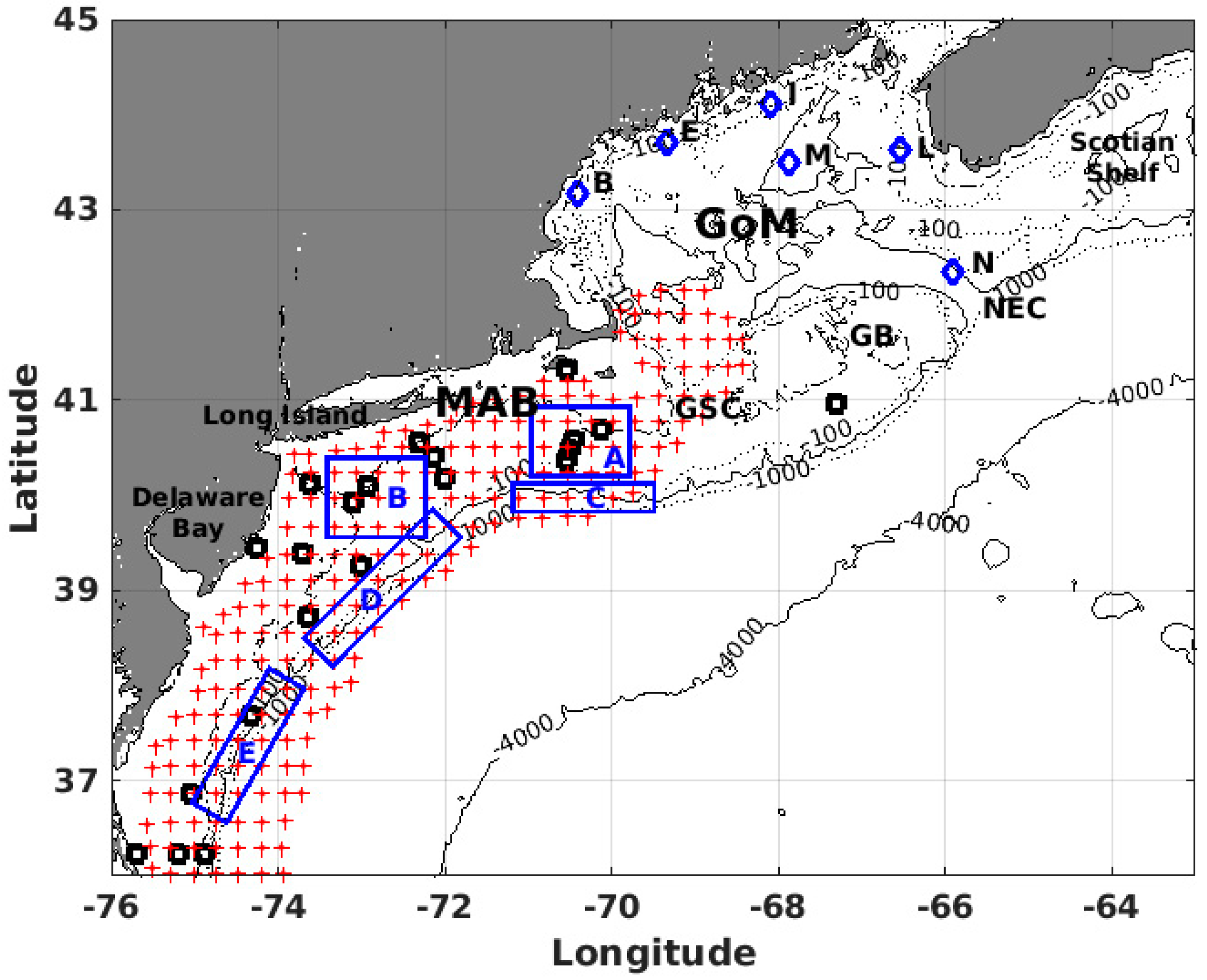
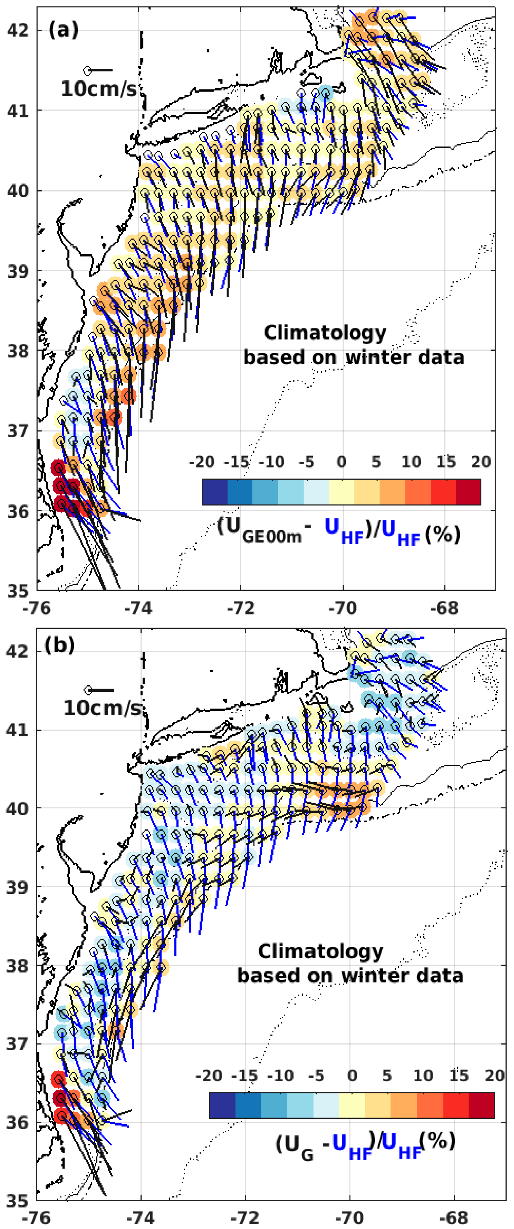
Figure 1.
Map of study region showing a set of in situ current measurement locations. Northeast Regional Association of Coastal Ocean Observing Systems (NERACOOS) moored Acoustic Doppler Current Profilers (ADCP) current buoys are in GoM (blue diamonds). In MAB the sites (black circles) of the in situ depth-average mean current dataset by Lentz [26] are shown as well as coastal ocean dynamics applications radar (CODAR) high frequency (HF) Radar current observations (red pluses) from Mid-Atlantic Regional Coastal Ocean Observing System (MARACOOS). Key geographic locations are noted, including the Scotian Shelf, Gulf of Maine (GoM), Northeast channel (NEC), Georges Bank (GB), Great South Channel (GSC), and Mid Atlantic Bight (MAB). Five selected analysis focus areas (blue boxes) in the MAB are labeled (A–E). Contours are for the 50-, 100- 1000-, and 4000-m isobaths.

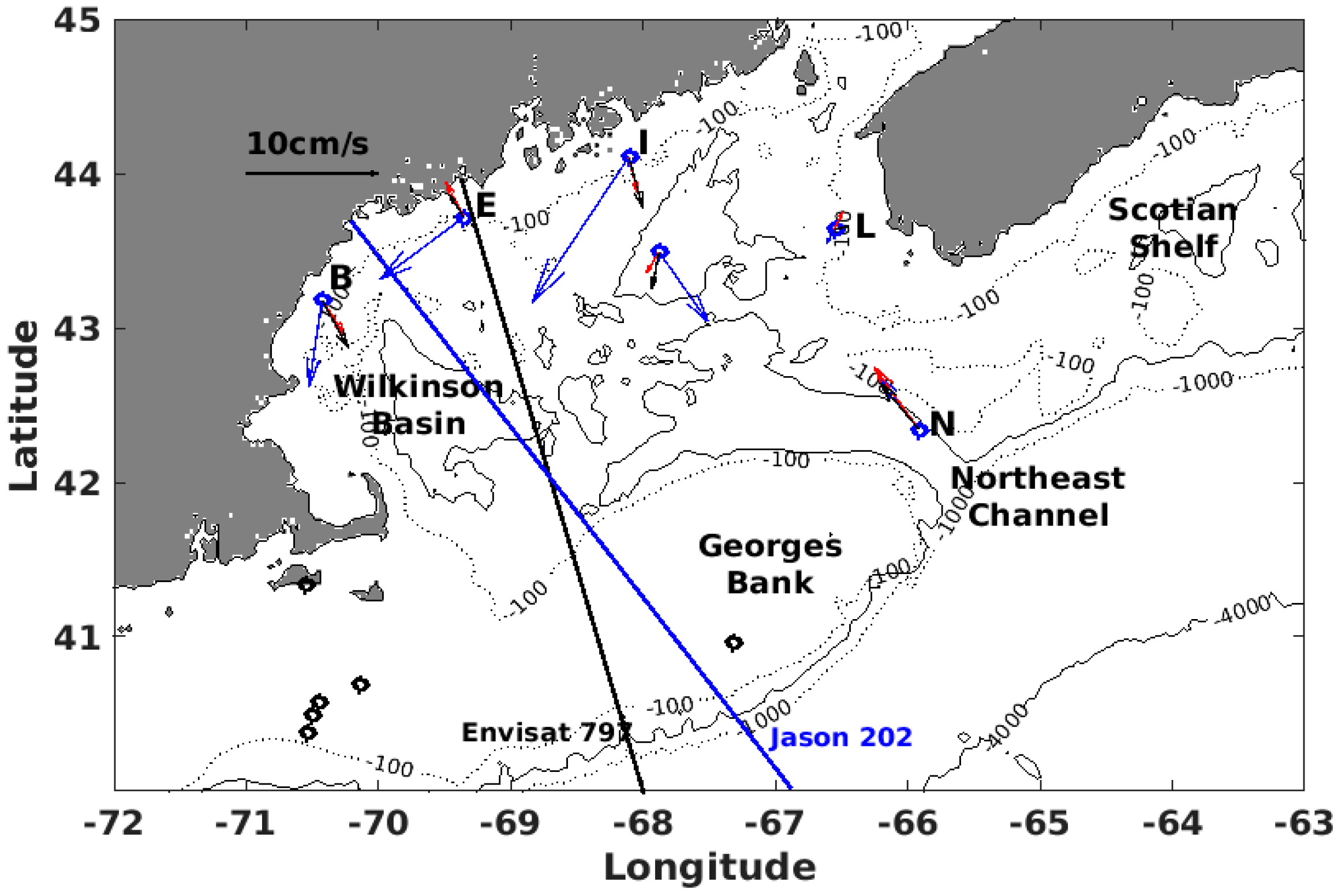
Figure 2.
Mean upper ocean current vectors for both in situ ADCP current measurements and GlobCurrent products on the Northwest Atlantic shelf in the GoM. In situ data are depth-averaged mean current vectors UDA15m in blue while GlobCurrent vector currents UG (Geostrophic only) are in red and UGE15m (Geostrophic and 15 m Ekman) are in black. Two satellite altimeter tracks (Envisat track E797, Jason track J202) are also shown.

Figure 3.
Derived mean dynamic topography (MDT) along (a) Envisat track E797 and (b) Jason track J202 from the western GoM across Georges Bank into the Atlantic slope region (Figure 2). Differing MDT estimates (see text) come from Mean Sea Surface (MSS) minus Geoid (G), either using MSSDTU [6] or MSSCLS [3] as well as from MDTAVISO [4] and MDTRU [48]. Grey areas depict the schematic bathymetry along these tracks. Note that the vertical offset between MDTRU and MDTAVISO is a matter of vertical datum but does not impact ocean dynamics.

Figure 4.
(a) GoM Buoy-N low-passed (70-day running mean applied) time series of current components of GC UG (Geostrophic) and UGE15 m (Geostrophic + 15 m Ekman) as well as ADCP depth-averaged (10–20 m) UDA15 m with upper and lower panels representing eastward u and northward v current components. Each panel provides statistical measures for UG vs. UDA15m (red text) and for UGE15m vs. UDA15m (black text). (b) Buoy-I low-passed time series in the same format.

Figure 5.
Statistics measures of R, RMSE, and Bias (top to bottom) between GlobCurrent and in situ ADCP depth-averaged (10–20 m) UDA15m current for (a) the eastward component (u) and (b) the northward component (v) at Buoys N, L, M, I, E and B labeled in X-axis in the GoM (see Figure 1). Results given for both UG (Geostrophic only) vs. UDA15m (grey) and UGE15m (Geostrophic and 15 m Ekman) vs. UDA15m (black).

Figure 6.
Mean upper ocean current vectors for both in situ current measurements and GlobCurrent products in the MAB on the Northwest Atlantic shelf. In situ data are depth-averaged current vectors UDA from Lentz [26] in blue while GlobCurrent vector currents UG (Geostrophic) and UGE15m (Geostrophic and 15 m Ekman) are in red and black, respectively.

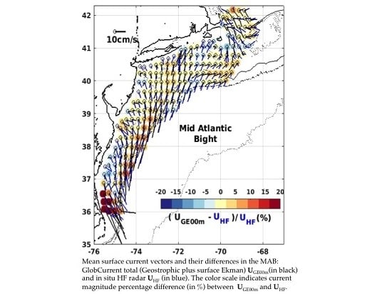
Figure 7.
Graphical display of mean surface current vectors and their differences in the MAB: (a) GlobCurrent UGE00m (b) GlobCurrent UG (in black) and in situ HF radar UHF (in blue). The color scale indicates current magnitude percentage difference (in %) between (a) UGE00m, (b) UG and UHF. The 50-, 100-, 1000- and 4000-m isobath contours are also shown. Calculations are based on year-round data during the shared sampling time period from 2006 to 2016.


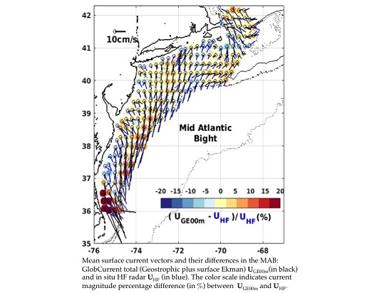
Figure 8.
Same caption text as in Figure 7, but calculations are based on the winter data (December, January, and February).
Figure 8.
Same caption text as in Figure 7, but calculations are based on the winter data (December, January, and February).

Figure 9.
MAB low-passed (70-days running mean applied) time series of alongshelf current u’ component for in situ HF radar u’HF (blue), GlobCurrent u’GE00m (black) and u’G (red) for the selected focus areas A–E (see Figure 1) shown from top to bottom. Each panel provides statistical measures for u’GE00m vs. u’HF (black text) and for u’G vs. u’HF (red text).

Figure 10.
Statistical measures of R, RMSE, and Bias (top to bottom) between MAB GlobCurrent and in situ HF radar UHF data for (a) the eastward component and (b) the northward component at the selected focus areas A-E labeled in X-axis (see Figure 1). Results given for both GC UG vs. UHF (in gray) and UGE00m vs. UHF (in black).


Table 1.
Summary of mean current speed and direction measurements at the specified in situ current meter locations (Figure 1). In situ data are depth-averaged mean current vectors UDA while GlobCurrent data products UG (Geostrophic only) and UGE15m (Geostrophic and 15 m Ekman) are the prescribed upper ocean (15 m) current estimates.
| Lat | Lon | UDA | UG | UGE | Buoy ID | |||
|---|---|---|---|---|---|---|---|---|
| 1 |UDA| | 2 ϕ | |UG| | ϕ | |UGE15m| | ϕ | |||
| (cm/s) (deg) | (cm/s) (deg) | (cm/s) (deg) | ||||||
| 3 GoM | ||||||||
| 42.34 | −65.92 | 4.4 | 131 | 5.2 | 130 | 4.2 | 134 | N |
| 43.64 | −66.55 | 1.1 | −125 | 1.3 | 61 | 1.1 | 10 | L |
| 43.49 | −67.88 | 5.9 | −51 | 1.7 | −126 | 2.4 | −103 | M |
| 44.11 | −68.11 | 11.9 | −128 | 2.5 | −74 | 3.5 | −72 | I |
| 43.72 | −69.36 | 7.5 | −148 | 2.6 | 121 | 1.8 | 127 | E |
| 43.18 | −70.43 | 5.7 | −100 | 2.9 | −53 | 3.7 | −57 | B |
| 4 MAB | ||||||||
| 40.97 | −67.32 | 9.1 | −160 | 8.7 | –146 | 9.2 | −139 | |
| 40.58 | −70.46 | 5.1 | 180 | 5.9 | 164 | 5.4 | 174 | |
| 40.49 | −70.51 | 7.6 | 180 | 7.6 | 168 | 7.2 | 176 | |
| 40.38 | −70.54 | 8.4 | 180 | 9.9 | 171 | 9.5 | 177 | |
| 40.69 | −70.14 | 5.0 | 158 | 6.1 | 174 | 5.8 | −176 | |
| 38.73 | −73.65 | 6.5 | −133 | 8.3 | –123 | 9.1 | −118 | |
| 37.70 | −74.34 | 8.7 | −126 | 12.4 | –115 | 13.2 | −113 | |
| 36.24 | −75.71 | 6.5 | −73 | 26.8 | −44 | 27.4 | −45 | |
| 36.24 | −75.21 | 3.1 | −76 | 18.8 | −57 | 19.5 | −59 | |
| 36.24 | −74.91 | 6.3 | −95 | 11.0 | −79 | 11.9 | −80 | |
| 36.87 | −75.05 | 4.5 | −76 | 6.6 | –167 | 6.8 | −160 | |
| 40.57 | −72.31 | 4.2 | −143 | 6.6 | –133 | 7.1 | −126 | |
| 40.42 | −72.14 | 3.2 | −144 | 5.5 | –127 | 6.1 | −119 | |
| 40.18 | −72.00 | 6.4 | −139 | 6.1 | –145 | 6.5 | −136 | |
| 40.11 | −72.92 | 2.0 | −113 | 3.1 | –139 | 3.5 | −125 | |
| 40.12 | −73.63 | 6.2 | 156 | 2.1 | 174 | 1.9 | −163 | |
| 39.93 | −73.10 | 5.4 | 179 | 3.2 | –154 | 3.5 | −138 | |
| 39.26 | −73.02 | 7.8 | −124 | 9.0 | –131 | 9.6 | −126 | |
| 39.41 | −73.72 | 2.8 | −113 | 2.2 | −70 | 3.1 | −71 | |
1: |U| mean speed (cm/s). 2: ϕ: mean velocity direction [−180, +180] clockwise and anticlockwise around the east. 3: UDA is the depth averaged (10–20 m) velocities UDA15m based on ADCP data at the GoM buoys. 4: UDA is the depth averaged mean velocities based on the MAB in situ dataset from Lentz [26].
Table 2.
Summary of GoM region statistical measure comparisons between components (eastward u and northward v) of in situ ADCP depth-averaged current velocities UDA15m and either GlobCurrent UG (Geostrophic only) or UGE15m (Geostrophic + 15 m Ekman) data. Also shown are standard deviations of these components for UDA15m, UG, and UGE15m. Analysis time periods differ for the separate buoy sites N, L, M, I, E and B, all exceeding 10 years except for site L. All data were low pass filtered with a 70-days running mean. N is number of observations.
| Buoy | R | RMSE (cm/s) | BIAS (cm/s) | Standard Deviation (cm/s) | N | ||||||||||||||
|---|---|---|---|---|---|---|---|---|---|---|---|---|---|---|---|---|---|---|---|
| UG | UGE15m | UG | UGE15m | UG | UGE | UDA15m | UG | UGE15m | |||||||||||
| u | v | u | v | u | v | u | v | u | v | u | v | u | v | u | v | u | v | ||
| N | 0.77 | 0.46 | 0.78 | 0.53 | 3.4 | 4.4 | 3.4 | 4.2 | −0.4 | 0.6 | 0.1 | −0.4 | 5.4 | 4.3 | 3.8 | 4.2 | 3.9 | 4.3 | 3647 |
| L | −0.08 | 0.03 | −0.09 | 0.05 | 4.1 | 5.6 | 3.9 | 5.6 | 1.5 | 3.1 | 2.1 | 2.2 | 1.6 | 3.4 | 3.7 | 4.5 | 3.4 | 4.6 | 1769 |
| M | 0.42 | 0.12 | 0.45 | 0.19 | 3.5 | 4.7 | 3.6 | 4.5 | −4.6 | 3.0 | −3.9 | 2.1 | 3.1 | 3.1 | 3.5 | 3.9 | 3.7 | 3.9 | 4143 |
| I | 0.37 | 0.37 | 0.30 | 0.28 | 4.4 | 3.9 | 4.6 | 4.0 | 8.1 | 7.0 | 8.8 | 6.1 | 4.4 | 2.5 | 3.3 | 4.1 | 3.2 | 3.9 | 4832 |
| E | 0.35 | −0.05 | 0.31 | 0.10 | 4.0 | 4.0 | 4.1 | 3.9 | 4.9 | 6.4 | 5.4 | 5.7 | 4.1 | 2.0 | 2.6 | 3.4 | 2.6 | 3.5 | 4932 |
| B | 0.13 | −0.18 | 0.17 | −0.24 | 2.6 | 4.9 | 2.5 | 5.1 | 2.7 | 3.3 | 3.1 | 2.7 | 1.8 | 3.4 | 2.1 | 3.0 | 2.1 | 3.1 | 4846 |
Table 3.
MAB data in the same form as for Table 2. Statistical measure comparisons are now between collocated in situ CODAR HF radar measured current velocity UHF and either GlobCurrent UG (Geostrophic only) or UGE00m (Geostrophic + surface Ekman). Num is number of observations. The selected focus areas A–E in the MAB are shown as in Figure 1.
| R | RMSE (cm/s) | BIAS (cm/s) | Standard Deviation (cm/s) | Number | |||||||||||||||
|---|---|---|---|---|---|---|---|---|---|---|---|---|---|---|---|---|---|---|---|
| UG | UGE00m | UG | UGE00m | UG | UGE00m | UHF | UG | UGE00m | |||||||||||
| u | v | u | v | u | v | u | v | u | v | u | v | u | v | u | v | u | v | ||
| Area A | 0.47 | −0.09 | 0.74 | 0.22 | 2.8 | 2.7 | 2.3 | 3.0 | 5.1 | 4.5 | −2.5 | 2.5 | 2.9 | 2.3 | 2.5 | 1.2 | 3.3 | 2.6 | 2770 |
| Area B | 0.60 | 0.21 | 0.81 | 0.48 | 1.7 | 2.7 | 1.7 | 2.1 | 5.7 | 2.0 | −2.8 | 0.4 | 2.1 | 1.7 | 1.5 | 2.5 | 2.8 | 2.2 | 3482 |
| Area C | 0.56 | 0.16 | 0.65 | 0.35 | 6.0 | 3.1 | 5.3 | 3.4 | 5.1 | 4.8 | −2.2 | 2.3 | 5.0 | 3.0 | 7.1 | 1.4 | 7.0 | 3.0 | 2073 |
| Area D | 0.70 | 0.56 | 0.81 | 0.71 | 2.6 | 2.8 | 2.5 | 3.3 | 6.3 | 1.0 | −3.2 | −1.6 | 3.5 | 2.6 | 3.2 | 3.3 | 4.2 | 4.6 | 2959 |
| Area E | 0.47 | 0.76 | 0.57 | 0.83 | 3.0 | 3.6 | 3.0 | 3.9 | 6.8 | −3.3 | −4.4 | −4.8 | 3.4 | 3.9 | 1.7 | 5.5 | 3.0 | 6.5 | 3020 |
© 2018 by the authors. Licensee MDPI, Basel, Switzerland. This article is an open access article distributed under the terms and conditions of the Creative Commons Attribution (CC BY) license (http://creativecommons.org/licenses/by/4.0/).
Share and Cite
MDPI and ACS Style
Feng, H.; Vandemark, D.; Levin, J.; Wilkin, J. Examining the Accuracy of GlobCurrent Upper Ocean Velocity Data Products on the Northwestern Atlantic Shelf. Remote Sens. 2018, 10, 1205. https://doi.org/10.3390/rs10081205
AMA Style
Feng H, Vandemark D, Levin J, Wilkin J. Examining the Accuracy of GlobCurrent Upper Ocean Velocity Data Products on the Northwestern Atlantic Shelf. Remote Sensing. 2018; 10(8):1205. https://doi.org/10.3390/rs10081205
Chicago/Turabian StyleFeng, Hui, Douglas Vandemark, Julia Levin, and John Wilkin. 2018. "Examining the Accuracy of GlobCurrent Upper Ocean Velocity Data Products on the Northwestern Atlantic Shelf" Remote Sensing 10, no. 8: 1205. https://doi.org/10.3390/rs10081205
Note that from the first issue of 2016, this journal uses article numbers instead of page numbers. See further details here.