Figure 1.
(
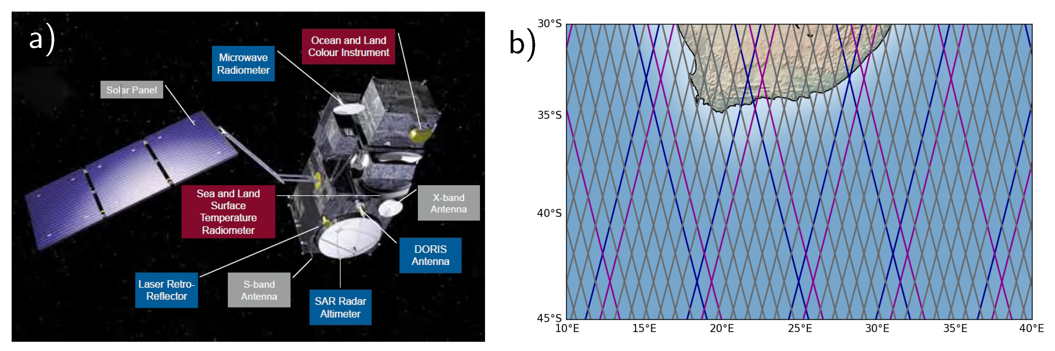
a) Illustration of Sentinel-3 spacecraft showing most of the equipment payload (image courtesy of ESA). (
b) Example of track pattern (all lines) surveyed by Sentinel-3A in 27 days in the Agulhas region, South Africa. Blue lines show the nearly uniform coarser coverage from a 4-day period (sub-cycle), with magenta lines showing the subsequent 4 days. [Left-hand figure taken from [
2]].
Figure 1.
(
a) Illustration of Sentinel-3 spacecraft showing most of the equipment payload (image courtesy of ESA). (
b) Example of track pattern (all lines) surveyed by Sentinel-3A in 27 days in the Agulhas region, South Africa. Blue lines show the nearly uniform coarser coverage from a 4-day period (sub-cycle), with magenta lines showing the subsequent 4 days. [Left-hand figure taken from [
2]].
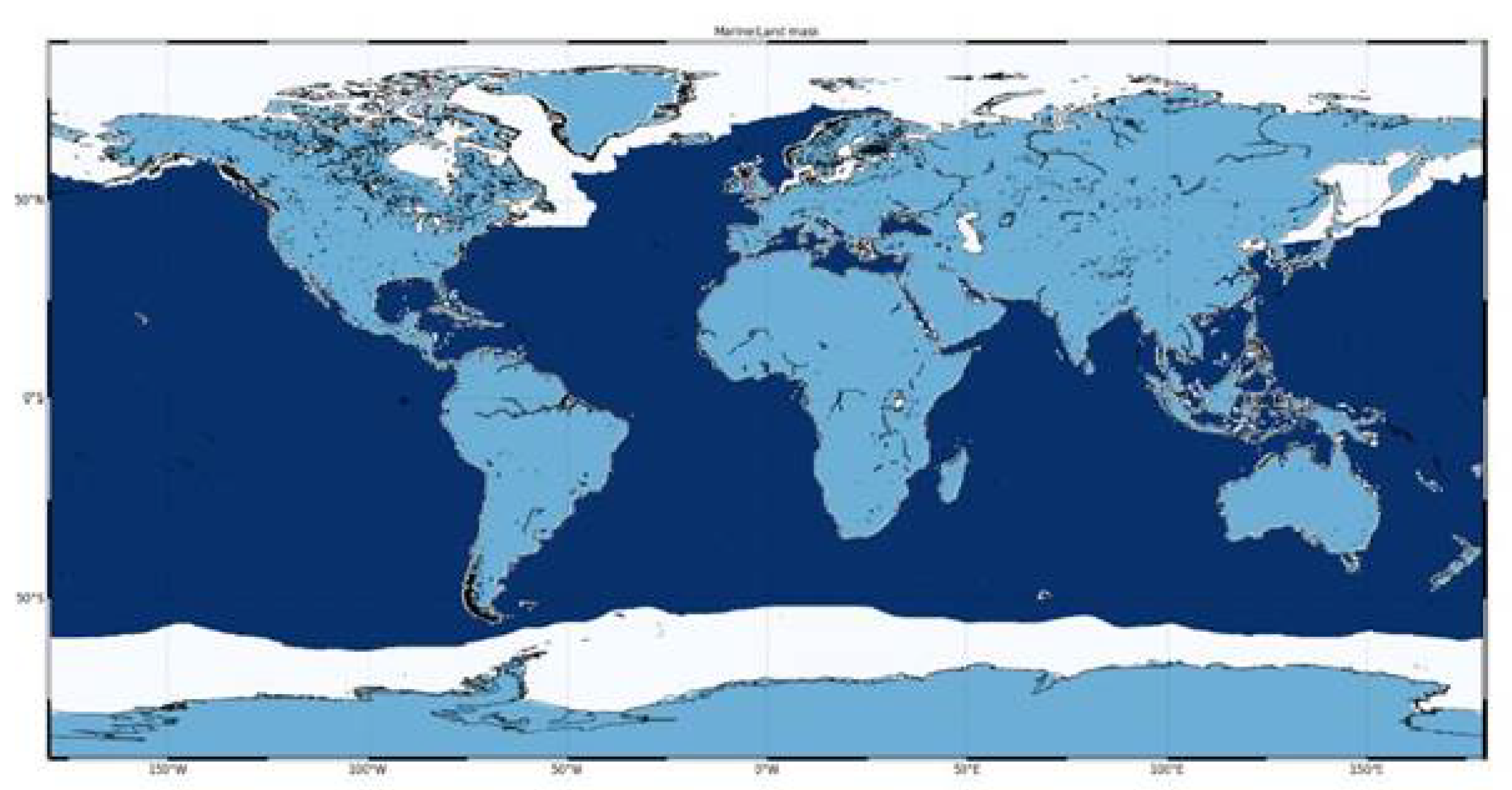
Figure 2.
Land/Sea mask showing the regions of responsibility for data production for mid 2020 onwards (expected). Data over land (light blue) are produced and disseminated by ESA; those over the ocean (dark blue) by EUMETSAT; some regions (white) are common to both, including the polar regions of maximal sea-ice extent and major inland water bodies (e.g., Caspian Sea, Great Lakes, Lake Victoria). As users for terrestrial data may benefit from the records just offshore, and those working in the coastal zone benefit from having the data just inland, these regions extend 25 km outward/inward from the coast to avoid researchers needing to gather data from two sources.
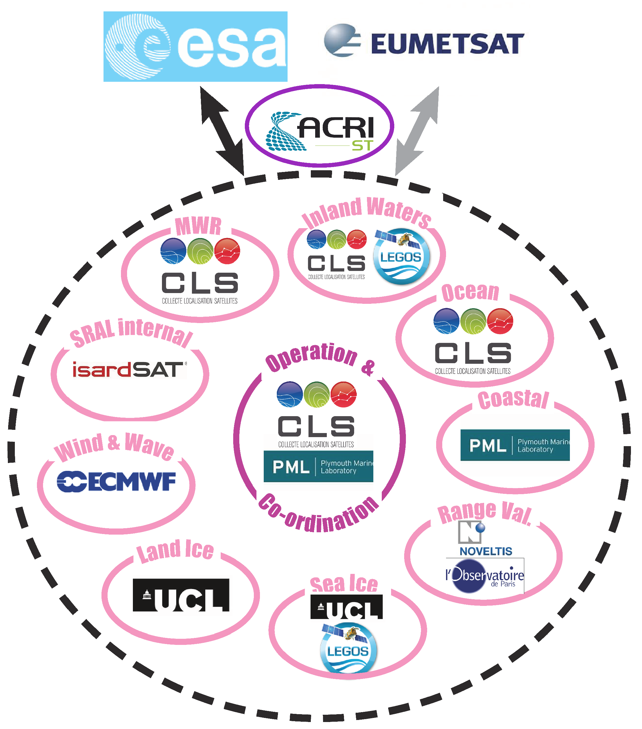
Figure 3.
Organigram showing the areas of expertise of the various Expert Support Laboratories within the STM component of the S3MPC, and their interaction with ESA and EUMETSAT. Overall management of the S3MPC contract is provided by ACRI-ST.
Figure 3.
Organigram showing the areas of expertise of the various Expert Support Laboratories within the STM component of the S3MPC, and their interaction with ESA and EUMETSAT. Overall management of the S3MPC contract is provided by ACRI-ST.
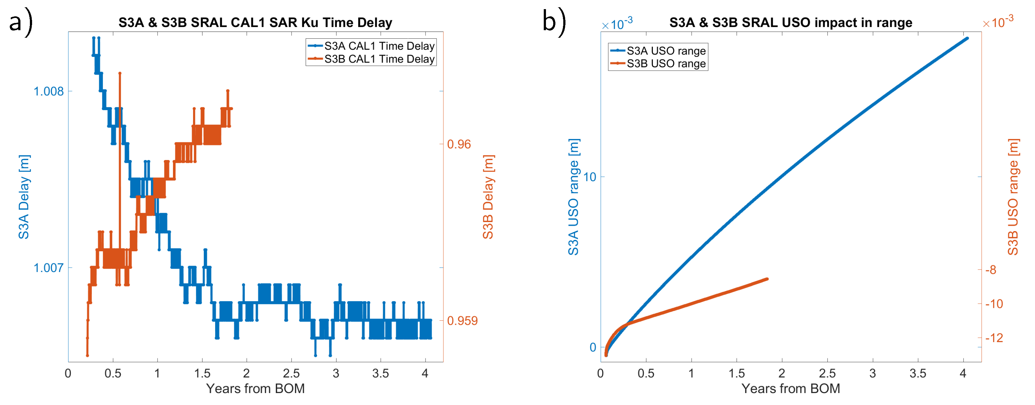
Figure 4.
S3A and S3B whole mission series of calibration parameters correcting science range measurements: (a) calibration path time delay, and (b) range delay due to not-nominal Ultra-Stable Oscillator frequency.
Figure 4.
S3A and S3B whole mission series of calibration parameters correcting science range measurements: (a) calibration path time delay, and (b) range delay due to not-nominal Ultra-Stable Oscillator frequency.
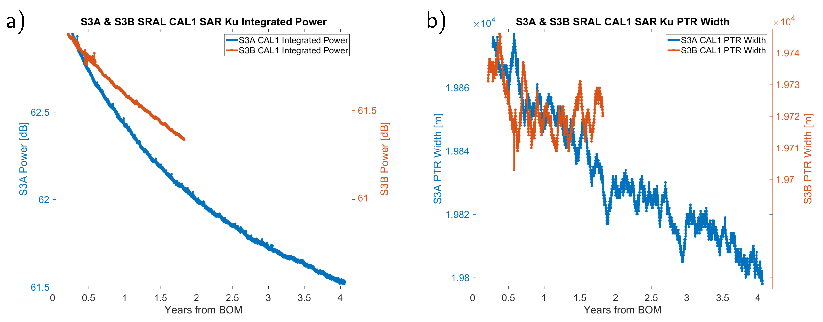
Figure 5.
Complete mission series of S3A and S3B SRAL instrumental corrections for (a) emitted power, and (b) CAL1 PTR width.
Figure 5.
Complete mission series of S3A and S3B SRAL instrumental corrections for (a) emitted power, and (b) CAL1 PTR width.
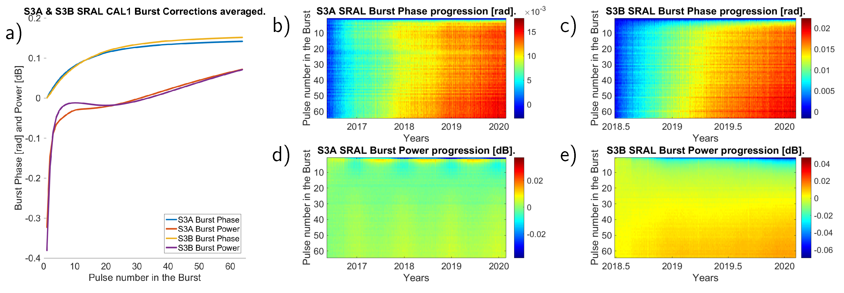
Figure 6.
Complete mission averaged CAL1 Intra-burst correction of S3A and S3B: (a) averaged mission series, (b,d) S3A burst corrections progression with respect to first record, and (c,e) S3B burst corrections progression with respect to first record.
Figure 6.
Complete mission averaged CAL1 Intra-burst correction of S3A and S3B: (a) averaged mission series, (b,d) S3A burst corrections progression with respect to first record, and (c,e) S3B burst corrections progression with respect to first record.
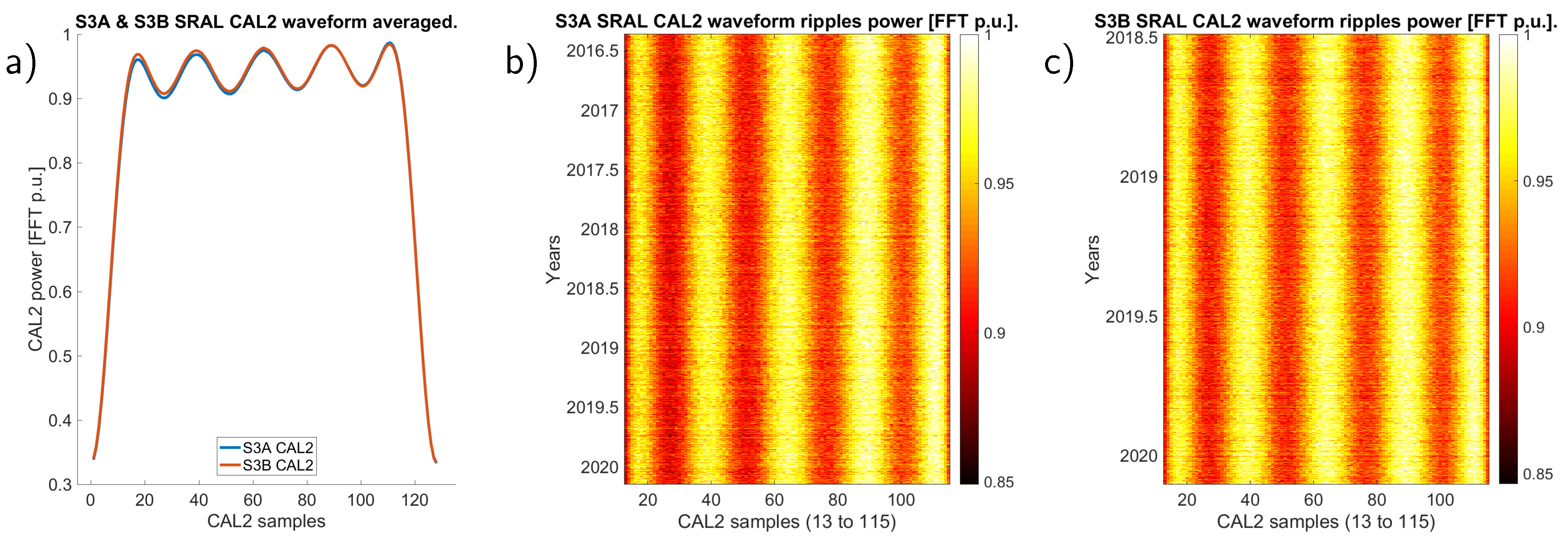
Figure 7.
CAL2 correction (in FFT power units) of S3A and S3B missions: (a) averaged mission Transfer Function, (b) S3A CAL2 ripples progression, and (c) S3B CAL2 ripples progression.
Figure 7.
CAL2 correction (in FFT power units) of S3A and S3B missions: (a) averaged mission Transfer Function, (b) S3A CAL2 ripples progression, and (c) S3B CAL2 ripples progression.
Figure 8.
AutoCal correction of S3A and S3B missions: (a) averaged mission attenuation (measured minus reference), (b) S3A attenuations progression with respect to first record, and (c) S3B attenuations progression with respect to first record.
Figure 8.
AutoCal correction of S3A and S3B missions: (a) averaged mission attenuation (measured minus reference), (b) S3A attenuations progression with respect to first record, and (c) S3B attenuations progression with respect to first record.
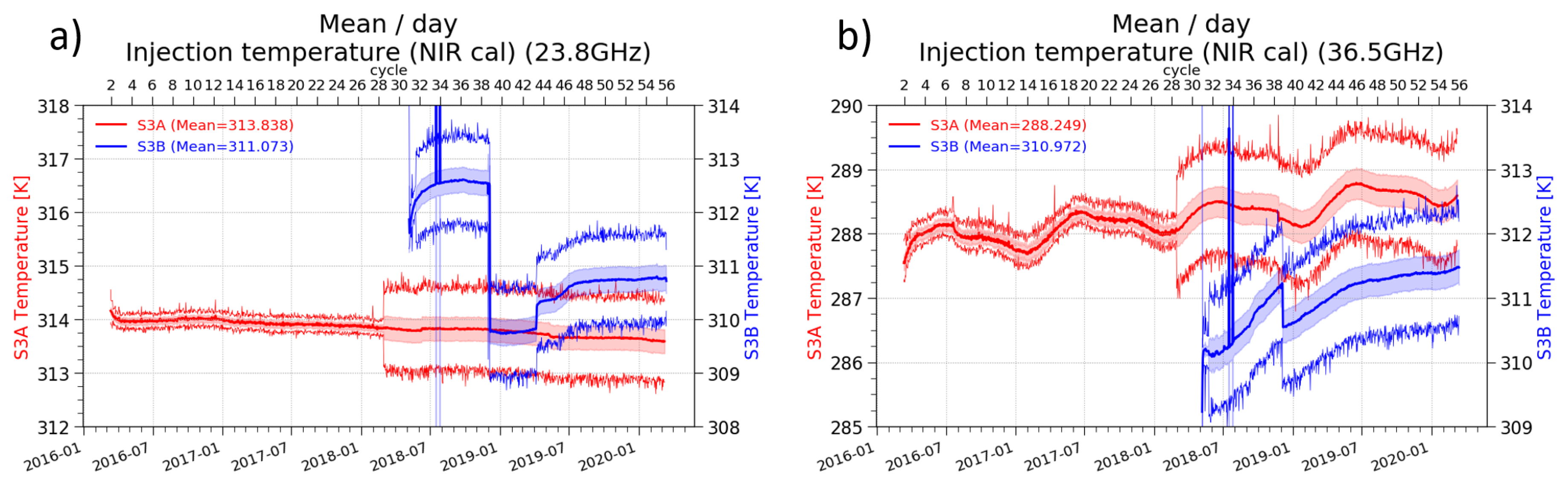
Figure 9.
Daily noise injection temperatures for S3A (red) and S3B (blue). Bold lines show the average, shades the standard deviation and lighter lines are minimum/maximum values. (a) 23.8 GHz channel (b) 36.5 GHz channel.
Figure 9.
Daily noise injection temperatures for S3A (red) and S3B (blue). Bold lines show the average, shades the standard deviation and lighter lines are minimum/maximum values. (a) 23.8 GHz channel (b) 36.5 GHz channel.
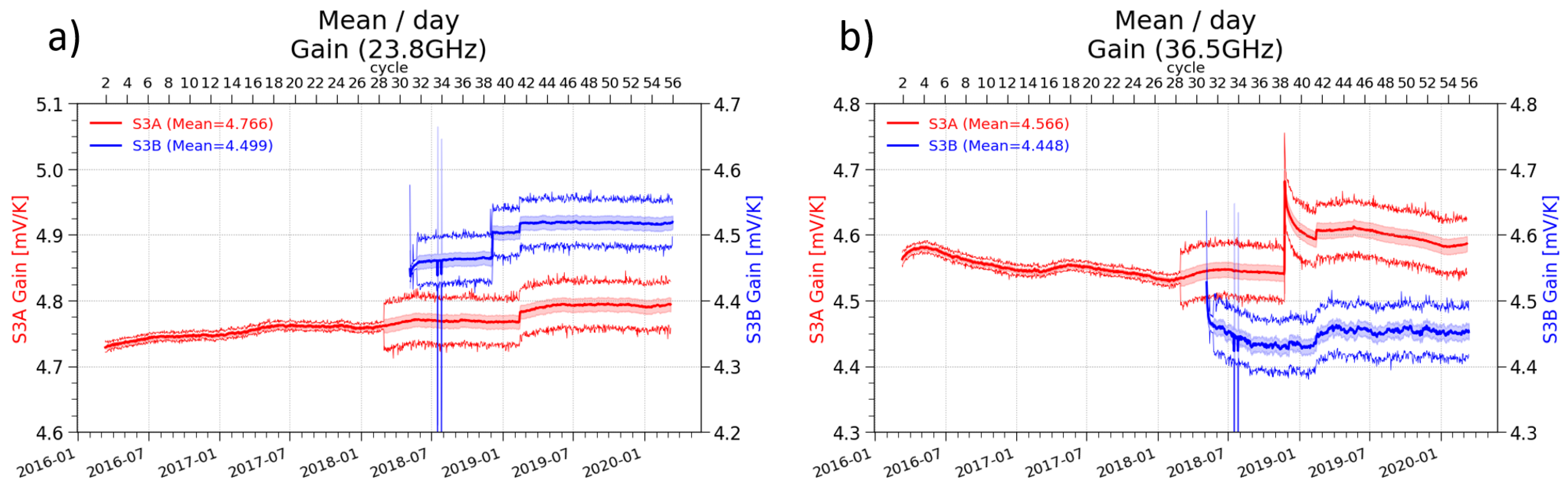
Figure 10.
Receiver gain for S3A (red) and S3B (blue). Bold lines show the average, shades the standard deviation and lighter lines are minimum/maximum values. (a) 23.8 GHz channel (b) 36.5 GHz channel.
Figure 10.
Receiver gain for S3A (red) and S3B (blue). Bold lines show the average, shades the standard deviation and lighter lines are minimum/maximum values. (a) 23.8 GHz channel (b) 36.5 GHz channel.
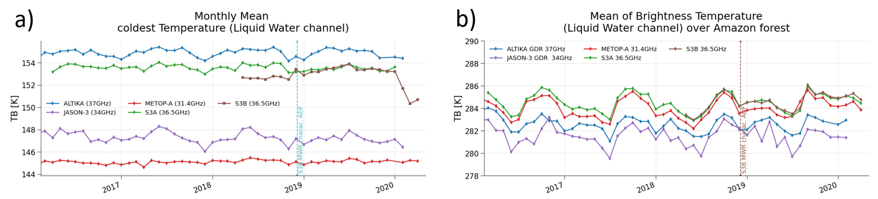
Figure 11.
Monitoring of (a) Cold reference and (b) Hot reference for 23.8 GHz channel of S3A and S3B.
Figure 11.
Monitoring of (a) Cold reference and (b) Hot reference for 23.8 GHz channel of S3A and S3B.
Figure 12.
Monitoring of (a) Cold reference and (b) Hot reference for 36.5 GHz channel of S3A and S3B.
Figure 12.
Monitoring of (a) Cold reference and (b) Hot reference for 36.5 GHz channel of S3A and S3B.
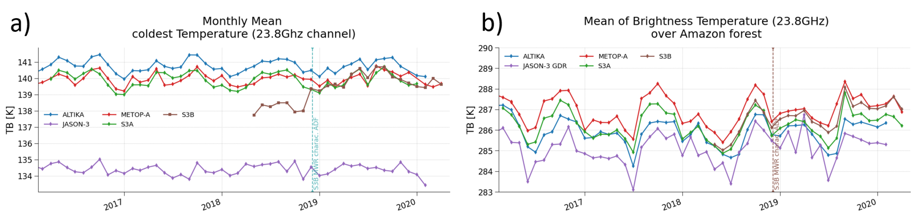
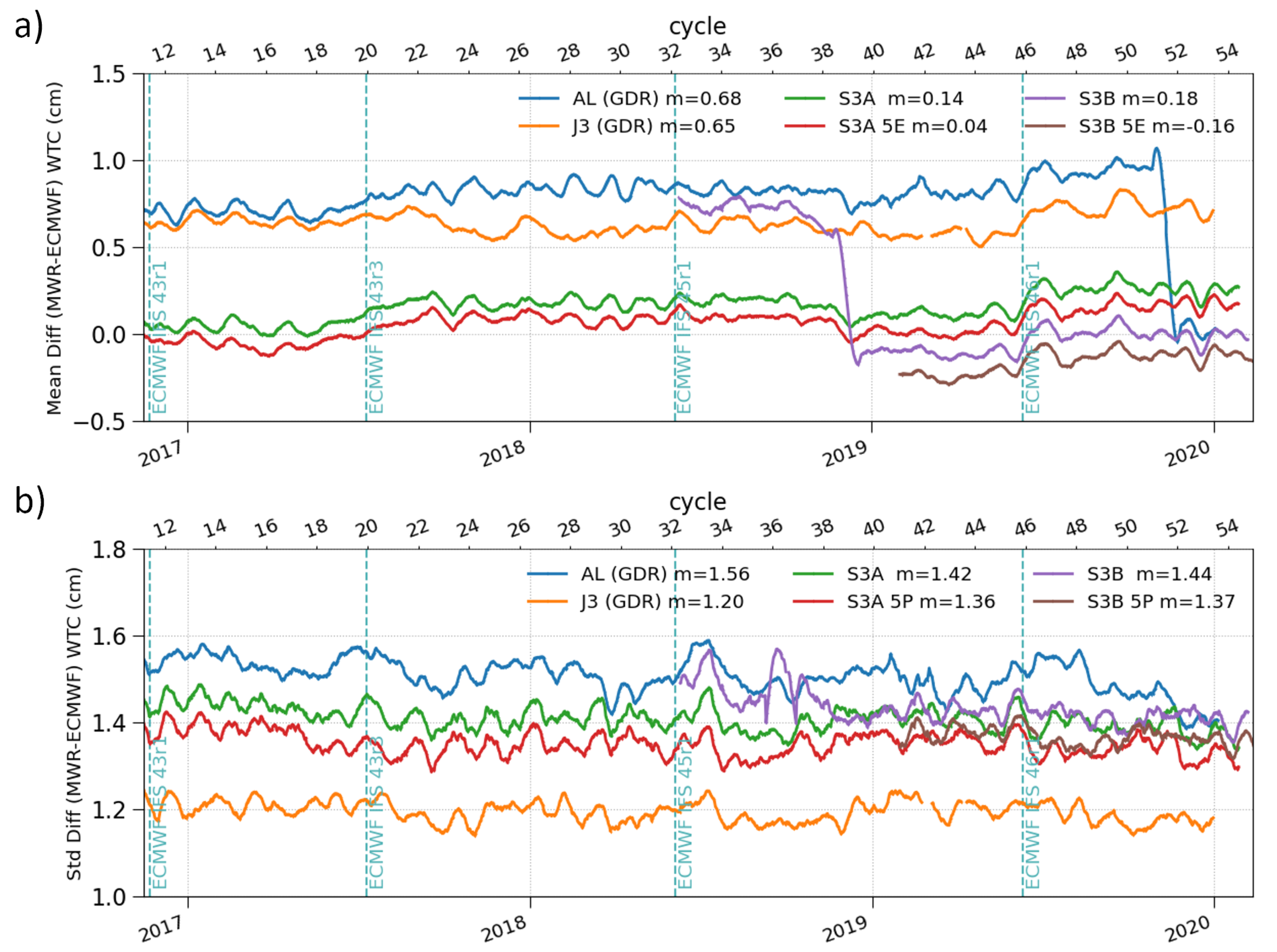
Figure 13.
Comparison of MWR-derived corrections with those from ECMWF model. (a) Mean WTC difference (b) S.D. WTC difference. The vertical lines in cyan indicate changes in the ECMWF operational model used as the reference. Note, there was an update to the S3B characterization file in Dec. 2018, and the default AltiKa algorithm changed from 3-parameter to 5-parameter in Dec. 2019.
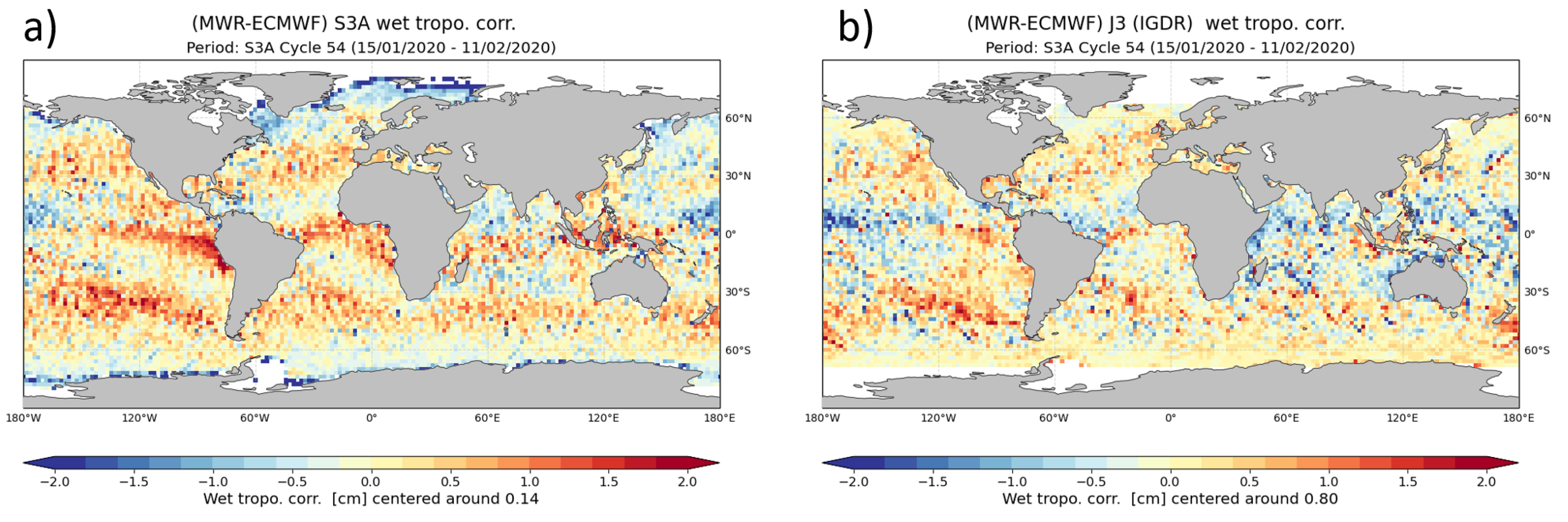
Figure 14.
Geographical variation of WTC bias (MWR-derived correction minus those from ECMWF model. (a) S3A, with a mean bias of 0.14 cm removed (b) Jason-3 MWR for the same period, with 0.80 cm removed.
Figure 14.
Geographical variation of WTC bias (MWR-derived correction minus those from ECMWF model. (a) S3A, with a mean bias of 0.14 cm removed (b) Jason-3 MWR for the same period, with 0.80 cm removed.
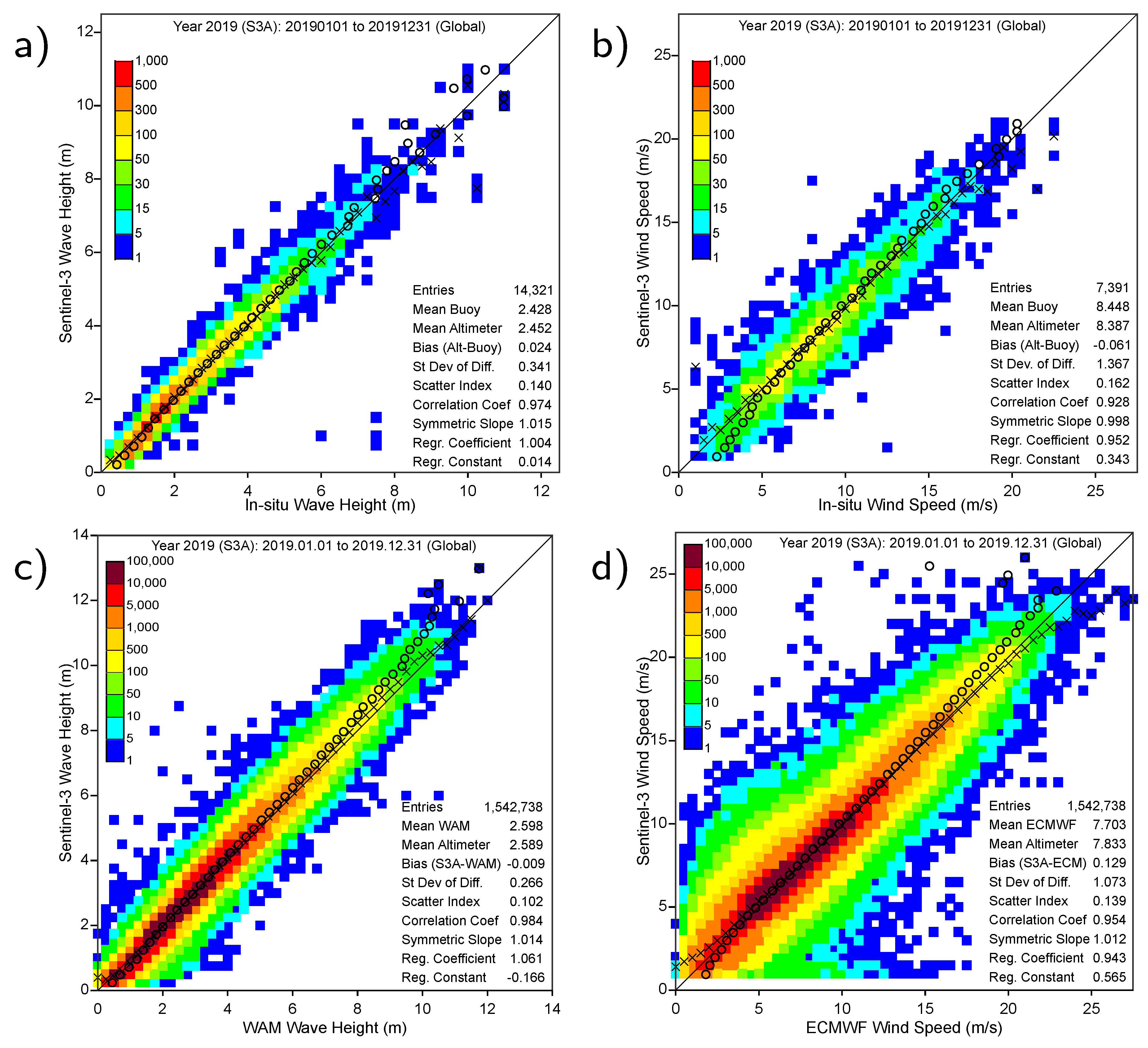
Figure 15.
Comparison of S3A Wind and Wave Data for whole of 2019. (a) Wave height from buoys (b) Wind speed from buoys (c) Wave height from ECMWF WAM model (first guess) (d) Wind speed from ECMWF model (analysis). Plots are 2-D histograms with intervals of 0.5 m/s for wind speed and 0.25 m for SWH; the ‘x’ symbols mark the mean value of altimeter for given in situ, and the ‘o’ symbols show the mean of the in situ for a given altimeter estimate.
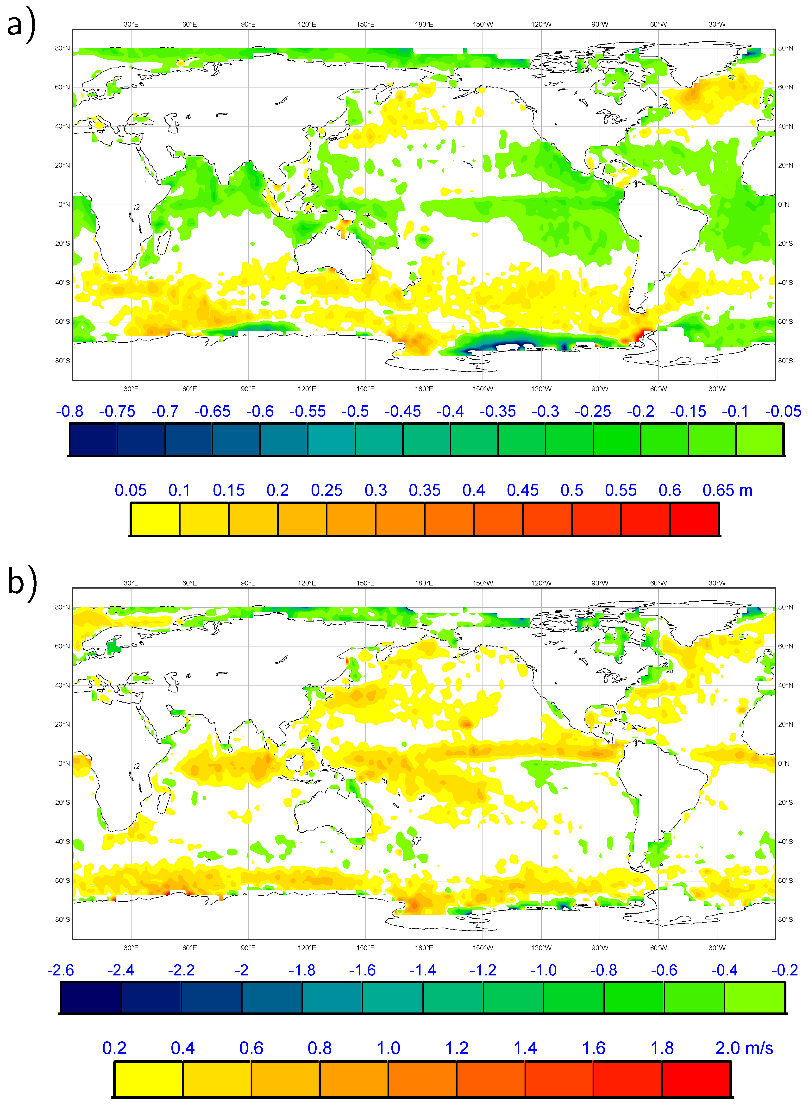
Figure 16.
Geographical variation in S3A bias with respect to a model. (a) Wave height (b) Wind speed.
Figure 16.
Geographical variation in S3A bias with respect to a model. (a) Wave height (b) Wind speed.
Figure 17.
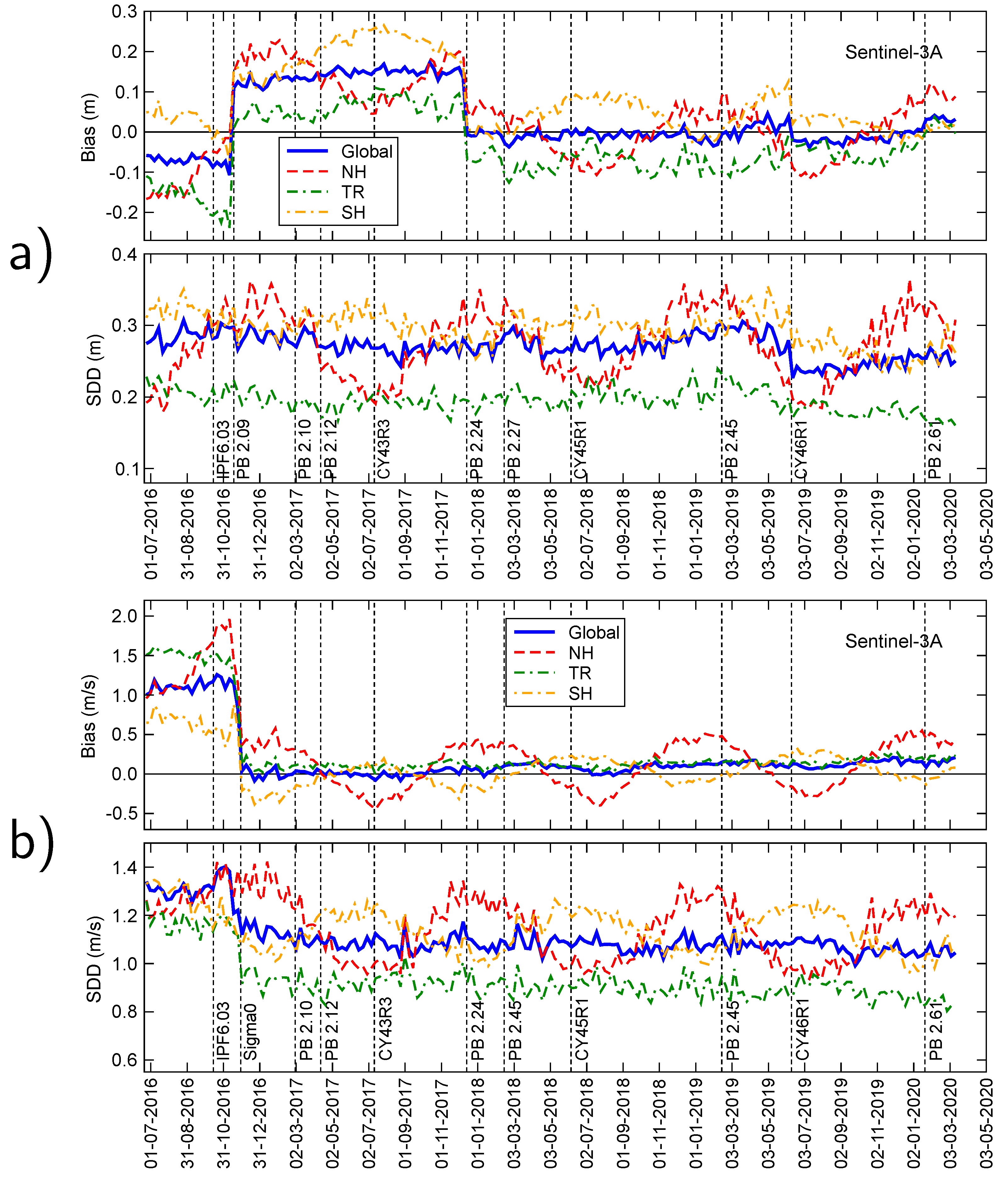
Time series showing evolution in S3A bias and SDD (Standard deviation of difference) with respect to a model, as different PBs are implemented in the NRT processing or changes made in the ECMWF model (indicated by ‘CY’). (a) Wave height (b) Wind speed. Data are plotted with a 7-day running mean, ‘NH’ is the northern hemisphere, north of 20N; ‘SH’ is south of 20S and ‘TR’ the tropical band in between.
Figure 17.
Time series showing evolution in S3A bias and SDD (Standard deviation of difference) with respect to a model, as different PBs are implemented in the NRT processing or changes made in the ECMWF model (indicated by ‘CY’). (a) Wave height (b) Wind speed. Data are plotted with a 7-day running mean, ‘NH’ is the northern hemisphere, north of 20N; ‘SH’ is south of 20S and ‘TR’ the tropical band in between.
Figure 18.
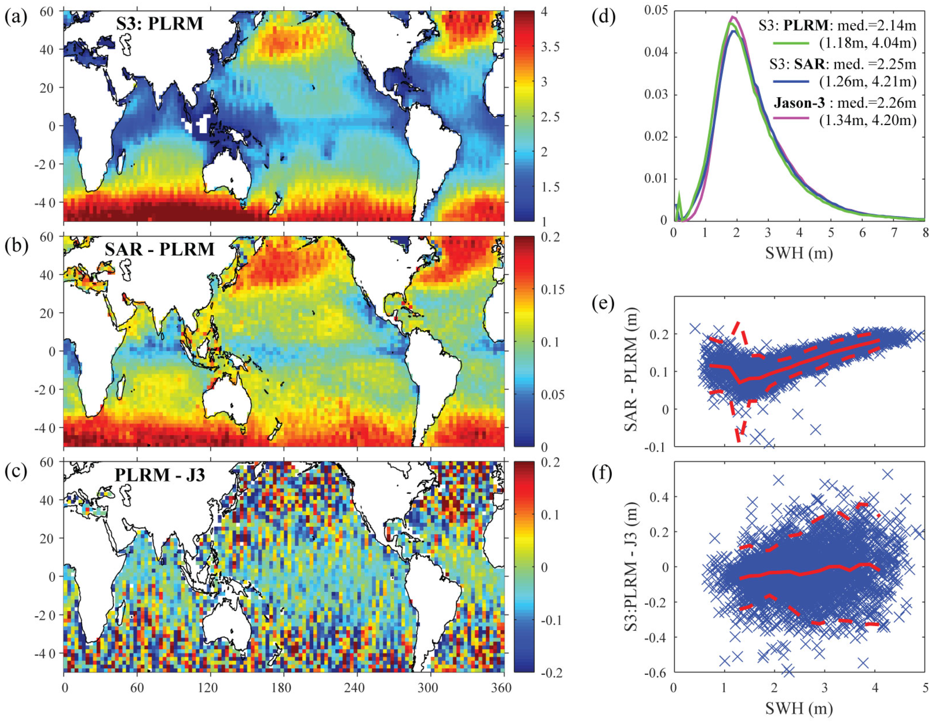
Comparison of altimeter SWH data for 2019. (a) Average of all 2019 for Sentinel-3 PLRM data (b) Mean bias of Sentinel-3 SAR mode data to those from PLRM (c) Difference of mean fields from S3:PLRM and Jason-3 (LRM) (d) Probability distribution functions of SWH data for Jan. 2019. Numerical values are the median and (in brackets) the 10th and 90th percentiles. Data are limited to 50S to 60N to avoid effects of undetected sea-ice. Comparison of grid box means for 2019 for (e) S3:SAR relative to PLRM and (f) PLRM relative to Jason-3. Full red lines show mean relationship in 0.2 m wide bins with the dashed lines showing ±2 std. dev. For these last 2 plots some data exist outside the axes shown, but these are relatively few.
Figure 18.
Comparison of altimeter SWH data for 2019. (a) Average of all 2019 for Sentinel-3 PLRM data (b) Mean bias of Sentinel-3 SAR mode data to those from PLRM (c) Difference of mean fields from S3:PLRM and Jason-3 (LRM) (d) Probability distribution functions of SWH data for Jan. 2019. Numerical values are the median and (in brackets) the 10th and 90th percentiles. Data are limited to 50S to 60N to avoid effects of undetected sea-ice. Comparison of grid box means for 2019 for (e) S3:SAR relative to PLRM and (f) PLRM relative to Jason-3. Full red lines show mean relationship in 0.2 m wide bins with the dashed lines showing ±2 std. dev. For these last 2 plots some data exist outside the axes shown, but these are relatively few.
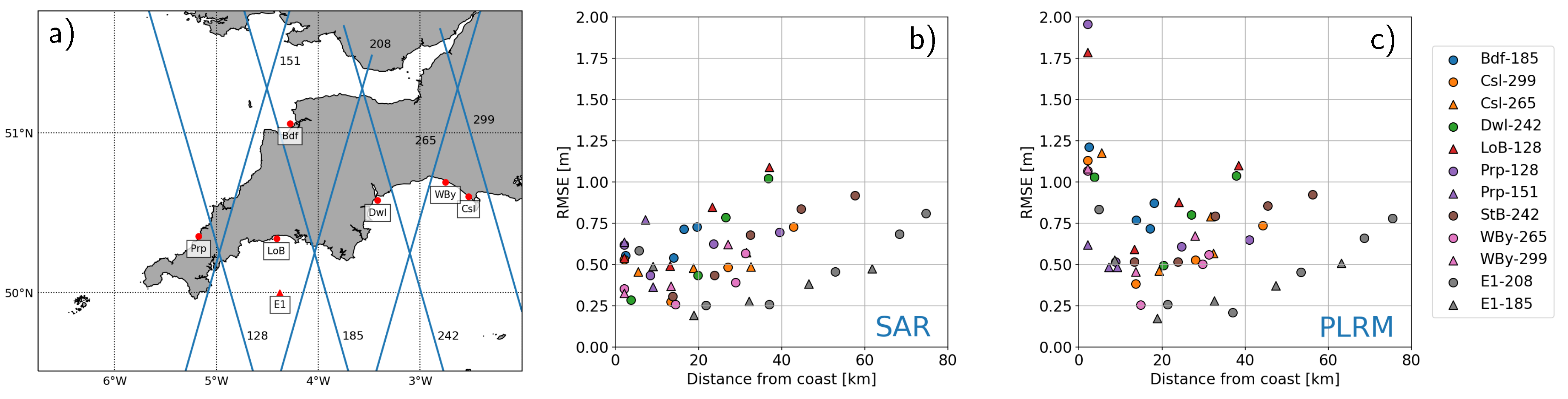
Figure 19.
(
a) Locations of the wave buoys and Sentinel-3A tracks around southwest UK used for the validation. Root mean square bias of S3A wave height and in situ coastal wave buoys observations as a function of distance to coast: (
b) SAR mode (
c) PLRM mode. (Each coloured symbol represents a different track-buoy comparison.). From Nencioli and Quartly [
33].
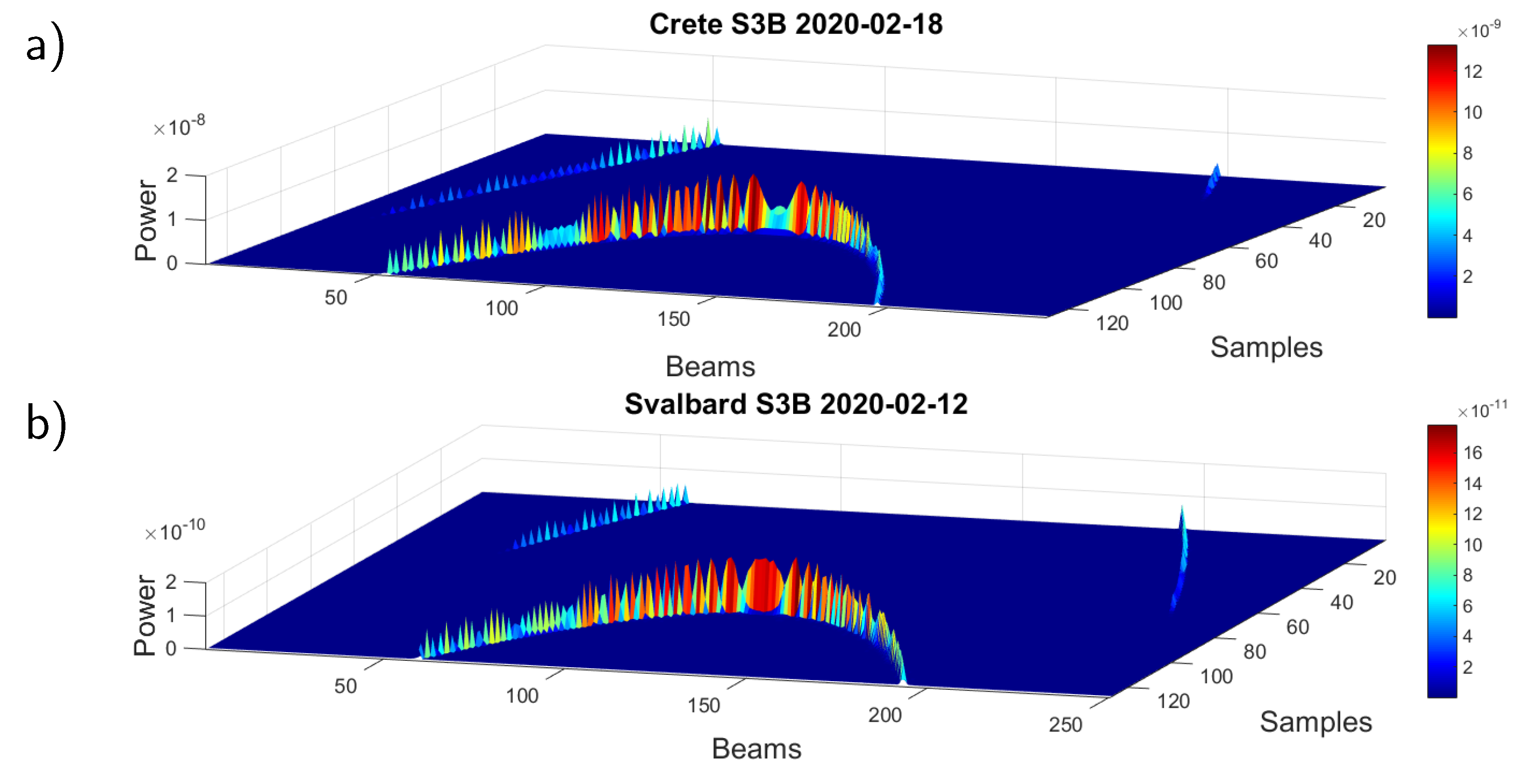
Figure 20.
Stack data for (a) Sentinel 3B pass (2020-02-18) over Crete and (b) Sentinel 3B pass (12 February 2020) over Svalbard.
Figure 20.
Stack data for (a) Sentinel 3B pass (2020-02-18) over Crete and (b) Sentinel 3B pass (12 February 2020) over Svalbard.
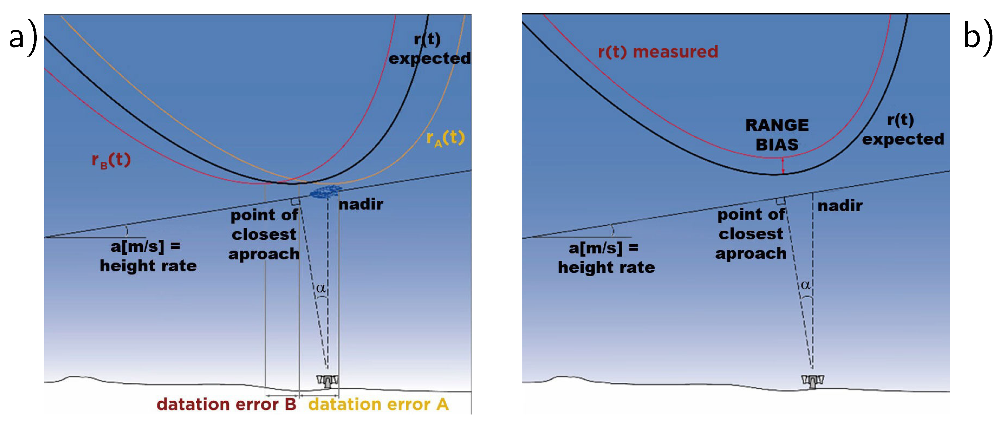
Figure 21.
Schematic showing the effect of errors on the sequence of observed ranges (shown by the range vs. time parabolae). (a) An error in datation (timing of observations) means that the apex appears to occur at a different position along track. (b) An error in range results in a parabola nearer to or further away than expected from the point of closest approach.
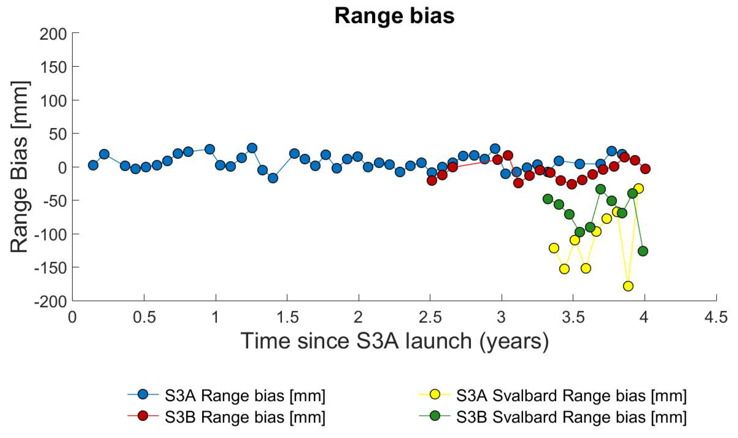
Figure 22.
Range bias results.
Figure 22.
Range bias results.
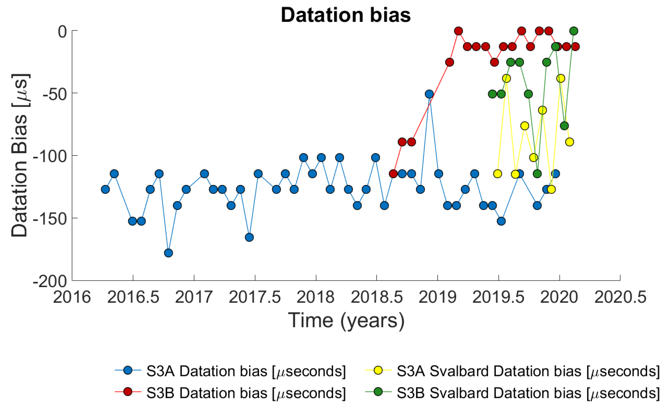
Figure 23.
Datation bias results.
Figure 23.
Datation bias results.
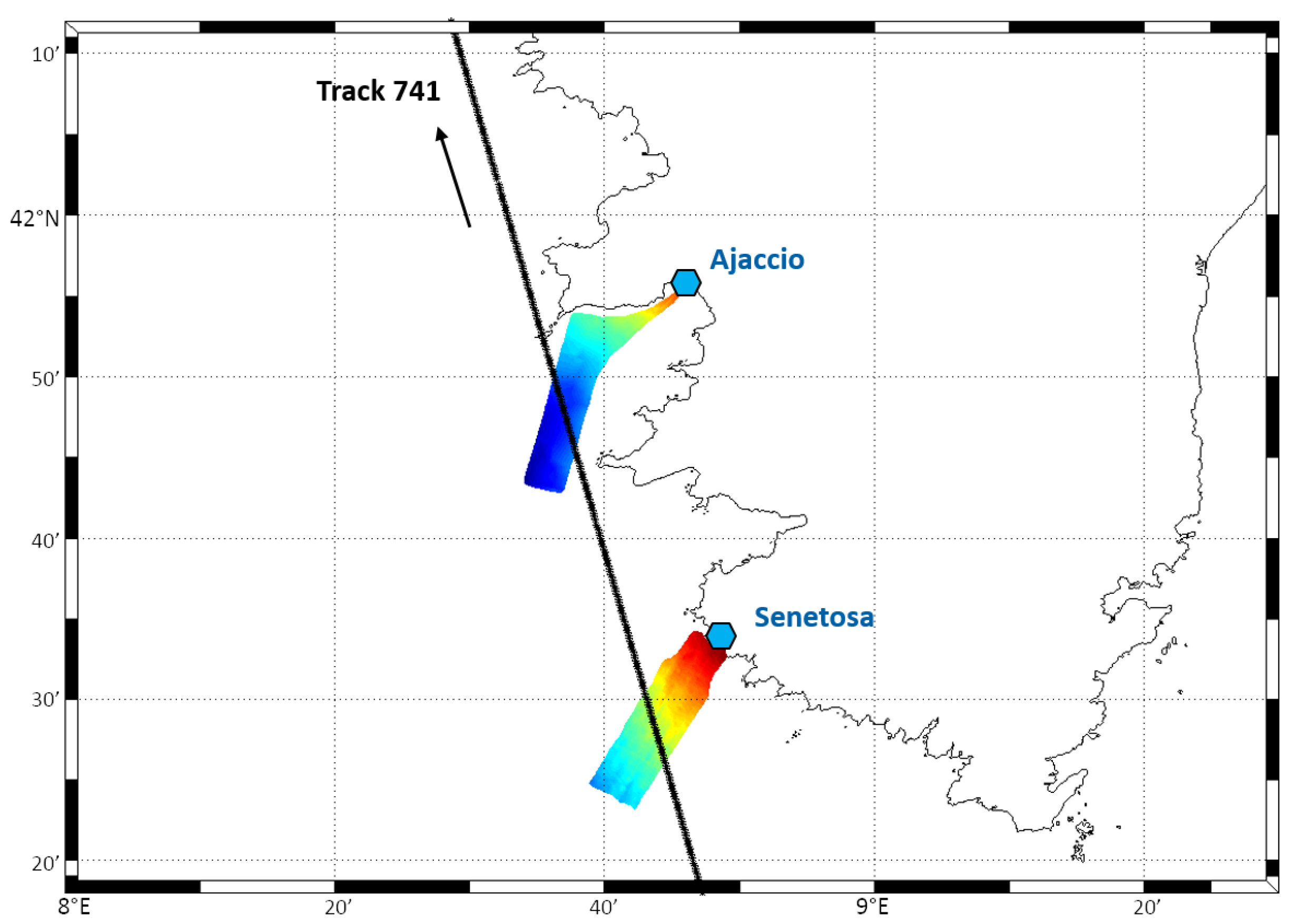
Figure 24.
Configuration for absolute calibration off Corsica. The regions in colours show the two high-resolution mean sea surfaces that were specifically measured by Bonnefond et al. [
41] to link the calibration sites to the altimetry data.
Figure 24.
Configuration for absolute calibration off Corsica. The regions in colours show the two high-resolution mean sea surfaces that were specifically measured by Bonnefond et al. [
41] to link the calibration sites to the altimetry data.
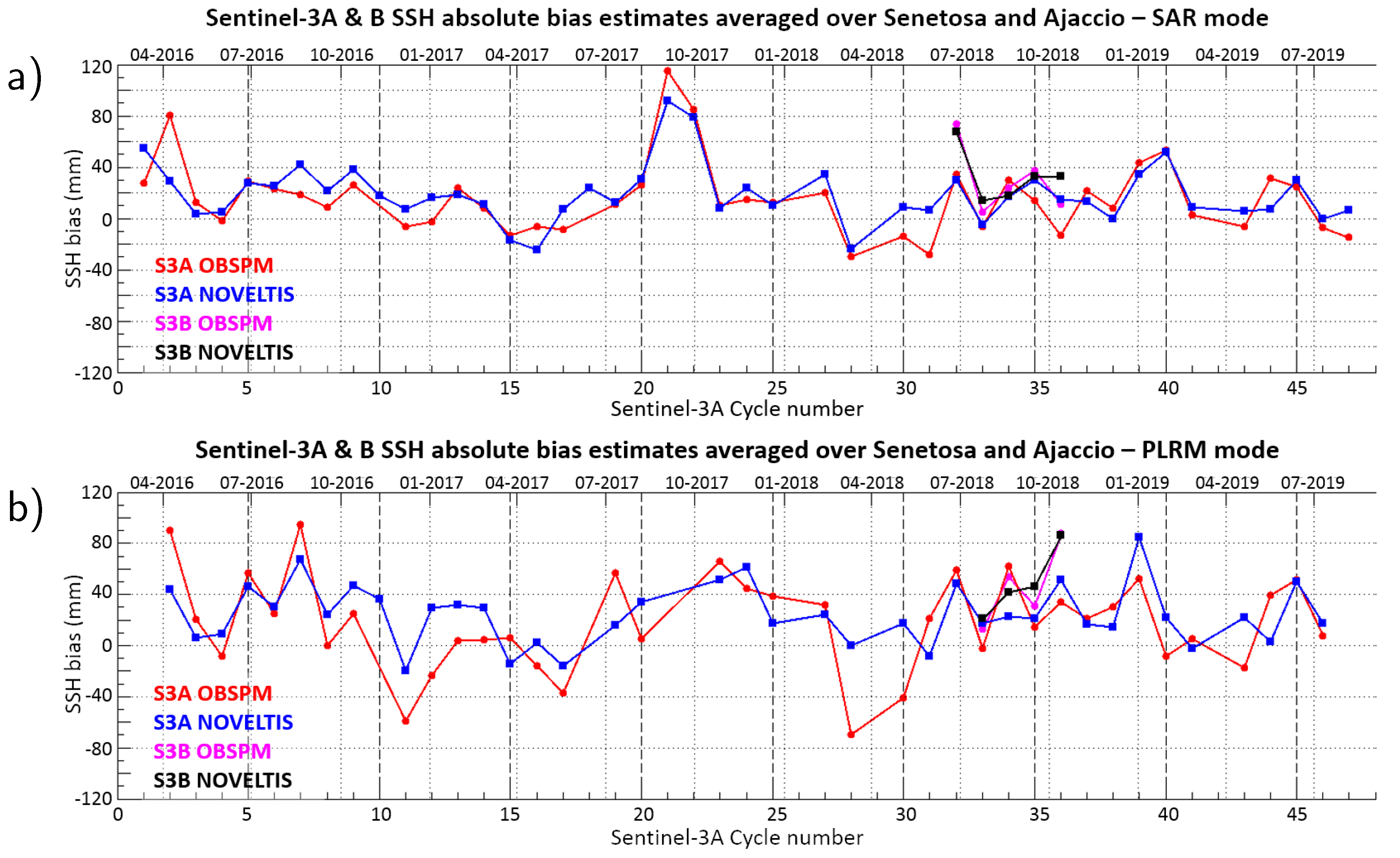
Figure 25.
Sentinel-3A and Sentinel-3B absolute SSH bias estimates on track 741, averaged over the Senetosa and Ajaccio sites for (a) SAR mode and (b) PLRM data, obtained with the two processing methods (OBSPM and NOVELTIS).
Figure 25.
Sentinel-3A and Sentinel-3B absolute SSH bias estimates on track 741, averaged over the Senetosa and Ajaccio sites for (a) SAR mode and (b) PLRM data, obtained with the two processing methods (OBSPM and NOVELTIS).
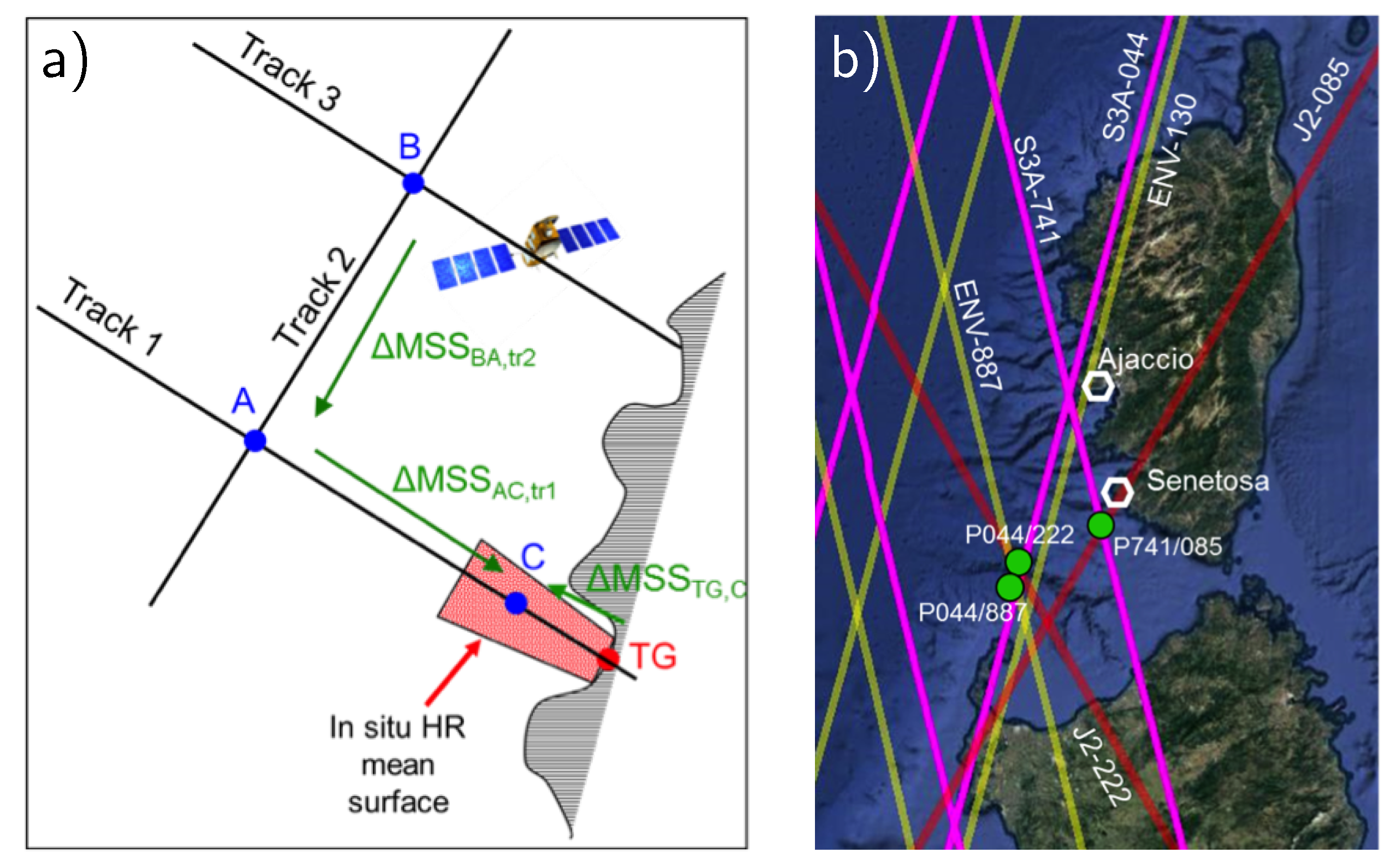
Figure 26.
(
a) Generic diagram of the regional calibration method (image taken from [
42]). (
b) Configuration in Corsica for the Sentinel-3A mission. S3A ground tracks in pink, Jason-2 tracks in red and Envisat tracks in yellow. The green dots show the crossover points where the offshore S3A SSH bias was computed in Senetosa.
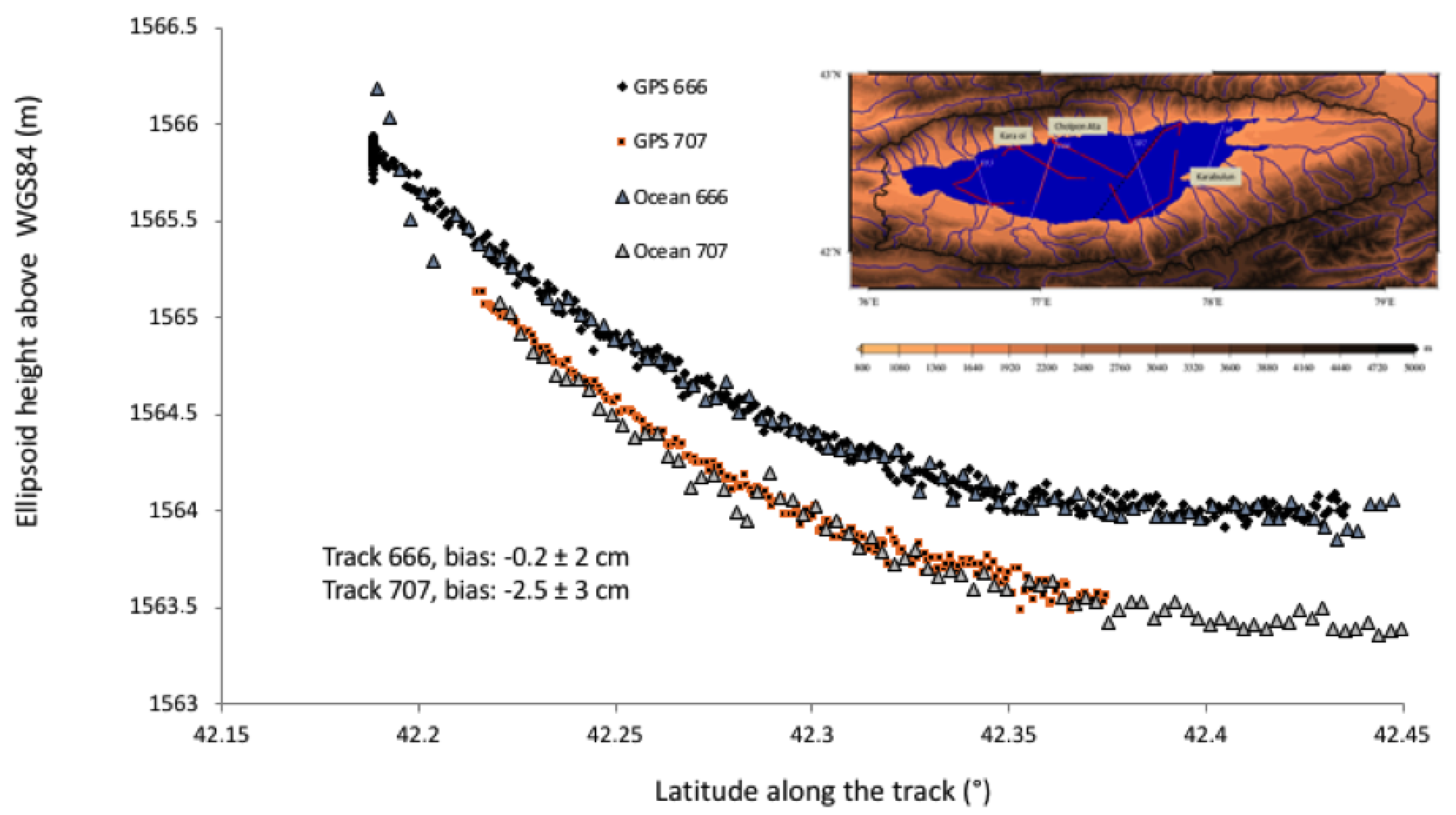
Figure 27.
Height of the lake surface above the reference ellipsoid as measured by Sentinel-3A with the Ocean retracker for cycle 9 (Oct. 2016), for the two tracks (666 and 707) and with the GNSS on the boat. (Inset shows the position of the tracks over the lake and the challenges of the high surrounding topography).
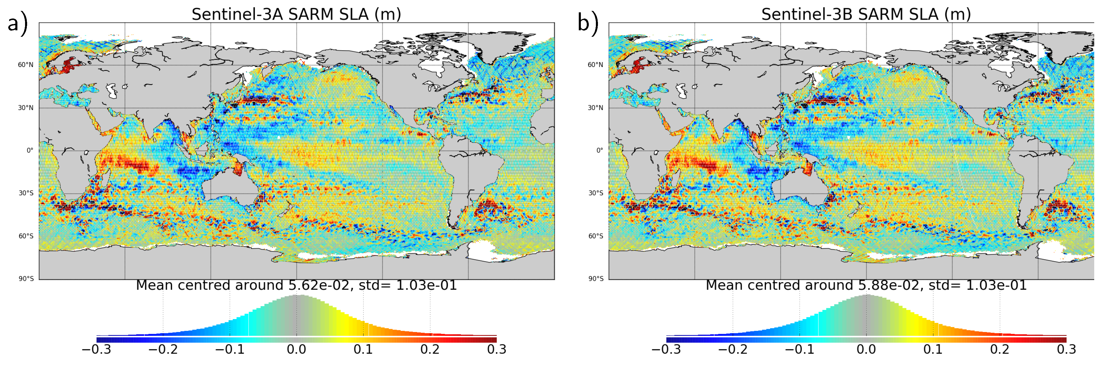
Figure 28.
Maps of Ku-band Sea Level Anomaly computed using radiometer Wet Tropospheric Correction over Sentinel-3B cycle 35 (i.e., from 25/01/2020 to 21/02/2020), for Sentinel-3A (a) and Sentinel-3B (b).
Figure 28.
Maps of Ku-band Sea Level Anomaly computed using radiometer Wet Tropospheric Correction over Sentinel-3B cycle 35 (i.e., from 25/01/2020 to 21/02/2020), for Sentinel-3A (a) and Sentinel-3B (b).
Figure 29.
Map of mean Sea Surface Height difference at Sentinel-3A SARM/Jason-3 crossovers, computed from April 2016 to September 2019, using Sentinel-3A 2020 reprocessed dataset. The mean bias of 1.97 cm has been removed before plotting.
Figure 29.
Map of mean Sea Surface Height difference at Sentinel-3A SARM/Jason-3 crossovers, computed from April 2016 to September 2019, using Sentinel-3A 2020 reprocessed dataset. The mean bias of 1.97 cm has been removed before plotting.
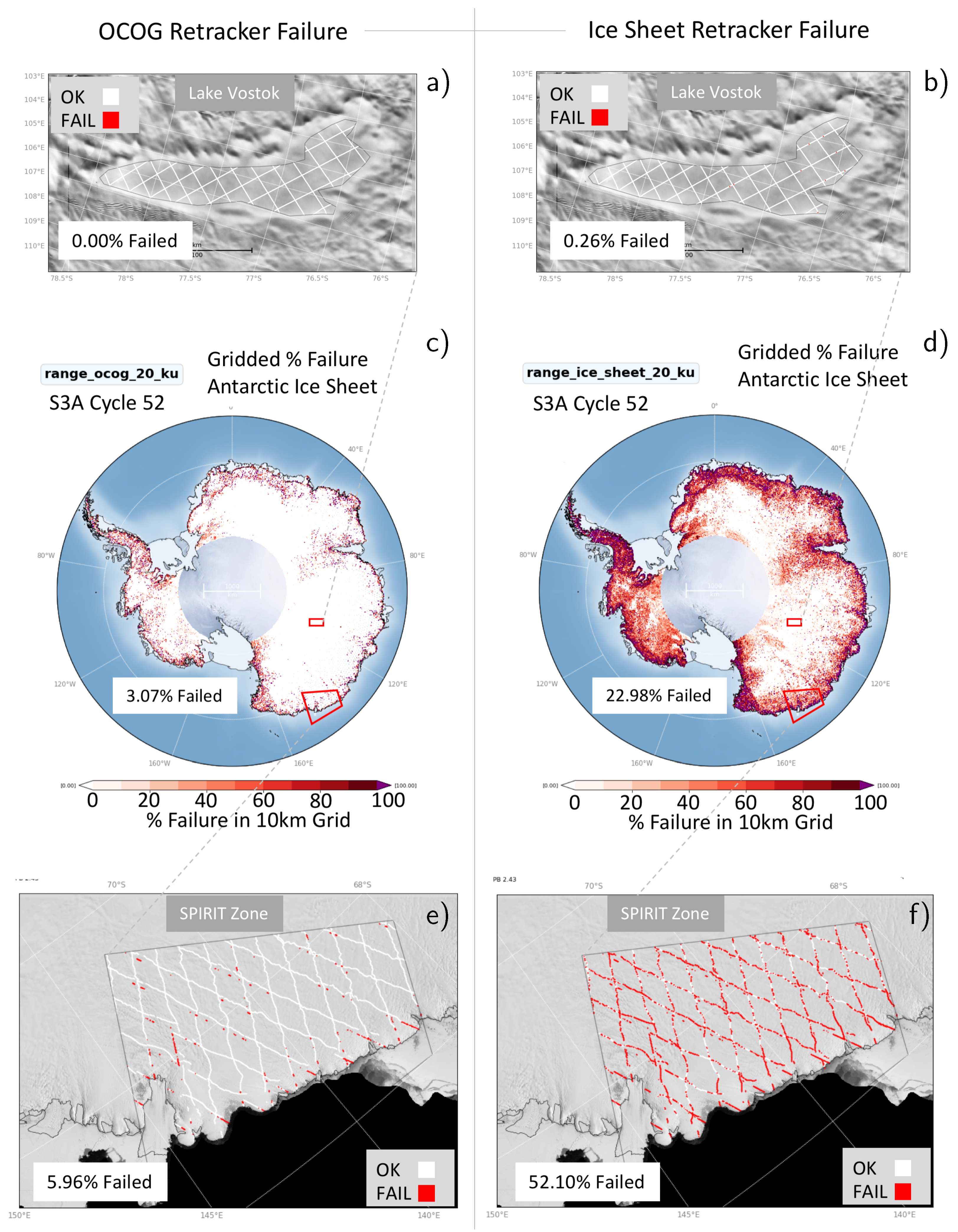
Figure 30.
Monitoring retracker failure for S3A Cycle 52 (PB2.43) over 3 different areas. (a,b) along-track failure over Lake Vostok area of low slope, (c,d) 10 km gridded percentage failure over the Antarctic ice sheet, (e,f) along-track failure over the SPIRIT marginal zone of high slope.
Figure 30.
Monitoring retracker failure for S3A Cycle 52 (PB2.43) over 3 different areas. (a,b) along-track failure over Lake Vostok area of low slope, (c,d) 10 km gridded percentage failure over the Antarctic ice sheet, (e,f) along-track failure over the SPIRIT marginal zone of high slope.
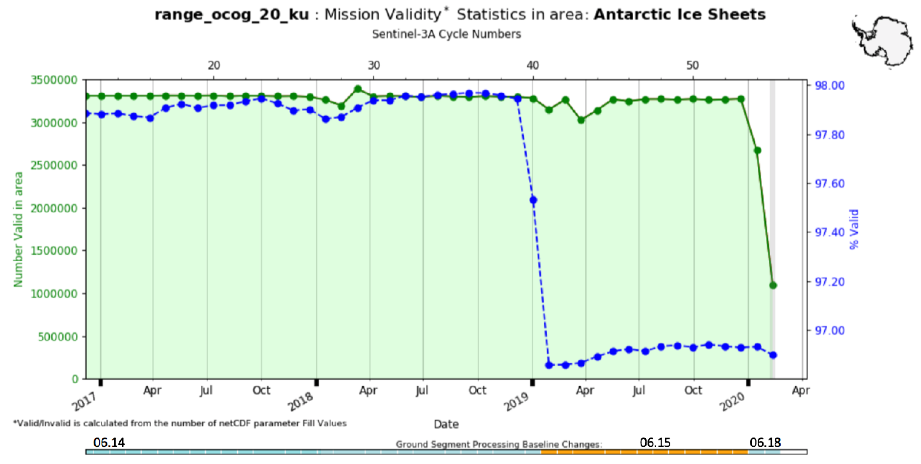
Figure 31.
Time series of retracker failure for S3A over the Antarctic ice sheets. The coloured line at the bottom indicates changes in processing baseline from PB2.31 until cycle 40, then PB2.43 and finally PB2.61. Note a decrease in % valid does not mean a reduction in performance, but rather better recognition of problem data.
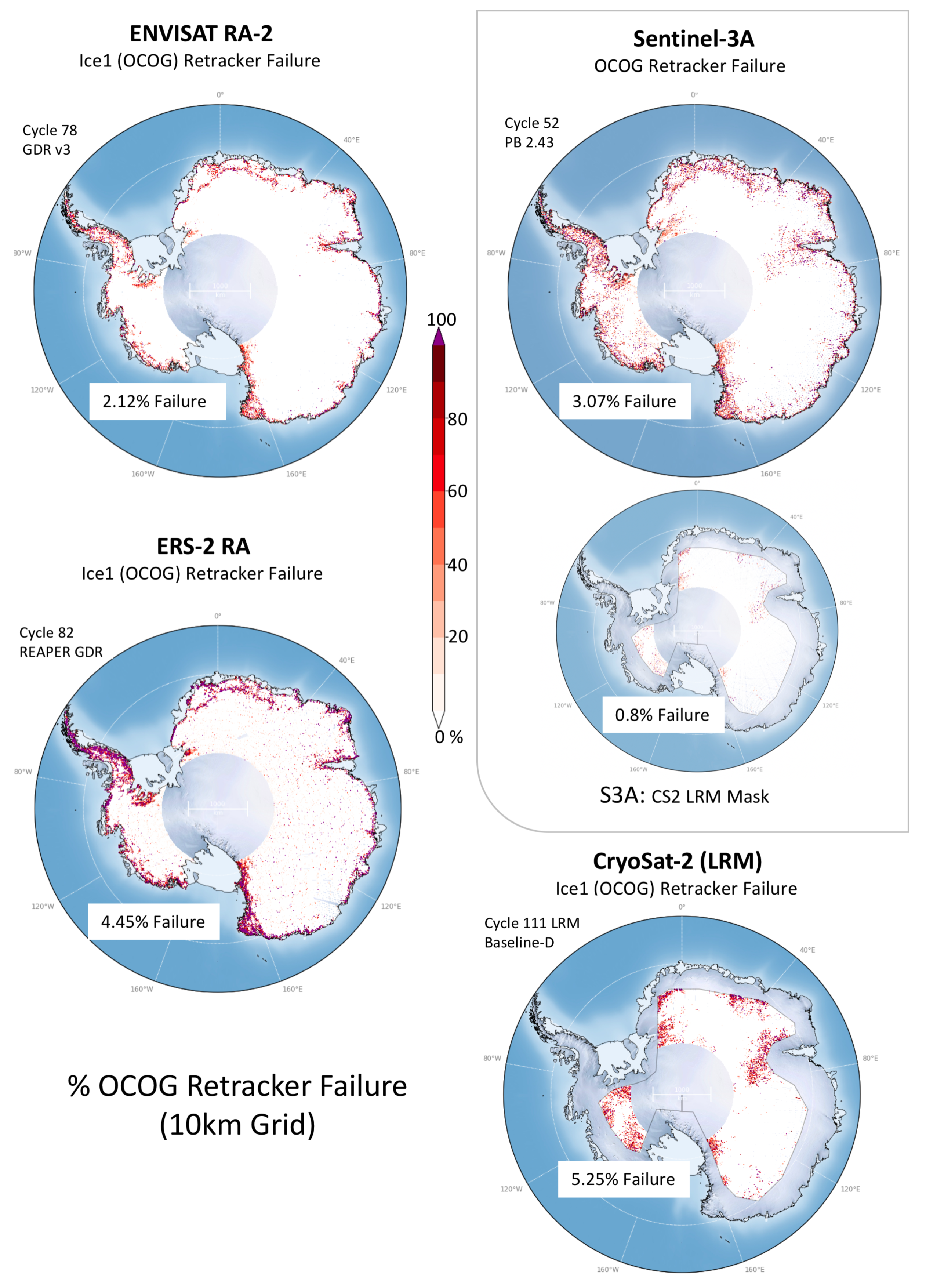
Figure 32.
Comparison of gridded percentage failure rates for OCOG retracker for S3A SAR, Envisat, ERS-2 and CryoSat-2 (LRM mode) over Antarctica.
Figure 32.
Comparison of gridded percentage failure rates for OCOG retracker for S3A SAR, Envisat, ERS-2 and CryoSat-2 (LRM mode) over Antarctica.
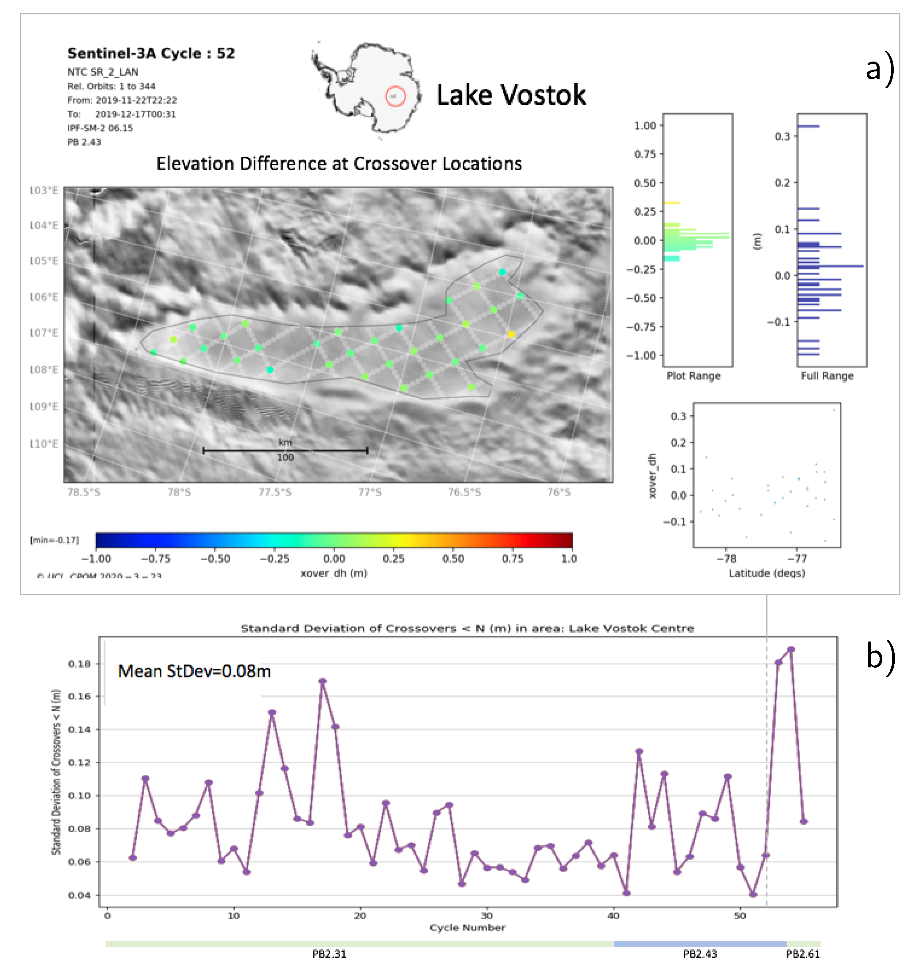
Figure 33.
OCOG elevation differences at single cycle orbit crossover locations over sub-glacial Lake Vostok. (a) Single cycle example (from Cycle 052), (b) S3A mission time series of standard deviation of differences, with dashed line showing how the selected cycle fits in.
Figure 33.
OCOG elevation differences at single cycle orbit crossover locations over sub-glacial Lake Vostok. (a) Single cycle example (from Cycle 052), (b) S3A mission time series of standard deviation of differences, with dashed line showing how the selected cycle fits in.
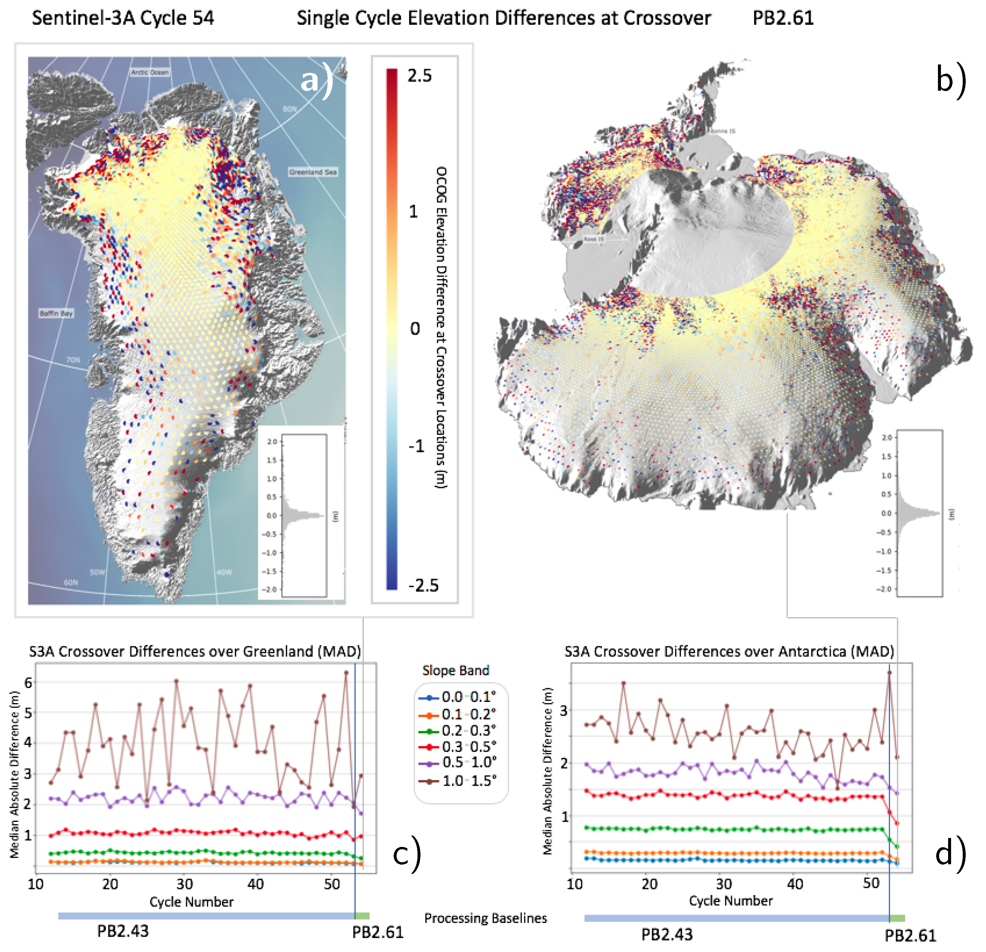
Figure 34.
OCOG elevation differences at single cycle orbit crossover locations over the (a) Greenland and (b) Antarctic ice sheets, and (c,d) mission time series of the Median Absolute Difference (MAD) of crossover differences per band of surface slope. The vertical lines highlight the impact of the change in PB.
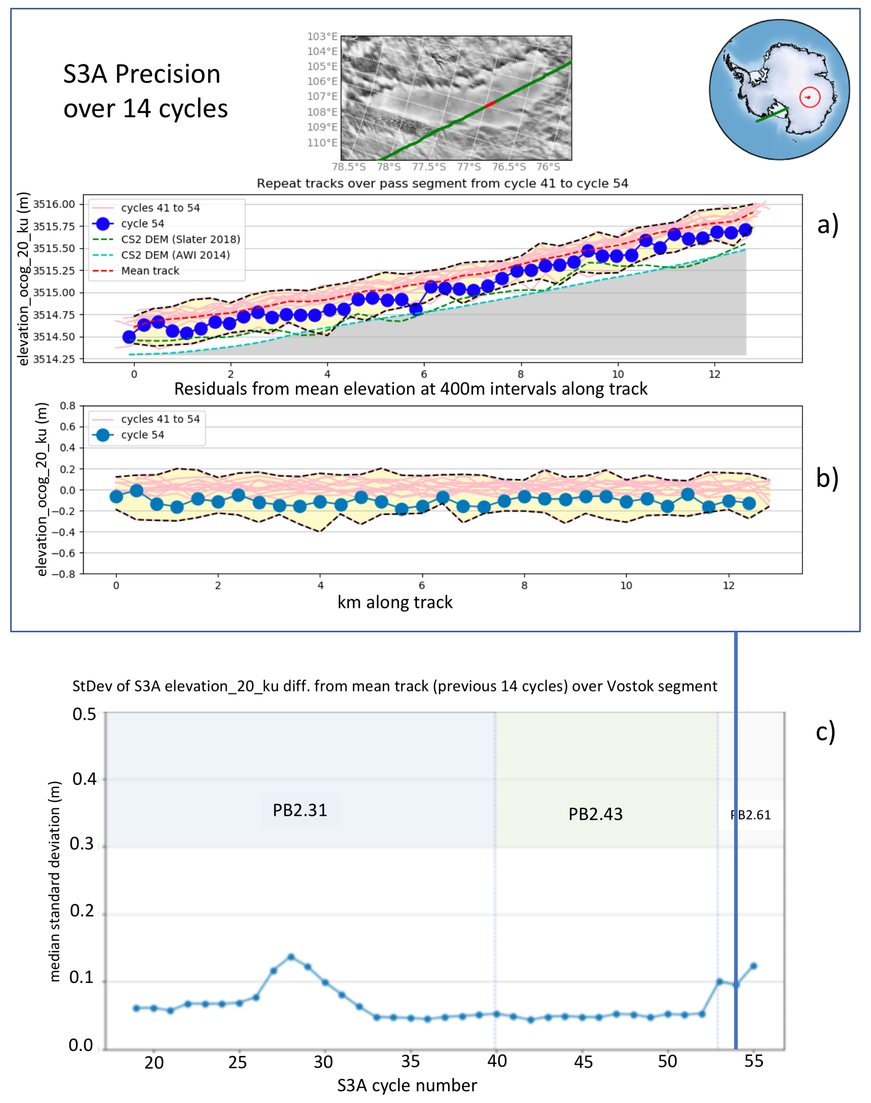
Figure 35.
Precision monitored using repeat tracks over Lake Vostok. (a) 14 successive elevation profiles along track. (b) Residuals of selected cycle relative to mean over preceding cycles (c) Variability of residuals as a function of cycle number.
Figure 35.
Precision monitored using repeat tracks over Lake Vostok. (a) 14 successive elevation profiles along track. (b) Residuals of selected cycle relative to mean over preceding cycles (c) Variability of residuals as a function of cycle number.
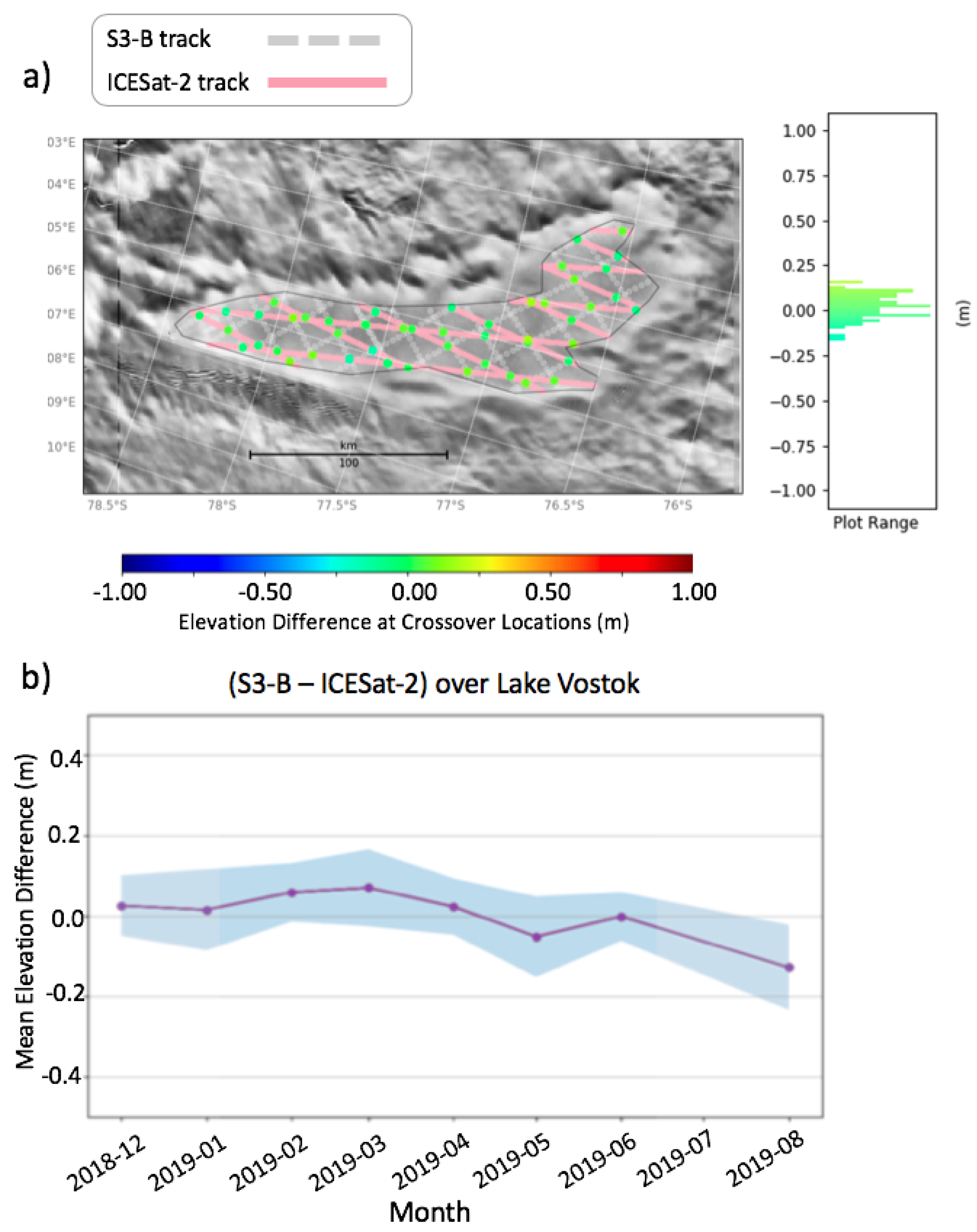
Figure 36.
Comparison of S3B with ICESat-2 over Lake Vostok for (a) April 2019 and (b) the mean monthly difference between December 2018 and August 2019.
Figure 36.
Comparison of S3B with ICESat-2 over Lake Vostok for (a) April 2019 and (b) the mean monthly difference between December 2018 and August 2019.
Figure 37.
Comparison of S3B with ICESat-2 over Antarctica and Greenland. (a) Map of crossover differences for April 2019. (b) Mean monthly difference between November 2018 and May 2019, with coloured lines representing different editing criteria.
Figure 37.
Comparison of S3B with ICESat-2 over Antarctica and Greenland. (a) Map of crossover differences for April 2019. (b) Mean monthly difference between November 2018 and May 2019, with coloured lines representing different editing criteria.
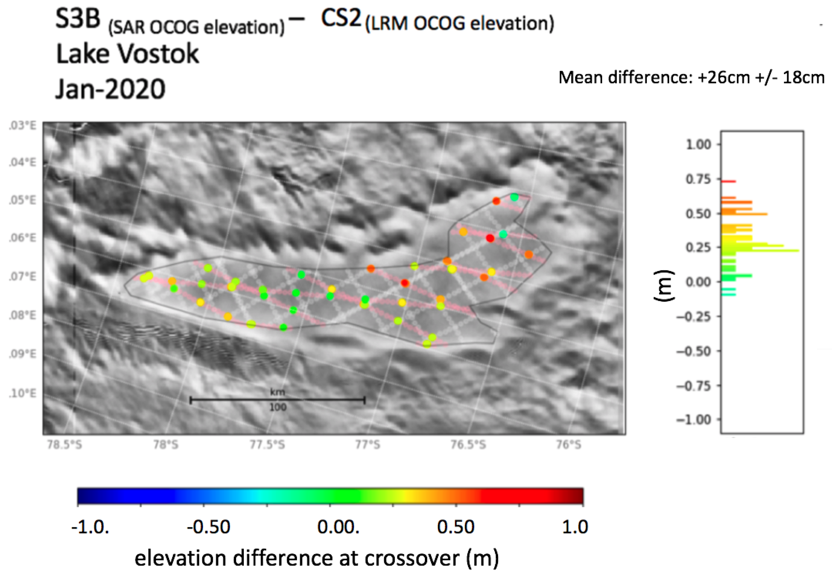
Figure 38.
Comparison of S3B with CryoSat-2 (LRM mode) over Lake Vostok. The plotted variable is the difference in heights recorded by S3B and CryoSat-2 at their mutual crossover points.
Figure 38.
Comparison of S3B with CryoSat-2 (LRM mode) over Lake Vostok. The plotted variable is the difference in heights recorded by S3B and CryoSat-2 at their mutual crossover points.
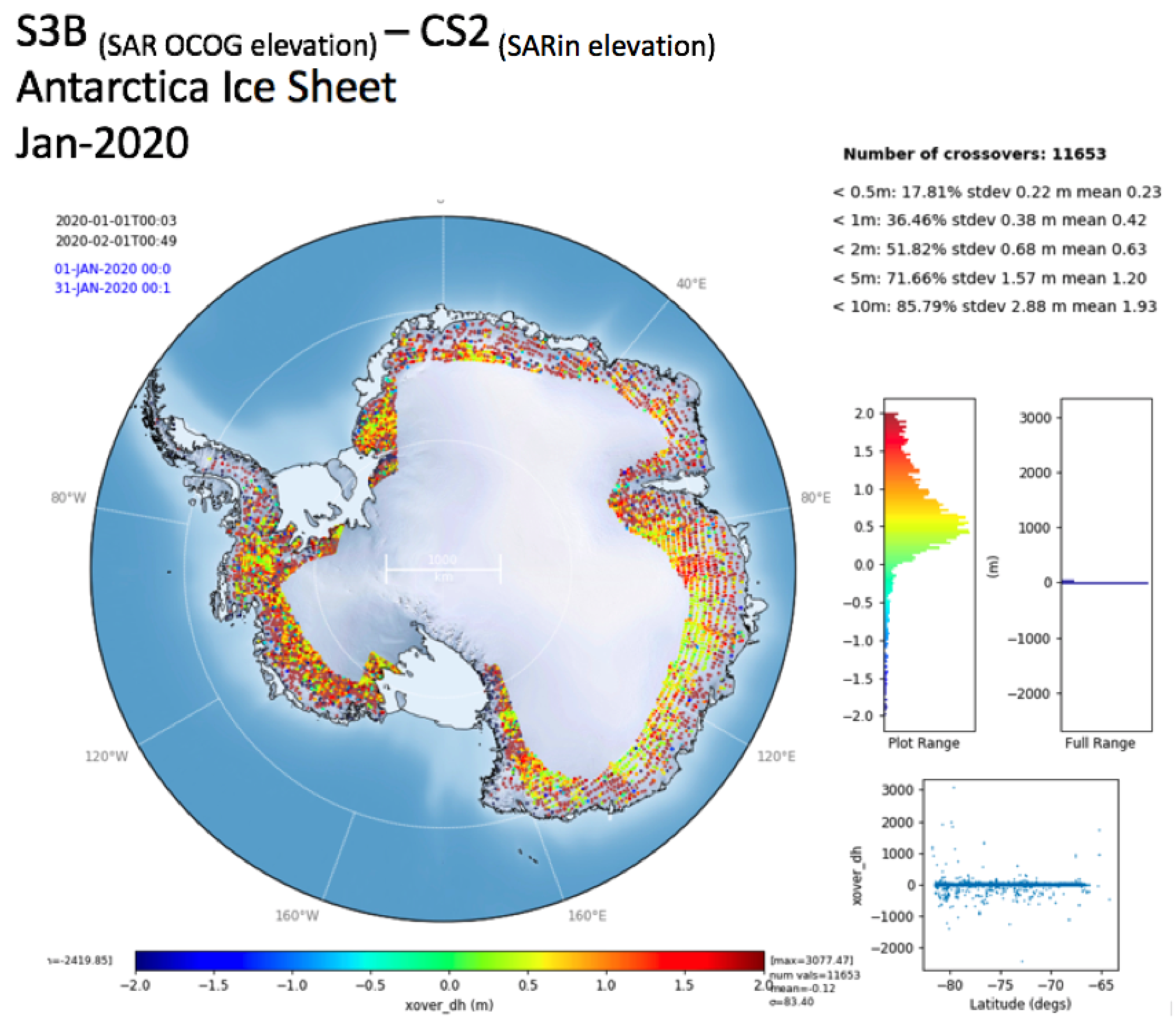
Figure 39.
Comparison of S3B with CryoSat-2 (SARin mode) over Antarctic margins.
Figure 39.
Comparison of S3B with CryoSat-2 (SARin mode) over Antarctic margins.
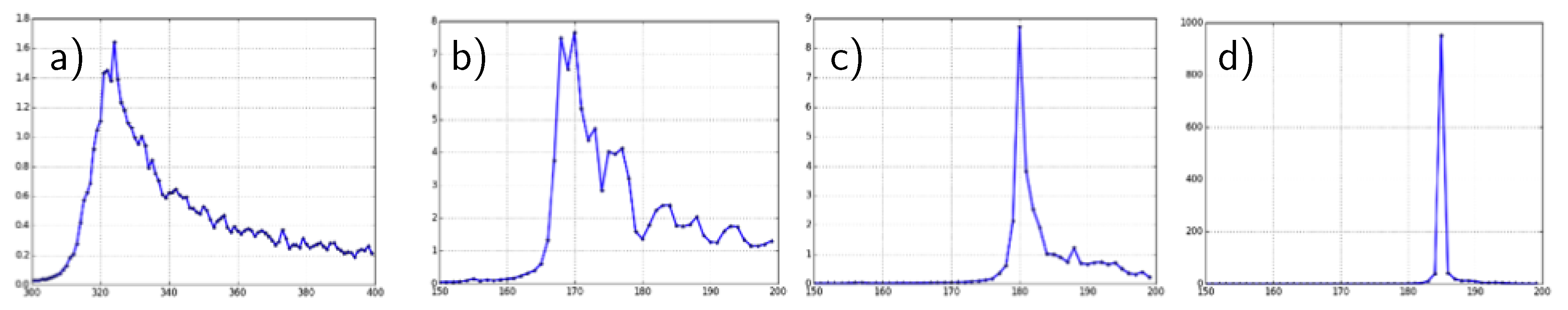
Figure 40.
Examples of SAR mode waveforms for 4 surface types: (a) open ocean, (b) thick pack ice, (c) thin pack ice and (d) ripple-free water within a lead in the ice. The waveforms differ both in shape and in backscattered power, which in these examples range by a factor of 1000.
Figure 40.
Examples of SAR mode waveforms for 4 surface types: (a) open ocean, (b) thick pack ice, (c) thin pack ice and (d) ripple-free water within a lead in the ice. The waveforms differ both in shape and in backscattered power, which in these examples range by a factor of 1000.
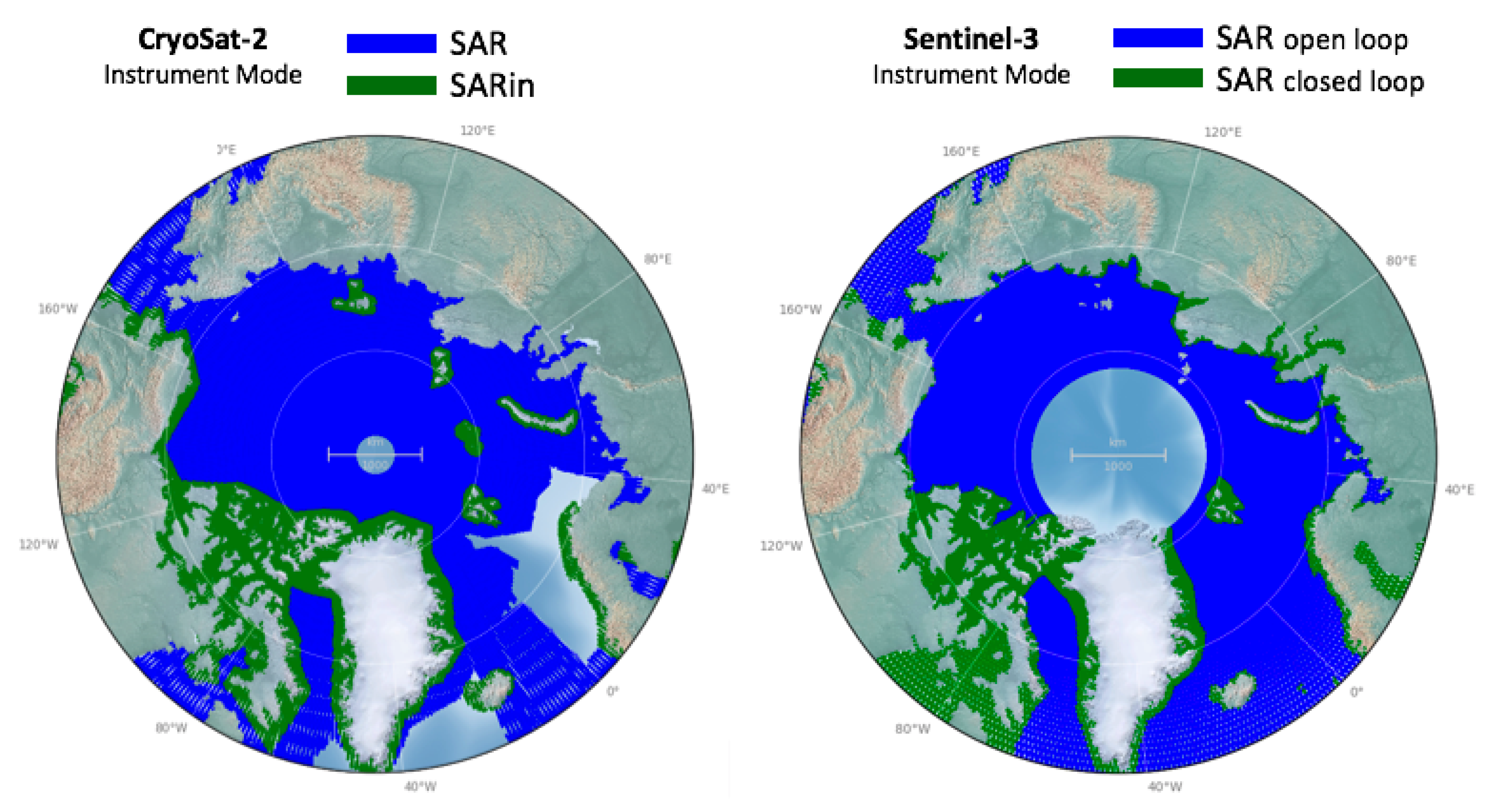
Figure 41.
Instrument modes used by CryoSat-2 and S3 over the Arctic. CryoSat-2 has a smaller polar hole (region of no observations) than S3, and CryoSat-2 operated in LRM mode over the ice-free regions along the coast of Norway and around the southern cape of Greenland.
Figure 41.
Instrument modes used by CryoSat-2 and S3 over the Arctic. CryoSat-2 has a smaller polar hole (region of no observations) than S3, and CryoSat-2 operated in LRM mode over the ice-free regions along the coast of Norway and around the southern cape of Greenland.
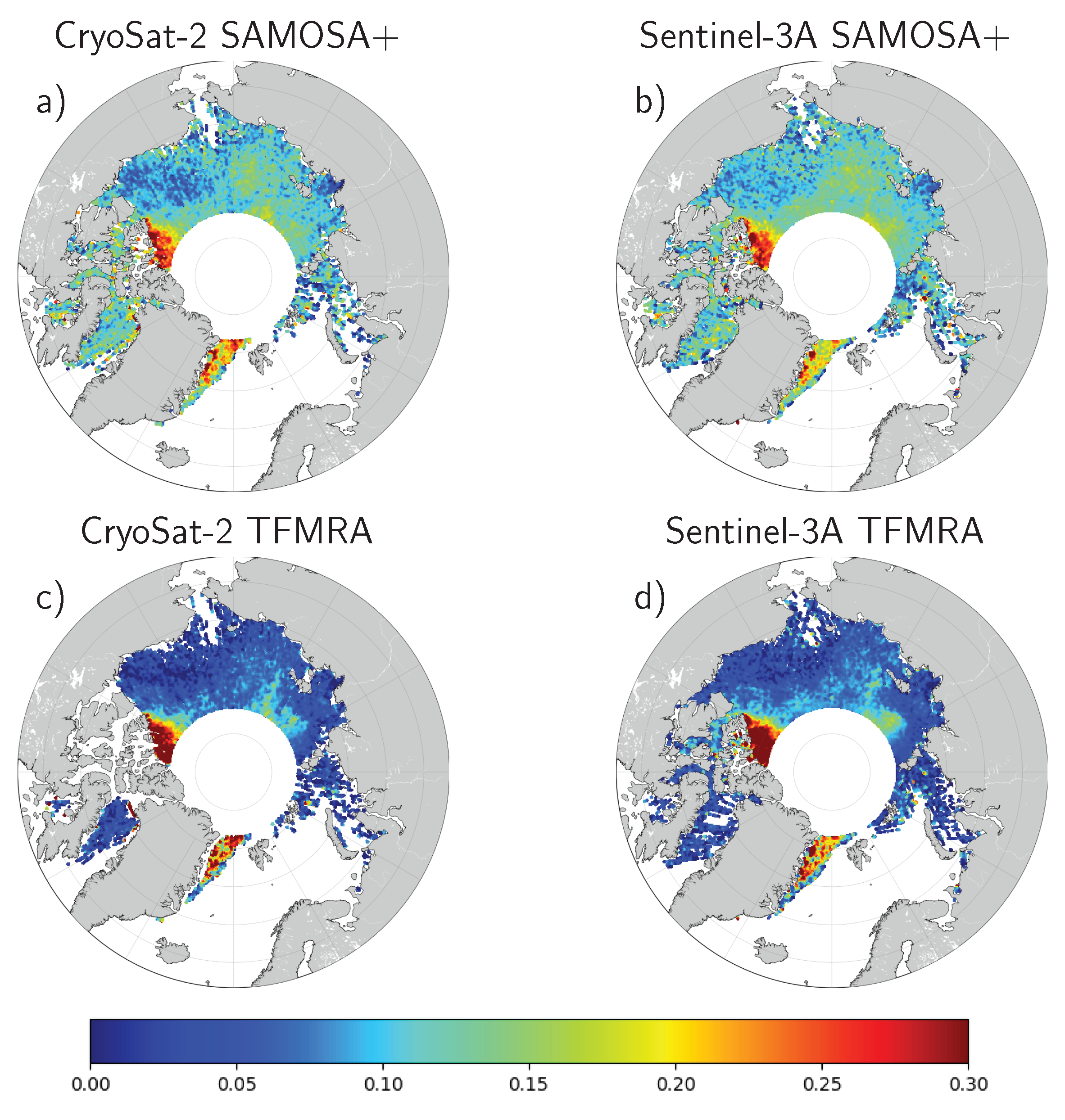
Figure 42.
Comparison of sea ice freeboard measurements for December 2016. CryoSat-2 (a,c) and Sentienl-3A (b,d), and with SAMOSA+ retracker (a,b) and TFMRA50 (c,d).
Figure 42.
Comparison of sea ice freeboard measurements for December 2016. CryoSat-2 (a,c) and Sentienl-3A (b,d), and with SAMOSA+ retracker (a,b) and TFMRA50 (c,d).
Figure 43.
Scatter distribution of in situ water height from the historical gauges and the Sentinel-3A measurements. The RMS of the differences is 1.5 cm.
Figure 43.
Scatter distribution of in situ water height from the historical gauges and the Sentinel-3A measurements. The RMS of the differences is 1.5 cm.
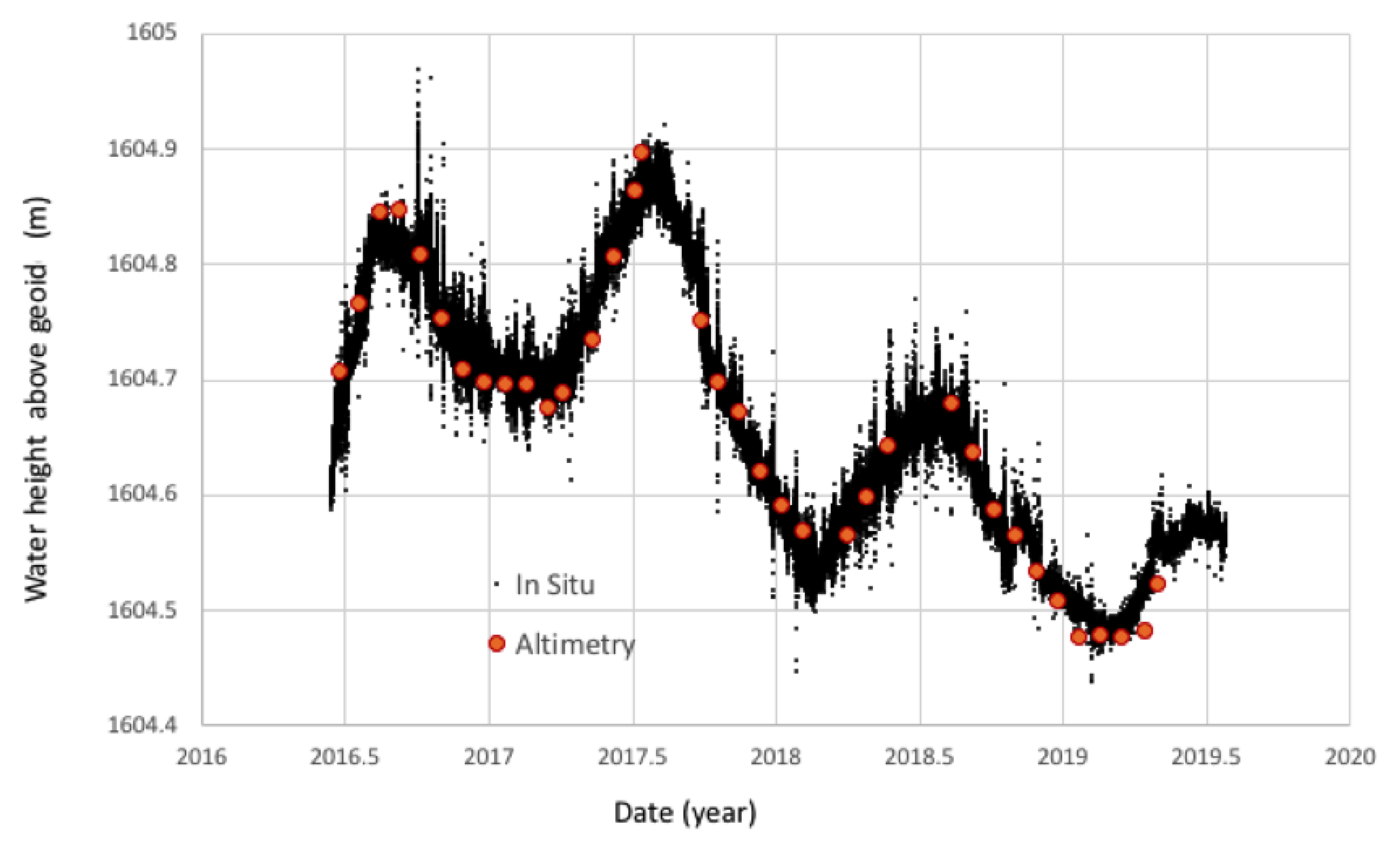
Figure 44.
Water height time series using the limnigraph in Karabulun and Sentinel-3A.
Figure 44.
Water height time series using the limnigraph in Karabulun and Sentinel-3A.
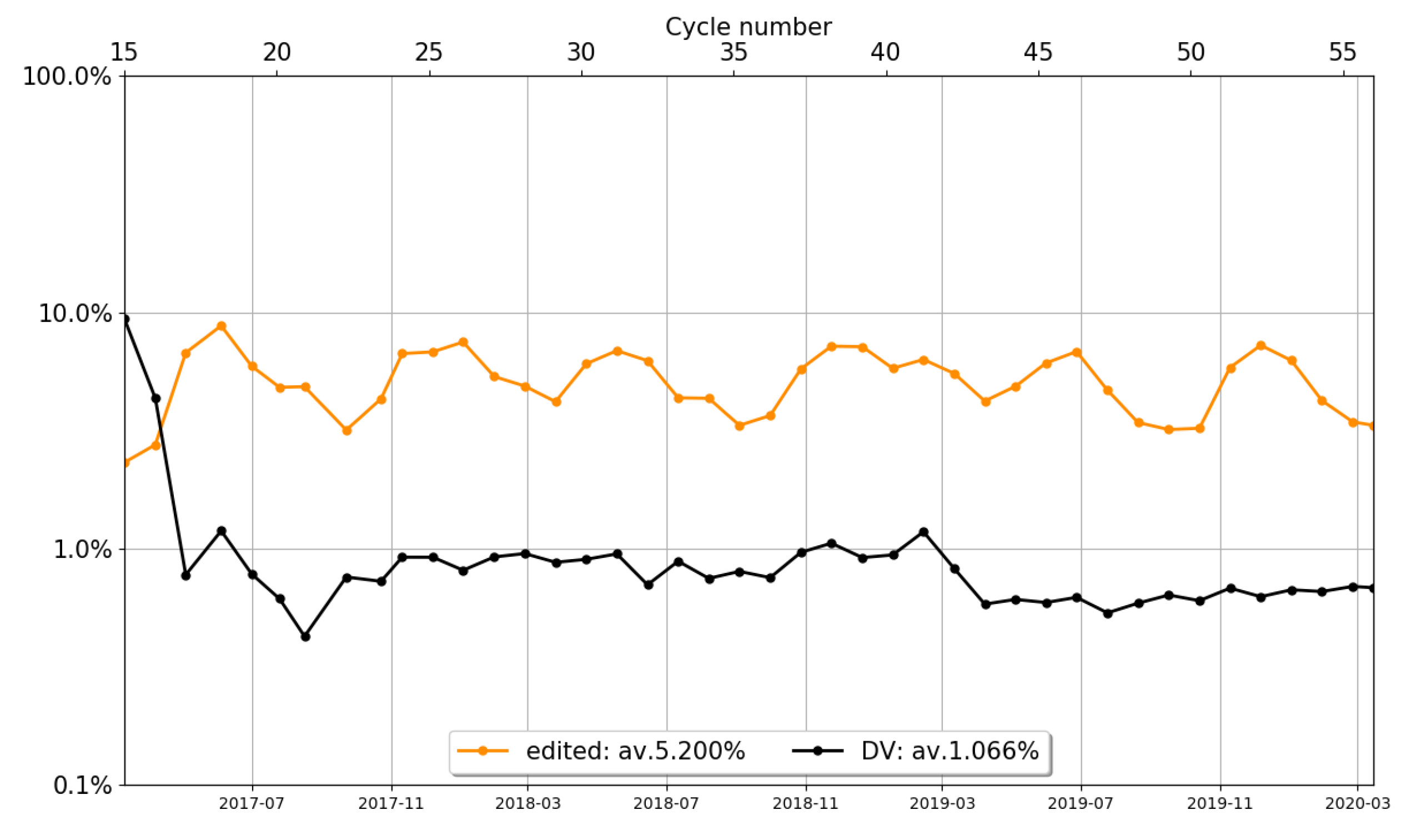
Figure 45.
Percentage of default values and edited measurements over lakes for the OCOG backscatter coefficient for Sentinel-3A.
Figure 45.
Percentage of default values and edited measurements over lakes for the OCOG backscatter coefficient for Sentinel-3A.
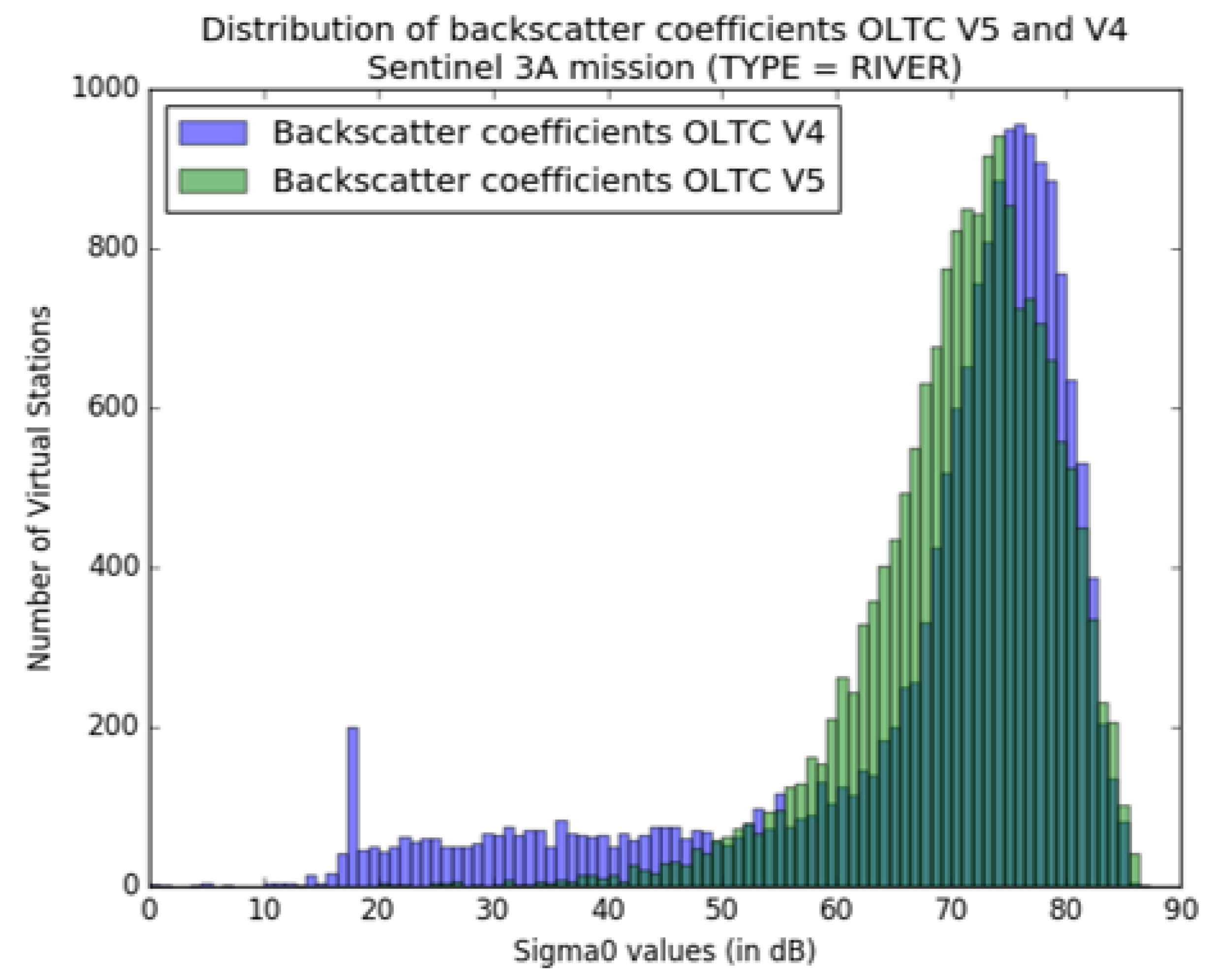
Figure 46.
Distribution of values for S3A with OLTC v4.2 (blue) and v5.0 (green) over approximately 17000 river targets.
Figure 46.
Distribution of values for S3A with OLTC v4.2 (blue) and v5.0 (green) over approximately 17000 river targets.
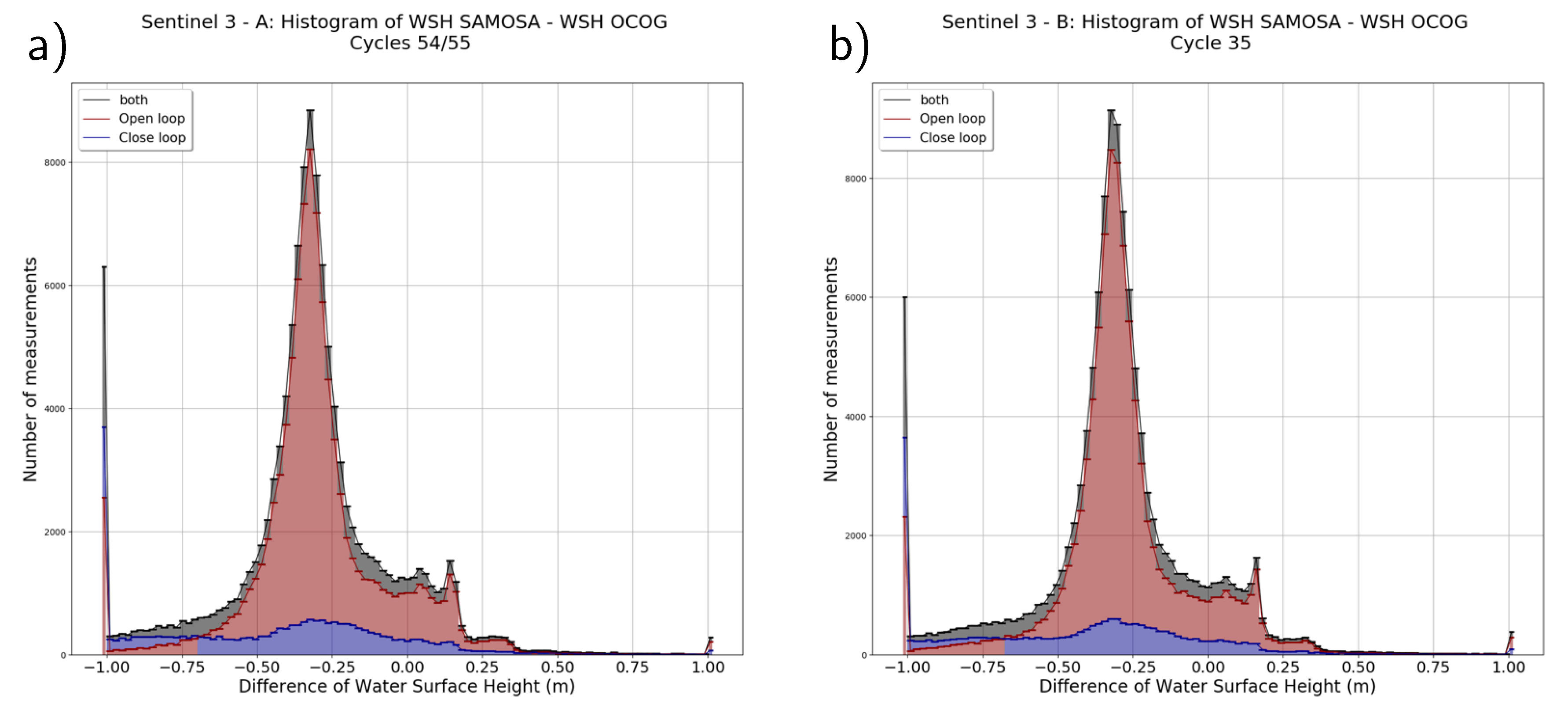
Figure 47.
Difference of Water Surface Height estimates between SAMOSA retracker and OCOG retracker for (a) Sentinel-3A and (b) Sentinel-3B, both for the 27-day period of Sentinel-3B cycle 35.
Figure 47.
Difference of Water Surface Height estimates between SAMOSA retracker and OCOG retracker for (a) Sentinel-3A and (b) Sentinel-3B, both for the 27-day period of Sentinel-3B cycle 35.
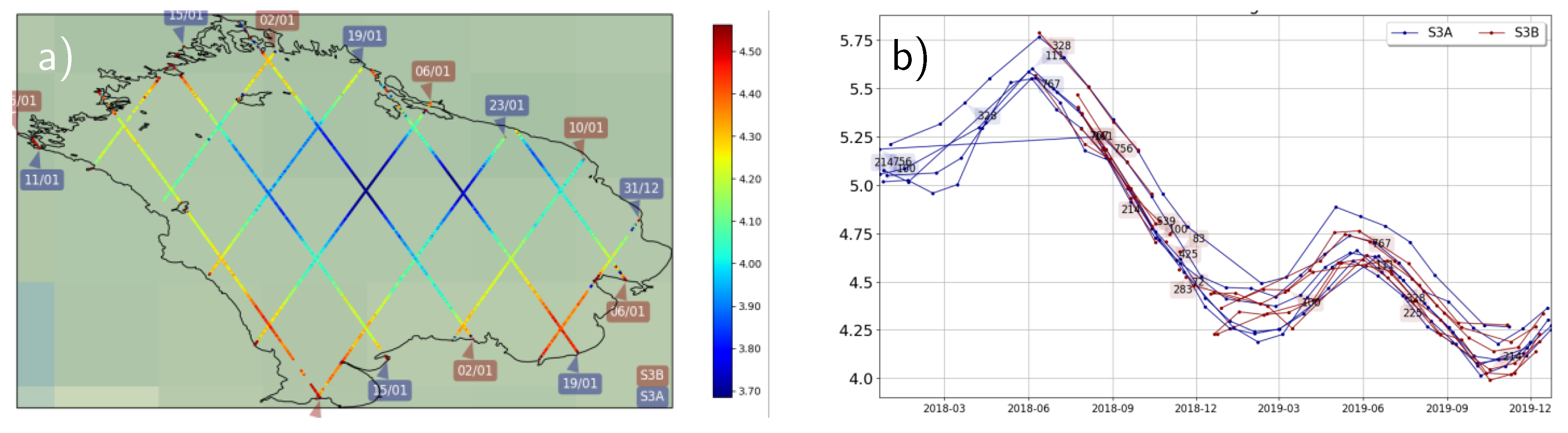
Figure 48.
Monitoring of water levels in Lake Ladoga (a) Map showing WSH (m) measured along different S3A and S3B tracks (b) Time series for each track, specified by pass number (S3A in blue, S3B in red. During its tandem mission (Jul.–Oct. 2018) S3B flew the same tracks as S3A; after Nov. 23th 2018 S3B was in it final interleaved orbit.
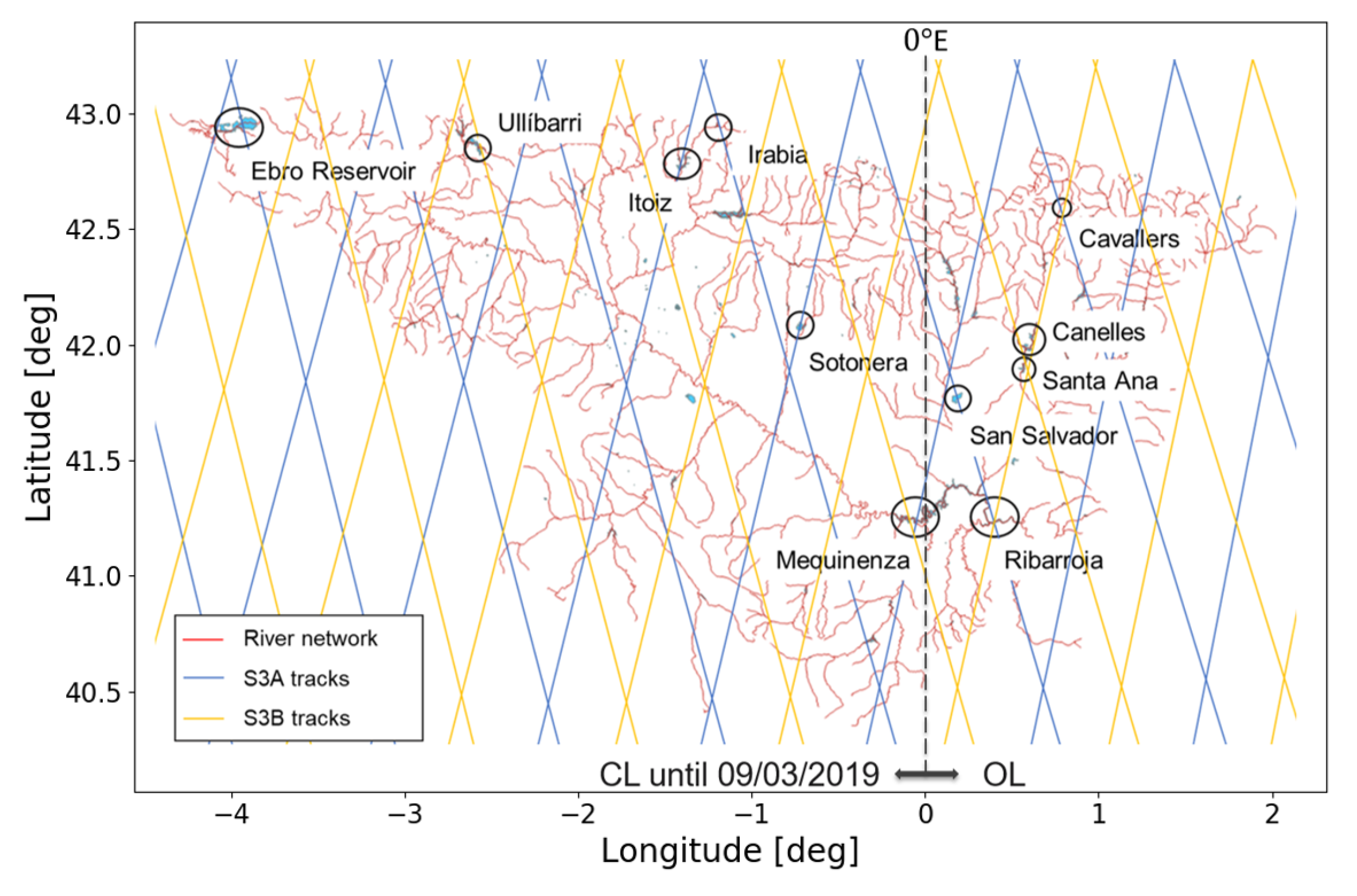
Figure 49.
Map of Ebro basin showing key rivers and reservoirs.
Figure 49.
Map of Ebro basin showing key rivers and reservoirs.
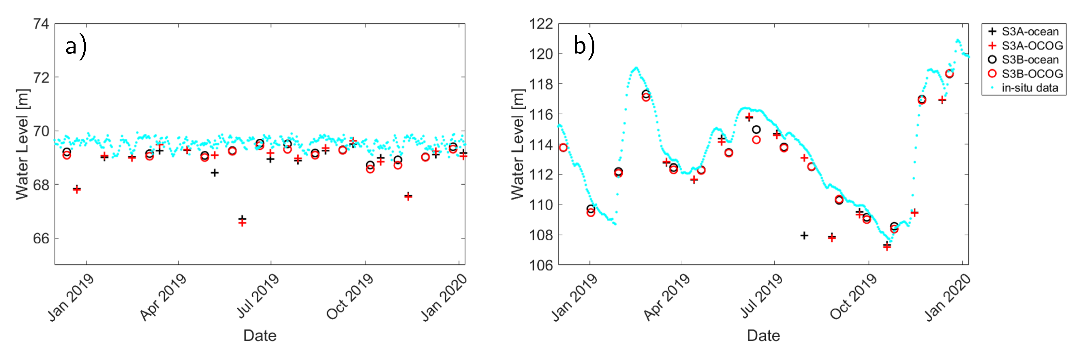
Figure 50.
Time series of S3A and S3B L2 derived water level over (a) Ribarroja Reservoir, (b) Mequinenza Reservoir.
Figure 50.
Time series of S3A and S3B L2 derived water level over (a) Ribarroja Reservoir, (b) Mequinenza Reservoir.
Table 1.
Levels and latencies of Sentinel-3 STM processing. The NRT data are provided in segments as downloaded from the satellite; data for the other latencies are collated in pole-to-pole passes (half orbits).
Table 1.
Levels and latencies of Sentinel-3 STM processing. The NRT data are provided in segments as downloaded from the satellite; data for the other latencies are collated in pole-to-pole passes (half orbits).
| Level |
|---|
| Level 0 | Raw telemetered data |
| Level 1A | Geolocated and fully calibrated |
| Level 1BS | L1A + fully beamformed → “stack” |
| Level 1B | Multi-look processed → SAR waveforms |
| Level 2 | Retracked → Geophysical estimates + corrections |
| Latency |
| Near Real-Time (NRT) | Within 3 h |
| Short Time Critical (STC) | Within 48 h |
| Non-Time Critical (NTC) | Within 1 month |
| Full Mission reprocessing (FMR) | When needed |
Table 2.
Results over transponders.
Table 2.
Results over transponders.
| TRP Position | Crete | | Svalbard |
|---|
| | S3A (46 Passes) | S3B (18 Passes) | | S3A (9 Passes) | S3B (10 Passes) |
|---|
| Range Bias [mm] | 6.79 | −6.59 | | −109.92 | −68.44 |
| Datation Bias [microseconds] | −125.95 | −25.47 | | −84.94 | −43.29 |
| Range Stack Alignment [mm/beam] | 0.07 | 0.02 | | 0.07 | 0.02 |
| Range Noise [mm] | 0.81 | 0.83 | | 15.30 | 6.93 |
Table 3.
Statistics on the Sentinel-3A and Sentinel-3B SAR and PLRM absolute SSH bias estimates in Corsica (track 741).
Table 3.
Statistics on the Sentinel-3A and Sentinel-3B SAR and PLRM absolute SSH bias estimates in Corsica (track 741).
| Satellite | Processing Centre | SAR | | PLRM |
|---|
| | | SSH Bias (mm) | # Cycles | | SSH Bias (mm) | # Cycles |
|---|
| Senetosa |
| S3A | OBSPM | | 47 | | | 46 |
| S3A | NOVELTIS | | 47 | | | 46 |
| S3B | OBSPM | | 4 | | | 4 |
| S3B | NOVELTIS | | 4 | | | 4 |
| Ajaccio |
| S3A | OBSPM | | 42 | | | 38 |
| S3A | NOVELTIS | | 44 | | | 40 |
| S3B | OBSPM | | 4 | | | 4 |
| S3B | NOVELTIS | | 4 | | | 4 |
| Mean |
| S3A | OBSPM | | 42 | | | 38 |
| S3A | NOVELTIS | | 44 | | | 39 |
| S3B | OBSPM | | 4 | | | 4 |
| S3B | NOVELTIS | | 4 | | | 4 |
Table 4.
Statistics on the Sentinel-3A SAR and PLRM SSH absolute regional SSH bias estimates off Senetosa.
Table 4.
Statistics on the Sentinel-3A SAR and PLRM SSH absolute regional SSH bias estimates off Senetosa.
| Senetosa | SAR | | PLRM |
|---|
| PB 2.33 (S3MPC) | Mean | STD | # Cycles | | Mean | STD | # Cycles |
|---|
| Cycles1-26 | (mm) | (mm) | | | (mm) | (mm) | |
|---|
| Track 741 (local) | | 24 | 24 | | | 28 | 23 |
| no ocean dyn. corr. | | | | | | | |
| Track 741 (local) | | 26 | 24 | | | 30 | 23 |
| Track 741 X J2 085 | | 31 | 24 | | | 36 | 23 |
| Track 044 X Env 887 | | 33 | 25 | | | 47 | 23 |
| Track 044 X J2 222 | | 27 | 25 | | | 40 | 23 |
| Regional mean | | 29 | 25 | | | 38 | 23 |
Table 5.
Results of the water level comparison with in situ data over the S3A long term monitored reservoirs (June 2016–December 2019).
Table 5.
Results of the water level comparison with in situ data over the S3A long term monitored reservoirs (June 2016–December 2019).
| Reservoir | Width | Track | Tracking Mode | RMSE/Bias/MD [m] |
|---|
| | | | | L2 Ocean | L2 OCOG |
|---|
| Ebro | 1.8 km | S3A 014 | CL→ OL | 3.6/−1.0/1.91 | 2.2 /−0.76/1.32 |
| Sotonera | 4.5 km | S3A 222 | CL→ OL | 1.3/−0.96/0.96 | 1.15/−0.98 /0.98 |
| Ribarroja | 400 m | S3A 242 | OL | 0.77/−0.55/0.55 | 0.77/−0.52/ 0.52 |
| Cavallers | 800 m | S3A 299 | OL | Off-track |
| San Salvador | 800 m | S3A 299 | OL | Off-track |
Table 6.
Results of the S3B water level comparison with in situ data (December 2018–December 2019).
Table 6.
Results of the S3B water level comparison with in situ data (December 2018–December 2019).
| Reservoir | Width | Track | Tracking Mode | RMSE/Bias/MD [m] |
|---|
| | | | | L2 Ocean | L2 OCOG |
|---|
| Ullibarri | 260 m | S3B 128 | OL | 2.89/0.3/1.48 | 0.89/−0.89/0.89 |
| Canelles | 260 m | S3B 299 | OL | 1.96/−1.3/1.3 | 2.05/−1.4/1.4 |
| Santa Ana | 300 m–1.8 km | S3B 299 | OL | 0.89/−0.88/0.88 | 1.05/−1.04/1.04 |
Table 7.
Results of the S3A and S3B water level comparison with in situ data (December 2018–December 2019).
Table 7.
Results of the S3A and S3B water level comparison with in situ data (December 2018–December 2019).
| Reservoir | Width | Track | Tracking Mode | RMSE/Bias/MD [m] |
|---|
| | | | | L2 Ocean | L2 OCOG |
|---|
| Ribarroja | 400 m | S3A 242 | OL | 1.17/−0.88/0.89 | 1.15/−0.82/0.82 |
| | | S3B 336 | | 0.43/−0.38/0.39 | 0.52/−0.48/0.48 |
| Mequinenza | 600 m | S3A 279 | OL | 2.32/−1.6/1.6 | 1.58/−1.18/1.18 |
| | | S3B 242 | | 0.64/−0.49/0.59 | 0.78/−0.61/0.67 |

 ,
, 


