
Hyperspectral Dimensionality Reduction Based on Inter-Band Redundancy Analysis and Greedy Spectral Selection †


1
Gianforte School of Computing, Montana State University, Bozeman, MT 59717, USA
2
Department of Electrical and Computer Engineering, Montana State University, Bozeman, MT 59717, USA
3
Optical Technology Center, Montana State University, Bozeman, MT 59717, USA
*
Author to whom correspondence should be addressed.
†
This paper is an extended version of our paper published in International Joint Conference on Neural Networks (virtual event, 18–22 July 2021).
Remote Sens. 2021, 13(18), 3649; https://doi.org/10.3390/rs13183649
Submission received: 28 July 2021
/
Revised: 3 September 2021
/
Accepted: 9 September 2021
/
Published: 13 September 2021
(This article belongs to the Special Issue Innovative Application of AI in Remote Sensing)
Abstract
:Hyperspectral imaging systems are becoming widely used due to their increasing accessibility and their ability to provide detailed spectral responses based on hundreds of spectral bands. However, the resulting hyperspectral images (HSIs) come at the cost of increased storage requirements, increased computational time to process, and highly redundant data. Thus, dimensionality reduction techniques are necessary to decrease the number of spectral bands while retaining the most useful information. Our contribution is two-fold: First, we propose a filter-based method called interband redundancy analysis (IBRA) based on a collinearity analysis between a band and its neighbors. This analysis helps to remove redundant bands and dramatically reduces the search space. Second, we apply a wrapper-based approach called greedy spectral selection (GSS) to the results of IBRA to select bands based on their information entropy values and train a compact convolutional neural network to evaluate the performance of the current selection. We also propose a feature extraction framework that consists of two main steps: first, it reduces the total number of bands using IBRA; then, it can use any feature extraction method to obtain the desired number of feature channels. We present classification results obtained from our methods and compare them to other dimensionality reduction methods on three hyperspectral image datasets. Additionally, we used the original hyperspectral data cube to simulate the process of using actual filters in a multispectral imager.
1. Introduction
Optical remote sensing systems are predicated on analyzing the spatial and spectral information contained within the imagery they collect. Due to this ability, the applications of remote sensing are widespread, ranging from measurements for precision agriculture [1] to applications in forensic sciences [2]. In many of these applications, the spatial information carried in the image must be considered when classifying objects in a scene; however, the spectral information plays a crucial role in the process. The ability to maintain spatial detail while also generating several spectral channels has given rise to several different forms of passive remote sensing imaging systems, ranging from multispectral imaging (MSI) [3,4] to hyperspectral imaging systems (HSIs) [5,6]. As opposed to MSI systems, which capture several discrete spectral bands, HSI systems capture hundreds of contiguous spectral bands. The utility of each type of imaging system varies based on the goal of the work. For example, if spectral bands are known a priori, MSI systems are often advantageous as the specific spectral bands can be measured directly with a relatively simple system and data products. However, if the spectral bands for a certain application are unknown, HSI can become a powerful tool.
Hyperspectral imaging systems have the ability to capture good spatial resolution while also capturing rich spectral content. However, the spectrally dense data cubes captured by HSI systems often have large file sizes, high data density, and introduce additional computational complexity. Taken together, these factors present computational limitations when postprocessing imagery and storing data products. For example, the Hyperspectral Infrared Imager (HyspIRI) launched by the Jet Propulsion Laboratory (JPL) of the National Aeronautics and Space Administration (NASA) has an average continuous data rate of 65 Mb/s, which produces a daily data volume of 5.2 Tb [7]; therefore, the inherent computational cost makes fast onboard processing difficult.
In applications with smoothly varying spectral features, the additional complexity and cost introduced by HSI systems may be unnecessary. For example, plant stress is often estimated with the Normalized Difference Vegetation Index (NDVI) using a single red band and a single near-infrared band instead of an HSI system, as is the case for the Advanced Very High-Resolution Radiometer (AVHRR) instrument of the National Oceanic and Atmospheric Administration (NOAA) [8] or the drone-based MicaSense RedEdge-MX sensor [9]. Yet, for many applications, there is a need to resolve sharp spectral features or the salient wavelengths are not known a priori, meaning MSI systems would provide little value. Though HSI systems capture rich spectral data, the determination of the most relevant wavelengths in a data cube is a challenging task. The successful determination of salient wavelengths within a hyperspectral data cube would provide several distinct benefits. If using a band selection method, the processing and storage requirements can be relaxed as only relevant spectral bands are stored and processed [10]. When using feature extraction methods, all spectral bands are stored, but classification accuracy can be increased [11]. Regardless of which method is used, the identification of relevant spectral bands provides a means of developing multispectral imagers in place of hyperspectral imagers for a given classification task, with applications ranging from precision agriculture [12] to dermatology [13].
In this paper, we present a dimensionality reduction technique called interband redundancy analysis (IBRA), which removes redundant spectral bands, thus simplifying spectrally dense image data captured by a hyperspectral imager. IBRA is based on a recursive collinearity analysis between each spectral band and its neighbors, which allows for an approximation of the minimum number of bands we need to move away from a band to find spectral bands with sufficiently distinct information. Having calculated this distance metric for each spectral band, its distribution across the spectrum is used to cluster the spectrum into sets of similar and contiguous spectral bands. This allows us to identify a reduced set of independent bands that act as the centroid of their corresponding clusters in the spectrum.
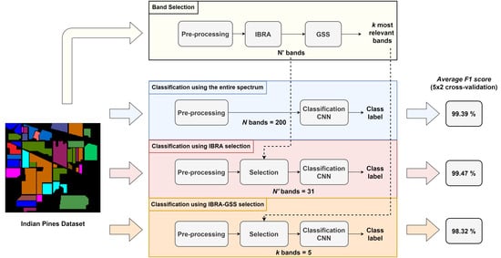
Along with simplifying the hyperspectral data cubes, our IBRA method can be used as part of a novel two-step hybrid feature selection process. The first step applies IBRA to find a reduced set of independent representative bands; then, it applies our proposed wrapper-based method called greedy spectral selection (GSS) to select a user-defined number of spectral channels, as depicted in Figure 1. GSS ranks the candidate bands according to their information entropy to obtain an initial selection of bands, which is used to train a classifier that evaluates the effectiveness of the given selection of bands based on the achieved classification performance. Then, we remove from the selection the band that shows the most severe indication of multicollinearity and repeat the process by considering the next band with the highest information entropy, verifying if the classification performance improves. As such, GSS aims to maximize the discrimination between classes and preserve their spectral uniqueness. This band selection process is implemented as a part of achieving our goal of designing low-cost, high-accuracy MSI systems for various applications. That is, given a classification problem, our method allows us to select a user-defined number of salient wavelengths from an HSI dataset that can then be used for MSI while maintaining or improving the accuracy of the original HSI-based system.
Furthermore, we explore the applicability of IBRA in combination with other dimensionality reduction methods besides the various feature selection methods. Specifically, we propose a feature extraction framework whose first step aims to remove the spectral redundancy by using IBRA. The second step consists of applying any desired dimensionality reduction method on the IBRA-selected set of spectral bands to obtain a new representation with the desired number of dimensions or feature channels. Thus, the structure of the proposed framework is similar to that shown in Figure 1, but including a dimensionality reduction method (e.g., principal component analysis) instead of the GSS block. In this work, we show experimental results for this framework considering both a supervised and an unsupervised feature extraction method for the second step. Our results show that our feature extraction framework yields better or competitive results in comparison to several alternative feature selection methods in the context of hyperspectral image classification.
This paper is an extension of work originally presented at the International Joint Conference on Neural Networks (virtual event, July 2021) [14]. Extensions include an extensive set of experiments that allow for a broader analysis of the behavior of the proposed band selection method. In particular, we include an additional hyperspectral image dataset for our experiments and comparisons to two recently published band selection methods. We also present the results of new experiments focused on testing performance using different dataset sizes (i.e., 100%, 75%, 50%, 25%) to evaluate the impact of data quantity on the effectiveness of our method. In our previous paper, we showed experiments selecting six and ten bands from a hyperspectral dataset used for herbicide resistance classification; here, we include results using eight bands as well in order to evaluate the tradeoff between the number of bands and classification performance more effectively and to explain the advantages of our proposed methods under different scenarios. Finally, we extend the use of our IBRA method to include feature extraction and show how a feature extraction method behaves in comparison to feature selection in hyperspectral image classification.
Our specific contributions are summarized as follows:
- We propose a filter-based method called interband redundancy analysis (IBRA) that works as a preselection method to remove redundant bands and reduce the search space dramatically;
- We present a two-step band selection method that first applies IBRA to obtain a reduced set of candidate bands and then selects the desired number of bands using a wrapper-based method called greedy spectral selection (GSS);
- We show that IBRA can be used as part of a more general two-step feature extraction framework where any dimensionality reduction method can be applied following IBRA to obtain the desired number of feature channels;
- Since one of the objectives of this work is to aid in the design of multispectral imaging systems based on the wavelengths recommended by a band selection method, we also present an extensive set of experiments that use the original hyperspectral data cube to enable simulating the process of using actual filters in a multispectral imager.
The remainder of this paper is structured as follows: In Section 2, we provide a brief review of previous related work performed with feature extraction and feature selection methods in the context of hyperspectral image classification. Section 3 provides further details about the hyperspectral image datasets used in this work, as well as how we preprocessed the data for our experiments. In this section, we also describe our IBRA and GSS algorithms and explain how they are used for dimensionality reduction. Section 5 discusses the experimental results that are presented in Section 4. Finally, Section 6 offers concluding remarks.
2. Related Work
Working with hyperspectral images often benefits from applying dimensionality reduction techniques as a preprocessing step in order to avoid unnecessarily high computational complexity and to reduce redundancy of the data. Dimensionality reduction techniques not only reduce the inherent computational cost and relax the need for advanced hardware requirements for processing the data, but they also combat the “curse of dimensionality” [15,16]; i.e., the fewer the training samples, the worse the performance of an HSI classifier when the dimensionality of HSI data (the number of features) increases [17]. Dimensionality reduction techniques rely on feature extraction or feature selection approaches; the former apply linear or nonlinear transformations to extract specific features from the original data, while the latter select the most useful subset of the features of the data without transforming them.
Feature extraction methods can be subdivided into two classes: unsupervised and supervised. Among unsupervised methods, principal component analysis (PCA) and its variants (e.g., folded-PCA and kernel PCA) are some of the most commonly used methods to remove spectral redundancy and reduce the dimensionality of the raw data [18]. Nevertheless, theoretical arguments and experimental evidence of the ineffectiveness of PCA for hyperspectral feature extraction have been presented [19]. According to this, PCA should not be used as a preprocessing step to solve small-sample-size problems as there is evidence that class separation deteriorates after PCA transformation.
Other unsupervised methods are based on independent component analysis (ICA) and its variants (e.g., kernel ICA and Random Fourier Feature-ICA) [20]. Alternatively, supervised methods such as Fisher’s linear discriminant analysis (LDA) [21,22] or partial least squares discriminant analysis (PLS-DA) [23] are used widely for hyperspectral feature extraction. More recent feature extraction methods apply local manifold learning to find nonlinear embeddings that are used to project the data into lower-dimensional spaces. For instance, Hong et al. [24] proposed a robust local manifold representation that incorporates a hierarchical neighbor selection that aims to mitigate multicollinearity in the local manifold space. Moreover, the computed weights are designed to jointly embed spectral and spatial information. Feature extraction methods can also be applied with the objective of improving data quality. In that sense, Zhuang et al. [25] proposed a robust hyperspectral denoising technique that implements low-rank representations in order to project the data into lower-dimensional spaces while reducing the impact of noise.
On the other hand, feature selection methods select a subset of spectral bands without modifying the data or projecting it into a new basis. In other words, the aim of a hyperspectral band selection method is to identify which spectral wavelengths are most responsive or relevant for a particular classification task without modifying the data. Additionally, identifying a reduced subset of relevant spectral bands allows for a better understanding of the optical properties of the materials and provides information that is useful when designing cheaper task-specific multispectral imagers.
There exists four types of feature selection methods: filter-based, wrapper-based, hybrid, and embedded. Filter-based methods select bands based on various statistical tests that assess the correlation between each band and the outcome variable or among other bands [26,27]. Wrapper-based methods, on the other hand, rely on a learning model to evaluate the suitability of a given set of bands. Hence, the problem becomes a search problem, which is computationally more expensive than filter-based methods [28,29]. In order to avoid an exhaustive search, hybrid methods have been developed. They use a filter-based method as a first step to select some relevant bands; then, a wrapper-based method is used to make the final selection [16,30]. Finally, embedded methods use learning models that internally select the most relevant features during the training phase [31,32]. Below, we provide a brief review of previous related works corresponding to the aforementioned types of feature selection methods.
Given the potential benefits of feature selection, several methods have been proposed for hyperspectral image classification. In this context, some feature extraction methods can be adapted for filter-based feature selection. For example, Chang et al. [33] presented a joint band-prioritization method based on PCA where the spectral bands are ranked according to their variances. PLS-DA can also be adapted into a feature selection scheme using the resulting regression coefficients from full spectra to identify the most influential wavelengths [34,35].
Some filter-based methods analyze the statistics of the data and heuristically estimate a scoring index for each feature. For instance, [36] employed a filter feature-selection algorithm based on minimizing a tight bound on the Vapnik-Chervonenkis (VC) dimension [37]. Ranking-based methods are one of the most common filter-based feature selection methods; these methods estimate the importance of each spectral band using such metrics as the variance inflation factor (VIF) [38] in order to select the top-ranked bands. We will use the idea of calculating the VIF value to measure collinearity, but the spectral bands will not be ranked based on this simple measure alone. Another example of a ranking-based method is the fast density-peak-based clustering (FDPC) method proposed by Rodriguez et al. [39]; it ranks each band according to its ability to become a cluster center, which is measured using two factors: local density and distance from points of higher density. These factors are calculated using a similarity matrix based on Euclidean distance. Similarly, Xu et al. [40] constructed a similarity matrix based on structural similarity (SSIM) that is used to calculate two measures called average similarity and significant dissimilarity to evaluate the ability of each band to become a cluster center. Then, it ranks the bands according to the product of these two measures so that the top-ranked bands are selected.
Other methods estimate the relevance of each band as part of an optimization approach. For instance, Medjahed and Ouali [41] formulated the feature selection problem as a combinatorial optimization problem where feature relevance is measured by mutual information. Furthermore, Wang et al. [27] proposed an optimal clustering framework (OCF) that searches for an optimal band partition. Here, the clustering strategy is to evaluate the contribution of each cluster and then sum the contributions as a measure of the whole clustering result. After obtaining an optimal partition, the method ranks each band within a cluster according to a selected measure (e.g., information entropy) and selects those with higher rank values. In subsequent work, Wang et al. [26] proposed a fast neighborhood grouping method for hyperspectral band selection (FNGBS) that uses a neighborhood band grouping approach to partition the data into several groups based on Euclidean distance. After partitioning the data, the method ranks the bands within each group according to the product of local density and information entropy in order to obtain the most relevant and informative band for each cluster.
Recently, wrapper-based feature selection approaches based on genetic algorithms have gained more attention [28,42,43]. For instance, a recent method for bandwidth selection is known as histogram assisted genetic algorithm for reduction in dimensionality (HAGRID) [29]. This method maintains a population of index vectors identifying a specific number of wavelengths and fits a Gaussian mixture model to the converged population to identify the main wavelengths with their associated filter bandwidths.
Alternatively, some embedded-based approaches have been proposed in the context of deep learning. Taherkhani et al. [31] proposed regularizing the convolutional filters of the first layer of a convolutional neural network (CNN) using a group least absolute shrinkage and selection operator (LASSO) algorithm in order to sparsify the redundant spectral bands. Similar attempts, although they are not explicit feature selection methods, have been carried out in works such as [44,45], where a spectral-wise attention mechanism in the form of a fully connected layer is applied to the inner convolutional layers of the network with the objective of emphasizing informative spectral features and suppressing less useful spectral features. Furthermore, the use of saliency maps have gained popularity due to their ability to estimate which features (i.e., pixels) are more relevant for a model [46,47]. For example, Nagasubramanian et al. [48] adapted the concept of spatial saliency maps to an HSI classification scheme in order to estimate the relative importance of each wavelength given a specific class.
3. Materials and Methods
3.1. Dataset Descriptions
In our experiments, we used an in-greenhouse controlled HSI dataset of kochia leaves in order to classify three different herbicide resistance levels. We also used two well-known remote sensing HSI datasets: Indian Pines (IP) [49] and Salinas (SA) [50].
The Kochia dataset consists of images of the weed kochia (Bassia scoparia), which is considered one of the most problematic weeds in small grains and broadleaf crops such as soybeans and sugar beets [51,52,53]. This dataset was collected and analyzed by Scherrer et al. [1] with the aim of learning to differentiate between three different classes of herbicide resistance of this weed: (1) herbicide-susceptible, (2) glyphosate-resistant, and (3) dicamba-resistant, where glyphosate and dicamba are two components commonly found in commercial herbicides [53]. It is important to note that the difference between these three classes is imperceptible using standard color digital cameras that collect data for three bands in the visible spectrum of light (red, green, and blue), which justifies the need of using hyperspectral or multispectral imaging systems. The images were captured using a Resonon Pika L hyperspectral imager with 300 spectral channels across a spectral range of 387.12 nm to 1023.50 nm, resulting in a spectral resolution of approximately 2.12 nm. The kochia samples were illuminated using diffuse sunlight in a greenhouse setting. A total of 76 hyperspectral images of kochia with varying ages and spatial resolutions were captured at the Montana State University Southern Agricultural Research Center (SARC). Each image contains three kochia leaves of the same herbicide resistance class with a height of 900 pixels and width ranging from 700–1200 pixels.
The Indian Pines dataset [49] is an aerial -pixel image of the Indian Pines site in Northwestern Indiana. It was acquired in 1992 using the Airborne Visible/Infrared Imaging Spectrometer (AVIRIS) sensor [54], and it originally had 224 spectral bands in the wavelength range 400–2500 , resulting in a spectral resolution of approximately 9.5 nm. The number of bands was first reduced to 220 after removing four damaged bands without information (i.e., all of their pixels were zero value) [49], and then to 200 after removing 24 noisy bands and bands covering the region of water absorption corresponding to the wavelengths (1333–1373 ), (1789–1893 ), and (2499 ) that correspond to the band indices (104–108), (150–163) and 220, as recommended by Tadjudin and Landgrebe [55]. The data are divided into 16 classes containing agriculture, forest, and other natural perennial vegetation.
Similarly, the Salinas dataset [50] is a -pixel aerial image of Salinas Valley, California, that was gathered in 199 using the same AVIRIS sensor as Indian Pines. Bands in the same wavelength ranges as Indian Pines were removed; however, in this case, they correspond to the following band indices: (108–112), (154–167) and 224. Thus, only 204 spectral bands are used. It is divided into 16 classes containing vegetables, vineyard fields, and bare soil.
3.2. Data Preprocessing
Each of the 76 collected images in the Kochia dataset contains a reflectance standard and three kochia leaves that correspond to the same herbicide resistance class. The white panel shown on the left side of each image in Figure 2 corresponds to the reflectance standard, a 99% reflectance Spectralon panel, which is commonly used as a Lambertian calibration reference. These images were captured by the Pika L hyperspectral imager in raw digital numbers, meaning the image data required preprocessing prior to analysis. For our experiments on the Kochia dataset, we converted the raw digital numbers to reflectance values using the Spectralon panel as the reflectance reference.
The first step of the reflectance correction was to select the pixels in the image that contain the Spectralon reflectance target. Next, we averaged the values of all pixels within the selected region at each spectral band, leaving us with a single, averaged digital number for each spectral band (where N represents the total number of spectral bands) denoted as . Consequently, we obtained a digital number representing 99% of the reflected light for each spectral band. Finally, we calculated the spectral reflectance at the i-th pixel of the n-th spectral band, , as follows:
where represents the digital number value captured at the i-th pixel of the n-th spectral band, represents the dark current or background signal generated through sporadic electron generation in the imager’s sensor, and represents the reflectivity of the reflectance target.
From the calibrated images, we extracted 6316 -pixel overlapping patches (Figure 2c). Once extracted, we reduced the number of spectral bands within each patch from 300 to 150 by averaging adjacent pairs of bands, which can be interpreted as spectral binning, where the resulting spectral resolution of each band was modified from approximately to . Thus, the final shape of this preprocessed dataset is pixels.
Given that one of the goals of this work is to aid in the design of multispectral imaging systems, we note that decreasing the overall spectral resolution is unlikely to affect our results, as it is unlikely that optical filters with a bandwidth less than 20 will be considered. Hence, this process gives us an upfront reduction in dimensionality that greatly reduces the potential overfitting impact in our following analysis without overly constraining the design parameters of a multispectral imager. In addition, averaging consecutive bands has a smoothing effect that helps to combat possible noise in some spectral bands.
However, we used a different process for the IP and SA datasets. As described in Section 3.1, these datasets consist of single large images, meaning that we had to divide them into small patches so that each patch represents one class. In this case, we extracted -pixel patches around each pixel with an assigned label. From the IP and SA datasets, we extracted 10,249 and 54,129 patches, respectively. Hence, the size of the preprocessed IP dataset is 10,249 pixels while that of the preprocessed SA dataset is 54,129 pixels.
3.3. Interband Redundancy Analysis
Our first contribution consists of having developed a method called interband redundancy analysis (IBRA) that selects a subset of representative spectral bands from the original data cube aiming to reduce the interband redundancy. IBRA is a filter-based selection method that iteratively calculates the variance inflation factor (VIF) [56] between pairs of bands in order to determine how correlated they are; that is, to verify the presence of collinearity between them.
To calculate the VIF value between two bands, and , we built an ordinary least squares (OLS) regression model that takes one of the bands as the independent variable () and the other as the dependent variable (). Then, we used the R-squared (coefficient of determination) value from the resulting model, , to calculate the VIF value as follows:
VIF values range from 1 upwards. The higher the VIF value, the more there is the risk of collinearity. If two bands are collinear, they explain the same variance within the dataset and can be considered to be redundant. We will consider VIF values greater than a threshold as representing the presence of collinearity between two spectral bands. In the literature, the recommended values of are between 5 and 10 [57,58], so we test different values of to observe how the classification performance is affected by this threshold and to choose the best for a given classification task.
Some methods, such as that proposed by Castaldi et al. [38], use the VIF metric to perform a stepwise selection process where the bands that show a VIF value greater than a threshold (i.e., bands that show a high risk of multicollinearity) are removed from the selection. Our approach is novel and distinct in that we use the VIF metric as part of a preselection step, assessing the collinearity degree between each band and its local neighbors iteratively in order to find independent salient bands that are suitable cluster centers.
Our IBRA preselection method first analyzes each spectral band with spectral index to calculate the minimum number of bands we need to move away to the left side from it in order to find bands sufficiently different from band , denoted as . Similarly, we calculated the minimum number of bands we need to move away to the right side from band in order to find bands sufficiently different from band , denoted as (see Algorithm 1). From this, we assumed that all the bands within the interval are similar to and form a possible cluster.
We considered that a suitable cluster center should represent the bands that are on the left side of the cluster in a similar way that it represents those on the right side; therefore, we calculated the difference to quantify the suitability of band to become a cluster center, where low values of indicate better suitability. Take Figure 3 as an example. Here, () is more suitable than () to be considered a bandwidth center because it is similar to both the left and right sides, so it better represents the bands within the interval . Recall that there exists a strong correlation between bands with close wavelengths [27], which means that the more distant two bands are, the more different their spectral information is.
Next, we analyzed how the differences were distributed across the spectrum. This distribution was used to find clusters with similar bands and their corresponding cluster centers. Figure 4 shows the distribution of the variable for the Kochia dataset given different thresholds . From this, we observed that each distribution consisted of a series of “V” patterns. In this context, a local minimum—the center of a “V” pattern—represents a salient band that explains the variance within the dataset in a way similar to its neighbors. Even though all the bands within a “V” pattern are similar, the band at the leftmost position is more similar to those bands on the left side of the cluster. Similarly, the band at the rightmost position of the “V” is more similar to those bands on the right side of the cluster, while the band corresponding to the local minimum is similar to both sides, acting as a centroid. In general, we kept the bands corresponding to a local minimum in the n vs. plot and remove the rest since they are assumed to be redundant. We considered only local minima where ; otherwise, they will not be suitable bandwidth centers.
The entire IBRA process is described in Algorithm 1 and Figure 5. Here, getVIF() calculates the VIF value between bands and . Note that ; therefore, in order to avoid re-calculations and make the algorithm more efficient, we construct a symmetric matrix that stores the pre-computed VIF values between pairs of bands. Furthermore, is a function that retrieves the position of the local minima of the vector d. Hence, the algorithm returns a vector called preselection, which is a set of numbers (where ) representing the indices of the preselected spectral bands. It is worth mentioning that the number of preselected bands is not known a priori and depends on each dataset and the selected VIF threshold .
| Algorithm 1 Calculating the interband redundancy. |
|
3.4. Band Selection Using Pre-Selected Bands
Our second contribution was the development of a two-step hybrid band selection method: First, it uses IBRA to obtain a set of independent candidate bands from the original spectrum, as we showed in Section 3.3. Then, it employs a wrapper-based method to select the best combination of bands given the desired number of bands k (whose indices are denoted by ) from the set of available candidate bands preselected by IBRA (whose indices are denoted by ) instead of the entire set of spectral bands, which greatly reduces the search complexity. We call this process greedy spectral selection (GSS).
The GSS process starts by ranking each candidate band , where , according to some criterion. In this work, we used information entropy to calculate an initial relevance score for each spectral band. The three datasets used in this work were acquired using a bit depth of 14 bits, allowing us to interpret a spectral band as a discrete random variable. The entropy of band , , conveys the average level of information inherent in and is defined as follows:
where is the probability mass function of random variable z, and is the space that encompasses all the possible values that can occur in the spectral band .
Here, it is important to highlight the difference of our method with respect to other band selection methods that use information entropy as a ranking measure, such as those proposed by Wang et al. [26,27]. In particular, those methods use an optimization approach to group the data into k clusters of similar bands. Then, they use information entropy to find the most representative band from each cluster (i.e., the band with the largest amount of information) to obtain a final selection of k bands. Our approach is distinct in two aspects: First, when using IBRA, we already picked the most representative band from each cluster (defined as a local minimum in the n vs. plot, as shown in Figure 4). Then, we ranked the preselected bands based on information entropy in order to select a subset of k bands. Thus, initially, consists of the indices of the top-k candidate bands of with the greatest entropy. The second aspect is that, while other methods use information entropy to obtain a final selection of bands directly, we used it to obtain an initial selection that will be refined further using a greedy algorithm based on a multicollinearity analysis.
We note that collinearity does not exist between pairs of candidate bands obtained by the IBRA preselection process because the calculated VIF value between two cluster centers must be lower than a given threshold . However, it is possible that three or more bands are highly correlated—a phenomenon known as multicollinearity [57]. In that case, we checked for the presence of multicollinearity within the k selected spectral bands the same way as described in Section 3.3 with collinearity; that is, taking one band at a time, considering it as the dependent variable while considering the rest of the bands as the independent variables, and calculating its corresponding VIF value.
With this, after obtaining an initial set of k selected bands based on information entropy, GSS employs the following greedy algorithm (see Algorithm 2). First, we calculated the average classification performance (F1 score) when using the current k selected bands. To do this, we performed a -fold cross-validation using a convolutional neural network (CNN) classifier (see Section 3.5) and calculated the average F1 score obtained on the 10 validation folds. Then, after calculating the VIF value for each of the currently selected bands, we removed the one with the greatest VIF value and consider the next available band with the greatest entropy. With this new subset of k bands, we performed a new -fold cross-validation process to determine if the average classification performance had improved. If so, we considered the current selection of k bands as the current best selection and updated the indices of . We repeated this process until there were no more available bands. Finally, we selected the combination of bands that showed the best classification performance.
| Algorithm 2 Greedy spectral selection. |
|
Figure 6 depicts the process of selecting bands for the Kochia dataset from the set of 17 band candidates obtained using IBRA with a VIF threshold of 10 (see Figure 4b). Then, in the first iteration of GSS, the first six bands selected are those with the highest information entropy values; for example, those with indices . With this selection of bands, we performed -fold cross-validation training a CNN and obtained an average F1 score of 92.49%. Then, we determined that the band with index 64 had the highest VIF value (i.e., 86.8), which means that its variance could be explained well using the other five bands. For this reason, this band was removed from the selection and the next available band (i.e., the band with index 43) was considered in the second iteration. We show the results obtained after six iterations only given that the following iterations could not achieve better classification performance scores. Therefore, the best selected bands were found at the fifth iteration and their indices were .
The GSS algorithm is presented in Algorithm 2 and Figure 7. Note that it selects the indices of the best k bands from a list of candidate band indices . Function getEntropy() returns the entropy value of each of the candidate bands with indices . Then, .sort(key = H) sorts the elements of with respect to their corresponding entropy values in nonincreasing order. Function getVIFMulti() returns a list with the VIF value for each band in . Next getMax(l) returns the position where the maximum value in a list l was found. Finally, the performance of the currently selected bands was evaluated using trainSelection(), which returns the average F1 score obtained using the bands with indices and -fold cross-validation.
3.5. Convolutional Neural Network Architecture
The type of classifier we used for the GSS process to evaluate the appropriateness of a given selection of spectral bands (line 6 in Algorithm 2) is a CNN. Preliminarily, we experimented with other types of classifiers to use in the GSS process; specifically, support vector machines, random forests, and feedforward neural networks. However, these approaches showed slow convergence rates and poor classification performance in comparison to our CNN, despite being a more complex model. For this reason, we continued to use CNNs over the other types of classifiers.
All the classifiers used in this work are CNNs that use a modified version of the Hyper3DNet architecture [59], which is a 3D-2D CNN architecture specifically designed for HSI classification problems using a reduced number of trainable parameters. The original Hyper3DNet architecture consists of two main modules: a 3D feature extractor and a 2D spatial encoder. The 3D feature extractor uses a sequence of 3D convolutional layers with filters that analyze not only spatial neighborhoods but also spectral neighborhoods while maintaining spatial resolution. Then, the 2D spatial encoder progressively reduces the spatial resolution using 2D separable convolutional layers, which are used due to their ability to reduce the number of trainable parameters and computational burden while improving the classification performance [60,61]. Experimental results demonstrated relative superiority of this architecture over state-of-the-art architectures.
The modified CNN architecture that we used in this paper, referred to as Hyper3DNet-Lite, is a simplification of the original Hyper3DNet architecture. The difference with the original architecture is that its 3D feature extractor consists of two 3D convolutional layers instead of a densely connected block with four layers; additionally, its 2D spatial encoder has three layers instead of four. The Hyper3DNet-Lite architecture used for the Kochia dataset is detailed in Table 1, where N denotes the number of spectral bands in the input, “SepConv2D” denotes a 2D separable convolutional layer, and “ReLU” denotes a rectified linear unit activation layer (where . The only difference with the network used to process the IP and SA datasets is that, since the input image is smaller ( pixels), the stride used in the last two “SepConv2D” layers is instead of to avoid dimensionality inconsistencies.
Another difference of our Hyper3DNet-Lite with respect to the original Hyper3DNet is that, after the last “SepConv2D” layer, we used a “GlobalAveragePooling” operation instead of a “Flatten” operation. For example, for the case of the network shown in Table 1, we transformed our 3D tensor with dimensions pixels into a 1D vector with 256 elements by averaging the 49 values from each channel. Conversely, if we were to use a flattening operation, we would obtain a 1D vector with 12,544 elements. This relaxes the need of using an intermediate fully connected layer to reduce the dimensionality of the tensor before the final classification layer; thus, we avoided using an excessive number of trainable parameters.
The simplified architecture of the Hyper3DNet-Lite network becomes especially suitable for datasets that use just a few spectral bands, given that these datasets often do not require models with a high level of complexity to process them, unlike those datasets that use all the available spectral bands. In this way, we avoided overparameterization, which results in our models being less prone to overfitting.
3.6. Multispectral Imager Design
A spectral band is determined by its wavelength center and its spectral resolution; that is, an imager captures the reflected light in a given band around its center wavelength within a range determined by its spectral resolution. The method described in Section 3.4 was used to select the most relevant spectral bands from the original hyperspectral data cube and, as a consequence, their wavelengths. Knowing which wavelengths are more useful for a given application allows us to discard the information captured at different wavelengths, thus reducing storage requirements. However, this knowledge also allows for the design of a compact multispectral imager that would be used instead of a full hyperspectral imager. Hence, to test our hypothesis that we can use our method to provide the specifications needed to design a multispectral imager, we assessed classification performance with a simulated multispectral imager by using the original hyperspectral data cube and simulate applying optical filters to capture data from an imager that would use our selected wavelengths.
The bandwidth of the simulated multispectral filters is set to be equivalent to the bandwidth encompassed by five bands, which is equivalent to 21 for the case of the Kochia dataset, and 50 for the case of the IP and SA datasets. These are commonly available optical filter bandwidths. To obtain the reflectance measured by the simulated multispectral sensor, we generated k Gaussian distributions, one for each of the selected bands, taking the spectral wavelengths selected by a band selection method as the centroids. The spread of the generated Gaussian curves is proportional to the filter bandwidth. In particular, the full-width at half-maximum (FWHM) of the curve was set to be equal to the bandwidth [29]. The FWHM is defined based on the standard deviation of the curve as . Then, the simulated multispectral reflectance measurement was obtained by multiplying the original hyperspectral data cube by the corresponding Gaussian distribution generated for each band, then integrating under the resulting response curve to obtain a single reflectance value. This process was repeated for each of the k Gaussian distributions.
3.7. Feature Extraction Framework
Feature extraction approaches project the N original spectral bands into a new representation basis of features (where ). As such, transformed features can no longer be interpreted as spectral bands. In other words, we lose data interpretability. However, in some cases, feature extraction methods may present some performance advantages over feature selection methods. For example, projecting the data into a new basis with reduced dimensionality based on PCA helps to remove redundancy while trying to explain the original variance of the dataset. Conversely, feature selection methods simply discard the information of the bands that were not selected. Therefore, a classifier trained on transformed features that explain most of the original variance of the dataset might perform better than a classifier trained on selected bands, considering that the discarded bands did not contain trivial information.
We propose generalizing our method described above into a two-stage feature extraction framework. First, we applied IBRA to remove redundant bands; then, we can use any feature extraction method to obtain the desired number of feature channels k. In this work, we demonstrate the pipeline using two types of feature extraction methods: unsupervised and supervised. We chose PCA as the unsupervised method and denote the resulting instance as IBRA-PCA. In addition, we used PLS-DA as the supervised method; here, we used the class labels of the dataset to maximize the class separation within the reduced space. This instance is denoted as IBRA-PLS-DA.
4. Experimental Results
In this section, we present the experimental results for each step of our proposed methods and analyze their performance in comparison to other dimensionality reduction methods. For the sake of consistency and fairness, we used the same configuration for all the networks trained in our experiments, including those used during the GSS process. That is, we used the same network architecture (i.e., Hyper3DNet-Lite), optimizer, and batch-size. While this strategy does not guarantee the best possible results, it allowed us to compare the behavior of different band selection methods under the same conditions. All CNNs were trained using the Adadelta optimizer [62], which is a gradient descent method based on an adaptive learning rate, so that there is no need to select a global learning rate manually. The mini-batch size was set to 128. The last layer of the CNNs used a softmax activation function, and we employed a categorical cross-entropy loss function.
We applied -fold stratified cross-validation to train and evaluate all networks. That is, we randomly divide our datasets into two equally sized folds so that one fold works as the training set and the other as the validation set, train again with the roles of these folds reversed, and then repeat this process four more times. Furthermore, stratification indicates that each fold has the same proportion of samples of a given class. Note that z-score normalization (mean equal to zero and standard deviation equal to one) was applied onto each spectral band of each training set while the exact same scaling was applied to their corresponding validation set. In order to analyze the behavior of our models, we calculated four metrics by aggregating the results on all ten of the validation sets: overall classification accuracy, macro-average precision, macro-average recall, and macro-average F1 score. The source code and datasets are available online (Codebase: https://github.com/GiorgioMorales/HSI-BandSelection.git, accessed on 5 July 2021).
4.1. Training with Preselected Bands Alone
Previously (Figure 4), we showed some examples of applying the preselection method using IBRA on the Kochia dataset using three different VIF thresholds (12, 10, and 8), which reduced our search space from 150 bands to 19, 17, and 16 bands, respectively. Table 2 gives the number of preselected bands for the Kochia, IP, and SA datasets when using IBRA with a VIF threshold of 10 (); it also gives the average performance for the four metrics and corresponding standard deviations using the Hyper3DNet-Lite network when training on the full hyperspectral spectrum and only the preselected bands. The number of parameters required to train each network is reported in the last column.
4.2. Greedy Spectral Selection
From Figure 4, we notice that different VIF thresholds can lead to slightly different selections of candidate bands. In general, the lower the VIF threshold, the more distinct two bands have to be to be considered noncollinear. Exactly how large this threshold needs to be is not clear. If it is too large, we may end up including too many candidate bands that do not represent suitable bandwidth centers. On the other hand, if it is too small, we may discard bands that could have been useful for the classification task. For that reason, we applied IBRA using different VIF thresholds so that we obtained a set of preselected bands for each of them. Then, we applied GSS on each set of candidates to select the desired number of bands k. Finally, we selected the classifier that achieved the best classification performance based on the mean F1-score obtained after a -fold cross-validation.
For the Kochia dataset, we considered six, eight, and ten bands in order to evaluate the tradeoff between the number of bands and classification performance. For the IP and SA datasets, we selected only five bands. This is because we found that the ease of training these datasets when using yielded to high-performance metrics (>99% accuracy) no matter which feature selection method was chosen. That is, the lack of sufficiently distinct results prevented us from being able to evaluate the existence of any performance difference among the various methods, which is why selecting more than five bands from these datasets was not considered appropriate for this work. In addition, for each dataset, we experimented with different dataset sizes (i.e., 100%, 75%, 50%, and 25%) to evaluate how consistent the band selection results as the data availability changes.
For the Kochia dataset, when selecting six bands (), the best results were obtained using a VIF threshold of ten (), and the wavelengths of the selected bands (in ) were for each of the four dataset size variations. Equivalently, the indices of the selected bands were . When selecting eight bands (), the best results were obtained using a VIF threshold of when using 100%, 50%, and 25% of the dataset and when using 75% of the dataset. In the four cases, the difference between the classification performance obtained using , , and is not statistically significant, so we considered the three options equally as good. Therefore, in this work, we simply chose the bands selected using since it achieved slightly higher performance metrics in three out of the four dataset variations. Hence, the wavelengths of the selected bands were () with indices .
When selecting ten bands (), the best results were obtained using a VIF threshold of when using 100% and 50% of the dataset, and when using 75% and 25% of the dataset. The wavelengths of the bands selected for were ()—with indices —and the only difference with respect to the bands selected for was the selection of the wavelength —which corresponds to the band index 45—instead of —which corresponds to the band index 43. Table 3 shows the performance using IBRA and GSS on the full Kochia dataset for different VIF thresholds () when selecting six, eight, and ten bands. The bold entries in these tables represent the best VIF threshold and average F1 score.
For the IP dataset, the best results were obtained using a VIF threshold of ten () and the wavelength of the selected bands were (i.e., with band indices ) for all four dataset size variations except when we used 50% of the dataset, where the best VIF threshold was nine () and the wavelength (band index 46) was selected instead of the wavelength (band index 39). Table 4 shows the performance using IBRA and GSS on the full IP dataset.
For the SA dataset, the best classification performance was obtained using a VIF threshold of when using 100% and 75% of the dataset. The wavelength of the selected bands were (), which correspond to the indices of the corrected SA dataset after discarding the 20 water absorption bands (see Section 3.1). When we reduced the dataset size, different VIF thresholds were selected. Specifically, when we used 50% of the dataset, the best VIF threshold was six (), and we selected the wavelengths (index 20) instead of (index 37), (index 91) instead of (index 92), and (index 174) instead of (index 175). Furthermore, when we used 25% of the dataset, the best VIF threshold was seven (), and we selected the wavelength (index 174) instead of (index 175). Similar to what happened with the Kochia dataset when selecting eight bands, the classification performance obtained using , , and was not statistically significant, so we considered the three options equally as good; however, in this work, we chose to use the bands selected using , as it yielded slightly better performance metrics in two out the four dataset variations. Table 5 shows the performance using IBRA and GSS on the full SA dataset.
4.3. Comparative Results
We compared our IBRA-GSS method to four other band selection methods: OCF [27], HAGRID [29], SR-SSIM [40], FNGBS [26], and PLS-DA [63]. For OCF, we used the normalized cut criterion as the objective function along with information entropy as the ranking method, given that this setting showed the best performance. For HAGRID, we used a grid search to choose the following hyperparameters: a crossover rate of 0.25, a mutation rate of 0.05, a tournament size of 5, a population size of 1000, and 300 iterations. For SR-SSIM, we used a window size of 3 for the SSIM index algorithm to construct a hyperspectral similarity matrix, as it achieved the best performance. For FNGBS, to calculate the number of shared neighbor elements between two bands, we considered a nearest neighbor of two elements. Finally, we adapted PLS-DA for feature selection by sorting the coefficients obtained by PLS-DA in order to select the top-k bands. We also compared our IBRA-GSS method to our IBRA-PCA and IBRA-PLS-DA methods to analyze the behavior of feature extraction methods in front of a feature selection method.
To assess the effectiveness of the dimensionality reduction methods, we compared the performance of eight Hyper3DNet-Lite CNNs, each trained on the features selected or extracted by the eight methods. This comparison was carried out using the same network architecture, hyperparameters, and other configurations for all of the methods. Finally, to determine if the difference in performance scores was statistically significant, we performed a paired t-test and a paired permutation test using the F1 scores at the level.
The method comparison is shown in Table 6 for the Kochia dataset, Table 7 for the IP dataset, and Table 8 for the SA dataset, with the best performing metrics highlighted in bold. Here, the first row of each method represents the results obtained after training a model using the original selected bands (identified as “original band selection”), while the second row represents the results obtained after using simulated filters that take the position of the selected bands as their central wavelengths (identified as “multispectral filter simulation”), as explained in Section 3.6. Additionally, we chose the average F1 score to compare the results of all the methods graphically in Figure 8. The simulated filters used for the Kochia dataset were 20 , while for the IP and SA datasets, they were 50 . Note that the feature channels extracted by IBRA-PCA and IBRA-PLS-DA cannot be interpreted as spectral bands; thus, we could not apply the “multispectral filter simulation” approach directly on them. Instead, we applied a Gaussian transformation on the IBRA-selected bands to simulate filters that take the position of the preselected bands as their central wavelengths; then, we used PCA or PLS-DA on the transformed bands to obtain the desired number of feature channels.
Additionally, Table 9 shows the resulting p-values of the paired t-tests and paired permutation tests performed between IBRA-GSS and the other compared methods when selecting six, eight, and ten bands from the Kochia dataset. Similarly, Table 10 shows the results of the statistical significance tests between IBRA-GSS and the other methods when selecting five bands from the IP and SA datasets. In both cases, the upward-pointing arrow (↑) indicates that IBRA-GSS performed significantly better (i.e., p-value ), the downward-pointing arrow (↓) indicates that the compared method performed significantly better than IBRA-GSS, and the equal symbol (=) indicates that the difference between IBRA-GSS and the compared method is not statistically significant (i.e., p-value ). According to both the t-test and the permutation test, our IBRA-GSS method performed significantly better than the other five band selection methods in each of the cases; however, it did not perform better than IBRA-PLS-DA nor IBRA-PCA (except for the “original band selection” case) when selecting eight or ten bands from the Kochia dataset.
We also evaluated how the distribution of the F1 scores resulting from using different dimensionality reduction techniques changes as k changes. To do this, we considered a population that consisted of all the F1 scores obtained by all the methods (i.e., a sample size of 80) on the full Kochia dataset. From this, we show in Table 11 that the overall mean F1 score increases as k increases, while the standard deviation decreases; that is, the F1 scores are more spread out when k is small. We also performed a one-way analysis of variance (ANOVA). In this case, each group consisted of the ten F1 scores obtained by each method. From Table 9, we already know that such statistically significant differences exist, so, as expected, the F statistics obtained for the three values of k are high and their corresponding p-values are quite small (p-value ≪ 0.05), as shown in Table 11. However, notice that the F statistic decreases and the p-value increases as k increases. In other words, as k increases, it becomes less likely that choosing a specific dimensionality reduction technique will cause a significant difference in the resulting average F1 score. This is not surprising, since, by increasing k, we are effectively reinserting what was considered to be overlapping information.
We also tested the four dataset size variations, as explained previously. For example, Figure 9 depicts the performance metrics comparison of the eight methods for the Kochia dataset using four dataset size variations and selecting six, eight, and ten bands. For the three tested datasets, we found that the improvement in performance of our IBRA-GSS method over the other feature selection methods was still statistically significant even when the dataset size was reduced, except when selecting eight bands () from the Kochia dataset and using 25% of the dataset (Figure 9d).
5. Discussion
Our IBRA method is used to cluster the entire spectrum into sets of similar (or collinear) spectral bands and to identify their cluster centers directly. Furthermore, we can interpret these bands as representing a set of influencing spectral bands with wavelengths that are suitable for the design of multispectral filters. These preselected bands explain the variance of their neighbors (i.e., spectral bands that belong to the same cluster) in the original spectrum with a VIF value greater than a threshold ; therefore, keeping them and removing the other bands of each cluster allow us to avoid spectral bands that do not contain useful information for performing classification. That is, our method effectively identifies those spectral bands that carry information for performing classification while discarding redundant spectral bands. Results shown in Table 2 demonstrate that it is possible for a model trained on the subset of spectral bands determined by IBRA to achieve high accuracy values (∼97–99%) while discarding most of the bands, similar to those obtained when using the full spectrum. For example, for the case of the Salinas dataset when using a VIF threshold of 10, we reduced the number of bands from 204 to 14, discarding more than 93% of the bands while decreasing the average F1 score less than 0.2 percentage points, which was also shown not to be significantly different. Thus, we were able to train a CNN classifier that required 80% fewer trainable parameters than a model trained on the full spectrum yet without detriment to its performance.
Our GSS method uses information entropy as a ranking criterion to identify which bands incorporate more information among the bands preselected by IBRA. However, if we need to select at most k bands, the subset of bands with the greatest information entropy values may not be the best selection. For instance, for the Kochia dataset, for , the wavelengths of the bands with the highest entropy values were (); however, line 9 in Algorithm 2 detected strong multicollinearity between bands with wavelengths and in the first iteration (see Figure 6). Rather than using redundant bands, our method selects a more diverse subset of bands if this helps to improve the classification performance.
It is worth noting that, according to the results described in Section 3.4, there does not necessarily have to be a single optimal VIF threshold to find the best set of spectral bands for a given classification task. Instead, more than one value of can lead to the same or similar selection of bands. For example, from Table 5, the only difference that we obtained using with respect to using is that we selected the wavelength (band index 175) instead of (band index 174). Considering that these two bands are contiguous, they explain practically the same variance, so both options are equally as good, which can be verified by observing that their resulting classification performance were very similar. There were other cases where, given two VIF thresholds, the GSS method selected bands that are located in different parts of the spectrum, and yet both options are considered equally as good as there was no statistical difference between their classification performance, as observed in Table 3 when using and .
From Table 6, Table 7 and Table 8, we see that our IBRA-GSS method performed better than the other five band selection methods on the three datasets. The results remained consistent even when considering different dataset sizes except in one case when using the “multispectral filter simulation” approach on the Kochia dataset. In fact, Figure 9 shows that the gap in performance between our method and the others became more noticeable when the dataset size was reduced. In addition, Table 11 shows that the average F1 scores obtained by each method in both approaches are more spread out when selecting six bands than when selecting eight or ten bands (which can be visually verified in Figure 9). This confirms that the fewer spectral bands we select, the harder the band selection task will be; however, multispectral imagers generally become more practical computationally as the number of spectral channels becomes smaller. Thus, the fact that IBRA-GSS consistently outperformed the others when selecting a reduced set of spectral bands makes it the most suitable band selection method for multispectral imager design, at least for the data sets analyzed and the algorithms studied.
With our IBRA-GSS method, the classification performance resulting from the “original band selection” approach was very similar to the performance with the “multispectral filter simulation” approach, unlike some of the compared methods. This can be explained by the way we selected the first band candidates using IBRA. That is, a spectral band corresponding to a local minimum in the plot of spectral index vs. distance (Figure 4) acts as a centroid due to its similarity to the spectral bands located on either side. Therefore, if we take this local minimum as the central wavelength of a multispectral filter, generate a Gaussian distribution around it by considering a standard bandwidth, and integrate under the response curve, then we obtain reflectance values similar to those of the central band. Given that the simulated multispectral filter and the original spectral band present similar information, their classification performance was similar. This is convenient for a multispectral sensor design, as we would like the central wavelength of a filter to be the most representative.
Regarding our tested feature extraction methods, we observe from Table 9 that IBRA-PCA and IBRA-PLS-DA were able to obtain better or competitive results than those obtained by our IBRA-GSS band selection method when using eight () or ten () feature channels from the Kochia dataset. Nevertheless, they could not obtain better performance than IBRA-GSS or other band selection methods when extracting fewer channels. This is due to the fact that PCA tries to explain the total variance of the original features (i.e., the IBRA-selected bands) and PLS-DA tries to explain the maximum variance of the response variable (i.e., maximizes inter-class separability) so that the fewer the number of dimensions we choose in both cases, the worse this explanation is. Conversely, when k is small, our GSS method does not apply a poor transformation on the spectral bands. Instead, it seeks to find a set of original spectral bands that maximize class separability. For the specific case of PCA, we noticed that the performance obtained using the “original band selection” was significantly lower than that obtained using the “multispectral filter simulation” approach. This is because reflectance measures captured by narrow hyperspectral bands tend to introduce a considerable number of outliers and PCA is an outlier sensitive feature extraction technique. On the other hand, the Gaussian transformation applied to simulate multispectral filters has a smoothing effect that reduces outlier noise; thus, improving the classification performance dramatically.
6. Conclusions
Hyperspectral imaging systems capture highly complex data that allow us to extract information that could have not been achieved using only visual spectral bands or spectrometers. However, processing hyperspectral images entails a high computational cost that can be avoided using dimensionality reduction techniques. In that sense, feature extraction techniques are used to transform the data and reduce its dimensionality, which improves the computational efficiency when processing HSIs while avoiding performance degradation derived from the phenomenon known as the curse of dimensionality. Feature selection techniques, on the other hand, help to determine the most relevant wavelengths for a given application, which allows for the design of compact multispectral imagers that could be used in place of hyperspectral imagers. This approach leads to even more significant economic savings, as fewer specialized storage and processing devices are required.
Given these potential benefits, in this paper, we focused on the proposal of a filter-based (IBRA) and a hybrid (IBRA-GSS) band selection method in the context of hyperspectral image classification. Experimental results showed that our IBRA method alone is able to discard up to 93% of the spectral bands and achieve similar classification performance to that obtained using the full spectrum. Therefore, IBRA successfully removes redundant spectral bands while maintaining the most relevant spectral information for a given classification task.
Furthermore, our IBRA-GSS method was proposed as a hybrid selection method that allows for the selection of a specific number of spectral bands k. IBRA-GSS was shown to generally outperform the other competing band selection methods on the three tested datasets even when we reduced the dataset sizes. We also observed that more than one VIF threshold in the IBRA step can lead to the same or similar selection of bands that were found to be equally as effective. This behavior was found to be consistent when the dataset size was reduced.
We also showed how to use our IBRA method as part of a novel feature selection framework. Two variants of this framework were tested, namely IBRA-PCA and IBRA-PLS-DA, which were able to obtain better results than all of the band selection methods when k was sufficiently large. In that sense, we demonstrated that the dimensionality reduction task becomes harder when k becomes smaller. Thus, given that our IBRA-GSS method consistently outperformed the other dimensionality reduction techniques when selecting a reduced set of spectral bands, we consider it the most suitable band selection method for the design of compact multispectral imagers. This is also supported by the fact that our multispectral filter simulations showed that IBRA effectively provides representative filter centers that are suitable for the design of multispectral sensors.
In the future, we plan to develop multispectral sensors based on the wavelengths recommended by our IBRA-GSS method. This would allow us to study implementation issues that may not be noticed using our multispectral filter simulation. Having compact multispectral sensors would also enable us to easily acquire data from drones and other platforms of opportunity for cost-effective sensing of herbicide-resistant weeds and many other applications.
Author Contributions
Conceptualization, G.M. and J.W.S.; methodology, G.M. and J.W.S.; software, G.M.; validation, J.W.S., R.D.L. and J.A.S.; formal analysis, G.M. and J.W.S.; investigation, G.M.; data curation, G.M. and R.D.L.; writing—original draft preparation, G.M. and R.D.L.; writing—review and editing, J.W.S., R.D.L. and J.A.S.; supervision, J.W.S. and J.A.S. All authors have read and agreed to the published version of the manuscript.
Funding
The research reported in this paper was supported in part by the Intel Corporation (SRA 10-18-17), the National Science Foundation (OIA-1757351), and the U.S. Department of Agriculture (NR213A750013G021).
Institutional Review Board Statement
Not applicable.
Informed Consent Statement
Not applicable.
Data Availability Statement
The source code and datasets are available online: https://github.com/GiorgioMorales/HSI-BandSelection, accessed on 28 July 2021.
Acknowledgments
The authors wish to thank members of the Numerical Intelligence Systems Laboratory, the Institute on Ecosystems, and the Optical Technology Center at Montana State University for their comments through the development of this work.
Conflicts of Interest
The authors declare no conflict of interest. The funders had no role in the design of the study; in the collection, analyses, or interpretation of data; in the writing of the manuscript; nor in the decision to publish the results.
References
- Scherrer, B.; Sheppard, J.; Jha, P.; Shaw, J.A. Hyperspectral imaging and neural networks to classify herbicide-resistant weeds. J. Appl. Remote Sens. 2019, 13, 044516. [Google Scholar] [CrossRef]
- Davenport, G. Remote sensing applications in forensic investigations. Hist. Archaeol. 2001, 35, 87–100. [Google Scholar] [CrossRef]
- Mathews, S.A. Design and fabrication of a low-cost, multispectral imaging system. Appl. Opt. 2008, 47, F71–F76. [Google Scholar] [CrossRef] [Green Version]
- Yang, C. A high-resolution airborne four-camera imaging system for agricultural remote sensing. Comput. Electron. Agric. 2012, 88, 13–24. [Google Scholar] [CrossRef]
- Wu, D.; Sun, D.W. Advanced applications of hyperspectral imaging technology for food quality and safety analysis and assessment: A review—Part I: Fundamentals. Innov. Food Sci. Emerg. Technol. 2013, 19, 1–14. [Google Scholar] [CrossRef]
- Goetz, A.F. Three decades of hyperspectral remote sensing of the Earth: A personal view. Remote Sens. Environ. 2009, 113, S5–S16. [Google Scholar] [CrossRef]
- Hook, S.J. NASA 2014 the Hyperspectral Infrared Imager (HyspIRI)–Science Impact of Deploying Instruments on Separate Platforms; White Paper 14-13; Jet Propulsion Laboratory, California Institute of Technology: Pasadena, CA, USA, 2014. [Google Scholar]
- Guo, X.; Zhang, H.; Wu, Z.; Zhao, J.; Zhang, Z. Comparison and Evaluation of Annual NDVI Time Series in China Derived from the NOAA AVHRR LTDR and Terra MODIS MOD13C1 Products. Sensors 2017, 17, 1298. [Google Scholar] [CrossRef] [PubMed] [Green Version]
- González-Betancourt, M.; Liceth Mayorga-Ruíz, Z. Normalized difference vegetation index for rice management in El Espinal, Colombia. DYNA 2018, 85, 47–56. [Google Scholar] [CrossRef]
- Martínez-Usó, A.; Pla, F.; Sotoca, J.M.; Garcia-Sevilla, P. Clustering-Based Hyperspectral Band Selection Using Information Measures. IEEE Trans. Geosci. Remote Sens. 2007, 45, 4158–4171. [Google Scholar] [CrossRef]
- Ghojogh, B.; Samad, M.N.; Mashhadi, S.A.; Kapoor, T.; Ali, W.; Karray, F.; Crowley, M. Feature Selection and Feature Extraction in Pattern Analysis: A Literature Review. arXiv 2019, arXiv:1905.02845. [Google Scholar]
- Deng, L.; Mao, Z.; Li, X.; Hu, Z.; Duan, F.; Yan, Y. UAV-based multispectral remote sensing for precision agriculture: A comparison between different cameras. ISPRS J. Photogramm. Remote Sens. 2018, 146, 124–136. [Google Scholar] [CrossRef]
- Vasefi, F.; MacKinnon, N.; Farkas, D. Hyperspectral and Multispectral Imaging in Dermatology. In Imaging in Dermatology; Academic Press: Boston, MA, USA, 2016; pp. 187–201. [Google Scholar]
- Morales, G.; Sheppard, J.; Logan, R.; Shaw, J. Hyperspectral Band Selection for Multispectral Image Classification with Convolutional Networks. In Proceedings of the IEEE International Joint Conference on Neural Networks (IJCNN2021), virtual event, 18–22 July 2021. [Google Scholar]
- Bellman, R. Adaptive Control Processes: A Guided Tour; Princeton University Press: Princeton, NJ, USA, 1961. [Google Scholar]
- Sun, W.; Du, Q. Hyperspectral Band Selection: A Review. IEEE Geosci. Remote Sens. Mag. 2019, 7, 118–139. [Google Scholar] [CrossRef]
- Hughes, G. On the mean accuracy of statistical pattern recognizers. IEEE Trans. Inf. Theory 1968, 14, 55–63. [Google Scholar] [CrossRef] [Green Version]
- Uddin, M.P.; Mamun, M.A.; Hossain, M.A. Feature extraction for hyperspectral image classification. In Proceedings of the IEEE Region 10 Humanitarian Technology Conference (R10-HTC), Dhaka, Bangladesh, 21–23 December 2017; pp. 379–382. [Google Scholar]
- Prasad, S.; Bruce, L. Limitations of Principal Components Analysis for Hyperspectral Target Recognition. IEEE Geosci. Remote Sens. Lett. 2008, 5, 625–629. [Google Scholar] [CrossRef]
- Jayaprakash, C.; Damodaran, B.B.; Sowmya, V.; Soman, K.P. Dimensionality Reduction of Hyperspectral Images for Classification using Randomized Independent Component Analysis. In Proceedings of the 2018 5th International Conference on Signal Processing and Integrated Networks (SPIN), Noida, India, 22–23 February 2018; pp. 492–496. [Google Scholar]
- Du, Q.; Younan, N. Dimensionality Reduction and Linear Discriminant Analysis for Hyperspectral Image Classification. In Knowledge-Based Intelligent Information and Engineering Systems; Springer: Berlin/Heidelberg, Germany, 2008; pp. 392–399. [Google Scholar]
- Sugiyama, M. Dimensionality Reduction of Multimodal Labeled Data by Local Fisher Discriminant Analysis. J. Mach. Learn. Res. 2007, 8, 1027–1061. [Google Scholar]
- Fordellone, M.; Bellincontro, A.; Mencarelli, F. Partial Least Squares Discriminant Analysis: A Dimensionality Reduction Method to Classify Hyperspectral Data. Stat. Appl.-Ital. J. Appl. Stat. 2019, 31, 181–200. [Google Scholar]
- Hong, D.; Yokoya, N.; Zhu, X.X. Learning a Robust Local Manifold Representation for Hyperspectral Dimensionality Reduction. IEEE J. Sel. Top. Appl. Earth Obs. Remote Sens. 2017, 10, 2960–2975. [Google Scholar] [CrossRef] [Green Version]
- Zhuang, L.; Gao, L.; Zhang, B.; Fu, X.; Bioucas-Dias, J.M. Hyperspectral Image Denoising and Anomaly Detection Based on Low-Rank and Sparse Representations. IEEE Trans. Geosci. Remote Sens. 2020, 1–17. [Google Scholar] [CrossRef]
- Wang, Q.; Li, Q.; Li, X. A Fast Neighborhood Grouping Method for Hyperspectral Band Selection. IEEE Trans. Geosci. Remote Sens. 2021, 59, 5028–5039. [Google Scholar] [CrossRef]
- Wang, Q.; Zhang, F.; Li, X. Optimal Clustering Framework for Hyperspectral Band Selection. IEEE Trans. Geosci. Remote Sens. 2018, 56, 5910–5922. [Google Scholar] [CrossRef] [Green Version]
- Li, S.; Xia, Z.; Zhang, C. Sensitive Wavelengths Selection in Identification of Ophiopogon japonicus Based on Near-Infrared Hyperspectral Imaging Technology. Int. J. Anal. Chem. 2017, 2017, 6018769. [Google Scholar]
- Walton, N.; Sheppard, J.; Shaw, J. Using a Genetic Algorithm with Histogram-Based Feature Selection in Hyperspectral Image Classification. In Proceedings of the ACM Genetic and Evolutionary Computation Conference (GECCO’19), Prague, Czech Republic, 13–17 July 2019; pp. 1364–1372. [Google Scholar]
- Pirgazi, J.; Alimoradi, M.; Abharian, T.; Olyaee, M. An Efficient hybrid filter-wrapper metaheuristic-based gene selection method for high dimensional datasets. Sci. Rep. 2019, 9, 18580. [Google Scholar] [CrossRef] [PubMed]
- Taherkhani, F.; Dawson, J.; Nasrabadi, N. Deep Sparse Band Selection for Hyperspectral Face Recognition. arXiv 2019, arXiv:1908.09630. [Google Scholar]
- Tschannerl, J.; Ren, J.; Zabalza, J.; Marshall, S. Segmented Autoencoders for Unsupervised Embedded Hyperspectral Band Selection. In Proceedings of the 2018 7th European Workshop on Visual Information Processing (EUVIP), Tampere, Finland, 26–28 November 2018; pp. 1–6. [Google Scholar]
- Chang, C.; Du, Q.; Sun, T.; Althouse, M. A joint band prioritization and band-decorrelation approach to band selection for hyperspectral image classification. IEEE Trans. Geosci. Remote Sens. 1999, 37, 2631–2641. [Google Scholar] [CrossRef] [Green Version]
- Frenich, A.G.; Jouan-Rimbaud, D.; Massart, D.L.; Kuttatharmmakul, S.; Galera, M.M.; Vidal, J.L.M. Wavelength selection method for multicomponent spectrophotometric determinations using partial least squares. Analyst 1995, 120, 2787–2792. [Google Scholar] [CrossRef]
- Barbin, D.F.; Sun, D.W.; Su, C. NIR hyperspectral imaging as non-destructive evaluation tool for the recognition of fresh and frozen–thawed porcine longissimus dorsi muscles. Innov. Food Sci. Emerg. Technol. 2013, 18, 226–236. [Google Scholar] [CrossRef]
- Preet, P.; Batra, S.S. Feature Selection for classification of hyperspectral data by minimizing a tight bound on the VC dimension. arXiv 2015, arXiv:1509.08112. [Google Scholar]
- Vapnik, V.; Chervonenkis, A. On the Uniform Convergence of Relative Frequencies of Events to their Probabilities. Theory Probab. Its Appl. 1971, 16, 264–280. [Google Scholar] [CrossRef]
- Castaldi, F.; Castrignanò, A.; Casa, R. A data fusion and spatial data analysis approach for the estimation of wheat grain nitrogen uptake from satellite data. Int. J. Remote Sens. 2016, 37, 4317–4336. [Google Scholar] [CrossRef]
- Rodriguez, A.; Laio, A. Clustering by fast search and find of density peaks. Science 2014, 344, 1492–1496. [Google Scholar] [CrossRef] [Green Version]
- Xu, B.; Li, X.; Hou, W.; Wang, Y.; Wei, Y. A Similarity-Based Ranking Method for Hyperspectral Band Selection. IEEE Trans. Geosci. Remote Sens. 2021. [Google Scholar] [CrossRef]
- Medjahed, S.A.; Ouali, M. Band selection based on optimization approach for hyperspectral image classification. Egypt. J. Remote Sens. Space Sci. 2018, 21, 413–418. [Google Scholar] [CrossRef]
- Wallays, C.; Missotten, B.; De Baerdemaeker, J.; Saeys, W. Hyperspectral waveband selection for on-line measurement of grain cleanness. Biosyst. Eng. 2009, 104, 1–7. [Google Scholar] [CrossRef]
- Feng, L.; Zhu, S.; Liu, F.; He, Y.; Bao, Y.; Zhang, C. Hyperspectral imaging for seed quality and safety inspection: A review. Plant Methods 2019, 15, 2631–2641. [Google Scholar] [CrossRef] [Green Version]
- Fang, B.; Li, Y.; Zhang, H.; Chan, J. Hyperspectral Images Classification Based on Dense Convolutional Networks with Spectral-Wise Attention Mechanism. Remote Sens. 2019, 11, 159. [Google Scholar] [CrossRef] [Green Version]
- Gao, X.; Zhao, Y.; Dudziak, L.; Mullins, R.; Xu, C.Z. Dynamic channel pruning: Feature boosting and suppression. In Proceedings of the 7th International Conference on Learning Representations (ICLR), New Orleans, LA, USA, 6–9 May 2019. [Google Scholar]
- Pasa, F.; Golkov, V.; Pfeiffer, F.; Cremers, D.; Pfeiffer, D. Efficient Deep Network Architectures for Fast Chest X-Ray Tuberculosis Screening and Visualization. Sci. Rep. Vis. 2019, 9, 6268. [Google Scholar] [CrossRef] [Green Version]
- Pan, J.; Ferrer, C.; McGuinness, K.; O’Connor, N.; Torres, J.; Sayrol, E.; Giro-i-Nieto, X. SalGAN: Visual Saliency Prediction with Generative Adversarial Networks. arXiv 2017, arXiv:1701.01081. [Google Scholar]
- Nagasubramanian, K.; Jones, S.; Singh, A.K.; Sarkar, S.; Singh, A.; Ganapathysubramanian, B. Plant disease identification using explainable 3D deep learning on hyperspectral images. Plant Methods 2019, 15, 98. [Google Scholar] [CrossRef] [PubMed]
- Baumgardner, M.F.; Biehl, L.L.; Landgrebe, D.A. 220 Band AVIRIS Hyperspectral Image Data Set: June 12, 1992 Indian Pine Test Site 3; Purdue University Research Repository: West Lafayette, IN, USA, 2015. [Google Scholar] [CrossRef]
- Gualtieri, A.G.; Chettri, S.; Cromp, R.F.; Johnson, L.F. Support Vector Machine Classifiers as Applied to AVIRIS Data. In Proceedings of the Summaries of the Eighth JPL Airborne Earth Science Workshop, Pasadena, CA, USA, 9–11 February 1999. [Google Scholar]
- Dexter, A.G.; Luecke, J.L. Survey of Weed Control and Production Practices on Sugarbeet in Eastern North Dakota and Minnesota-2000. Sugarbeet Res. Ext. Rep 2001, 32, 35–63. [Google Scholar]
- Mengistu, L.W.; Messersmith, C.G. Genetic diversity of Kochia. Weed Sci. 2002, 50, 498–503. [Google Scholar] [CrossRef]
- Waite, J.C. Glyphosate Resistance in Kochia (Kochia scoparia). Master’s Thesis, Department of Agronomy, College of Agriculture, Kansas State University, Manhattan, KS, USA, 2010. [Google Scholar]
- Porter, W.M.; Enmark, H.T. A System Overview of the Airborne Visible/Infrared Imaging Spectrometer (AVIRIS). In Imaging Spectroscopy II; Vane, G., Ed.; International Society for Optics and Photonics: Bellingham, WA, USA, 1987; Volume 0834, pp. 22–31. [Google Scholar]
- Tadjudin, S. Classification of High Dimensional Data with Limited Training Samples. Ph.D. Thesis, School of Electrical and Computer Engineering, Purdue University, West Lafayette, IN, USA, 1998. [Google Scholar]
- James, G.; Witten, D.; Hastie, T.; Tibshirani, R. An Introduction to Statistical Learning with Applications in R; Springer Science + Business Media: New York, NY, USA, 2013. [Google Scholar]
- Belsley, D.; Kuh, E.; Welsch, R.; Wells, R. Regression Diagnostics: Identifying Influential Data and Sources of Collinearity; Wiley Series in Probability and Statistics—Applied Probability and Statistics Section Series; Wiley: Hoboken, NJ, USA, 1980. [Google Scholar]
- Hair, J.; Anderson, R.; Babin, B. Multivariate Data Analysis, 7th ed.; Prentice Hall: Upper Saddle River, NJ, USA, 2009. [Google Scholar]
- Morales, G.; Sheppard, J.; Scherrer, B.; Shaw, J. Reduced-Cost Hyperspectral Convolutional Neural Networks. J. Appl. Remote Sens. 2020, 14, 036519. [Google Scholar]
- Chollet, F. Xception: Deep Learning with Depthwise Separable Convolutions. In Proceedings of the 2017 IEEE Conference on Computer Vision and Pattern Recognition (CVPR), Honolulu, HI, USA, 21–26 July 2017; pp. 1800–1807. [Google Scholar]
- Howard, A.; Zhu, M.; Chen, B.; Kalenichenko, D.; Wang, W.; Weyand, T.; Andreetto, M.; Adam, H. MobileNets: Efficient Convolutional Neural Networks for Mobile Vision Applications. arXiv 2017, arXiv:1704.04861. [Google Scholar]
- Zeiler, M. ADADELTA: An Adaptive Learning Rate Method. arXiv 2012, arXiv:1212.5701. [Google Scholar]
- Marker, M.; Rayens, W. Partial Least Squares for Discrimination. J. Chemom. 2003, 17, 166–173. [Google Scholar]
Figure 1.
Flowchart of the overall band selection procedure using IBRA-GSS.

Figure 2.
Kochia leaves at (a) 8 weeks and (b) 2 weeks. (c) An example of the extraction of -pixel patches.
Figure 2.
Kochia leaves at (a) 8 weeks and (b) 2 weeks. (c) An example of the extraction of -pixel patches.

Figure 3.
Example of the calculation of distances and for bands and used in the IBRA process. Note that the value of is calculated when analyzing the variable so that this value is simply reused in the next iteration.
Figure 3.
Example of the calculation of distances and for bands and used in the IBRA process. Note that the value of is calculated when analyzing the variable so that this value is simply reused in the next iteration.

Figure 4.
Wavelength () vs. spectral response and n vs. plots for the Kochia dataset using different VIF thresholds. (a) , (b) , (c) . Local minima in the three graphs are indicated with an ‘×’.
Figure 4.
Wavelength () vs. spectral response and n vs. plots for the Kochia dataset using different VIF thresholds. (a) , (b) , (c) . Local minima in the three graphs are indicated with an ‘×’.

Figure 5.
Flowchart of the IBRA process.

Figure 6.
Demonstration of the greedy spectral selection (GSS) process for the Kochia dataset using and .
Figure 6.
Demonstration of the greedy spectral selection (GSS) process for the Kochia dataset using and .

Figure 7.
Flowchart of the GSS process.

Figure 8.
Comparison of the average F1 scores obtained by each dimensionality reduction method using . (a) Comparison on the IP dataset. (b) Comparison on the SA dataset.
Figure 8.
Comparison of the average F1 scores obtained by each dimensionality reduction method using . (a) Comparison on the IP dataset. (b) Comparison on the SA dataset.

Figure 9.
Average F1 scores obtained by each dimensionality reduction method for the Kochia dataset across different dataset sizes. (a) Original band selection using . (b) Multispectral filter simulation using . (c) Original band selection using . (d) Multispectral filter simulation using . (e) Original band selection using . (f) Multispectral filter simulation using .


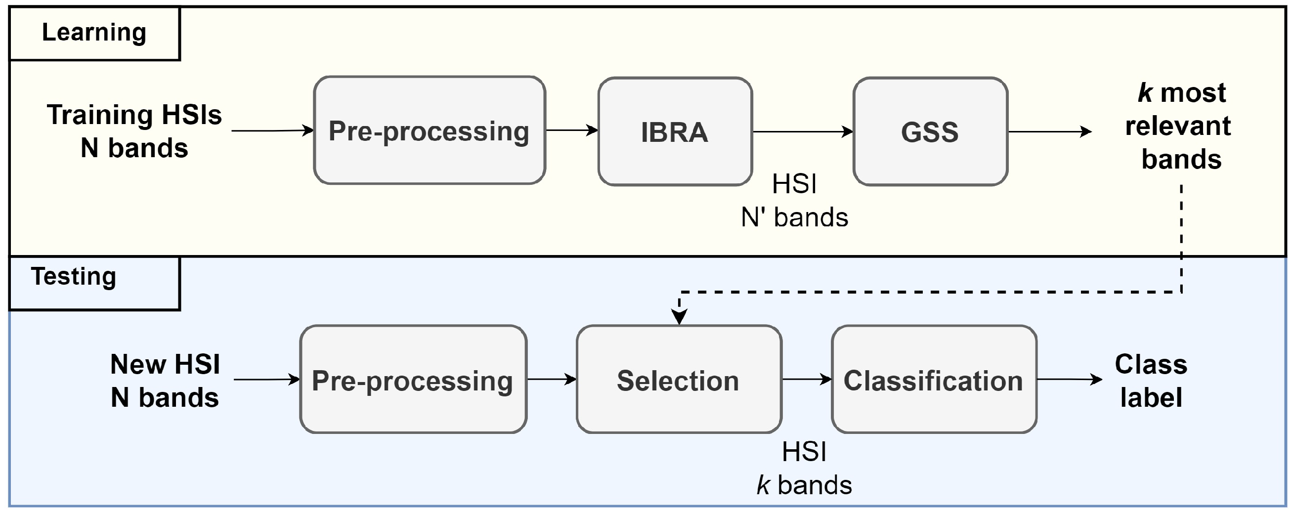
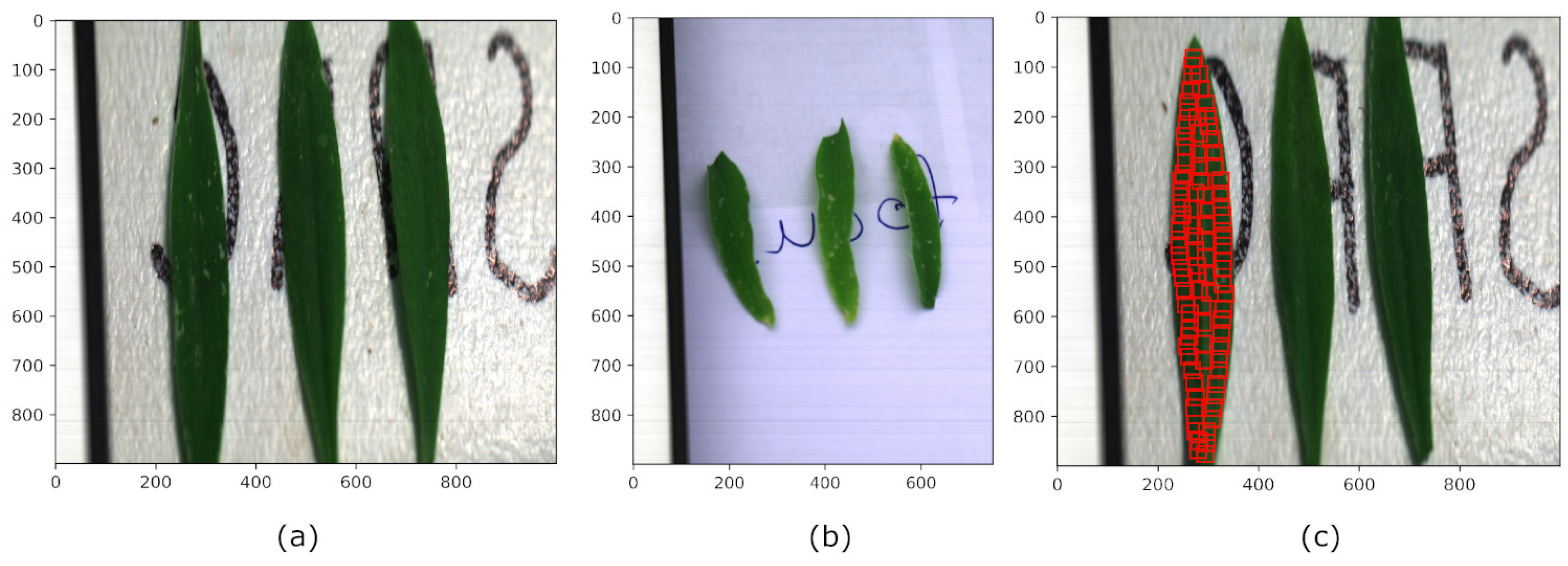
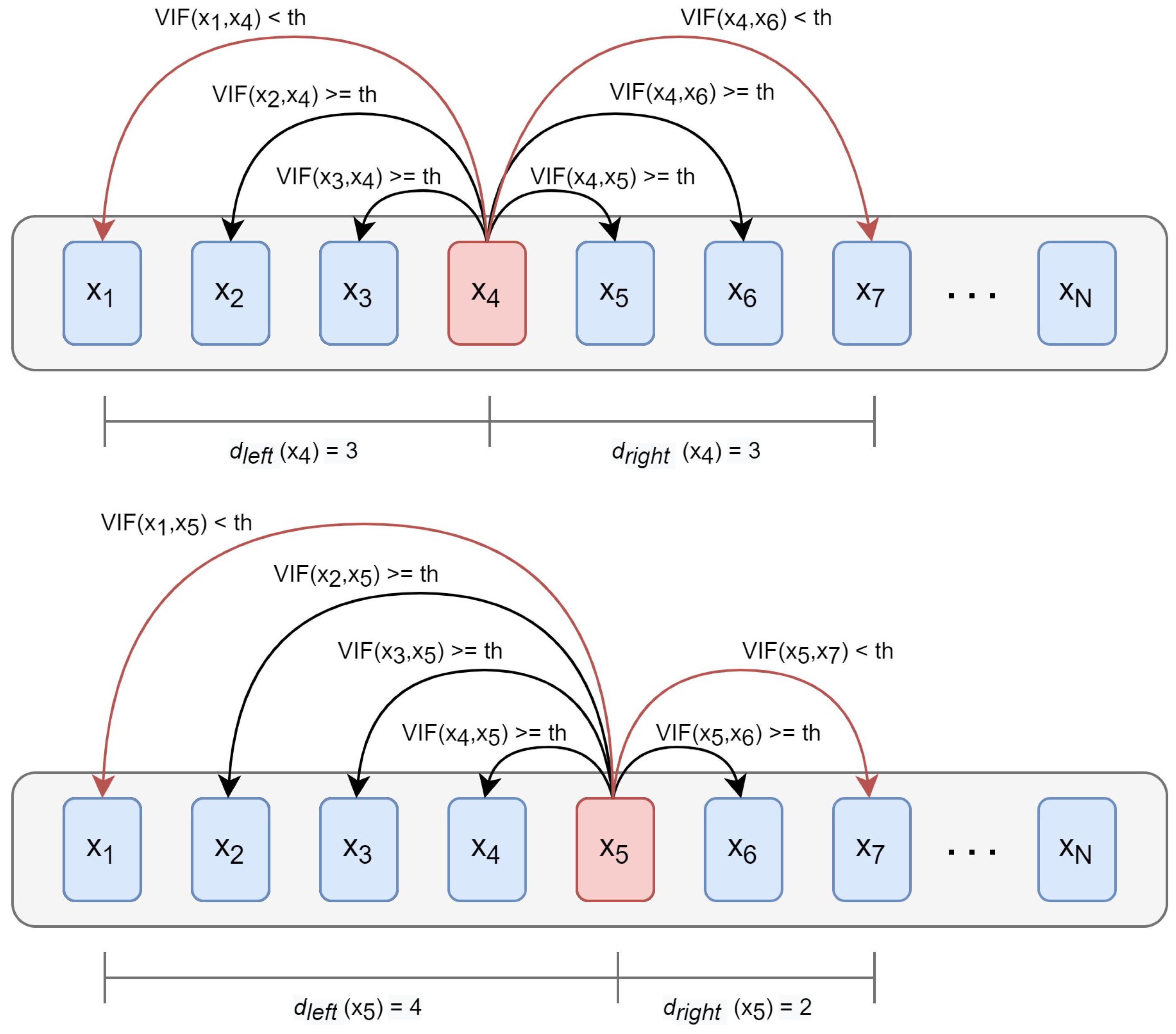
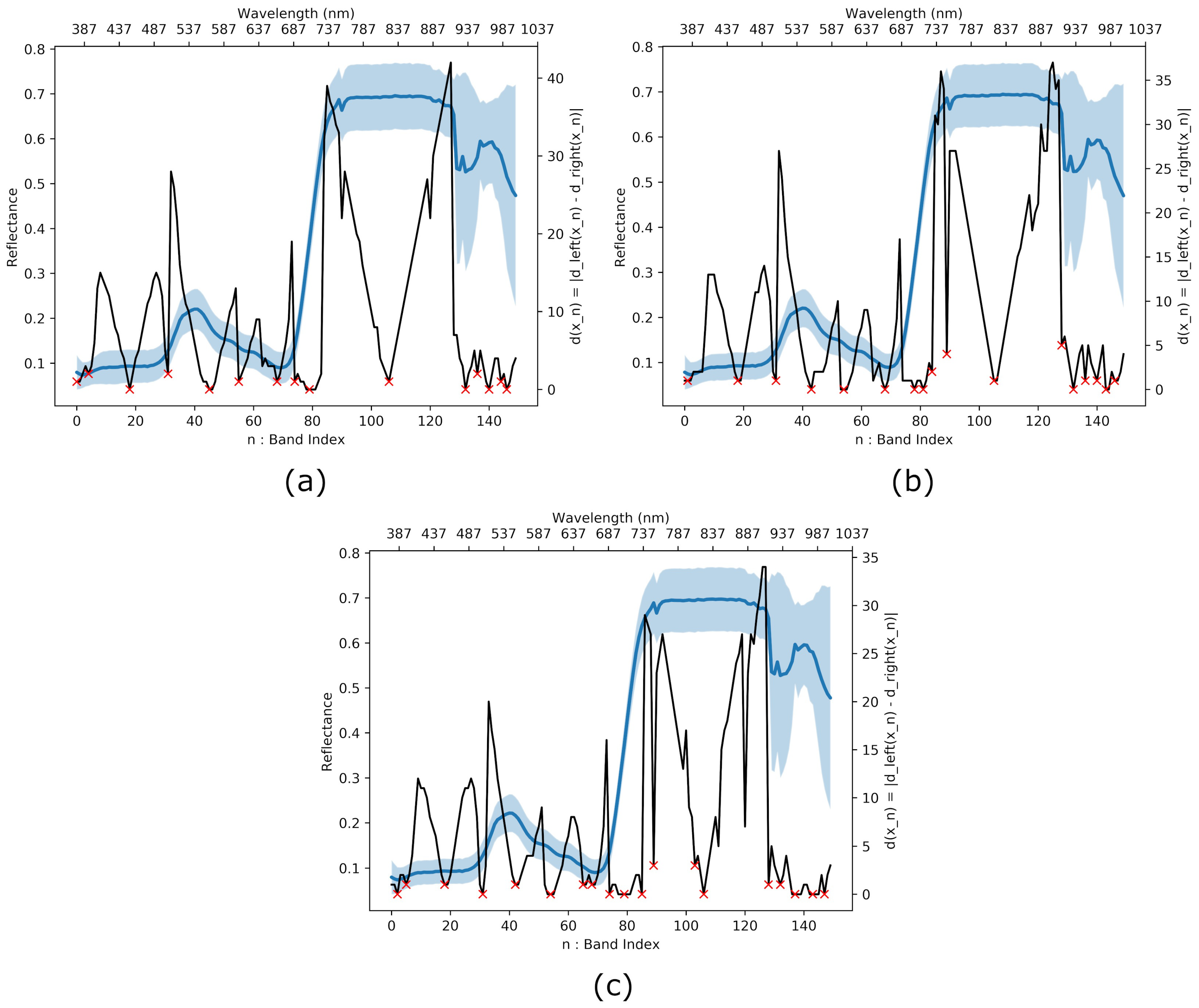
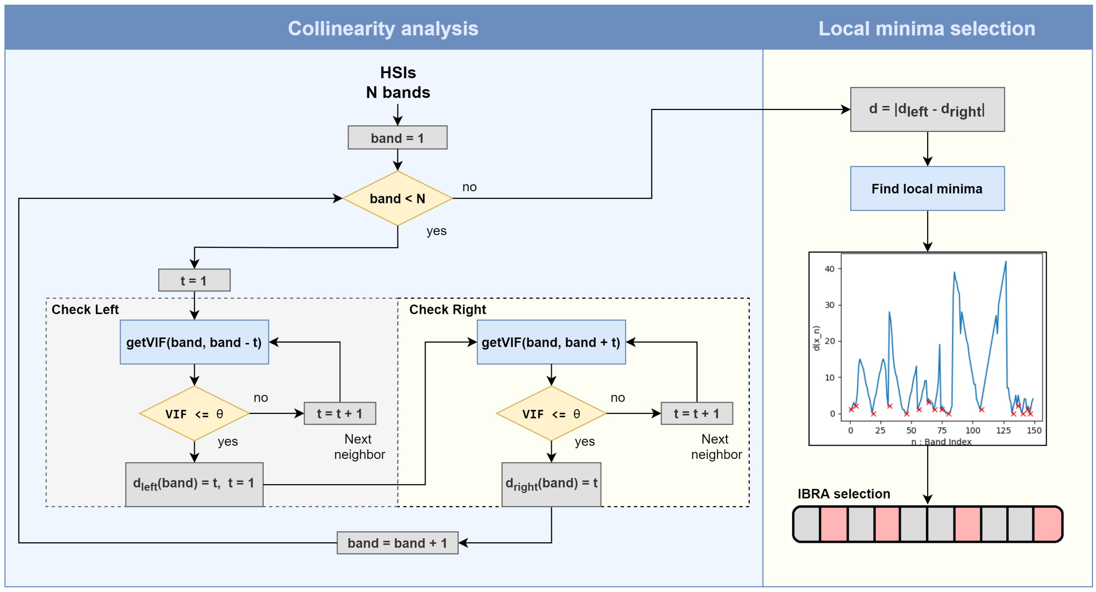
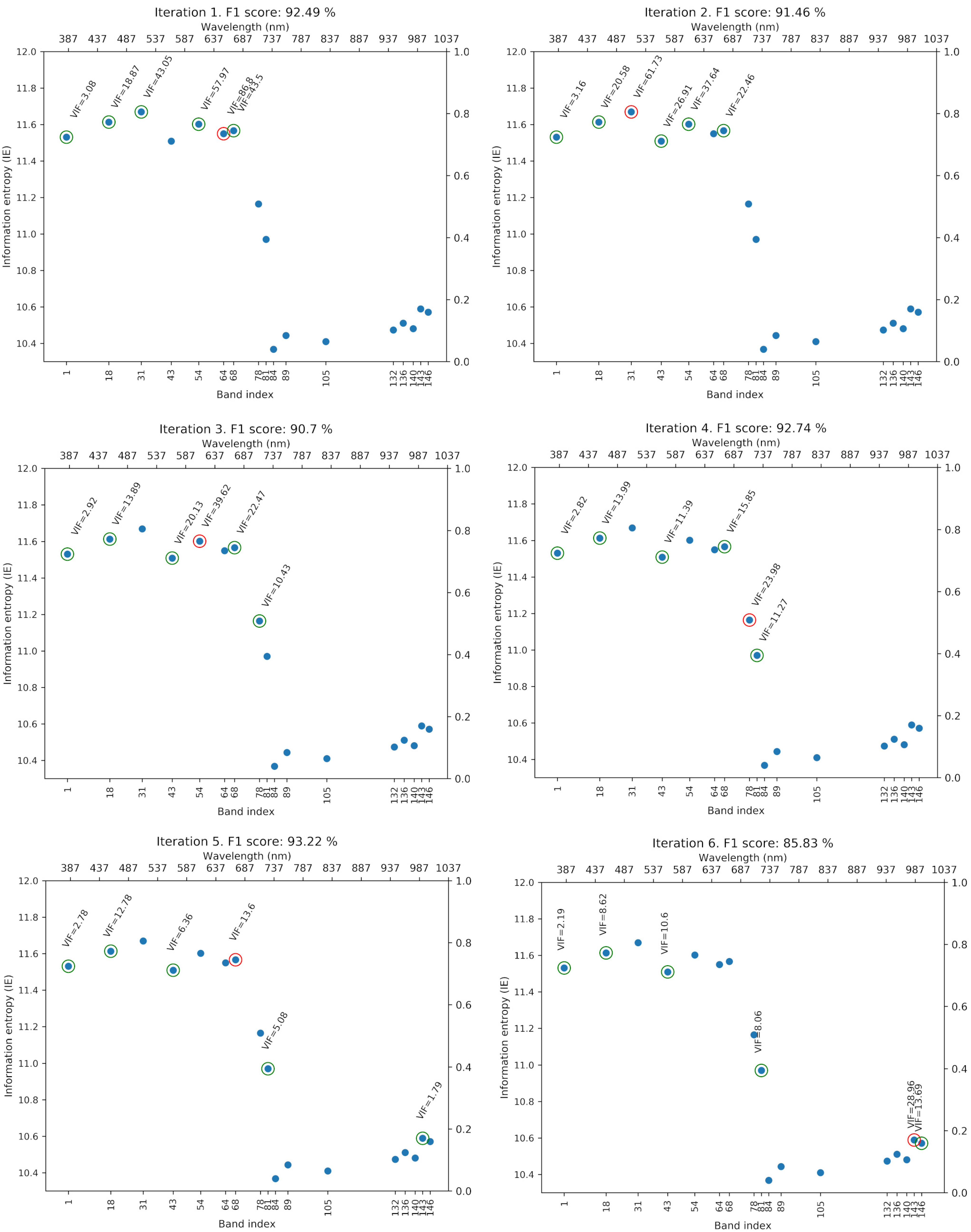
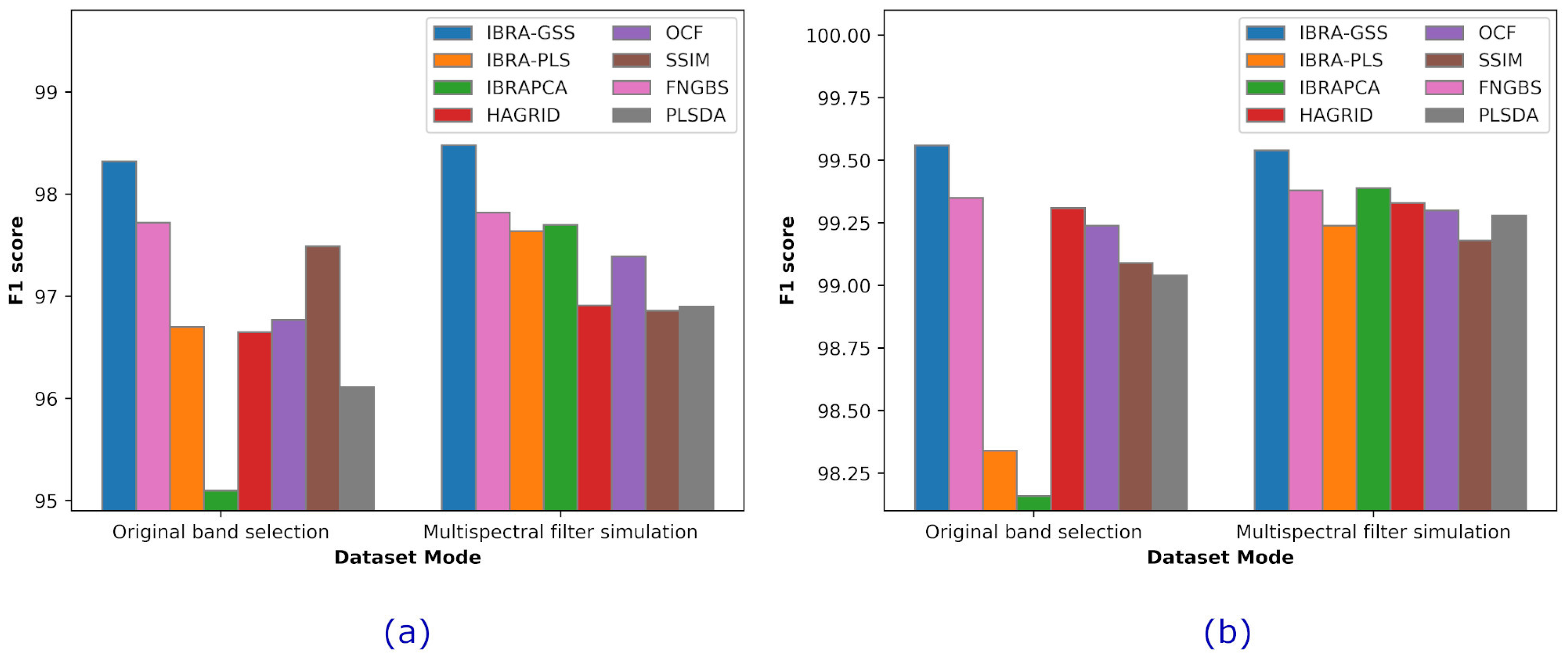
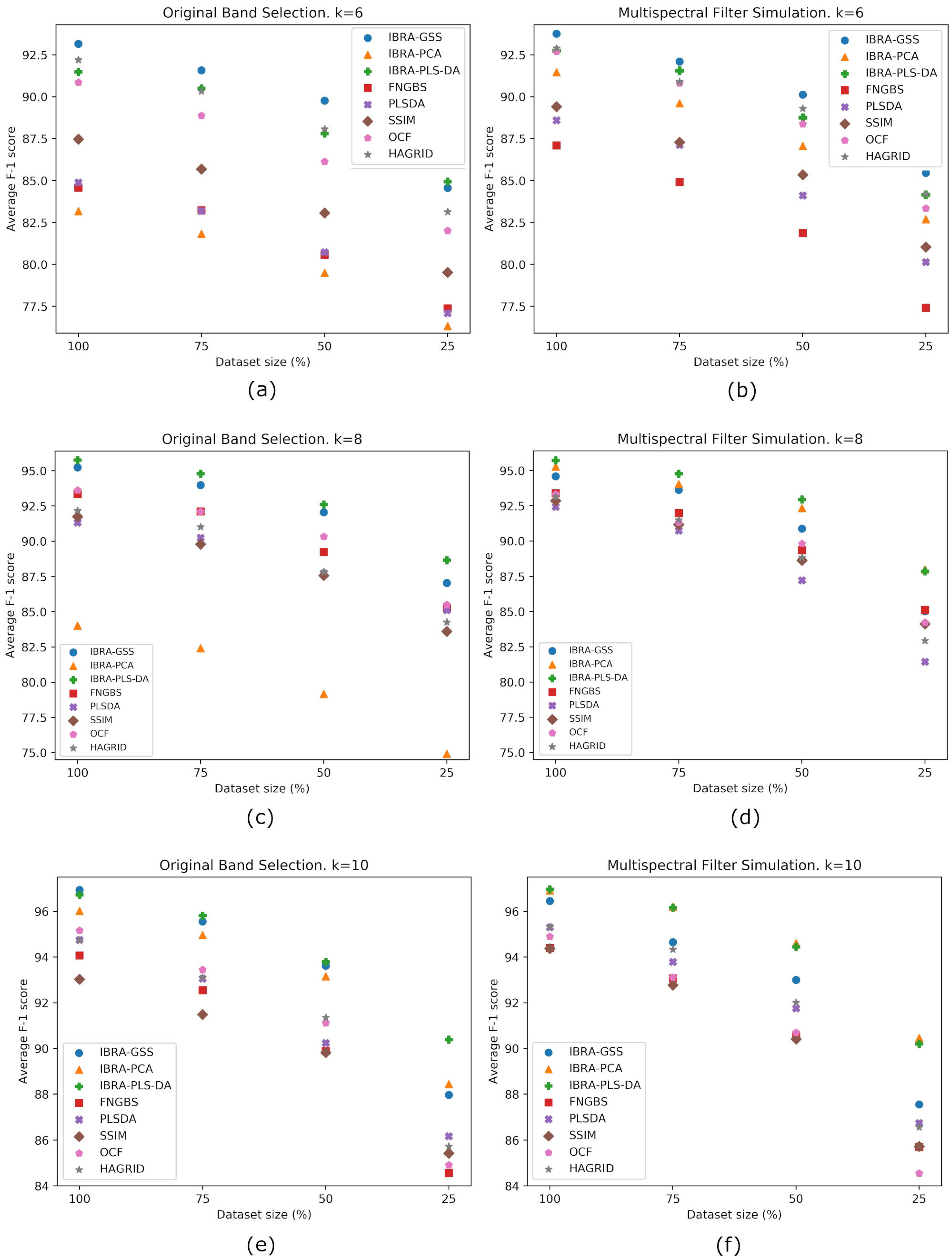
Table 1.
Hyper3DNet-Lite architecture for the Kochia dataset.
| Layer Name | Kernel Size | Stride Size | Output Size |
|---|---|---|---|
| Input | — | — | (25, 25, N, 1) |
| Conv3D + ReLU | (3, 3, 3) | (1, 1, 1) | (25, 25, N, 16) |
| Conv3D + ReLU | (3, 3, 3) | (1, 1, 1) | (25, 25, N, 16) |
| Reshape | — | — | (25, 25, ) |
| SepConv2D + ReLU | (3, 3) | (1, 1) | (25, 25, 320) |
| SepConv2D + ReLU | (3, 3) | (2, 2) | (13, 13, 256) |
| SepConv2D + ReLU | (3, 3) | (2, 2) | (7, 7, 256) |
| GlobalAveragePooling | — | — | 256 |
| Dense + Softmax | — | — | # classes |
Table 2.
Classification performance with and without IBRA preselection ().
| Dataset | # of Bands | Accuracy | Precision | Recall | F1 | # of Parameters |
|---|---|---|---|---|---|---|
| Kochia | 150 | 98.46 ± 0.29 | 98.66 ± 0.26 | 98.55 ± 0.31 | 98.60 ± 0.28 | 561,475 |
| 17 | 97.05 ± 0.47 | 97.25 ± 0.45 | 97.17 ± 0.46 | 97.21 ± 0.44 | 258,035 | |
| Indian Pines | 200 | 99.42 ± 0.18 | 99.32 ± 0.29 | 99.47 ± 0.28 | 99.39 ± 0.27 | 1,274,464 |
| 31 | 99.49 ± 0.14 | 99.38 ± 0.34 | 99.56 ± 0.19 | 99.47 ± 0.23 | 338,880 | |
| Salinas | 204 | 99.92 ± 0.04 | 99.93 ± 0.05 | 99.94 ± 0.03 | 99.94 ± 0.04 | 1,296,608 |
| 14 | 99.43 ± 0.13 | 99.75 ± 0.08 | 99.72 ± 0.08 | 99.73 ± 0.08 | 244,768 |
Table 3.
Greedy spectral selection on the Kochia dataset. Bold entries represent the best VIF threshold and average F1 score.
Table 3.
Greedy spectral selection on the Kochia dataset. Bold entries represent the best VIF threshold and average F1 score.
| k | VIF | Selected Bands (nm) | Accuracy | Precision | Recall | F1 |
|---|---|---|---|---|---|---|
| 6 | 12 | [395.5, 463.3, 565.1, 700.8, 722.0, 993.3] | 92.44 ± 0.71 | 92.76 ± 0.80 | 92.79 ± 0.67 | 92.76 ± 0.72 |
| 11 | [395.5, 408.2, 463.3, 586.3, 662.6, 700.8] | 90.74 ± 1.05 | 91.56 ± 0.97 | 91.54 ± 1.06 | 91.54 ± 1.01 | |
| 10 | [391.2, 463.3, 569.3, 675.3, 730.4, 993.3] | 92.69 ± 0.53 | 93.24 ± 0.52 | 93.08 ± 0.49 | 93.15 ± 0.49 | |
| 9 | [391.2, 463.3, 569.3, 700.8, 730.4, 993.3] | 92.40 ± 0.63 | 92.67 ± 0.63 | 92.77 ± 0.59 | 92.71 ± 0.59 | |
| 8 | [387.0, 404.0, 463.3, 577.8, 700.8, 722.0] | 92.58 ± 0.63 | 93.05 ± 0.65 | 93.08 ± 0.57 | 93.06 ± 0.59 | |
| 7 | [387.0, 404.0, 463.3, 569.3, 700.8, 722.0] | 92.07 ± 0.89 | 92.52 ± 0.89 | 92.55 ± 0.79 | 92.53 ± 0.83 | |
| 6 | [387.0, 404.0, 463.3, 586.3, 700.8, 717.7] | 92.00 ± 0.61 | 92.57 ± 0.54 | 92.52 ± 0.64 | 92.53 ± 0.57 | |
| 5 | [387.0, 463.3, 586.3, 645.6, 700.8, 722.0] | 91.03 ± 1.04 | 91.79 ± 1.14 | 91.75 ± 0.91 | 91.76 ± 1.01 | |
| 8 | 12 | [395.5, 408.2, 463.3, 565.1, 675.3, 700.8, 722.0, 993.3] | 93.96 ± 0.68 | 94.47 ± 0.65 | 94.34 ± 0.68 | 94.39 ± 0.66 |
| 11 | [395.5, 408.2, 463.3, 565.1, 675.3, 700.8, 726.2, 993.3] | 94.18 ± 0.70 | 94.74 ± 0.65 | 94.47 ± 0.67 | 94.59 ± 0.66 | |
| 10 | [391.2, 463.3, 569.3, 675.3, 730.4, 963.6, 993.3, 1006.0] | 93.95 ± 0.62 | 94.48 ± 0.56 | 94.13 ± 0.68 | 94.29 ± 0.61 | |
| 9 | [391.2, 463.3, 569.3, 671.1, 700.8, 730.4, 963.6, 993.3] | 94.33 ± 0.41 | 94.81 ± 0.48 | 94.60 ± 0.47 | 94.69 ± 0.47 | |
| 8 | [387.0, 404.0, 463.3, 518.4, 577.8, 654.1, 675.32, 700.8] | 94.79 ± 0.65 | 95.28 ± 0.55 | 95.20 ± 0.67 | 95.23 ± 0.61 | |
| 7 | [387.0, 404.0, 463.3, 569.3, 675.3, 700.8, 722.0, 1006.0] | 94.48 ± 0.77 | 95.05 ± 0.72 | 94.85 ± 0.73 | 94.93 ± 0.73 | |
| 6 | [387.0, 404.0, 463.3, 586.3, 679.6, 700.8, 730.4, 1001.8] | 94.65 ± 0.45 | 95.21 ± 0.38 | 94.89 ± 0.48 | 95.04 ± 0.42 | |
| 5 | [387.0, 463.3, 586.3, 645.6, 700.8, 722.0, 980.6, 1001.8] | 93.68 ± 0.75 | 94.25 ± 0.65 | 93.95 ± 0.68 | 94.08 ± 0.66 | |
| 10 | 12 | [395.5, 408.2, 463.3, 518.4, 565.1, 616.0, 675.3, 700.8, 722.0, 993.3] | 96.31 ± 0.69 | 96.57 ± 0.55 | 96.49 ± 0.73 | 96.53 ± 0.64 |
| 11 | [395.5, 408.2, 463.3, 565.1, 662.6, 675.3, 700.8, 713.5, 726.2, 993.3] | 96.18 ± 0.41 | 96.48 ± 0.29 | 96.31 ± 0.46 | 96.39 ± 0.36 | |
| 10 | [391.2, 463.3, 518.4, 569.3, 658.4, 675.3, 717.7, 730.4, 993.3, 1006.] | 95.83 ± 0.36 | 96.10 ± 0.38 | 96.06 ± 0.32 | 96.08 ± 0.34 | |
| 9 | [391.2, 463.3, 518.4, 569.3, 616.0, 671.1, 700.8, 717.7, 730.4, 993.3] | 96.16 ± 0.56 | 96.48 ± 0.50 | 96.37 ± 0.54 | 96.42 ± 0.52 | |
| 8 | [387.0, 404.0, 463.3, 518.4, 577.8, 654.1, 675.3, 700.8, 722.0, 1006.0] | 96.47 ± 0.38 | 96.79 ± 0.36 | 96.66 ± 0.37 | 96.72 ± 0.35 | |
| 7 | [387.0, 404.0, 463.3, 518.4, 569.3, 654.1, 675.3, 700.8, 722.0, 1006.0] | 96.69 ± 0.35 | 96.92 ± 0.38 | 96.95 ± 0.34 | 96.93 ± 0.35 | |
| 6 | [387.0, 404.0, 463.3, 586.3, 649.9, 679.6, 700.8, 717.7, 730.4, 1001.8] | 95.91 ± 0.50 | 96.34 ± 0.44 | 96.12 ± 0.47 | 96.22 ± 0.45 | |
| 5 | [387.0, 463.3, 586.3, 645.6, 700.8, 722.0, 832.2, 946.7, 980.6, 1001.8] | 95.06 ± 0.54 | 95.44 ± 0.52 | 95.33 ± 0.56 | 95.38 ± 0.53 |
Table 4.
Greedy spectral selection on the IP dataset. Bold entries represent the best VIF threshold and average F1 score.
Table 4.
Greedy spectral selection on the IP dataset. Bold entries represent the best VIF threshold and average F1 score.
| VIF | Selected Bands (nm) | Accuracy | Precision | Recall | F1 |
|---|---|---|---|---|---|
| 12 | [498.3, 646.7, 706.2, 754.4, 1023.7] | 97.96 ± 0.33 | 98.21 ± 0.43 | 98.32 ± 0.33 | 98.25 ± 0.35 |
| 11 | [557.5, 587.2, 706.2, 754.4, 1023.7] | 97.55 ± 0.29 | 98.05 ± 0.29 | 97.95 ± 0.29 | 97.98 ± 0.22 |
| 10 | [498.3, 626.9, 706.2, 754.4, 1023.7] | 98.08 ± 0.43 | 98.26 ± 0.42 | 98.39 ± 0.43 | 98.32 ± 0.39 |
| 9 | [557.5, 626.9, 706.2, 821.8, 1023.7] | 98.28 ± 0.35 | 98.24 ± 0.47 | 98.06 ± 0.59 | 98.11 ± 0.43 |
| 8 | [607.0, 646.7, 706.2, 821.8, 1023.7] | 98.04 ± 0.30 | 98.19 ± 0.46 | 98.06 ± 0.46 | 98.10 ± 0.35 |
| 7 | [567.4, 587.2, 706.2, 821.8, 1023.7] | 98.01 ± 0.24 | 98.29 ± 0.18 | 98.36 ± 0.42 | 98.31 ± 0.26 |
| 6 | [577.3, 706.2, 821.8, 918.0, 1023.7] | 97.06 ± 0.49 | 97.49 ± 0.58 | 97.63 ± 0.48 | 97.53 ± 0.48 |
| 5 | [577.3, 715.8, 812.2, 918.0, 1023.7] | 96.73 ± 0.55 | 97.46 ± 0.53 | 97.00 ± 0.61 | 97.19 ± 0.49 |
Table 5.
Greedy spectral selection on the SA dataset. Bold entries represent the best VIF threshold and average F1 score.
Table 5.
Greedy spectral selection on the SA dataset. Bold entries represent the best VIF threshold and average F1 score.
| VIF | Selected Bands (nm) | Accuracy | Precision | Recall | F1 |
|---|---|---|---|---|---|
| 12 | [532.1, 731.8, 950.5, 1368.9, 2224.7] | 98.70 ± 0.11 | 99.40 ± 0.05 | 99.48 ± 0.04 | 99.44 ± 0.04 |
| 11 | [541.7, 731.8, 950.5, 1368.9, 2224.7] | 98.68 ± 0.11 | 99.36 ± 0.10 | 99.45 ± 0.05 | 99.40 ± 0.07 |
| 10 | [541.7, 731.8, 950.5, 1359.4, 2224.7] | 98.62 ± 0.14 | 99.38 ± 0.07 | 99.45 ± 0.04 | 99.41 ± 0.05 |
| 9 | [541.7, 731.8, 950.5, 1359.4, 2224.7] | 98.62 ± 0.14 | 99.38 ± 0.07 | 99.45 ± 0.04 | 99.41 ± 0.05 |
| 8 | [731.8, 950.5, 1159.7, 1254.8, 2224.7] | 99.05 ± 0.05 | 99.56 ± 0.04 | 99.55 ± 0.03 | 99.56 ± 0.03 |
| 7 | [731.8, 950.5, 1159.7, 1254.8, 2215.2] | 99.02 ± 0.10 | 99.54 ± 0.07 | 99.53 ± 0.06 | 99.54 ± 0.06 |
| 6 | [570.2, 950.5, 1245.3, 1368.9, 2215.2] | 99.02 ± 0.05 | 99.54 ± 0.04 | 99.56 ± 0.02 | 99.55 ± 0.03 |
| 5 | [560.7, 950.5, 1245.3, 1368.9, 2215.2] | 98.99 ± 0.06 | 99.52 ± 0.09 | 99.56 ± 0.05 | 99.54 ± 0.07 |
Table 6.
Dimensionality reduction method comparison—Kochia dataset. Bold entries represent the best classification scores for each k.
Table 6.
Dimensionality reduction method comparison—Kochia dataset. Bold entries represent the best classification scores for each k.
| k | Method | Accuracy | Precision | Recall | F1 |
|---|---|---|---|---|---|
| 6 | FNGBS | 84.32 ± 1.78 | 84.85 ± 1.77 | 84.37 ± 1.72 | 84.59 ± 1.73 |
| 86.98 ± 0.84 | 87.35 ± 0.80 | 86.91 ± 0.91 | 87.10 ± 0.83 | ||
| PLS-DA | 84.77 ± 1.83 | 85.15 ± 1.89 | 84.69 ± 1.82 | 84.89 ± 1.82 | |
| 88.41 ± 0.79 | 88.85 ± 0.62 | 88.37 ± 0.96 | 88.59 ± 0.78 | ||
| SR-SSIM | 86.42 ± 1.07 | 87.66 ± 1.02 | 87.31 ± 1.06 | 87.47 ± 1.03 | |
| 88.73 ± 0.90 | 89.55 ± 0.81 | 89.30 ± 0.99 | 89.41 ± 0.89 | ||
| OCF | 90.48 ± 0.57 | 90.92 ± 0.62 | 90.81 ± 0.44 | 90.86 ± 0.49 | |
| 92.42 ± 0.67 | 92.75 ± 0.66 | 92.66 ± 0.66 | 92.70 ± 0.65 | ||
| HAGRID | 91.71 ± 0.83 | 92.25 ± 0.78 | 92.17 ± 0.84 | 92.20 ± 0.80 | |
| 92.48 ± 0.62 | 92.91 ± 0.53 | 92.89 ± 0.58 | 92.89 ± 0.54 | ||
| IBRA-PCA | 83.04 ± 2.23 | 83.44 ± 2.16 | 82.96 ± 2.40 | 83.17 ± 2.29 | |
| 91.31 ± 0.74 | 91.81 ± 0.67 | 91.18 ± 0.71 | 91.46 ± 0.68 | ||
| IBRA-PLS-DA | 90.81 ± 0.96 | 91.68 ± 1.04 | 91.33 ± 0.86 | 91.48 ± 0.94 | |
| 92.29 ± 0.63 | 92.98 ± 0.58 | 92.57 ± 0.72 | 92.76 ± 0.65 | ||
| IBRA-GSS | 92.69 ± 0.53 | 93.24 ± 0.52 | 93.08 ± 0.50 | 93.15 ± 0.49 | |
| 93.32 ± 0.68 | 93.80 ± 0.64 | 93.74 ± 0.66 | 93.76 ± 0.64 | ||
| 8 | FNGBS | 92.88 ± 0.55 | 93.63 ± 0.55 | 93.10 ± 0.46 | 93.34 ± 0.50 |
| 93.12 ± 0.32 | 93.69 ± 0.28 | 93.13 ± 0.46 | 93.39 ± 0.34 | ||
| PLS-DA | 90.53 ± 1.65 | 91.70 ± 1.37 | 91.01 ± 1.72 | 91.32 ± 1.57 | |
| 91.92 ± 0.81 | 92.69 ± 0.71 | 92.21 ± 0.87 | 92.43 ± 0.79 | ||
| SR-SSIM | 91.01 ± 1.37 | 91.97 ± 1.28 | 91.54 ± 1.35 | 91.75 ± 1.31 | |
| 92.31 ± 0.83 | 93.00 ± 0.81 | 92.73 ± 0.89 | 92.86 ± 0.83 | ||
| OCF | 93.05 ± 0.90 | 93.86 ± 0.80 | 93.43 ± 0.84 | 93.62 ± 0.83 | |
| 92.89 ± 0.71 | 93.45 ± 0.64 | 93.21 ± 0.67 | 93.32 ± 0.65 | ||
| HAGRID | 91.59 ± 1.25 | 92.52 ± 1.05 | 91.88 ± 1.24 | 92.17 ± 1.16 | |
| 92.82 ± 0.79 | 93.41 ± 0.69 | 92.92 ± 0.91 | 93.15 ± 0.80 | ||
| IBRA-PCA | 83.75 ± 2.40 | 84.33 ± 2.48 | 83.77 ± 2.43 | 84.02 ± 2.45 | |
| 95.04 ± 0.70 | 95.35 ± 0.60 | 95.21 ± 0.81 | 95.27 ± 0.70 | ||
| IBRA-PLS-DA | 95.46 ± 0.53 | 95.91 ± 0.46 | 95.63 ± 0.49 | 95.76 ± 0.47 | |
| 95.42 ± 0.60 | 95.85 ± 0.52 | 95.62 ± 0.57 | 95.72 ± 0.53 | ||
| IBRA-GSS | 94.79 ± 0.65 | 95.28 ± 0.55 | 95.20 ± 0.67 | 95.23 ± 0.61 | |
| 94.08 ± 0.60 | 94.67 ± 0.57 | 94.54 ± 0.54 | 94.60 ± 0.54 | ||
| 10 | FNGBS | 93.78 ± 0.77 | 94.17 ± 0.84 | 93.99 ± 0.73 | 94.08 ± 0.78 |
| 94.19 ± 0.47 | 94.54 ± 0.47 | 94.27 ± 0.51 | 94.39 ± 0.48 | ||
| PLS-DA | 94.36 ± 0.51 | 94.86 ± 0.55 | 94.67 ± 0.47 | 94.76 ± 0.49 | |
| 95.10 ± 0.68 | 95.44 ± 0.59 | 95.18 ± 0.67 | 95.30 ± 0.63 | ||
| OCF | 94.87 ± 0.51 | 95.23 ± 0.52 | 95.11 ± 0.46 | 95.16 ± 0.47 | |
| 94.62 ± 0.73 | 95.00 ± 0.65 | 94.80 ± 0.64 | 94.89 ± 0.64 | ||
| SR-SSIM | 93.84 ± 0.62 | 94.50 ± 0.57 | 94.27 ± 0.64 | 94.37 ± 0.59 | |
| 94.36 ± 0.51 | 94.86 ± 0.55 | 94.67 ± 0.47 | 94.76 ± 0.50 | ||
| HAGRID | 94.50 ± 0.81 | 94.81 ± 0.78 | 94.69 ± 0.72 | 94.74 ± 0.74 | |
| 95.14 ± 0.51 | 95.49 ± 0.48 | 95.18 ± 0.51 | 95.33 ± 0.47 | ||
| IBRA-PCA | 95.69 ± 0.44 | 96.13 ± 0.44 | 95.92 ± 0.38 | 96.02 ± 0.39 | |
| 96.74 ± 0.30 | 96.96 ± 0.29 | 96.85 ± 0.28 | 96.91 ± 0.27 | ||
| IBRA-PLS-DA | 96.51 ± 0.46 | 96.78 ± 0.43 | 96.67 ± 0.44 | 96.72 ± 0.42 | |
| 96.82 ± 0.50 | 97.08 ± 0.44 | 96.86 ± 0.54 | 96.97 ± 0.48 | ||
| IBRA-GSS | 96.69 ± 0.35 | 96.92 ± 0.38 | 96.95 ± 0.34 | 96.93 ± 0.35 | |
| 96.21 ± 0.49 | 96.51 ± 0.45 | 96.40 ± 0.44 | 96.45 ± 0.44 |
Table 7.
Dimensionality reduction method comparison—Indian Pines dataset, . Bold entries represent the best classification scores.
Table 7.
Dimensionality reduction method comparison—Indian Pines dataset, . Bold entries represent the best classification scores.
| Method | Accuracy | Precision | Recall | F1 |
|---|---|---|---|---|
| PLS-DA | 96.68 ± 0.86 | 96.83 ± 0.99 | 95.62 ± 0.94 | 96.11 ± 0.74 |
| 97.17 ± 0.60 | 97.30 ± 0.79 | 96.66 ± 1.03 | 96.90 ± 0.84 | |
| OCF | 96.68 ± 0.56 | 97.34 ± 0.76 | 96.34 ± 0.98 | 96.77 ± 0.82 |
| 97.02 ± 0.58 | 97.73 ± 0.51 | 97.14 ± 0.63 | 97.39 ± 0.48 | |
| HAGRID | 96.74 ± 0.54 | 97.06 ± 0.75 | 96.34 ± 1.03 | 96.65 ± 0.88 |
| 97.03 ± 0.75 | 97.24 ± 0.86 | 96.72 ± 1.45 | 96.91 ± 1.21 | |
| SR-SSIM | 97.28 ± 0.37 | 97.74 ± 0.44 | 97.34 ± 0.80 | 97.49 ± 0.57 |
| 96.83 ± 0.77 | 97.14 ± 1.02 | 96.82 ± 1.95 | 96.86 ± 1.47 | |
| FNGBS | 97.49 ± 0.34 | 97.86 ± 0.36 | 97.64 ± 0.71 | 97.72 ± 0.5 |
| 97.34 ± 0.65 | 97.94 ± 0.52 | 97.75 ± 0.46 | 97.82 ± 0.44 | |
| IBRA-PCA | 94.70 ± 0.65 | 96.12 ± 0.71 | 94.45 ± 1.52 | 95.10 ± 1.02 |
| 96.99 ± 0.97 | 97.84 ± 0.77 | 97.60 ± 0.39 | 97.70 ± 0.55 | |
| IBRA-PLS-DA | 96.11 ± 1.37 | 97.10 ± 1.04 | 96.60 ± 0.98 | 96.70 ± 1.01 |
| 97.19 ± 0.67 | 97.77 ± 0.67 | 97.67 ± 1.03 | 97.64 ± 0.95 | |
| IBRA-GSS | 98.08 ± 0.43 | 98.26 ± 0.42 | 98.39 ± 0.43 | 98.32 ± 0.39 |
| 98.24 ± 0.39 | 98.56 ± 0.38 | 98.43 ± 0.42 | 98.48 ± 0.36 |
Table 8.
Dimensionality reduction method comparison—Salinas dataset, . Bold entries represent the best classification scores.
Table 8.
Dimensionality reduction method comparison—Salinas dataset, . Bold entries represent the best classification scores.
| Method | Accuracy | Precision | Recall | F1 |
|---|---|---|---|---|
| PLS-DA | 97.89 ± 0.18 | 98.99 ± 0.09 | 99.10 ± 0.10 | 99.04 ± 0.09 |
| 98.46 ± 0.10 | 99.24 ± 0.04 | 99.33 ± 0.03 | 99.28 ± 0.03 | |
| OCF | 98.37 ± 0.14 | 99.20 ± 0.07 | 99.29 ± 0.07 | 99.24 ± 0.07 |
| 98.51 ± 0.12 | 99.27 ± 0.08 | 99.34 ± 0.06 | 99.30 ± 0.07 | |
| HAGRID | 98.47 ± 0.11 | 99.26 ± 0.09 | 99.36 ± 0.05 | 99.31 ± 0.06 |
| 98.51 ± 0.12 | 99.29 ± 0.08 | 99.37 ± 0.05 | 99.33 ± 0.06 | |
| SR-SSIM | 97.89 ± 0.22 | 99.11 ± 0.11 | 99.07 ± 0.09 | 99.09 ± 0.09 |
| 98.14 ± 0.21 | 99.18 ± 0.12 | 99.18 ± 0.09 | 99.18 ± 0.10 | |
| FNGBS | 98.44 ± 0.14 | 99.34 ± 0.08 | 99.37 ± 0.06 | 99.35 ± 0.07 |
| 98.51 ± 0.10 | 99.37 ± 0.05 | 99.39 ± 0.04 | 99.38 ± 0.04 | |
| IBRA-PCA | 96.10 ± 0.78 | 98.23 ± 0.34 | 98.14 ± 0.49 | 98.16 ± 0.45 |
| 98.49 ± 0.16 | 99.39 ± 0.07 | 99.39 ± 0.07 | 99.39 ± 0.06 | |
| IBRA-PLS-DA | 96.26 ± 0.21 | 98.33 ± 0.14 | 98.36 ± 0.11 | 98.34 ± 0.10 |
| 98.14 ± 0.20 | 99.25 ± 0.08 | 99.23 ± 0.09 | 99.24 ± 0.08 | |
| IBRA-GSS | 99.05 ± 0.05 | 99.56 ± 0.04 | 99.55 ± 0.03 | 99.56 ± 0.03 |
| 99.07 ± 0.09 | 99.53 ± 0.06 | 99.55 ± 0.03 | 99.54 ± 0.04 |
Table 9.
Statistical significance tests—Kochia dataset. p-values obtained comparing the classification performance of IBRA-GSS to that of the other six dimensionality reduction methods.
Table 9.
Statistical significance tests—Kochia dataset. p-values obtained comparing the classification performance of IBRA-GSS to that of the other six dimensionality reduction methods.
| Compared Method | Kochia, | Kochia, | Kochia, | |||
|---|---|---|---|---|---|---|
| t-Test | Perm. | t-Test | Perm. | t-Test | Perm. | |
| FNGBS | 7.4 × (↑) | 2 × (↑) | 4.2 × (↑) | 1.7 × (↑) | 1 × (↑) | 2 × (↑) |
| 1.8 × (↑) | 2 × (↑) | 5.9 × (↑) | 1.7 × (↑) | 3.7 × (↑) | 2 × (↑) | |
| PLS-DA | 6.5 × (↑) | 2.6 × (↑) | 2.1 × (↑) | 2.6 × (↑) | 1.4 × (↑) | 2.6 × (↑) |
| 1.2 × (↑) | 2.6 × (↑) | 3.9 × (↑) | 2.6 × (↑) | 3.6 × (↑) | 2.6 × (↑) | |
| SR-SSIM | 1 × (↑) | 2 × (↑) | 2.6 × (↑) | 2 × (↑) | 9.9 × (↑) | 2 × (↑) |
| 1 × (↑) | 2 × (↑) | 4.2 × (↑) | 2 × (↑) | 9.9 × (↑) | 2 × (↑) | |
| OCF | 3 × (↑) | 1.9 × (↑) | 6.3 × (↑) | 3.5 × (↑) | 8 × (↑) | 1.9 × (↑) |
| 2 × (↑) | 5.4 × (↑) | 1.2 × (↑) | 1.9 × (↑) | 1.2 × (↑) | 1.9 × (↑) | |
| HAGRID | 9.1 × (↑) | 1.6 × (↑) | 5.3 × (↑) | 1.6 × (↑) | 2.1 × (↑) | 1.6 × (↑) |
| 2.8 × (↑) | 3.3 × (↑) | 5.5 × (↑) | 1.6 × (↑) | 1.6 × (↑) | 1.6 × (↑) | |
| IBRA-PCA | 3.8 × (↑) | 1.8 × (↑) | 1.9 × (↑) | 1.8 × (↑) | 9 × (↑) | 1.8 × (↑) |
| 2.9 × (↑) | 1.8 × (↑) | 1.6 (↓) | 2.3 (↓) | 5.6 (=) | 5.9 × (=) | |
| IBRA-PLS-DA | 1.8 × (↑) | 1.7 × (↑) | 2.1 (↓) | 1.2 (↓) | 0.18 (=) | 0.18 (=) |
| 7 × (↑) | 0.012 (↑) | 5.1 (↓) | 1.7 (↓) | 1.3 (↓) | 1.9 (↓) | |
Table 10.
Statistical significance tests—Indian Pines and Salinas datasets. p-values obtained comparing the classification performance of IBRA-GSS to that of the other six dimensionality reduction methods.
Table 10.
Statistical significance tests—Indian Pines and Salinas datasets. p-values obtained comparing the classification performance of IBRA-GSS to that of the other six dimensionality reduction methods.
| Compared Method | IP, | SA, | ||
|---|---|---|---|---|
| t-Test | Perm. | t-Test | Perm. | |
| FNGBS | 1 × (↑) | 5.7 × (↑) | 4.1 × (↑) | 2 × (↑) |
| 1.2 × (↑) | 0.014 (↑) | 2.8 × (↑) | 1.7 × (↑) | |
| PLS-DA | 1 × (↑) | 2.6 × (↑) | 3.4 × (↑) | 2.6 × (↑) |
| 5.2 × (↑) | 2.6 × (↑) | 1.4 × (↑) | 1.8 × (↑) | |
| SR-SSIM | 2.5 × (↑) | 3.6 × (↑) | 1.9 × (↑) | 2 × (↑) |
| 2.5 × (↑) | 3.6 × (↑) | 1.9 × (↑) | 2 × (↑) | |
| OCF | 3 × (↑) | 1.9 × (↑) | 3.3 × (↑) | 1.9 × (↑) |
| 4.7 × (↑) | 1.9 × (↑) | 4.2 × (↑) | 1.6 × (↑) | |
| HAGRID | 3 × (↑) | 1.6 × (↑) | 2.8 × (↑) | 1.6 × (↑) |
| 2.5 × (↑) | 3.4 × (↑) | 3.6 × (↑) | 1.9 × (↑) | |
| IBRA-PCA | 7.9 × (↑) | 1.8 × (↑) | 5.4 × (↑) | 1.8 × (↑) |
| 1 × (↑) | 1.8 × (↑) | 5.3 × (↑) | 2.6 × (↑) | |
| IBRA-PLS-DA | 2.7 × (↑) | 1.7 × (↑) | 2.9 × (↑) | 1.7 × (↑) |
| 2.5 × (↑) | 1.3 × (↑) | 1.4 × (↑) | 1.7 × (↑) | |
Table 11.
Dispersion analysis of the F1 scores obtained using all the compared dimensionality reduction methods on the full Kochia dataset.
Table 11.
Dispersion analysis of the F1 scores obtained using all the compared dimensionality reduction methods on the full Kochia dataset.
| # Bands | ||||
|---|---|---|---|---|
| Metric | ||||
| Mean | 88.48 | 92.15 | 95.18 | |
| 91.08 | 93.84 | 95.58 | ||
| Std | 3.93 | 3.68 | 1.43 | |
| 2.38 | 1.31 | 1.13 | ||
| F statistic | 75.99 | 69.29 | 34.05 | |
| 102.65 | 29.1 | 38.98 | ||
| p-value | 1.1 × | 1.9 × | 2 × | |
| 7.2 × | 1.3 × | 4.8 × | ||
Publisher’s Note: MDPI stays neutral with regard to jurisdictional claims in published maps and institutional affiliations. |
© 2021 by the authors. Licensee MDPI, Basel, Switzerland. This article is an open access article distributed under the terms and conditions of the Creative Commons Attribution (CC BY) license (https://creativecommons.org/licenses/by/4.0/).
Share and Cite
MDPI and ACS Style
Morales, G.; Sheppard, J.W.; Logan, R.D.; Shaw, J.A. Hyperspectral Dimensionality Reduction Based on Inter-Band Redundancy Analysis and Greedy Spectral Selection. Remote Sens. 2021, 13, 3649. https://doi.org/10.3390/rs13183649
AMA Style
Morales G, Sheppard JW, Logan RD, Shaw JA. Hyperspectral Dimensionality Reduction Based on Inter-Band Redundancy Analysis and Greedy Spectral Selection. Remote Sensing. 2021; 13(18):3649. https://doi.org/10.3390/rs13183649
Chicago/Turabian StyleMorales, Giorgio, John W. Sheppard, Riley D. Logan, and Joseph A. Shaw. 2021. "Hyperspectral Dimensionality Reduction Based on Inter-Band Redundancy Analysis and Greedy Spectral Selection" Remote Sensing 13, no. 18: 3649. https://doi.org/10.3390/rs13183649
Note that from the first issue of 2016, this journal uses article numbers instead of page numbers. See further details here.