
A First Approach to Determine If It Is Possible to Delineate In-Season N Fertilization Maps for Wheat Using NDVI Derived from Sentinel-2


Abstract
:
1. Introduction
2. Materials and Methods
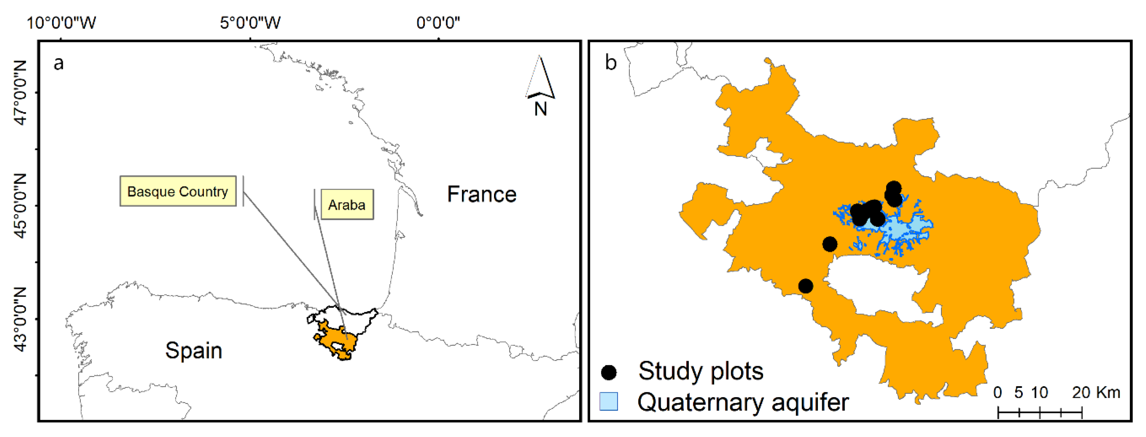
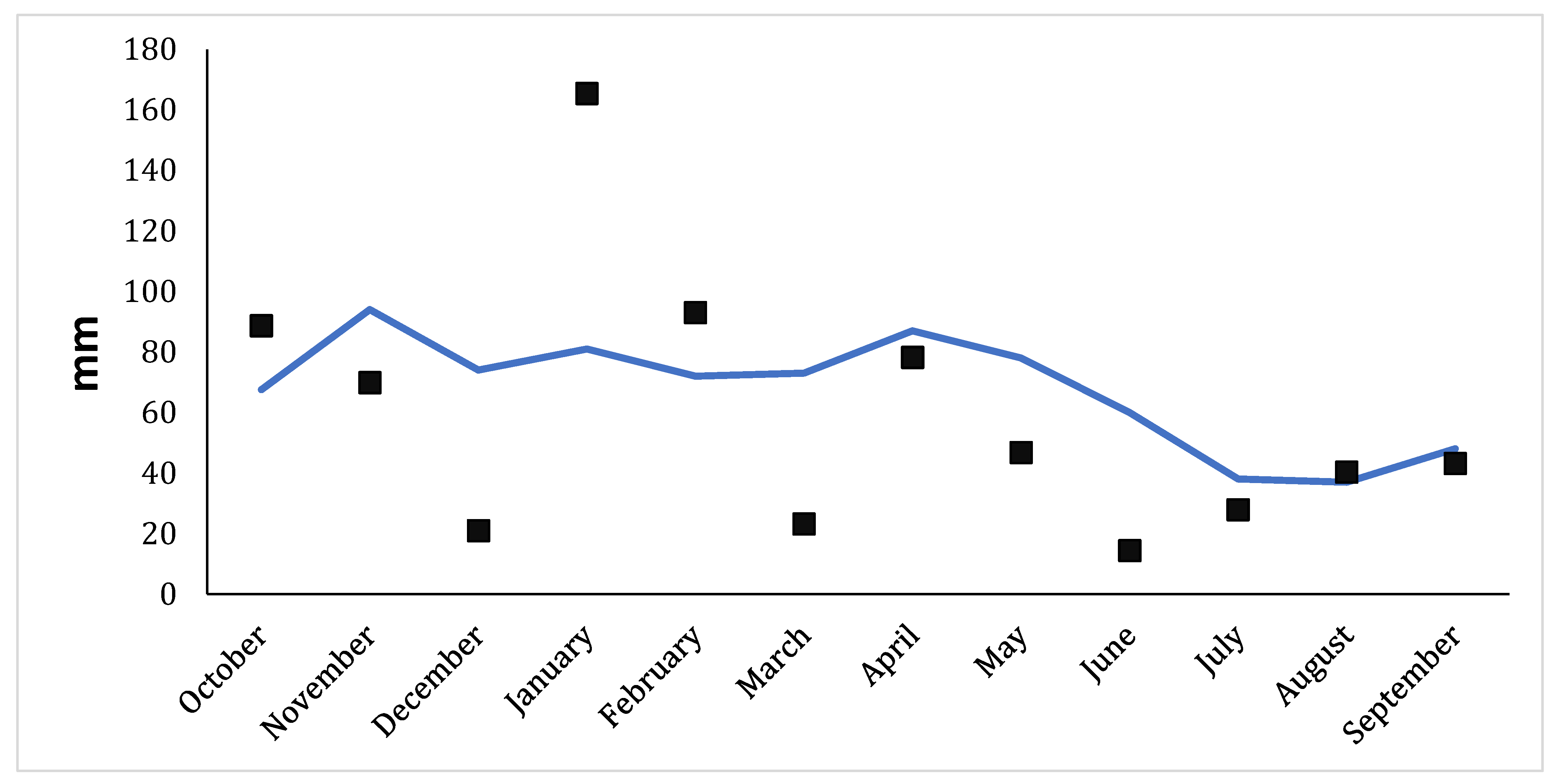
2.1. Study Area
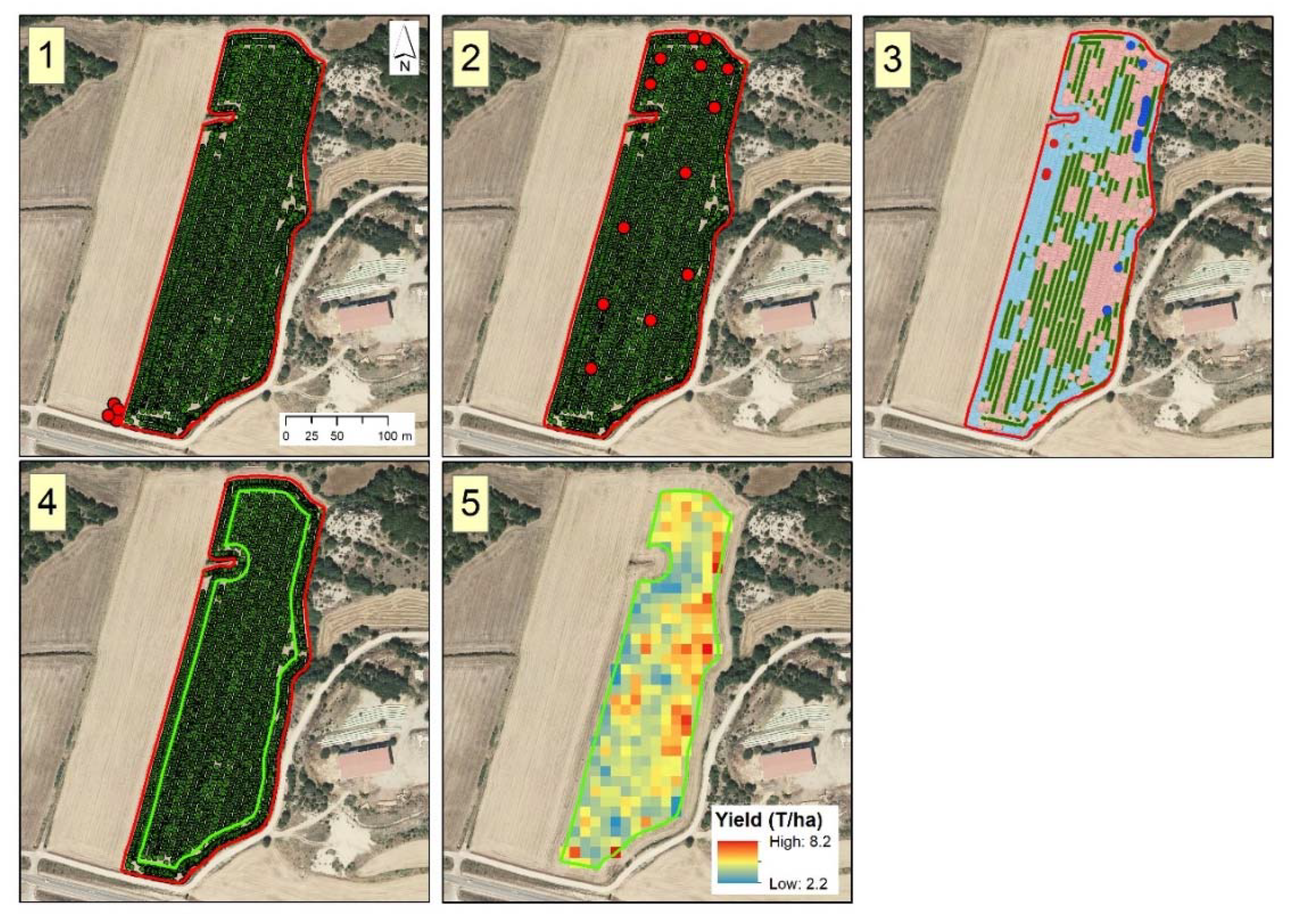
2.2. Yield Data
2.3. Sentinel-2 Vegetation Index Data and Growth Stages
2.4. Geomorphological Variables: Elevation, Soil Type, and Orthophoto
2.5. Topographic Wetness Index (TWI)
2.6. Data Analysis
2.6.1. ISODATA
2.6.2. Kappa Index (KI)
2.6.3. MANOVA Test
3. Results and Discussion
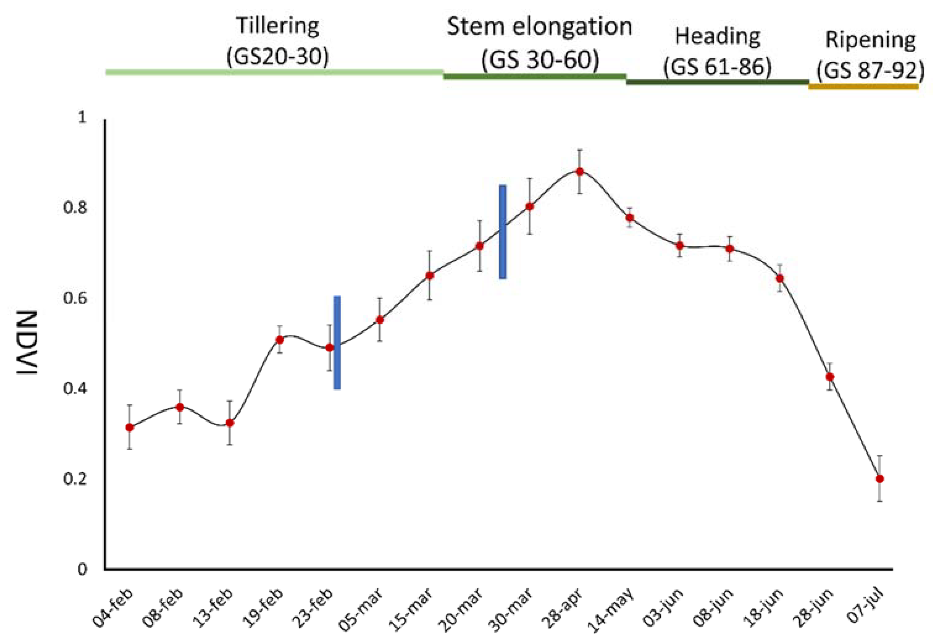
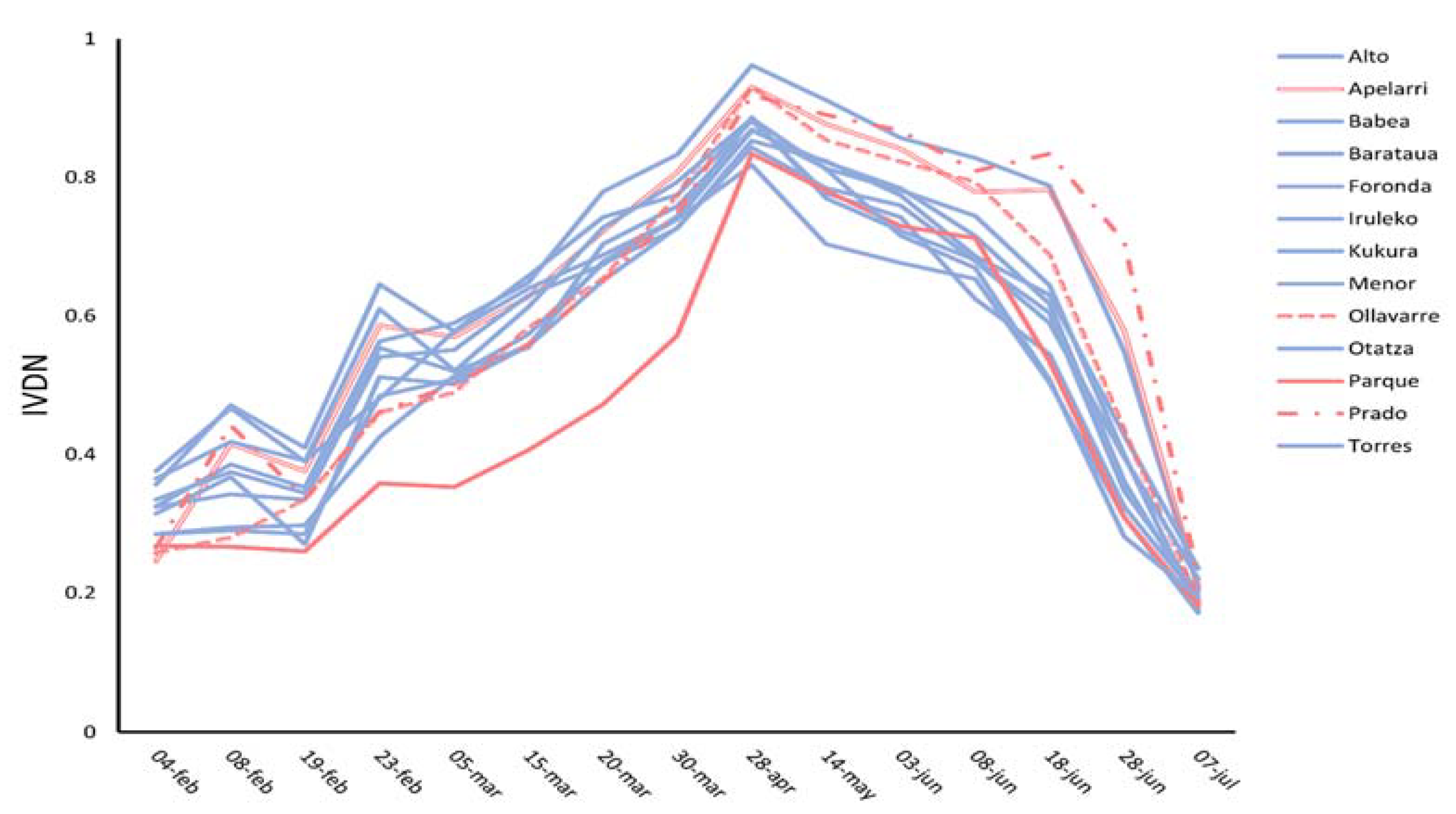
3.1. NDVI Evolution
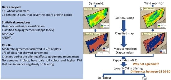
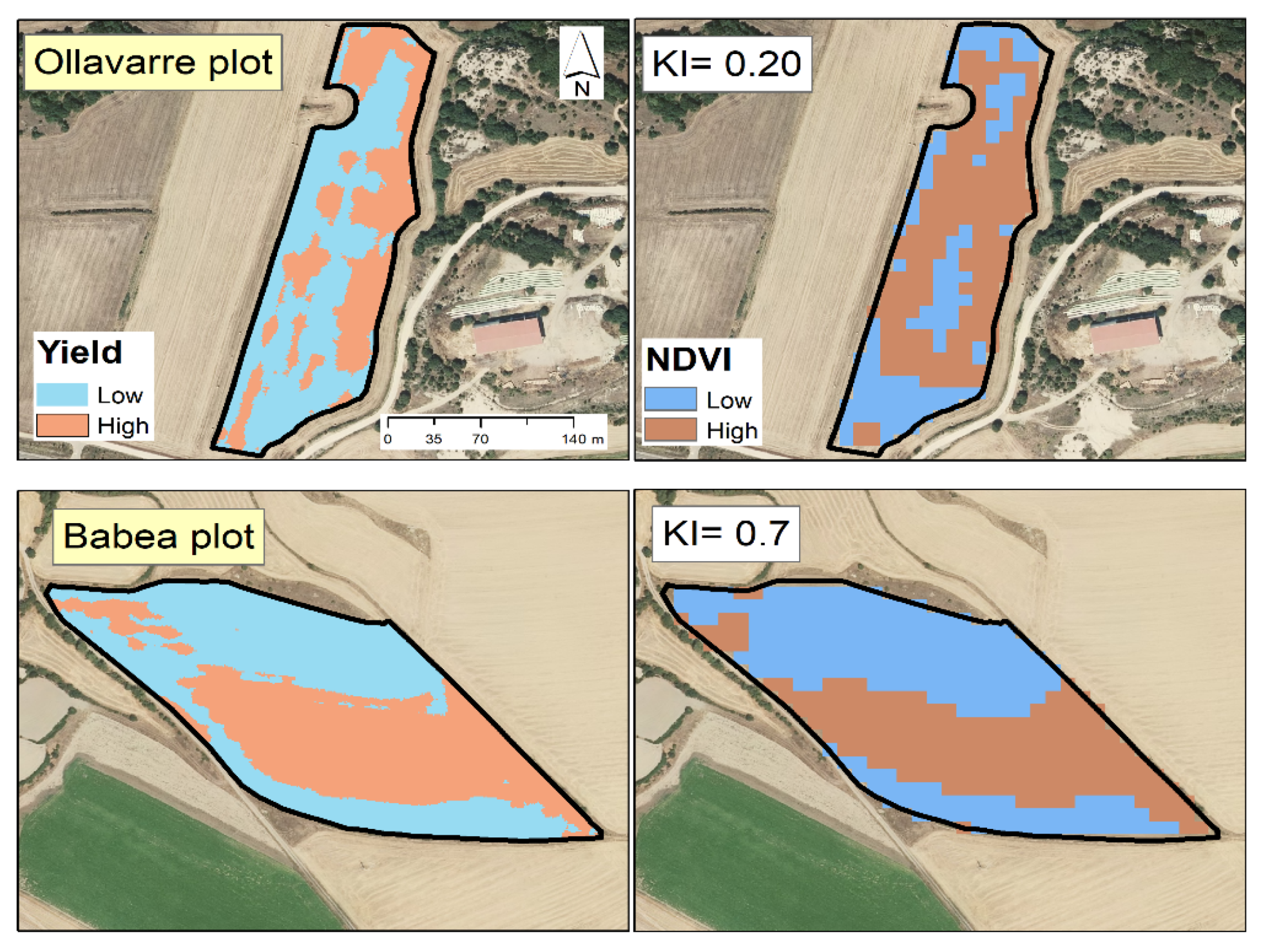
3.2. Comparison of Yield Maps and Temporal NDVI Images
3.3. Analysing the Lack of Agreement between Yield and NDVI in Some Plots
3.3.1. Multivariate Analysis of Plot Geomorphology
3.3.2. Analysis of NDVI Value using MANOVA and DDA
3.3.3. Tillering, Dissociation among Yield Map and NDVI Images
3.3.4. Why Some Plots Have a Lower NDVI during the Tillering Phase
4. Conclusions
Author Contributions
Funding
Data Availability Statement
Acknowledgments
Conflicts of Interest
References
- Zörb, C.; Ludewig, U.; Hawkesford, M.J. Perspective on wheat yield and quality with reduced nitrogen supply. Trends Plant. Sci. 2018, 23, 1029–1037. [Google Scholar] [CrossRef] [PubMed] [Green Version]
- Roy, R.N.; Finck, A.; Blair, G.J.; Tandon, H.L.S. Plant Nutrition for Food Security. A Guide for Integrated Nutrient Management. FAO Fertilizer and Plant. Nutrition Bulletin 16; Food and Agriculture Organization of the United Nations: Rome, Italy, 2006. [Google Scholar]
- Good, A.G.; Beatty, P.H. Fertilizing nature: A tragedy of excess in the commons. PLoS Biol. 2011, 9, e1001124. [Google Scholar] [CrossRef] [PubMed]
- Bruinsma, J. World Agriculture: Towards 2015/30. An. FAO Perspective 2015/30; Taylor & Francis Group: London, UK, 2000. [Google Scholar]
- Snyder, C.S.; Bruulsema, T.W.; Jensen, T.L.; Fi-en, P.E. Review of greenhouse gas emissions from crop production systems and fertilizer management effects. Agric. Ecosys. Environ. 2009, 133, 247–266. [Google Scholar] [CrossRef]
- Randall, G.; Goss, M. Nitrate Losses to Surface Water through Subsurface, Tile Drainage. In Nitrogen in the Environment: Sources, Problems, and Management; Elsevier: Amsterdam, The Netherlands, 2008. [Google Scholar]
- Khosla, R.; Fleming, K.; Delgado, J.A.; Shaver, T.M.; Westfall, D.G. Use of site-specific management zones to improve nitrogen management for precision agriculture. J. Soil Water Conserv. 2002, 57, 513–518. [Google Scholar]
- Corwin, D.L.; Lesch, S.M. Delineating site-specific management units with proximal sensors. In Geostatistical Applications for Precision Agriculture; Oliver, M.O., Ed.; Springer: New York, NY, USA, 2010; pp. 139–165. [Google Scholar]
- Schimmelpfennig, D. Farm Profits and Adoption of Precision Agriculture; Economic Research Report Number 217; U.S. Department of Agriculture, Economic Research Service: Washington, DC, USA, 2016.
- ISPA International Society of Precision Agriculture. Available online: https://www.ispag.org/about/definition (accessed on 6 February 2022).
- Van Uffelen, C.G.R.; Verhagen, J.; Bouma, J. Comparison of simulated crop yield patterns for site-specific management. Agric. Syst. 1997, 54, 207–222. [Google Scholar] [CrossRef]
- Fleming, K.L.; Westfall, D.G.; Wiens, D.W.; Brodahl, M.C. Evaluating Farmer Defined Management Zone Maps for Variable Rate Fertilizer Application. Precis. Agric. 2000, 2, 201–215. [Google Scholar] [CrossRef]
- Uribeetxebarria, U.; Daniele, E.; Escolà, A.; Arnó, J.; Martínez-Casasnovas, J.A. Spatial variability in orchards after land transformation: Consequences for precision agriculture practices. Sci. Total Environ. 2018, 635, 343–352. [Google Scholar] [CrossRef]
- Córdoba, M.A.; Bruno, C.I.; Costa, J.L.; Peralta, N.R.; Balzarini, M.G. Protocol for multivariate homogeneous zone delineation in precision agriculture. Biosyst. Eng. 2016, 143, 95–107. [Google Scholar] [CrossRef]
- Moral, F.J.; Terrón, J.M.; Silva, J.R.M.D. Delineation of management zones using mobile measurements of soil apparent electrical conductivity and multivariate geostatistical techniques. Soil Tillage Res. 2010, 106, 335–343. [Google Scholar] [CrossRef]
- Mouazen, A.M.; Kuang, B. On-line visible and near infrared spectroscopy for in-field phosphorous management. Soil Tillage Res. 2016, 155, 471–477. [Google Scholar] [CrossRef]
- Castrignanò, A.; Wong, M.T.F.; Stelluti, M.; De Benedetto, D.; Sollitto, D. Use of EMI, gamma-ray emission and GPS height as multi-sensor data for soil characterisation. Geoderma 2012, 175–176, 78–89. [Google Scholar] [CrossRef]
- Bellvert, J.; Marsal, J.; Girona, J.; Gonzalez-Dugo, V.; Fereres, E.; Ustin, S.; Zarco-Tejada, P. Airborne thermal imagery to detect the seasonal evolution of crop water status in peach, nectarine and saturn peach orchards. Remote Sens. 2016, 8, 39. [Google Scholar] [CrossRef] [Green Version]
- Sankaran, S.; Mishra, A.; Ehsani, R.; Davis, C. A review of advanced techniques for detecting plant diseases. Comput. Electron. Agric. 2010, 72, 1–13. [Google Scholar] [CrossRef]
- Maresma, Á.; Lloveras, J.; Martínez-Casasnovas, J.A. Use of Multispectral Airborne Images to Improve In-Season Nitrogen Management, Predict Grain Yield and Estimate Economic Return of Maize in Irrigated High Yielding Environments. Remote Sens. 2018, 10, 543. [Google Scholar] [CrossRef] [Green Version]
- Aranguren, M.; Castellón, A.; Aizpurua, A. Crop Sensor Based Non-destructive Estimation of Nitrogen Nutritional Status, Yield, and Grain Protein Content in Wheat. Agriculture 2020, 10, 148. [Google Scholar] [CrossRef]
- Fu, Z.; Jiang, J.; Gao, Y.; Krienke, B.; Wang, M.; Zhong, K.; Cao, Q.; Tian, Y.; Zhu, Y.; Cao, W.; et al. Wheat growth monitoring and yield estimation based on multi-rotor unmanned aerial vehicle. Remote Sens. 2020, 12, 508. [Google Scholar] [CrossRef] [Green Version]
- Gonzalez-Dugo, V.; Hernandez, P.; Solis, I.; Zarco-Tejada, P.J. Using High-Resolution Hyperspectral and Thermal Airborne Imagery to Assess Physiological Condition in the Context of Wheat Phenotyping. Remote Sens. 2015, 7, 13586–13605. [Google Scholar] [CrossRef] [Green Version]
- Skakun, S.; Vermote, E.; Franch, B.; Roger, J.C.; Kussul, N.; Ju, J.; Masek, J. Winter Wheat Yield Assessment from Landsat 8 and Sentinel-2 Data: Incorporating Surface Reflectance, Through Phenological Fitting, into Regression Yield Models. Remote Sens. 2019, 11, 1768. [Google Scholar] [CrossRef] [Green Version]
- Sishodia, R.P.; Ray, R.L.; Singh, S.K. Applications of Remote Sensing in Precision Agriculture: A Review. Remote Sens. 2020, 12, 3136. [Google Scholar] [CrossRef]
- Clevers, J.G.P.W.; Kooistra, L.; Van Den, B.; Marnix, M.M. Using Sentinel-2 Data for Retrieving LAI and Leaf and Canopy Chlorophyll Content of a Potato Crop. Remote Sens. 2017, 9, 405. [Google Scholar] [CrossRef] [Green Version]
- Mulla, D.J. Twenty-five years of remote sensing in precision agriculture: Key advances and remaining knowledge gaps. Biosyst. Eng. 2013, 114, 358–371. [Google Scholar] [CrossRef]
- Meraner, A.; Ebel, P.; Zhu, X.X.; Schmitt, M. Cloud removal in Sentinel-2 imagery using a deep residual neural network and SAR-optical data fusion. ISPRS J. Photogramm. 2020, 166, 333–346. [Google Scholar] [CrossRef] [PubMed]
- Huang, X.; Liu, J.; Zhu, W.; Atzberger, C.; Liu, Q. The Optimal Threshold and Vegetation Index Time Series for Retrieving Crop Phenology Based on a Modified Dynamic Threshold Method. Remote Sens. 2019, 11, 2725. [Google Scholar] [CrossRef] [Green Version]
- Potgieter, A.B.; Apan, A.; Dunn, P.; Hammer, G. Estimating crop area using seasonal time series of enhanced vegetation index from MODIS satellite imagery. Aust. J. Agric. Res. 2007, 58, 316–325. [Google Scholar] [CrossRef] [Green Version]
- Magney, T.S.; Eitel, J.U.H.; Huggins, D.R.; Vierling, L.A. Proximal NDVI derived phenology improves in-season predictions of wheat quantity and quality. Agric. For. Meteorol. 2016, 217, 46–60. [Google Scholar] [CrossRef]
- Rouse, J.W., Jr.; Haas, R.H.; Deering, D.W.; Schell, J.A.; Harlan, J.C. Monitoring the Vernal Advancement and Retrogradation (GreenWave Effect) of Natural Vegetation; NASA/GSFC Type III Final Report; NASA/GSFC: Greenbelt, MD, USA, 1974; p. 371.
- Vallentin, C.; Harfenmeister, K.; Itzerott, S.; Kleinschmit, B.; Conrad, C.; Spengler, D. Suitability of satellite remote sensing data for yield estimation in northeast Germany. Precis. Agric. 2022, 23, 52–82. [Google Scholar] [CrossRef]
- Index Database. Available online: https://www.indexdatabase.de/db/is.php?sensor_id=96 (accessed on 16 June 2021).
- Baret, F.; Guyot, G. Potentials and Limits of Vegetation LAI and APAR Assessment. Remote Sens. Environ. 1991, 35, 161–173. [Google Scholar] [CrossRef]
- Bhandari, M.; Baker, S.; Rudd, J.C.; Ibrahim, A.M.H.; Chang, A.; Xue, Q.; Jung, J.; Landivar, J.; Auvermann, B. Assessing the Effect of Drought on Winter Wheat Growth Using Unmanned Aerial System (UAS)-Based Phenotyping. Remote Sens. 2021, 13, 1144. [Google Scholar] [CrossRef]
- David, J.B. Wheat phenomics in the field by RapidScan: NDVI vs. NDRE. Isr. J. Plant Sci. 2017, 64, 41–54. [Google Scholar]
- Rasmussen, J.; Azim, S.; Boldsen, S.K.; Nitschke, T.; Jensen, S.M.; Nielsen, J.; Christensen, S. The challenge of reproducing remote sensing data from satellites and unmanned aerial vehicles (UAVs) in the context of management zones and precision agriculture. Precis. Agric. 2021, 22, 834–851. [Google Scholar] [CrossRef]
- Panek, E.; Gozdowski, D.; Stępień, M.; Samborski, S.; Ruciński, D.; Buszke, B. Within-Field Relationships between Satellite-Derived Vegetation Indices, Grain Yield and Spike Number of Winter Wheat and Triticale. Agronomy 2020, 10, 1842. [Google Scholar] [CrossRef]
- Aranguren, M.; Castellón, A.; Aizpurua, A. Crop Sensor-Based In-Season Nitrogen Management of Wheat with Manure Application. Remote Sens. 2019, 11, 1094. [Google Scholar] [CrossRef] [Green Version]
- Ravier, C.; Jeuffroy, M.-H.; Meynard, J.-M. Mismatch between a science-based decision tool and its use: The case of the balance-sheet method for nitrogen fertilization in France. NJAS-Wagening. J. Life Sci. 2016, 79, 31–40. [Google Scholar] [CrossRef]
- Ilsemann, J.; Goeb, S.; Bachmann, J. How many soil samples are necessary to obtain a reliable estimate of mean nitrate concentrations in an agricultural field? J. Plant Nutr. Soil Sci. 2001, 164, 585–590. [Google Scholar] [CrossRef]
- Ortuzar-Iragorri, M.A.; Aizpurua, A.; Castellón, A.; Alonso, A.; Estavillo, J.M.; Besga, G. Use of an N-tester chlorophyll meter to tune a late third nitrogen application to wheat under humid Mediterranean conditions. J. Plant Nutr. 2018, 41, 627–635. [Google Scholar] [CrossRef]
- Unamunzaga, O.; Aizpurua, A.; Artetxe, A.; Besga, G.; Castroviejo, L.; Blanco, F.; de la Llera, I.; Ramos, L.; Astola, G. Asis-tencia Técnica Para la Caracterización Agrológica del Suelo Rústico del Municipio de Vitoria-Gasteiz. Available online: https://docplayer.es/amp/152712108-Asistencia-tecnica-para-la-caracterizacion-agrologica-del-suelo-rustico-del-municipio-de-vitoria-gasteiz.html (accessed on 21 March 2021). (In Spanish).
- Beck, H.E.; Zimmermann, N.E.; McVicar, T.R.; Vergopolan, N.; Berg, A.; Wood, E.F. Data descriptor: Present and future Köppen–Geiger climate classification maps at 1-km resolution. Sci. Data 2018, 5, 180–214. [Google Scholar] [CrossRef] [Green Version]
- Taylor, J.; McBratney, A.; Whelan, B. Establishing management classes for broadacre agricultural production. Agron. J. 2007, 99, 1366–1376. [Google Scholar] [CrossRef]
- Zhang, C.; Luo, L.; Xu, W.; Ledwith, V. Use of local Moran’s I and GIS to identify pollution hotspots of Pb in urban soils of Galway, Ireland. Sci. Total Environ. 2008, 398, 212–221. [Google Scholar] [CrossRef]
- Drusch, M.; Del Bello, U.; Carlier, S.; Colin, O.; Fernandez, V.; Gascon, F.; Hoersch, B.; Isola, C.; Laberinti, P.; Martimort, P.; et al. Sentinel-2: ESA’s optical high-resolution mission for GMES operational services. Remote Sens. Environ. 2012, 120, 25–36. [Google Scholar] [CrossRef]
- Zadoks, J.C.; Chang, T.T.; Zonzak, C.F. A decimal code for the growth stages of cereals. Weed Res. 1974, 14, 415–421. [Google Scholar] [CrossRef]
- Brisson, N.; Launay, M.; Mary, B.; Beaudoin, N. Conceptual Basis, Formalisations and Parameterization of the Stics Crop Model; Quae: Paris, France, 2009; p. 304. [Google Scholar]
- Official Basque Government Spatial Data Page. Available online: www.geoeuskadi.com (accessed on 8 June 2021).
- Grabs, T.; Seibert, J.; Bishop, K.; Laudon, H. Modelling spatial patterns of saturated areas: A comparison of the topographic wetness index and a dynamic distributed model. J. Hydrol. 2009, 373, 15–23. [Google Scholar] [CrossRef] [Green Version]
- Sørensen, R.; Zinko, U.; Seibert, J. On the calculation of the topographic wetness index: Evaluation of different methods based on field observations. Hydrol. Earth Syst. Sci. Discuss. 2006, 10, 101–112. [Google Scholar] [CrossRef] [Green Version]
- Guastaferro, F.; Castrignanò, A.; De Benedetto, D.; Sollitto, D.; Troccoli, A.; Cafarelli, B.A. Comparison of different algorithms for the delineation of management zones. Precis. Agric. 2010, 11, 600–620. [Google Scholar] [CrossRef]
- Cohen, J. A coefficient of agreement for nominal scales. Educ. Psychol. Meas. 1960, 20, 37–46. [Google Scholar] [CrossRef]
- Landis, J.R.; Koch, G.G. The measurement of observer agreement for categorical data. Biometrics 1977, 33, 159–174. [Google Scholar] [CrossRef] [Green Version]
- Stemler, S.E.A. Comparison of Consensus, Consistency, and Measurement Approaches to Estimating Interrater Reliability. Pract. Assess. Res. Eval. 2004, 9, 1–12. [Google Scholar] [CrossRef]
- McHugh, M.L. Interrater reliability: The kappa statistic. Biochem. Med. 2012, 22, 276–282. [Google Scholar] [CrossRef]
- Ping, J.L.; Green, C.J.; Bronson, K.F.; Zartman, R.E.; Dobermann, A. Delineating potential management zones for cotton based on yields and soil properties. Soil Sci. 2005, 170, 371–385. [Google Scholar] [CrossRef]
- Huberty, C.J.; Olejnik, S. Applied MANOVA and Discriminant Analysis; John Wiley & Sons: Hoboken, NJ, USA, 2006. [Google Scholar]
- Thomas, D.R. Interpreting discriminant functions. A data analytic approach. Multivar. Behav. Res. 1992, 27, 335–362. [Google Scholar] [CrossRef]
- Uribeetxebarria, A.; Arnó, J.; Escolà, A.; Martínez-Casasnovas, J.A. Apparent electrical conductivity and multivariate analysis of soil properties to assess soil constraints in orchards affected by previous parcelling. Geoderma 2018, 319, 185–193. [Google Scholar] [CrossRef] [Green Version]
- Eitel, J.U.H.; Long, D.S.; Gessler, P.E.; Smith, A.M.S. Using in-situ measurements to evaluate the new RapidEyeTM satellite series for prediction of wheat nitrogen status. Int. J. Remote Sens. 2007, 28, 4183–4190. [Google Scholar] [CrossRef]
- Anderegg, J.; Yu, K.; Aasen, H.; Walter, A.; Liebisch, F.; Hund, A. Spectral Vegetation Indices to Track Senescence Dynamics in Diverse Wheat Germplasm. Front. Plant Sci. 2020, 10, 1749. [Google Scholar] [CrossRef] [PubMed] [Green Version]
- Labus, M.P.; Nielsen, G.A.; Lawrence, R.L.; Engel, R. Wheat yield estimates using multi-temporal NDVI satellite imagery. Int. J. Remote Sens. 2002, 23, 4169–4180. [Google Scholar] [CrossRef]
- Hunt, M.L.; Blackburn, G.A.; Carrasco, L.; Redhead, J.W.; Rowland, C.S. High resolution wheat yield mapping using Sentinel-2. Remote Sens. Environ. 2019, 233, 111410. [Google Scholar] [CrossRef]
- Martí, J.; Bort, J.; Slafer, G.; Araus, J. Can wheat yield be assessed by early measurements of normalized difference vegetation index? Ann. Appl. Biol. 2007, 150, 253–257. [Google Scholar] [CrossRef]
- Royo, C.; Aparicio, N.; Villegas, D.; Casadesus, J.; Araus, J.L.; Aparicio, N.; Villegas, D.; Casadesus, J. Usefulness of Spectral Reflectance Indices as Durum Wheat Yield Predictors under Contrasting Mediterranean Conditions. Int. J. Remote Sens. 2003, 24, 4403–4419. [Google Scholar] [CrossRef]
- Babar, M.A.; Reynolds, M.P.; van Ginkel, M.; Klatt, A.R.; Raun, W.R.; Stone, M.L. Spectral reflectance indices as a potential indirect selection criteria for wheat yield under irrigation. Crop Sci. 2006, 46, 578–588. [Google Scholar] [CrossRef]
- Naser, M.A.; Khosla, R.; Longchamps, L.; Dahal, S. Using NDVI to Differentiate Wheat Genotypes Productivity under Dryland and Irrigated Conditions. Remote Sens. 2020, 12, 824. [Google Scholar] [CrossRef] [Green Version]
- De Benedetto, D.; Castrignanò, A.; Rinaldi, M.; Ruggieri, S.; Santoro, F.; Figorito, B.; Gualano, S.; Diacono, M.; Tamborrino, R. An approach for delineating homogeneous zones by using multi-sensor data. Geoderma 2013, 199, 117–127. [Google Scholar] [CrossRef]
- Stadler, A.; Rudolph, S.; Kupisch, M.; Langensiepen, M.; van der Kruk, J.; Ewert, F. Quantifying the effects of soil variability on crop growth using apparent soil electrical conductivity measurements. Eur. J. Agron. 2015, 64, 8–20. [Google Scholar] [CrossRef]
- Satorre, E.H.; Slafer, G.A. Wheat. Ecology and Physiology of Yield Determination; CRC Press: New York, NY, USA, 1999. [Google Scholar]
- Serrano, L.; Filella, I.; Pen, J. Remote Sensing of Biomass and Yield of Winter Wheat under Diferent Nitrogen Supplies. Crop Sci. 2000, 40, 723–731. [Google Scholar] [CrossRef] [Green Version]
- Slafer, G.A.; Buck, H.T. Physiological Determination of Major Wheat Yield Components in Wheat Production in Stressed Environments; Buck, H.T., Nisi, J.E., Salomón, N., Eds.; Springer: Dordrecht, The Netherlands, 2007; pp. 557–565. [Google Scholar]
- Klepper, B.; Rickman, R.W.; Peterson, C.M. Quantitative characterization of vegetative development in small cereal grains. Agron. J. 1982, 74, 789–792. [Google Scholar] [CrossRef]
- AHDB Cereales & Oleaginosas. Wheat Growth Guide; AHDB Cereales & Oleaginosas: Warwickshire, UK, 2018. [Google Scholar]
- Kirby, E.J.M. Development of the Cereal Plant. In The Yield of 617 the Cereals; Wright, D.W., Ed.; Royal Agricultural Society of England: London, UK, 1983; pp. 1–3. [Google Scholar]
- Tilley, M.S.; Heiniger, R.W.; Crozier, C.R. Improving Winter Wheat Yield in the Southeast by Examining the Development and Mortality of Fall, Winter, and Spring Tillers Using Different Seed Populations and Nitrogen Management Strategies. Master’s Thesis, North Carolina State University, Raleigh, NC, USA, 2015. [Google Scholar]
- Gallanger, J.N.; Biscoe, P.V. Radiation absorption, growth, and yield of cereals. J. Agric. Sci. 1978, 91, 47–60. [Google Scholar] [CrossRef]
- Shen, Y.; Guo, S. Effects of photoperiod on wheat growth, development and yield in CELSS. Acta Astronaut. 2014, 105, 24–29. [Google Scholar] [CrossRef]
- Lindstrom, M.J.; Papendick, R.I.; Koehler, F.E. A model to predict winter wheat emergence as affected by soil temperature, water potential and depth of planting. Agron. J. 1976, 68, 137–141. [Google Scholar] [CrossRef]
- Colmer, T.D.; Voesenek, L.A.C.J. Flooding tolerance: Suites of plant traits invariable environments. Funct. Plant Biol. 2009, 36, 665–681. [Google Scholar] [CrossRef]
- Dickin, E.; Wright, D. The effects of winter waterlogging and summer drought on the growth and yield of winter wheat (Triticum aestivum L.). Eur. J. Agron. 2008, 28, 234–244. [Google Scholar] [CrossRef]
- Cerro, I.; Antigüedad, I.; Srinavasan, R.; Sauvage, S.; Volk, M.; Sanchez-Perez, J.M. Simulating land management options to reduce nitrate pollution in an agricultural watershed dominated by an alluvial aquifer. J. Environ Qual. 2014, 43, 67–74. [Google Scholar] [CrossRef] [PubMed] [Green Version]
- Martinez, M.; García, M.C.; Antigüedad, I.; Sánchez-Perez, J.M.; Aizpurua, A. Funcionalidad de las zonas húmedas del cinturón periurbano de Vitoria-Gasteiz: Consecuencias sobre la desnitrificación de las aguas subterráneas. Temas Investig. Ne Zona No Satura. 2001, 26, 147–156. [Google Scholar]
- Nwankwo, C.; Ogugurue, D. An investigation of temperature variation at soil depths in parts of Southern Nigeria. Am. J. Environ. Sci. 2012, 2, 142–147. [Google Scholar] [CrossRef] [Green Version]
- Onwuka, B.; Mang, M. Effects of soil temperature on some soil properties and plant growth. Adv. Plants Agric Res. 2018, 8, 34–37. [Google Scholar] [CrossRef]
- Arguello, M.N.; Mason, R.E.; Roberts, T.L.; Subramanian, N.; Acuña, A.; Addison, C.K.; Lozada, D.N.; Miller, R.G.; Gbur, E. Performance of soft red winter wheat subjected to field soil waterlogging: Grain yield and yield components. Field Crops Res. 2016, 194, 57–64. [Google Scholar] [CrossRef] [Green Version]
- Moragues, M.; García del Moral, L.F.; Moralejo, M.; Royo, C. Yield formation strategies of durum wheat landraces with distinct pattern of dispersal within the Mediterranean basin: II. Biomass production and allocation. Field Crop Res. 2006, 95, 182–193. [Google Scholar] [CrossRef]


| Labor | Date | Variety/Product | Dose (kg ha−1) |
|---|---|---|---|
| Sowing | 24 November 2018 | Filon | 230 |
| Fertilization | 30 December 2018 | Blending (13, 20, 30) | 410 |
| Fertilization | 26 February 2019 | ANC | 220 |
| Fertilization | 25 March 2019 | ANC | 210 |
| Plot | Yield (t ha−1) | Area (ha) | No. Sample Points | Soil Type | Elevation (m) | Slope (%) | CV (%) of Slope |
|---|---|---|---|---|---|---|---|
| Alto | 8.6 | 5.1 | 426 | Quaternary | 502 | 1.03 | 1.3 |
| Apelarri | 7.8 | 2.6 | 207 | Quaternary | 508 | 1.09 | 0.6 |
| Babea | 6.7 | 3.8 | 323 | Quaternary | 521 | 6.44 | 2.94 |
| Baratua | 5.6 | 2.7 | 217 | Quaternary | 511 | 1.24 | 0.87 |
| Foronda | 6.4 | 3.2 | 254 | Quaternary | 513 | 0.95 | 0.52 |
| Iruleku | 7.4 | 4.1 | 346 | Cretaceous | 534 | 2.45 | 2.39 |
| Kukura | 6.3 | 5.0 | 417 | Quaternary | 508 | 1.53 | 0.82 |
| Menor | 5.2 | 4.6 | 358 | Cretaceous | 538 | 4.12 | 1.43 |
| Ollavarre | 4.6 | 4.3 | 353 | Cretaceous | 554 | 6.12 | 2.67 |
| Otatza | 6.3 | 3.0 | 246 | Cretaceous | 541 | 4.46 | 1.66 |
| Parque | 4.7 | 5.2 | 246 | Cretaceous | 531 | 5.83 | 2.67 |
| Prado | 7.1 | 2.5 | 208 | Quaternary | 501 | 0.91 | 0.56 |
| Torres | 7.1 | 12.2 | 916 | Cretaceous | 511 | 9.53 | 6.83 |
| Data | Sentinel-2 Tile |
|---|---|
| 4 February | S2B_MSIL2A_20190204T110439_N0211_R094_T30TWN |
| 8 February | S2A_MSIL2A_20190208T110221_N0211_R094_T30TWN |
| 13 February | S2A_MSIL2A_20190213T110149_N0211_R094_T30TWN |
| 19 February | S2A_MSIL2A_20190218T110111_N0211_R094_T30TWN |
| 23 February | S2B_MSIL2A_20190223T110039_N0211_R094_T30TWN |
| 5 March | S2A_MSIL2A_20190228T110001_N0211_R094_T30TWN |
| 15 March | S2B_MSIL2A_20190315T105819_N0211_R094_T30TWN |
| 20 March | S2A_MSIL2A_20190320T105741_N0211_R094_T30TWN |
| 30 March | S2A_MSIL2A_20190330T105631_N0211_R094_T30TWN |
| 29 April | S2A_MSIL2A_20190429T105621_N0211_R094_T30TWN |
| 14 May | S2B_MSIL2A_20190514T105629_N0212_R094_T30TWN |
| 3 June | S2B_MSIL2A_20190603T105629_N0212_R094_T30TWN |
| 8 June | S2A_MSIL2A_20190608T105621_N0212_R094_T30TWN |
| 18 June | S2A_MSIL2A_20190618T105621_N0212_R094_T30TWN |
| 28 June | S2A_MSIL2A_20190628T105621_N0212_R094_T30TWN |
| 18 July | S2A_MSIL2A_20190718T105621_N0213_R094_T30TWN |
| Data | Alto | Apelarri | Babea | Baratua | Iruleku | Kukura | Menor | Ollavarre | Otatza | Parque | Prado | Torres | Foronda |
|---|---|---|---|---|---|---|---|---|---|---|---|---|---|
| 4 February | - | - | - | 0.26 | 0.32 | - | −0.1 | 0 | 0 | 0 | −0.16 | −0.04 | −0.26 |
| 8 February | −0.24 | - | 0.2 | 0.17 | - | 0.32 | - | −0.27 | 0.16 | 0.18 | −0.13 | −0.09 | 0.19 |
| 19 February | −0.31 | −0.23 | 0.39 | 0.29 | - | - | - | −0.27 | 0 | 0.19 | −0.17 | −0.01 | - |
| 23 February | −0.26 | - | 0.3 | 0.29 | 0.24 | 0.27 | - | −0.29 | 0.14 | - | −0.26 | −0.06 | - |
| 5 March | −0.19 | −0.12 | 0.55 | 0.4 | 0.62 | 0.46 | - | −0.25 | - | - | −0.16 | 0.07 | - |
| 15 March | - | - | 0.55 | 0.44 | - | 0.52 | - | −0.22 | - | - | −0.12 | 0.07 | 0.28 |
| 20 March | - | −0.12 | - | - | - | - | - | - | - | - | - | - | - |
| 30 March | 0.15 | - | 0.41 | 0.56 | - | 0.45 | - | - | 0.35 | 0.3 | −0.11 | 0.15 | - |
| 28 April | 0.21 | - | 0.66 | 0.52 | 0.17 | 0.44 | 0.6 | 0.17 | 0.42 | 0.21 | 0.08 | 0.12 | - |
| 14 May | 0.27 | - | 0.55 | 0.51 | - | 0.44 | 0.55 | 0.2 | - | 0.13 | 0.17 | 0.16 | 0.35 |
| 3 June | 0.35 | 0.34 | 0.54 | 0.48 | 0.24 | 0.55 | 0.55 | 0.16 | 0.52 | 0.21 | 015 | 0.32 | 0.55 |
| 8 June | 0.33 | 0.32 | 0.7 | 0.45 | 0.25 | 0.5 | 0.63 | 0.16 | 0.5 | 0.31 | 0.10 | 0.39 | 0.61 |
| 18 June | 0.39 | 0.31 | 0.7 | 0.5 | 0.25 | 0.58 | 0.7 | 0.19 | 0.49 | 0.32 | 0.11 | 0.56 | 0.62 |
| 28 June | 0.33 | 0.32 | 0.65 | 0.43 | - | 0.63 | - | 0.15 | 0.45 | 0.26 | 0.05 | 0.34 | 0.62 |
| Properties | Unrelated Group | Related Group |
|---|---|---|
| Plot number (n) | 4 | 9 |
| Elevation (m) | 519.88 ± 14.3 | 523.50 ± 24.3 |
| Slope (%) | 3.55 ± 3.0 | 3.48 ± 2.8 |
| Slope CV (%) | 2.08 ± 1.9 | 1.62 ± 1.2 |
| Phenological Stages | Vegetation Index | Date | Discriminant Analysis (DDA) | ||
|---|---|---|---|---|---|
| SDFC | SC | Parallel DRC | |||
| Tillering (GS 20–G S30) | NDVI | 4 February | 0.32 | 0.16 | 0.05 |
| NDVI | 8 February | −1.61 | 0.08 | −0.13 * | |
| NDVI | 19 February | 2.92 | 0.34 | 1.01 * | |
| NDVI | 23 February | −0.60 | 0.23 | −0.14 * | |
| NDVI | 5 March | −0.65 | 0.24 | −0.15 * | |
| NDVI | 15 March | 1.58 | 0.20 | 0.32 * | |
| NDVI | 20 March | 0.09 | 0.17 | 0.02 | |
| Stem Elongation (GS 31–GS 60) | NDVI | 30 March | −0.68 | −0.07 | 0.05 |
| NDVI | 28 April | 0.05 | 0.10 | 0.01 | |
| NDVI | 14 May | −1.81 | −0.01 | 0.01 | |
| Heading (GS 61–GS 86) | NDVI | 3 June | 1.06 | −0.02 | −0.02 |
| NDVI | 8 June | −1.11 | −0.03 | 0.04 | |
| NDVI | 18 June | 0.71 | −0.03 | −0.02 | |
| Ripening (GS 87–GS 92) | NDVI | 28 June | −0.15 | −0.11 | 0.02 |
Publisher’s Note: MDPI stays neutral with regard to jurisdictional claims in published maps and institutional affiliations. |
© 2022 by the authors. Licensee MDPI, Basel, Switzerland. This article is an open access article distributed under the terms and conditions of the Creative Commons Attribution (CC BY) license (https://creativecommons.org/licenses/by/4.0/).
Share and Cite
Uribeetxebarria, A.; Castellón, A.; Aizpurua, A. A First Approach to Determine If It Is Possible to Delineate In-Season N Fertilization Maps for Wheat Using NDVI Derived from Sentinel-2. Remote Sens. 2022, 14, 2872. https://doi.org/10.3390/rs14122872
Uribeetxebarria A, Castellón A, Aizpurua A. A First Approach to Determine If It Is Possible to Delineate In-Season N Fertilization Maps for Wheat Using NDVI Derived from Sentinel-2. Remote Sensing. 2022; 14(12):2872. https://doi.org/10.3390/rs14122872
Chicago/Turabian StyleUribeetxebarria, Asier, Ander Castellón, and Ana Aizpurua. 2022. "A First Approach to Determine If It Is Possible to Delineate In-Season N Fertilization Maps for Wheat Using NDVI Derived from Sentinel-2" Remote Sensing 14, no. 12: 2872. https://doi.org/10.3390/rs14122872