Application and Comparison of the MODIS-Derived Enhanced Vegetation Index to VIIRS, Landsat 5 TM and Landsat 8 OLI Platforms: A Case Study in the Arid Colorado River Delta, Mexico

 , and
, and
Abstract
:1. Introduction
2. Materials and Methods
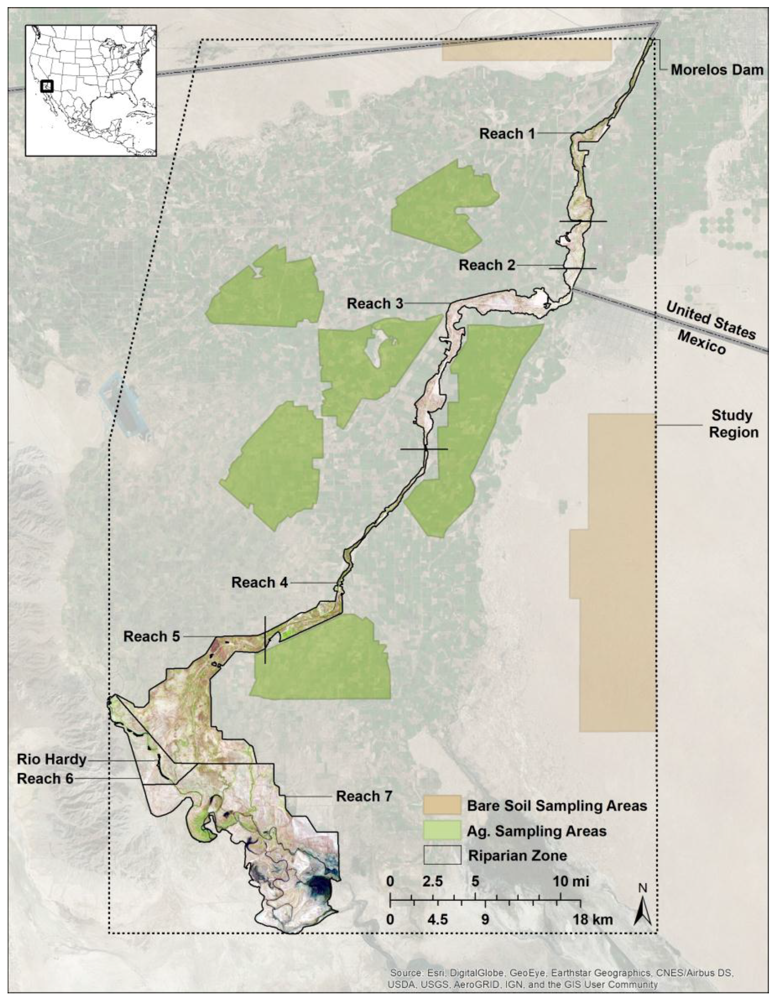
2.1. Study Region
2.2. Mask Development and Data Acquisition
2.3. Data Pre-Processing
2.3.1. MODIS and VIIRS EVI
2.3.2. Landsat EVI
2.4. Data Processing and Analysis
3. Results
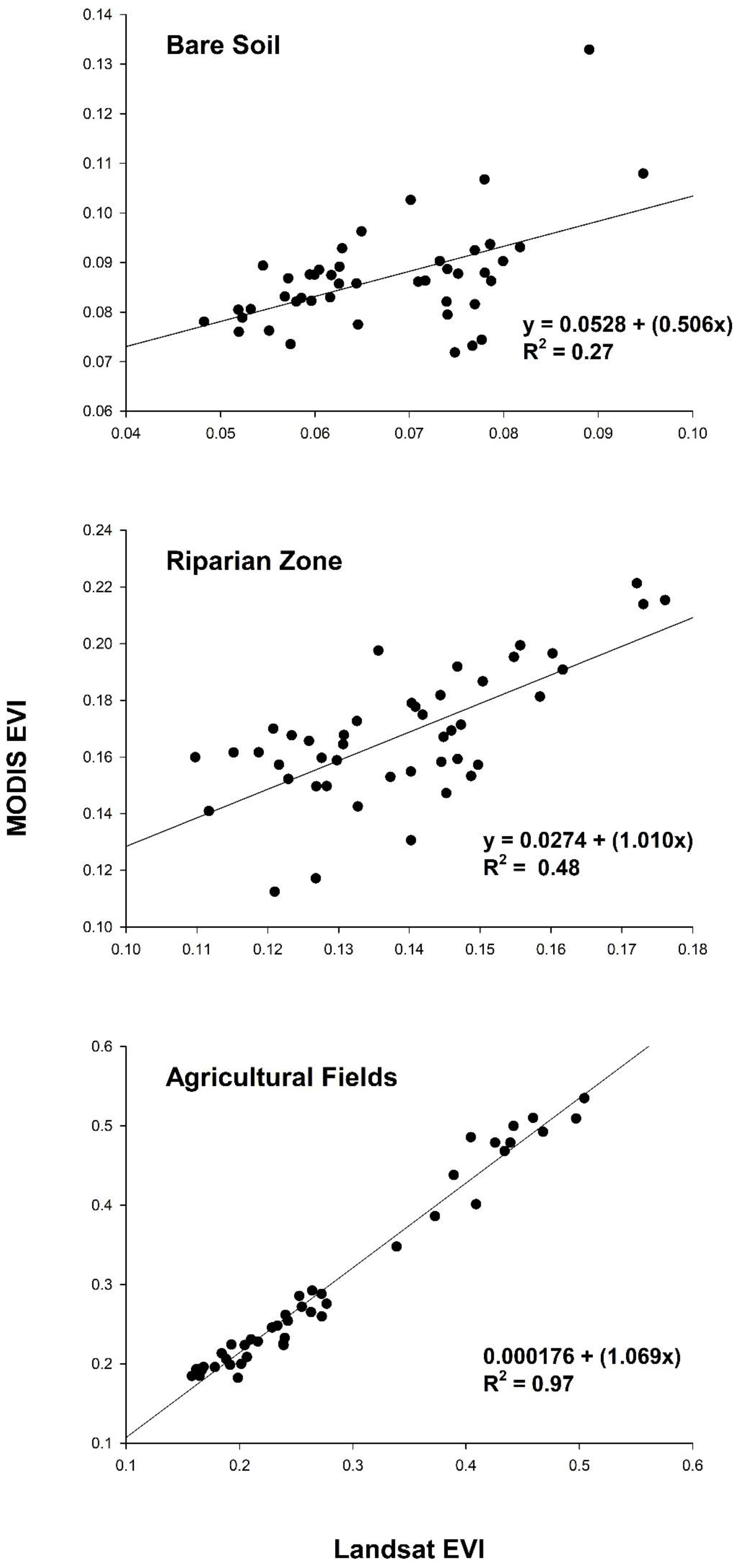
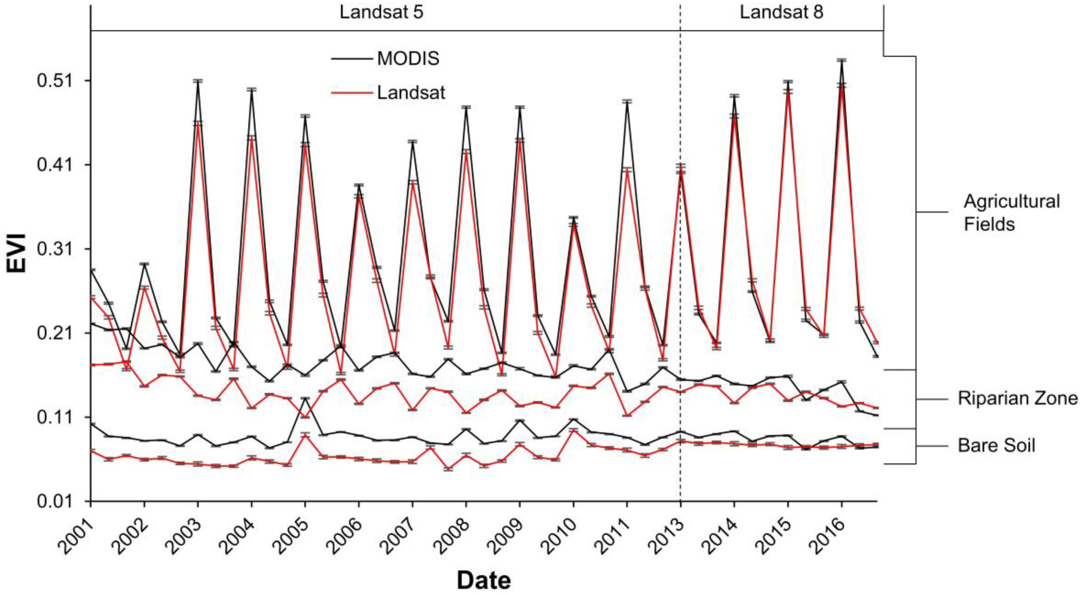
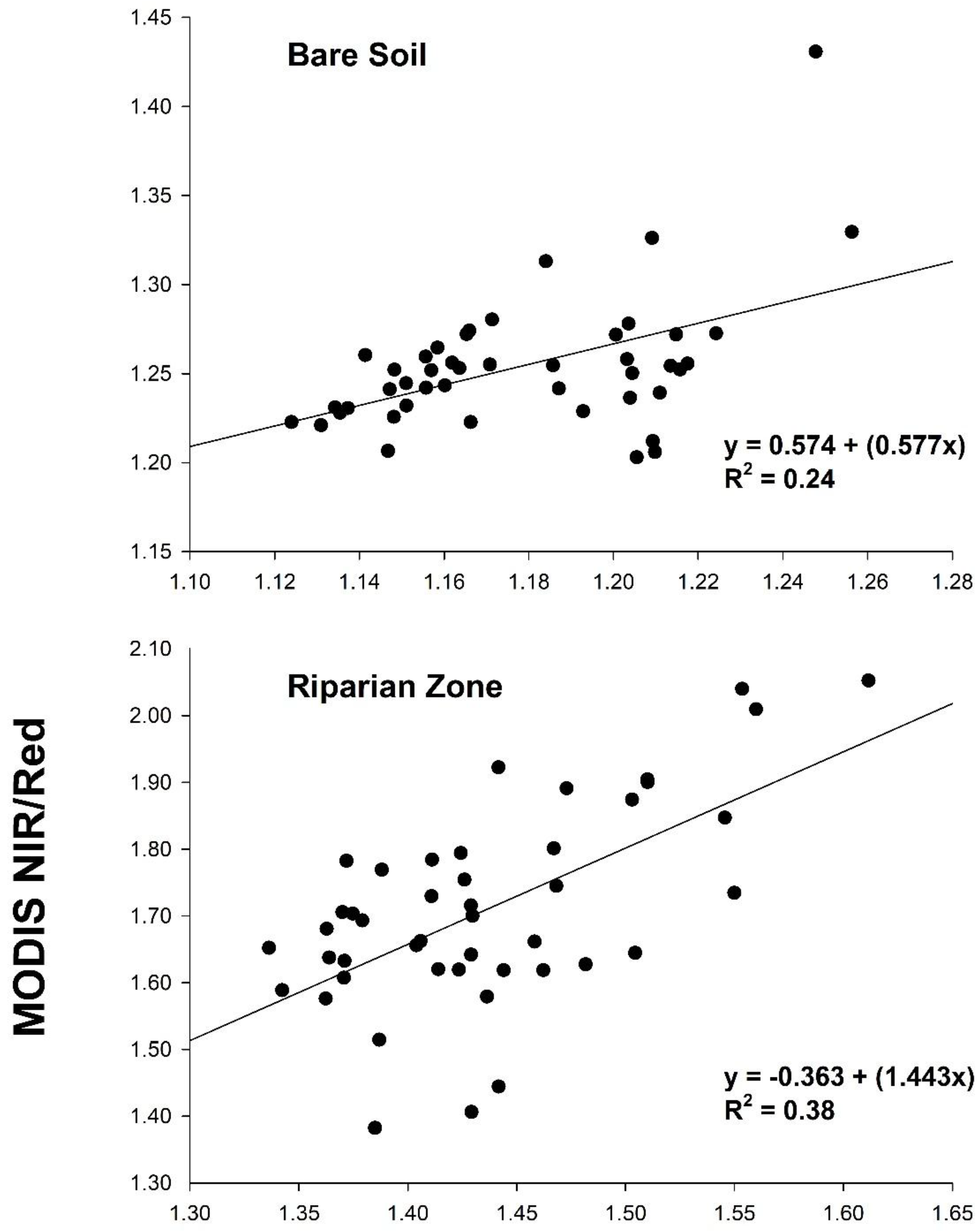
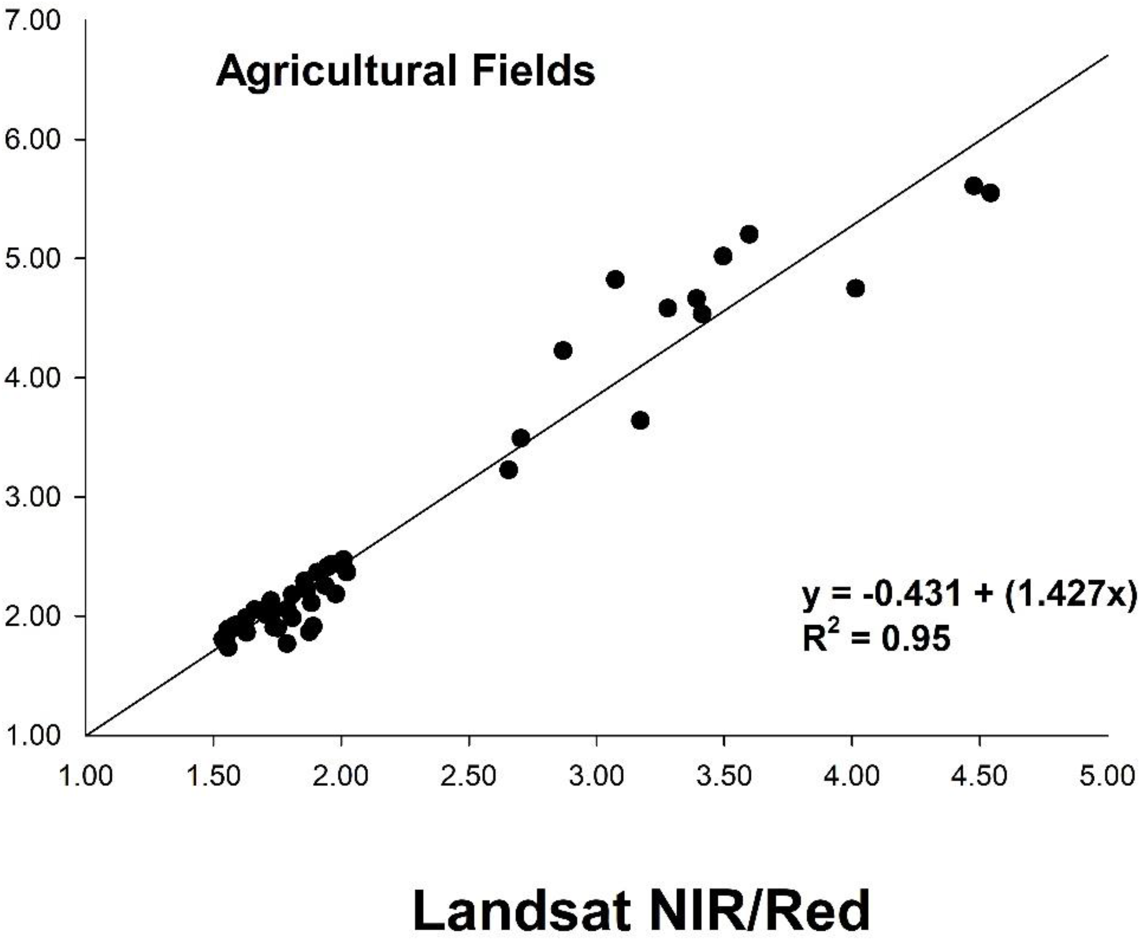
3.1. Comparison by Study Region
3.2. Comparisons by River Reach
4. Discussion
4.1. Comparison by Study Region
4.2. Comparisons by River Reach
5. Conclusions
Author Contributions
Funding
Acknowledgments
Conflicts of Interest
References
- Burgan, R.E.; Hartford, R.A. Monitoring Vegetation Greenness with Satellite Data; US Department of Agriculture, Forest Service, Intermountain Research Station: Ogden, UT, USA, 1993.
- Tucker, C.J. Red and photographic infrared linear combinations for monitoring vegetation. Remote Sens. Environ. 1979, 8, 127–150. [Google Scholar] [CrossRef]
- Fensholt, R.; Langanke, T.; Rasmussen, K.; Reenberg, A.; Prince, S.D.; Tucker, C.; Scholes, R.J.; Le, Q.B.; Bondeau, A.; Eastman, R.; et al. Greenness in semi-arid areas across the globe 1981–2007—An earth observing satellite based analysis of trends and drivers. Remote Sens. Environ. 2012, 121, 144–158. [Google Scholar] [CrossRef]
- Huete, A.; Didan, K.; Miura, T.; Rodriguez, E.P.; Gao, X.; Ferreira, L.G. Overview of the radiometric and biophysical performance of the MODIS vegetation indices. Remote Sens. Environ. 2002, 83, 195–213. [Google Scholar] [CrossRef]
- Myneni, R.B.; Ramakrishna, R.; Nemani, R.; Running, S.W. Estimation of global leaf area index and absorbed par using radiative transfer models. IEEE Trans. Geosci. Remote Sens. 1997, 35, 1380–1393. [Google Scholar] [CrossRef]
- Stow, D.; Petersen, A.; Hope, A.; Engstrom, R.; Coulter, L. Greenness trends of arctic tundra vegetation in the 1990s: Comparison of two NDVI data sets from NOAA AVHRR systems. Int. J. Remote Sens. 2007, 28, 4807–4822. [Google Scholar] [CrossRef]
- Todd, S.W.; Hoffer, R.M.; Milchunas, D.G. Biomass estimation on grazed and ungrazed rangelands using spectral indices. Int. J. Remote Sens. 1998, 19, 427–438. [Google Scholar] [CrossRef]
- Xiao, J.; Moody, A. A comparison of methods for estimating fractional green vegetation cover within a desert-to-upland transition zone in central New Mexico, USA. Remote Sens. Environ. 2005, 98, 237–250. [Google Scholar] [CrossRef]
- Huete, A.R. A soil-adjusted vegetation index (savi). Remote Sens. Environ. 1988, 25, 295–309. [Google Scholar] [CrossRef]
- Qi, J.; Chehbouni, A.; Huete, A.R.; Kerr, Y.H.; Sorooshian, S. A modified soil adjusted vegetation index. Remote Sens. Environ. 1994, 48, 119–126. [Google Scholar] [CrossRef]
- Huete, A.R.; Liu, H.Q.; Batchily, K.; Van Leeuwen, W.J. A comparison of vegetation indices over a global set of TM images for EOS-MODIS. Remote Sens. Environ. 1997, 59, 440–451. [Google Scholar] [CrossRef]
- Huete, A.; Didan, K.; van Leeuwen, W.; Miura, T.; Glenn, E. Modis vegetation indices. In Land Remote Sensing and Global Environmental Change; Springer: New York, NY, USA, 2011; Volume 11, pp. 579–602. [Google Scholar]
- Miura, T.; Huete, A.R.; Leeuwen, W.V.; Didan, K. Vegetation detection through smoke-filled AVIRIS images: An assessment using MODIS band passes. J. Geophys. Res. Atmos. 1998, 103, 32001–32011. [Google Scholar] [CrossRef]
- Gao, X.; Huete, A.R.; Ni, W.; Miura, T. Optical–biophysical relationships of vegetation spectra without background contamination. Remote Sens. Environ. 2000, 74, 609–620. [Google Scholar] [CrossRef]
- Glenn, E.P.; Nagler, P.L.; Huete, A.R. Vegetation index methods for estimating evapotranspiration by remote sensing. Surv. Geophys. 2010, 31, 531–555. [Google Scholar] [CrossRef]
- Jarchow, C.J.; Nagler, P.L.; Glenn, E.P.; Ramírez-Hernández, J.; Rodríguez-Burgueño, J.E. Evapotranspiration by remote sensing: An analysis of the Colorado River Delta before and after the Minute 319 pulse flow to Mexico. Ecol. Eng. 2017, 106, 725–732. [Google Scholar] [CrossRef]
- Nagler, P.; Scott, R.; Westenburg, C.; Cleverly, J.; Glenn, E.; Huete, A. Evapotranspiration on western U.S. rivers estimated using the enhanced vegetation index from MODIS and data from eddy covariance and Bowen ratio flux towers. Remote Sens. Environ. 2005, 97, 337–351. [Google Scholar] [CrossRef]
- Didan, K.; Barreto, A.; Solano, R.; Huete, A. Modis Vegetation Index User Guide (MOD13 Series). Available online: https://vip.arizona.edu/MODIS_UsersGuide.php (accessed on 19 December 2017).
- Frazier, S. Modis Specifications. Available online: https://modis.gsfc.nasa.gov/about/specifications.php (accessed on 19 December 2017).
- Justice, C.O.; Townshend, J.R.; Vermote, E.F.; Masuoka, E.; Wolfe, R.E.; Saleous, N.; Roy, D.P.; Morisette, J.T. An overview of MODIS land data processing and product status. Remote Sens. Environ. 2002, 83, 3–15. [Google Scholar] [CrossRef]
- Gao, X.; Huete, A.R.; Didan, K. Multisensor comparisons and validation of MODIS vegetation indices at the semiarid Jornada Experimental Range. IEEE Trans. Geosci. Remote Sens. 2003, 41, 2368–2381. [Google Scholar]
- Thome, K.; Wolfe, R. Terra Status Update Including End of Mission Orbit. Available online: https://modis.gsfc.nasa.gov/sci_team/meetings/201606/presentations/plenary/wolfe.pdf (accessed on 19 December 2017).
- Murphy, R.E.; Barnes, W.L.; Lyapustin, A.I.; Privette, J.; Welsch, C.; DeLuccia, F.; Swenson, H.; Schueler, C.F.; Ardanuy, P.E.; Kealy, P.S. Using VIIRS to provide data continuity with MODIS. In Proceedings of the Geoscience and Remote Sensing Symposium, Sydney, Australia, 9–13 July 2001; Volume 3, pp. 1212–1214. [Google Scholar]
- Justice, C.O.; Roman, M.O.; Csiszar, I.; Vermote, E.F.; Wolfe, R.E.; Hook, S.J.; Friedl, M.; Wang, Z.; Schaaf, C.B.; Miura, T.; et al. Land and cryosphere products from Suomi NPP VIIRS: Overview and status. J. Geophys. Res. Atmos. 2013, 118, 9753–9765. [Google Scholar] [CrossRef] [PubMed]
- Nagler, P.; Glenn, E.; Nguyen, U.; Scott, R.; Doody, T. Estimating riparian and agricultural actual evapotranspiration by reference evapotranspiration and MODIS enhanced vegetation index. Remote Sens. 2013, 5, 3849–3871. [Google Scholar] [CrossRef]
- Jiang, Z.; Huete, A.R.; Didan, K.; Miura, T. Development of a two-band enhanced vegetation index without a blue band. Remote Sens. Environ. 2008, 112, 3833–3845. [Google Scholar] [CrossRef]
- Didan, K.; Barreto, A.; Tucker, T.C.; Pinzon, J. S-NPP VIIRS Vegetation Index: Algorithm Theoretical Basis Document & Users Guide. Available online: https://vip.arizona.edu/VIIRS_ATBD.php (accessed on 19 December 2017).
- Jiang, Z.; Huete, A.R.; Kim, Y.; Didan, K. 2-band enhanced vegetation index without a blue band and its application to AVHRR data. In Proceedings of the Remote Sensing and Modeling Theory, Techniques, and Applications I, San Diego, CA, USA, 26–30 August 2007. [Google Scholar]
- U. S. Geological Survey. Product Guide: Landsat Surface Reflectance-Derived Spectral Indices. Available online: https://landsat.usgs.gov/sites/default/files/documents/si_product_guide.pdf (accessed on 19 December 2017).
- Gallant, A. The challenges of remote monitoring of wetlands. Remote Sens. 2015, 7, 10938–10950. [Google Scholar] [CrossRef]
- Glenn, E.P.; Jarchow, C.J.; Waugh, W.J. Evapotranspiration dynamics and effects on groundwater recharge and discharge at an arid waste disposal site. J. Arid Environ. 2016, 133, 1–9. [Google Scholar] [CrossRef]
- Nagler, P.L.; Doody, T.M.; Glenn, E.P.; Jarchow, C.J.; Barreto-Muñoz, A.; Didan, K. Wide-area estimates of evapotranspiration by red gum (Eucalyptus camaldulensis) and associated vegetation in the Murray-Darling river basin, Australia. Hydrol. Process. 2016, 30, 1376–1387. [Google Scholar] [CrossRef]
- Shanafield, M.; Gutiérrez-Jurado, H.; Rodríguez-Burgueño, J.E.; Ramírez-Hernández, J.; Jarchow, C.J.; Nagler, P.L. Short- and long-term evapotranspiration rates at ecological restoration sites along a large river receiving rare flow events. Hydrol. Process. 2017, 31, 4328–4337. [Google Scholar] [CrossRef]
- Cohen, M.J.; Henges-Jeck, C.; Castillo-Moreno, G. A preliminary water balance for the Colorado River Delta, 1992-1998. J. Arid Environ. 2001, 49, 35–48. [Google Scholar] [CrossRef]
- Ohmart, R.D.; Deason, W.O.; Burke, C. A riparian case history: The Colorado River. In Importance, Preservation, and Management of Riparian Habitat: A Symposium, Tucson, Arizona, July 9, 1977; General Technical Report/RM-43, Johnson, R.R., Jones, D.A., Eds.; U.S. Department of Agriculture/Forest Service: Fort Collins, CO, USA, 1977; pp. 35–47. [Google Scholar]
- Glenn, E.P.; Zamora-Arroyo, F.; Nagler, P.L.; Briggs, M.; Shaw, W.; Flessa, K. Ecology and conservation biology of the Colorado River Delta, Mexico. J. Arid Environ. 2001, 49, 5–15. [Google Scholar] [CrossRef]
- International Boundary and Water Commission. Minute 319 Colorado River Delta Environmental Flows Monitoring Initial Progress Report; IBWC: El Paso, TX, USA, 2014. [Google Scholar]
- Vermote, E.F.; El Saleous, N.Z.; Justice, C.O. Atmospheric correction of MODIS data in the visible to middle infrared: First results. Remote Sens. Environ. 2002, 83, 97–111. [Google Scholar] [CrossRef]
- Wolfe, R.E.; Nishihama, M.; Fleig, A.J.; Kuyper, J.A.; Roy, D.P.; Storey, J.C.; Patt, F.S. Achieving sub-pixel geolocation accuracy in support of MODIS land science. Remote Sens. Environ. 2002, 83, 31–49. [Google Scholar] [CrossRef]
- U.S. Geological Survey. What Are the Band Designations for the Landsat Satellites? Ask Landsat. Available online: https://landsat.usgs.gov/what-are-band-designations-landsat-satellites (accessed on 19 December 2017).
- Ackerman, S.A.; Holz, R.E.; Frey, R.; Eloranta, E.W.; Maddux, B.C.; McGill, M. Cloud detection with MODIS. Part II: Validation. J. Atmos. Ocean. Technol. 2008, 25, 1073–1086. [Google Scholar] [CrossRef]
- Vermote, E.; Justice, C.; Claverie, M.; Franch, B. Preliminary analysis of the performance of the Landsat 8/OLI land surface reflectance product. Remote Sens. Environ. 2016, 185, 46–56. [Google Scholar] [CrossRef]
- U.S. Geological Survey. Product Guide: Landsat 8 Surface Reflectance Code (LaSRC) Product. Available online: https://landsat.usgs.gov/sites/default/files/documents/lasrc_product_guide.pdf (accessed on 19 December 2017).
- Jackson, R.D.; Huete, A.R. Interpreting vegetation indices. Prev. Vet. Med. 1991, 11, 185–200. [Google Scholar] [CrossRef]
- Obata, K.; Miura, T.; Yoshioka, H.; Huete, A.R.; Vargas, M. Spectral cross-calibration of VIIRS enhanced vegetation index with MODIS: A case study using year-long global data. Remote Sens. 2016, 8, 34. [Google Scholar] [CrossRef]
- Vargas, M.; Miura, T.; Shabanov, N.; Kato, A. An initial assessment of Suomi NPP VIIRS vegetation index EDR. J. Geophys. Res. Atmos. 2013, 118. [Google Scholar] [CrossRef]


| Year | Sensor(s) | Acquisition Date(s) |
|---|---|---|
| 2001 | MODIS, Landsat 5 TM | 7 May, 26 July, 12 September |
| 2002 * | MODIS, Landsat 5 TM | 10 May, 29 July |
| MODIS | 14 September | |
| Landsat | 15 September | |
| 2003 | MODIS, Landsat 5 TM | 26 March, 16 July, 4 October |
| 2004 * | MODIS, Landsat 5 TM | 12 March, 6 October |
| MODIS | 1 July | |
| Landsat 5 TM | 2 July | |
| 2005 | MODIS, Landsat 5 TM | 15 March, 5 July, 9 October |
| 2006 | MODIS, Landsat 5 TM | 19 April, 8 July, 26 September |
| 2007 | MODIS, Landsat 5 TM | 6 April, 11 July, 13 September |
| 2008 | MODIS, Landsat 5 TM | 23 March, 29 July, 17 October |
| 2009 | MODIS, Landsat 5 TM | 26 March, 1 August, 20 October |
| 2010 | MODIS, Landsat 5 TM | 30 April, 3 July, 7 October |
| 2011 | MODIS, Landsat 5 TM | 16 March, 22 July, 26 October |
| 2013 | MODIS, Landsat 8 OLI, VIIRS | 22 April, 12 August, 31 October |
| 2014 | MODIS, Landsat 8 OLI, VIIRS | 8 March, 28 Jun, 2 October |
| 2015 * | MODIS, Landsat 8 OLI, VIIRS | 27 March |
| MODIS, Landsat 8 OLI | 19 September | |
| MODIS | 16 July | |
| Landsat 8 OLI | 17 July | |
| 2016 * | MODIS, Landsat 8 OLI | 13 March |
| VIIRS | 11 March **, 23 October | |
| MODIS | 18 July, 22 October | |
| Landsat 8 OLI | 19 July, 23 October |
| Landsat 5 | Landsat 8 | VIIRS | |||||||
|---|---|---|---|---|---|---|---|---|---|
| Season | PMRE | Bias | n | PMRE | Bias | n | PMRE | Bias | n |
| Early | 13.29 | −0.0353 | 11 | 5.76 | −0.0172 | 4 | 9.23 | +0.0252 | 3 |
| Mid | 9.62 | −0.0171 | 11 | 4.94 | +0.0082 | 4 | 17.61 | +0.0308 | 2 |
| Late | 16.46 | −0.0249 | 11 | 3.60 | +0.0005 | 4 | 19.74 | +0.0299 | 3 |
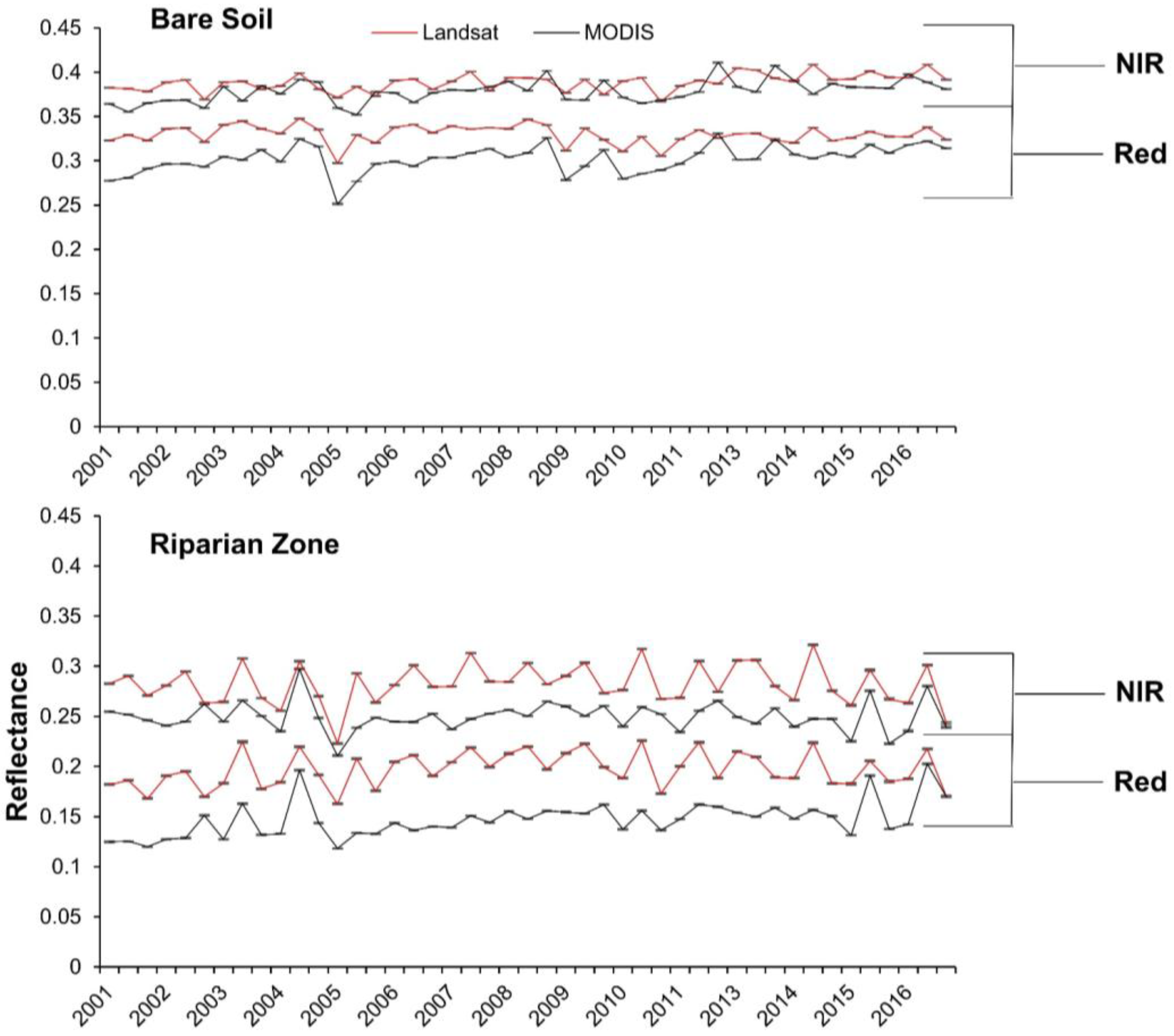
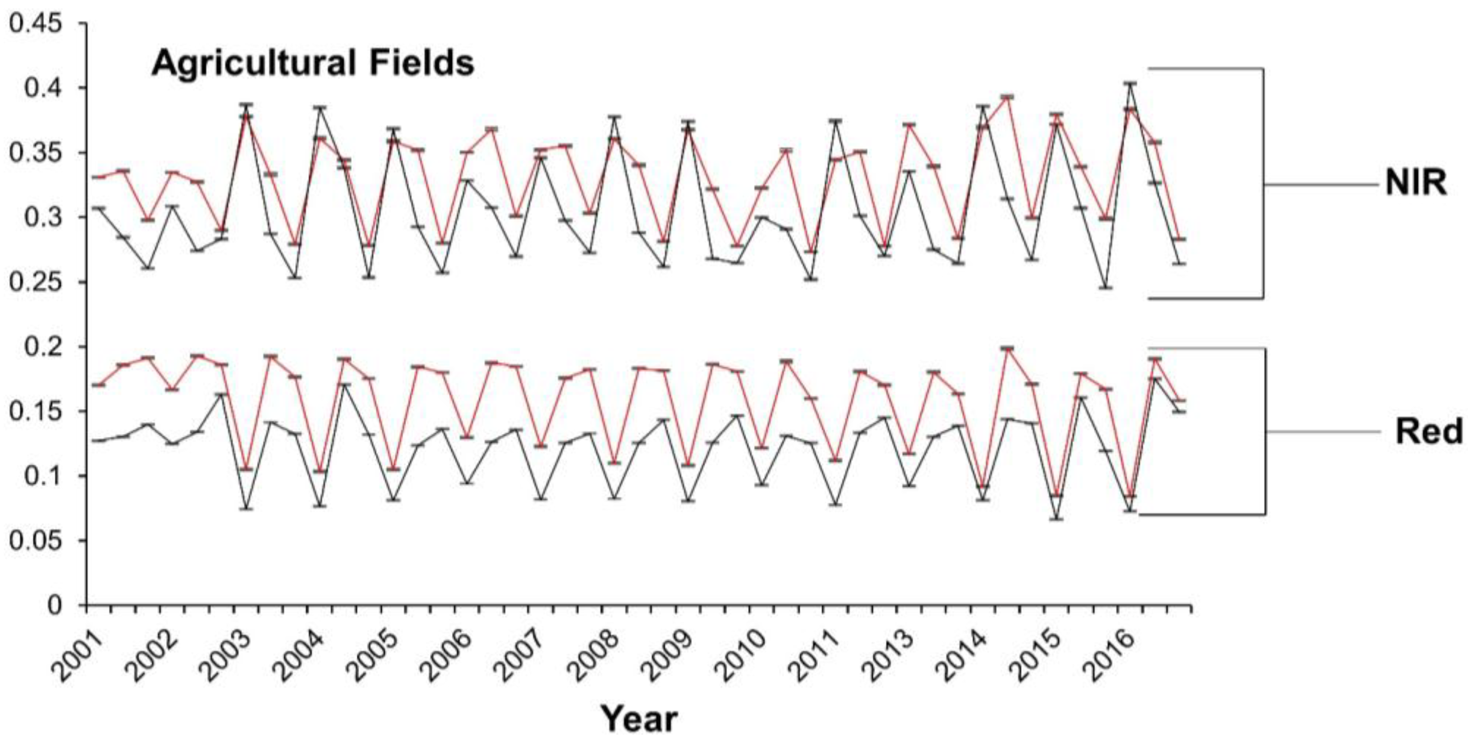
| Land Cover Type | PMRE (Red Band) | Bias (Red Band) | PMRE (NIR Band) | Bias (NIR Band) |
|---|---|---|---|---|
| Bare Soil | 9.49 | +0.03 | 3.78 | +0.01 |
| Riparian Vegetation | 34.84 | +0.05 | 13.27 | +0.03 |
| Agricultural Fields | 31.80 | +0.04 | 10.63 | +0.03 |
| Sensor | GFM | Reach 1 | Reach 2 | Reach 3 | Reach 4 | Reach 5 | Reach 6 | Reach 7 |
|---|---|---|---|---|---|---|---|---|
| Landsat 5 | R2 | 0.02 | 0.27 * | 0.49 * | 0.02 | 0.86 * | 0.83 * | 0.86 * |
| PMRE | 25.00 | 29.89 | 29.45 | 20.97 | 18.31 | 15.96 | 17.77 | |
| Bias | −0.0529 | −0.0526 | −0.0530 | −0.0506 | −0.0378 | −0.0268 | −0.0278 | |
| Landsat 8 | R2 | 0.00 | 0.24 | 0.46 * | 0.25 | 0.63 * | 0.81 * | 0.84 * |
| PMRE | 16.40 | 19.33 | 21.37 | 16.20 | 7.64 | 4.67 | 3.94 | |
| Bias | −0.0359 | −0.0331 | −0.0354 | −0.0324 | −0.0055 | +0.0039 | +0.0023 | |
| VIIRS | R2 | 0.89 * | 0.93 * | 0.97 * | 0.98 * | 0.91 * | 0.91 * | 0.96 * |
| PMRE | 14.48 | 14.19 | 15.65 | 16.07 | 20.35 | 20.19 | 22.61 | |
| Bias | +0.0244 | +0.0223 | +0.0235 | +0.0321 | +0.0347 | +0.0284 | +0.0268 |
© 2018 by the authors. Licensee MDPI, Basel, Switzerland. This article is an open access article distributed under the terms and conditions of the Creative Commons Attribution (CC BY) license (http://creativecommons.org/licenses/by/4.0/).
Share and Cite
Jarchow, C.J.; Didan, K.; Barreto-Muñoz, A.; Nagler, P.L.; Glenn, E.P. Application and Comparison of the MODIS-Derived Enhanced Vegetation Index to VIIRS, Landsat 5 TM and Landsat 8 OLI Platforms: A Case Study in the Arid Colorado River Delta, Mexico. Sensors 2018, 18, 1546. https://doi.org/10.3390/s18051546
Jarchow CJ, Didan K, Barreto-Muñoz A, Nagler PL, Glenn EP. Application and Comparison of the MODIS-Derived Enhanced Vegetation Index to VIIRS, Landsat 5 TM and Landsat 8 OLI Platforms: A Case Study in the Arid Colorado River Delta, Mexico. Sensors. 2018; 18(5):1546. https://doi.org/10.3390/s18051546
Chicago/Turabian StyleJarchow, Christopher J., Kamel Didan, Armando Barreto-Muñoz, Pamela L. Nagler, and Edward P. Glenn. 2018. "Application and Comparison of the MODIS-Derived Enhanced Vegetation Index to VIIRS, Landsat 5 TM and Landsat 8 OLI Platforms: A Case Study in the Arid Colorado River Delta, Mexico" Sensors 18, no. 5: 1546. https://doi.org/10.3390/s18051546