Analysis of a Poro-Thermo-Viscoelastic Model of Type III

Abstract

In this work, we numerically study a thermo-mechanical problem arising in poro-viscoelasticity with the type III thermal law. The thermomechanical model leads to a linear system of three coupled hyperbolic partial differential equations, and its weak formulation as three coupled parabolic linear variational equations. Then, using the finite element method and the implicit Euler scheme, for the spatial approximation and the discretization of the time derivatives, respectively, a fully discrete algorithm is introduced. A priori error estimates are proved, and the linear convergence is obtained under some suitable regularity conditions. Finally, some numerical results, involving one- and two-dimensional examples, are described, showing the accuracy of the algorithm and the dependence of the solution with respect to some constitutive parameters.

1. Introduction

Since the first works by Nunziato and Cowin [1,2], many research papers have been published involving the theory of elasticity of voids (see, for instance, [3,4,5,6,7,8,9,10,11,12,13,14,15,16,17,18,19,20] and also the monographs [21,22]). The main idea of such a theory is the assumption that the mass at each material point is found as the product of the mass density by the volume fraction, adding a new variable in the constitutive equations. This theory has become very interesting because it has been useful in applications appearing in solid mechanics (rocks, woods or even bones).

In this paper, we also consider an improvement of the classical Fourier heat law to remove the well-known paradox of infinite wave speed. It is based on the work by Green and Nagdhi [23], where the thermal displacement was included as a new independent variable into the model (even of the elastic displacement), and it is usually called type III thermal law. Since then, many authors worked on this theory (see, e.g., [4,24,25,26,27,28,29]). Here, our aim is to extend the results provided in [30], where a general thermoelastic law was studied from both mathematical (existence and uniqueness) and numerical (stability, a priori error estimates) points of view. We will consider the viscoelastic case and we will also include the porosity into the model. Therefore, using the well-known finite element method and the implicit Euler scheme, for the spatial approximation and the discretization of the time derivatives, we present a fully discrete algorithm, we perform an a priori error analysis, which leads to the linear convergence of the algorithm under some regularity conditions on the continuous solution, and we perform some numerical simulations, in one and two dimensions, to show the accuracy of the algorithm and the dependence of the solution on some constitutive parameters.

The paper is structured as follows. The thermomechanical model is described in Section 2 following [26,27,31]. Its variational formulation is also obtained and an existence and uniqueness result is stated. Then, in Section 3 a fully discrete algorithm is studied and analyzed. Finally, some numerical simulations are shown in Section 4 and some conclusions are presented in Section 5.

2. The Thermo-Mechanical Problem and Its Variational Formulation

In this section, we describe the model, the constitutive assumptions, the variational formulation of the thermomechanical problem, and we recall an existence and uniqueness result (see [26,27,31] for further details).

Denote by $\mathsf{\Omega }\subset {\mathbb{R}}^d$, $d=1,2,3$, and $[0,T]$, $T>0$, the domain occupied by the thermo-viscoelastic body and the time interval, respectively. Let also be $\mathit{x}\in \mathsf{\Omega }$ and $t\in [0,T]$ the spatial and time variables.

According to [26,27,31,32], using the linear theory of centrosymmetric isotropic and homogeneous materials, a thermo-viscoelastic body is considered. Thus, let $\mathit{u},\mathit{v}\in {\mathbb{R}}^d$ and $\phi ,e,\theta ,\psi \in \mathbb{R}$ be the displacement and velocity fields, the volume fraction, the volume fraction speed, the temperature and the thermal displacement, respectively. As usual, we have the following relations among them:

$$\mathit{u}\left(t\right)={\int }_0^t\mathit{v}\left(s\right)ds+{\mathit{u}}_0,\phi \left(t\right)={\int }_0^{t}e\left(s\right)ds+{\phi }_0,\psi \left(t\right)={\int }_0^t\theta \left(s\right)ds+{\psi }_0,$$

(1)

where ${\mathit{u}}_0$, ${\phi }_0$ and ${\psi }_0$ represent initial conditions for the displacement, the volume fraction and the thermal displacement.

Therefore, the thermomechanical problem of a centrosymmetric, isotropic and homogeneous thermo-viscoelastic body within the type III thermal theory is written as follows (see [26,27,32]).

Problem P. Find the displacement $\mathit{u}:\overline{\mathsf{\Omega }}\times [0,T]\to {\mathbb{R}}^d$, the volume fraction $\phi :\overline{\mathsf{\Omega }}\times [0,T]\to \mathbb{R}$ and the thermal displacement $\psi :\overline{\mathsf{\Omega }}\times [0,T]\to \mathbb{R}$ such that,

$$\begin{array}{c}\rho {\ddot{u}}_i={\mu }^{\ast }\mathsf{\Delta }{\dot{u}}_i+({\mu }^{\ast }+{\lambda }^{\ast }){\dot{u}}_{j,ji}+\mu \mathsf{\Delta }{u}_i+(\mu +\lambda )u_{j,ji}+\gamma {\phi }_{,i}-\beta {\dot{\psi }}_{,i}in\mathsf{\Omega }\times (0,T)fori=1,\dots ,d,\hfill \end{array}$$

(2)

$$\begin{array}{c}J\ddot{\phi }=a_0\mathsf{\Delta }\phi +\gamma u_{i,i}-\xi \phi +d\dot{\psi }+m\mathsf{\Delta }\psi in\mathsf{\Omega }\times (0,T),\hfill \end{array}$$

(3)

$$\begin{array}{c}a\ddot{\psi }=\kappa \mathsf{\Delta }\psi +m\mathsf{\Delta }\phi -d\dot{\phi }-\beta {\dot{u}}_{i,i}+{\kappa }^{\ast }\mathsf{\Delta }\dot{\psi }in\mathsf{\Omega }\times (0,T),\hfill \end{array}$$

(4)

$$\begin{array}{c}\mathit{u}=\mathbf{0},\psi =\phi =0on\partial \mathsf{\Omega }\times (0,T),\hfill \end{array}$$

(5)

$$\begin{array}{c}\mathit{u}(\mathit{x},0)={\mathit{u}}_0\left(\mathit{x}\right),\dot{\mathit{u}}(\mathit{x},0)={\mathit{v}}_0\left(\mathit{x}\right),\phi (\mathit{x},0)={\phi }_0\left(x\right)fora.e.\mathit{x}\in \mathsf{\Omega },\hfill \end{array}$$

(6)

$$\begin{array}{c}\dot{\phi }(\mathit{x},0)=e_0\left(\mathit{x}\right),\psi (\mathit{x},0)={\psi }_0\left(\mathit{x}\right),\dot{\psi }(\mathit{x},0)={\theta }_0\left(\mathit{x}\right)fora.e.\mathit{x}\in \mathsf{\Omega }.\hfill \end{array}$$

(7)

Here, ${\mathit{v}}_0,e_0$ and ${\theta }_0$ are given initial conditions for the velocity, the volume fraction speed and the temperature, respectively. As usual, the summation over repeated indexes is assumed, the partial derivative with respect to a variable is represented by a subscript preceded by a comma and one superposed dot denotes the first-order partial time derivative (two superposed dots represent the second-order partial time derivative).

In Equations (2)–(4), $\rho$ is the mass density, J is the product of the mass density by the equilibrated inertia, $\lambda$ and $\mu$ denote Lame’s coefficients, ${\lambda }^{\ast }$ and ${\mu }^{\ast }$ represent viscosity coefficients, a denotes the heat capacity, $a_0$ is the volume fraction diffusion, $\kappa$ is the thermal diffusion and ${\kappa }^{\ast }$ is the viscous thermal diffusion. The remaining coefficients $\gamma ,\beta ,\xi ,m,d$ are model parameters. We also note that, for the sake of simplicity, we have neglected in Equations (2) and (4) the respective terms corresponding to the volume forces and the heat flux.

The following assumptions are imposed on the above constitutive coefficients:

$$\begin{array}{c}\lambda >0,\mu >0,(\lambda +\mu )\xi >{\gamma }^2,a>0,\rho >0,J>0,a_0>0,{\kappa }^{\ast }>0,\hfill \\ a_0\kappa >m^2,{\mu }^{\ast }>0,{\lambda }^{\ast }+{\mu }^{\ast }>0.\hfill \end{array}$$

(8)

Now, we will derive the weak form of Problem P. Thus, denote by $Y=L^2\left(\mathsf{\Omega }\right)$, $H={\left[L^2\left(\mathsf{\Omega }\right)\right]}^d$ and $Q={\left[L^2\left(\mathsf{\Omega }\right)\right]}^{d\times d}$, and their respective scalar products (resp. norms) by ${(·,·)}_Y$, ${(·,·)}_H$ and ${(·,·)}_Q$ (resp. ${\parallel ·\parallel }_Y$, ${\parallel ·\parallel }_H$ and ${\parallel ·\parallel }_Q$). Moreover, to simplify the writing let $E=H_0^1\left(\mathsf{\Omega }\right)$ and $V={\left[H_0^1\left(\mathsf{\Omega }\right)\right]}^d$.

Using boundary conditions (5) and applying classical Green’s formula and relations (1), we obtain the weak form of Problem P as follows.

Problem VP. Find the velocity $\mathit{v}:[0,T]\to V$, the volume fraction speed $e:[0,T]\to E$ and the temperature $\theta :[0,T]\to E$ such that $\mathit{v}\left(0\right)={\mathit{v}}_0$, $e\left(0\right)=e_0$, $\theta \left(0\right)={\theta }_0$ and, for a.e. $t\in (0,T)$,

$$\begin{array}{c}\rho {(\dot{\mathit{v}}\left(t\right),\mathit{w})}_H+{\mu }^{\ast }{(\nabla \mathit{v}\left(t\right),\nabla \mathit{w})}_Q+({\lambda }^{\ast }+{\mu }^{\ast }){(\mathrm{div}\mathit{v}\left(t\right),\mathrm{div}\mathit{w})}_Y+(\lambda +\mu ){(\mathrm{div}\mathit{u}\left(t\right),\mathrm{div}\mathit{w})}_Y\hfill \\ +\mu {(\nabla \mathit{u}\left(t\right),\nabla \mathit{w})}_Q=\gamma {(\nabla \phi \left(t\right),\mathit{w})}_H-\beta {(\nabla \theta \left(t\right),\mathit{w})}_H\forall \mathit{w}\in V,\hfill \end{array}$$

(9)

$$\begin{array}{c}J{(\dot{e}\left(t\right),r)}_Y+a_0{(\nabla \phi \left(t\right),\nabla r)}_H+\xi {(\phi \left(t\right),r)}_Y+m{(\nabla \psi \left(t\right),\nabla r)}_H=d{(\theta \left(t\right),r)}_Y\hfill \\ -\gamma {(\mathrm{div}\mathit{u}\left(t\right),r)}_Y\forall r\in E,\hfill \end{array}$$

(10)

$$\begin{array}{c}a{(\dot{\theta }\left(t\right),z)}_Y+{\kappa }^{\ast }{(\nabla \theta \left(t\right),\nabla z)}_H+\kappa {(\nabla \psi \left(t\right),\nabla z)}_H+m{(\nabla \phi \left(t\right),\nabla z)}_H=-d{(e\left(t\right),z)}_Y\hfill \\ -\beta {(\mathrm{div}\mathit{v}\left(t\right),z)}_Y\forall z\in E,\hfill \end{array}$$

(11)

where the displacement, the volume fraction and the thermal displacement are then recovered from relations (1).

Proceeding as in [27,31], we can state the existence of a unique solution to Problem VP. Details are omitted for the sake of reading.

Theorem 1.

Assume that the coefficients satisfy conditions (8) and the following regularity on the initial data:

$${\mathit{u}}_0,{\mathit{v}}_0\in {\left[H^2\left(\mathsf{\Omega }\right)\right]}^d,{\phi }_0,e_0,{\psi }_0,{\theta }_0\in H^2\left(\mathsf{\Omega }\right).$$

(12)

Then, Problem VP admits a unique solution with the regularity:

$$\mathit{v}\in C([0,T];V)\cap C^1([0,T];H),e,\theta \in C([0,T];E)\cap C^1([0,T];Y).$$

3. Fully Discrete Approximations: An a Priori Error Analysis

In this section, a finite element algorithm is shown for approximating solutions to Problem VP. This is done in two steps. First, to approximate the variational spaces V and E we define the finite element spaces $V^h$ and $E^h$ as follows,

$$\begin{array}{c}{V}^h=\{{\mathit{w}}^h\in {\left[C\left(\overline{\mathsf{\Omega }}\right)\right]}^d;{\mathit{w}}_{{|}_{Tr}}^h\in {\left[P_1\left(Tr\right)\right]}^d\forall Tr\in {\mathcal{T}}^h,{\mathit{w}}^h=\mathbf{0}\mathrm{on}\partial \mathsf{\Omega }\},\hfill \end{array}$$

(13)

$$\begin{array}{c}{E}^h=\{r^h\in C\left(\overline{\mathsf{\Omega }}\right);r_{{|}_{Tr}}^h\in P_1\left(Tr\right)\forall Tr\in {\mathcal{T}}^h,r^h=0\mathrm{on}\partial \mathsf{\Omega }\},\hfill \end{array}$$

(14)

where we assume that $\mathsf{\Omega }$ is a polyhedral domain and we denote by ${\mathcal{T}}^h$ a regular triangulation of $\overline{\mathsf{\Omega }}$. Moreover, the space of polynomials of global degree less or equal to 1 in element $Tr$ is represented by $P_1\left(Tr\right)$. Here, $h>0$ denotes the spatial discretization parameter.

Secondly, in order to discretize the time derivatives we use a uniform partition of the time interval $[0,T]$, that we denote by $0=t_0<t_1<\dots <t_N=T$ ($k=T/N$ is the time step size). Moreover, for a continuous function $f\left(t\right)$ we denote $f_n=f\left(t_n\right)$ and, for the sequence ${\left\{z_n\right\}}_{n=0}^N$, let $\delta z_n=(z_n-z_{n-1})/k$ be its corresponding divided differences.

Using the classical implicit Euler scheme, the fully discrete approximation of Problem VP is the following.

Problem VP${}^{\mathit{hk}}$.Find the discrete velocity ${\mathit{v}}^{hk}={\left\{{\mathit{v}}_n^{hk}\right\}}_{n=0}^N\subset V^h$, the discrete volume fraction speed $e^{hk}={\left\{e_n^{hk}\right\}}_{n=0}^N\subset E^h$ and the discrete temperature ${\theta }^{hk}={\left\{{\theta }_n^{hk}\right\}}_{n=0}^N\subset E^h$ such that ${\mathit{v}}_0^{hk}={\mathit{v}}_0^h$, $e_0^{hk}=e_0^h$, ${\theta }_0^{hk}={\theta }_0^h$, and, for $n=1,\dots ,N$,

$$\begin{array}{c}\rho {(\delta {\mathit{v}}_n^{hk},{\mathit{w}}^h)}_H+{\mu }^{\ast }{(\nabla {\mathit{v}}_n^{hk},\nabla {\mathit{w}}^h)}_Q+({\lambda }^{\ast }+{\mu }^{\ast }){(\mathrm{div}{\mathit{v}}_n^{hk},\mathrm{div}{\mathit{w}}^h)}_Y+(\lambda +\mu ){(\mathrm{div}{\mathit{u}}_n^{hk},\mathrm{div}{\mathit{w}}^h)}_Y\hfill \\ +\mu {(\nabla {\mathit{u}}_n^{hk},\nabla {\mathit{w}}^h)}_Q=\gamma {(\nabla {\phi }_n^{hk},{\mathit{w}}^h)}_H-\beta {(\nabla {\theta }_n^{hk},{\mathit{w}}^h)}_H\forall {\mathit{w}}^h\in V^h,\hfill \end{array}$$

(15)

$$\begin{array}{c}J{(\delta e_n^{hk},r^h)}_Y+a_0{(\nabla {\phi }_n^{hk},\nabla r^h)}_H+\xi {({\phi }_n^{hk},r^h)}_Y+m{(\nabla {\psi }_n^{hk},\nabla r^h)}_H=d{({\theta }_n^{hk},r^h)}_Y\hfill \\ -\gamma {(\mathrm{div}{\mathit{u}}_n^{hk},r^h)}_Y\forall r^h\in E^h,\hfill \end{array}$$

(16)

$$\begin{array}{c}a{(\delta {\theta }_n^{hk},z^h)}_Y+{\kappa }^{\ast }{(\nabla {\theta }_n^{hk},\nabla z^h)}_H+\kappa {(\nabla {\psi }_n^{hk},\nabla z^h)}_H+m{(\nabla {\phi }_n^{hk},\nabla z^h)}_H=-d{(e_n^{hk},z^h)}_Y\hfill \\ -\beta {(\mathrm{div}{\mathit{v}}_n^{hk},z^h)}_Y\forall z^h\in E^h,\hfill \end{array}$$

(17)

where the discrete displacement, the discrete volume fraction and the discrete thermal displacement are then recovered from the relations:

$${\mathit{u}}_n^{hk}=k\sum _{j=1}^n{\mathit{v}}_j^{hk}+{\mathit{u}}_0^h,{\phi }_n^{hk}=k\sum _{j=1}^n{e}_j^{hk}+{\phi }_0^h,{\psi }_n^{hk}=k\sum _{j=1}^n{\theta }_j^{hk}+{\psi }_0^h,$$

(18)

and the discrete initial conditions, denoted by ${\mathit{u}}_0^h$, ${\mathit{v}}_0^h$, ${\phi }_0^h$, $e_0^h$, ${\psi }_0^h$ and ${\theta }_0^h$ are given by

$${\mathit{u}}_0^h={\mathcal{P}}^{1h}{\mathit{u}}_0,{\mathit{v}}_0^h={\mathcal{P}}^{1h}{\mathit{v}}_0,{\phi }_0^h={\mathcal{P}}^{2h}{\phi }_0,e_0^h={\mathcal{P}}^{2h}{e}_0,{\psi }_0^h={\mathcal{P}}^{2h}{\psi }_0,{\theta }_0^h={\mathcal{P}}^{2h}{\theta }_0.$$

(19)

Here, ${\mathcal{P}}^{1h}$ and ${\mathcal{P}}^{2h}$ are the respective projection operators over the finite element spaces $V^h$ and $E^h$ (see [33]).

It is easy to show that discrete problem VP${}^{hk}$ admits a unique solution using well-known results on linear variational equations and conditions (8), so we omit the details.

The aim of this section is to obtain some a priori error estimates on the numerical errors ${\mathit{u}}_n-{\mathit{u}}_n^{hk}$, ${\mathit{v}}_n-{\mathit{v}}_n^{hk}$, ${\phi }_n-{\phi }_n^{hk}$, $e_n-e_n^{hk}$, ${\psi }_n-{\psi }_n^{hk}$ and ${\theta }_n-{\theta }_n^{hk}$.

First, we obtain the estimates on the velocity field. Subtracting Equation (9) at time $t=t_n$ for a test function $\mathit{w}={\mathit{w}}^h\in V^h\subset V$ and discrete Equation (15), we have, for all ${\mathit{w}}^h\in V^h$,

$$\begin{array}{c}{\displaystyle \rho {({\dot{\mathit{v}}}_n-\delta {\mathit{v}}_n^{hk},{\mathit{w}}^h)}_H+{\mu }^{\ast }{(\nabla ({\mathit{v}}_n-{\mathit{v}}_n^{hk}),\nabla {\mathit{w}}^h)}_Q+({\lambda }^{\ast }+{\mu }^{\ast }){(\mathrm{div}({\mathit{v}}_n-{\mathit{v}}_n^{hk}),\mathrm{div}{\mathit{w}}^h)}_Y}\hfill \\ +(\lambda +\mu ){(\mathrm{div}({\mathit{u}}_n-{\mathit{u}}_n^{hk}),\mathrm{div}{\mathit{w}}^h)}_Y+\mu {(\nabla ({\mathit{u}}_n-{\mathit{u}}_n^{hk}),\nabla {\mathit{w}}^h)}_Q-\gamma {(\nabla ({\phi }_n-{\phi }_n^{hk}),{\mathit{w}}^h)}_H\hfill \\ +\beta {(\nabla ({\theta }_n-{\theta }_n^{hk}),{\mathit{w}}^h)}_H=0,\hfill \end{array}$$

and so,

$$\begin{array}{c}{\displaystyle \rho {({\dot{\mathit{v}}}_n-\delta {\mathit{v}}_n^{hk},{\mathit{v}}_n-{\mathit{v}}_n^{hk})}_H+{\mu }^{\ast }{(\nabla ({\mathit{v}}_n-{\mathit{v}}_n^{hk}),\nabla ({\mathit{v}}_n-{\mathit{v}}_n^{hk}))}_Q+\mu {(\nabla ({\mathit{u}}_n-{\mathit{u}}_n^{hk}),\nabla ({\mathit{v}}_n-{\mathit{v}}_n^{hk}))}_Q}\hfill \\ +({\lambda }^{\ast }+{\mu }^{\ast }){(\mathrm{div}({\mathit{v}}_n-{\mathit{v}}_n^{hk}),\mathrm{div}({\mathit{v}}_n-{\mathit{v}}_n^{hk}))}_Y+(\lambda +\mu ){(\mathrm{div}({\mathit{u}}_n-{\mathit{u}}_n^{hk}),\mathrm{div}({\mathit{v}}_n-{\mathit{v}}_n^{hk}))}_Y\hfill \\ -\gamma {(\nabla ({\phi }_n-{\phi }_n^{hk}),{\mathit{v}}_n-{\mathit{v}}_n^{hk})}_H+\beta {(\nabla ({\theta }_n-{\theta }_n^{hk}),{\mathit{v}}_n-{\mathit{v}}_n^{hk})}_H\hfill \\ {\displaystyle =\rho {({\dot{\mathit{v}}}_n-\delta {\mathit{v}}_n^{hk},{\mathit{v}}_n-{\mathit{w}}^h)}_H+{\mu }^{\ast }{(\nabla ({\mathit{v}}_n-{\mathit{v}}_n^{hk}),\nabla ({\mathit{v}}_n-{\mathit{w}}^h))}_Q+\mu {(\nabla ({\mathit{u}}_n-{\mathit{u}}_n^{hk}),\nabla ({\mathit{v}}_n-{\mathit{w}}^h))}_Q}\hfill \\ +({\lambda }^{\ast }+{\mu }^{\ast }){(\mathrm{div}({\mathit{v}}_n-{\mathit{v}}_n^{hk}),\mathrm{div}({\mathit{v}}_n-{\mathit{w}}^h))}_Y+(\lambda +\mu ){(\mathrm{div}({\mathit{u}}_n-{\mathit{u}}_n^{hk}),\mathrm{div}({\mathit{v}}_n-{\mathit{w}}^h))}_Y\hfill \\ -\gamma {(\nabla ({\phi }_n-{\phi }_n^{hk}),{\mathit{v}}_n-{\mathit{w}}^h)}_H+\beta {(\nabla ({\theta }_n-{\theta }_n^{hk}),{\mathit{v}}_n-{\mathit{w}}^h)}_H\forall {\mathit{w}}^h\in V^h.\hfill \end{array}$$

It is straightforward to show that

$$\begin{array}{c}{\displaystyle {({\dot{\mathit{v}}}_n-\delta {\mathit{v}}_n^{hk},{\mathit{v}}_n-{\mathit{v}}_n^{hk})}_H\ge {({\dot{\mathit{v}}}_n-\delta {\mathit{v}}_n,{\mathit{v}}_n-{\mathit{v}}_n^{hk})}_H}\hfill \\ {\displaystyle +\frac{1}{2k}\left[\parallel {\mathit{v}}_n-{\mathit{v}}_n^{hk}{\parallel }_H^2-{\parallel {\mathit{v}}_{n-1}-{\mathit{v}}_{n-1}^{hk}\parallel }_H^2\right],}\hfill \\ {\displaystyle {(\nabla ({\mathit{u}}_n-{\mathit{u}}_n^{hk}),\nabla ({\mathit{v}}_n-{\mathit{v}}_n^{hk}))}_Q\ge {(\nabla ({\mathit{u}}_n-{\mathit{u}}_n^{hk}),\nabla ({\dot{\mathit{u}}}_n-\delta {\mathit{u}}_n))}_Q}\hfill \\ {\displaystyle +\frac{1}{2k}\left[\parallel \nabla ({\mathit{u}}_n-{\mathit{u}}_n^{hk}){\parallel }_Q^2-{\parallel \nabla ({\mathit{u}}_{n-1}-{\mathit{u}}_{n-1}^{hk})\parallel }_Q^2\right],}\hfill \\ {\displaystyle {(\mathrm{div}({\mathit{u}}_n-{\mathit{u}}_n^{hk}),\mathrm{div}({\mathit{v}}_n-{\mathit{v}}_n^{hk}))}_Y={(\mathrm{div}({\mathit{u}}_n-{\mathit{u}}_n^{hk}),\mathrm{div}({\dot{\mathit{u}}}_n-\delta {\mathit{u}}_n))}_Y}\hfill \\ {\displaystyle +\frac{1}{2k}[\parallel \mathrm{div}({\mathit{u}}_n-{\mathit{u}}_n^{hk}){\parallel }_Y^2-{\parallel \mathrm{div}({\mathit{u}}_{n-1}-{\mathit{u}}_{n-1}^{hk})\parallel }_Y^2}\hfill \\ {\displaystyle +\parallel \mathrm{div}({\mathit{u}}_n-{\mathit{u}}_n^{hk}-({\mathit{u}}_{n-1}-{\mathit{u}}_{n-1}^{hk})){\parallel }_Y^2],}\hfill \\ {(\nabla ({\theta }_n-{\theta }_n^{hk}),{\mathit{v}}_n-{\mathit{w}}^h)}_H=-{({\theta }_n-{\theta }_n^{hk},\mathrm{div}({\mathit{v}}_n-{\mathit{w}}^h))}_Y,\hfill \\ {(\nabla ({\phi }_n-{\phi }_n^{hk}),{\mathit{v}}_n-{\mathit{w}}^h)}_H=-{({\phi }_n-{\phi }_n^{hk},\mathrm{div}({\mathit{v}}_n-{\mathit{w}}^h))}_Y,\hfill \\ {(\nabla ({\theta }_n-{\theta }_n^{hk}),{\mathit{v}}_n-{\mathit{v}}_n^{hk})}_H=-{({\theta }_n-{\theta }_n^{hk},\mathrm{div}({\mathit{v}}_n-{\mathit{v}}_n^{hk}))}_Y,\hfill \\ {(\nabla ({\phi }_n-{\phi }_n^{hk}),{\mathit{v}}_n-{\mathit{v}}_n^{hk})}_H=-{({\phi }_n-{\phi }_n^{hk},\mathrm{div}({\mathit{v}}_n-{\mathit{v}}_n^{hk}))}_Y,\hfill \end{array}$$

where we have used that ${\mathit{v}}_n^{hk}=\delta {\mathit{u}}_n^{hk}=({\mathit{u}}_n^{hk}-{\mathit{u}}_{n-1}^{hk})/k$ and notations $\delta {\mathit{v}}_n=({\mathit{v}}_n-{\mathit{v}}_{n-1})/k$ and $\delta {\mathit{u}}_n=({\mathit{u}}_n-{\mathit{u}}_{n-1})/k$. Therefore, we find that, for all ${\mathit{w}}^h\in V^h$,

$$\begin{array}{c}{\displaystyle \frac{\rho }{2k}\left[\parallel {\mathit{v}}_n-{\mathit{v}}_n^{hk}{\parallel }_H^2-{\parallel {\mathit{v}}_{n-1}-{\mathit{v}}_{n-1}^{hk}\parallel }_H^2\right]+C\parallel \nabla ({\mathit{v}}_n-{\mathit{v}}_n^{hk}){\parallel }_Q^2+C{\parallel \mathrm{div}({\mathit{v}}_n-{\mathit{v}}_n^{hk})\parallel }_Y^2}\hfill \\ {\displaystyle +\frac{\mu }{2k}\left[\parallel \nabla ({\mathit{u}}_n-{\mathit{u}}_n^{hk}){\parallel }_Q^2-{\parallel \nabla ({\mathit{u}}_{n-1}-{\mathit{u}}_{n-1}^{hk})\parallel }_Q^2\right]+\beta {({\theta }_n-{\theta }_n^{hk},\mathrm{div}({\mathit{v}}_n-{\mathit{v}}_n^{hk}))}_Y}\hfill \\ +\frac{\lambda +\mu }{2k}[\parallel \mathrm{div}({\mathit{u}}_n-{\mathit{u}}_n^{hk}){\parallel }_Y^2-{\parallel \mathrm{div}({\mathit{u}}_{n-1}-{\mathit{u}}_{n-1}^{hk})\parallel }_Y^2\hfill \\ +\parallel \mathrm{div}({\mathit{u}}_n-{\mathit{u}}_n^{hk}-({\mathit{u}}_{n-1}-{\mathit{u}}_{n-1}^{hk})){\parallel }_Y^2]+\gamma {({\phi }_n-{\phi }_n^{hk},\mathrm{div}({\mathit{v}}_n-{\mathit{v}}_n^{hk}))}_Y\hfill \\ \le C(\parallel {\mathit{v}}_n-{\mathit{v}}_n^{hk}{\parallel }_H^2+\parallel {\dot{\mathit{v}}}_n-\delta {\mathit{v}}_n{\parallel }_H^2+\parallel \nabla ({\mathit{u}}_n-{\mathit{u}}_n^{hk}){\parallel }_Q^2+{\parallel \mathrm{div}({\mathit{u}}_n-{\mathit{u}}_n^{hk})\parallel }_Y^2\hfill \\ +\parallel {\mathit{v}}_n-{\mathit{w}}^h{\parallel }_H^2+\parallel \nabla ({\mathit{v}}_n-{\mathit{w}}^h){\parallel }_Q^2+\parallel \mathrm{div}({\mathit{v}}_n-{\mathit{w}}^h){\parallel }_Y^2+{\parallel {\phi }_n-{\phi }_n^{hk}\parallel }_Y^2\hfill \\ +\parallel \nabla ({\dot{\mathit{u}}}_n-\delta {\mathit{u}}_n){\parallel }_Q^2+{\parallel \mathrm{div}({\dot{\mathit{u}}}_n-\delta {\mathit{u}}_n)\parallel }_Y^2+{(\delta {\mathit{v}}_n-\delta {\mathit{v}}_n^{hk},{\mathit{v}}_n-{\mathit{w}}^h)}_H\hfill \\ +\parallel {\theta }_n-{\theta }_n^{hk}{\parallel }_Y^2).\hfill \end{array}$$

(20)

Here and in what follows, $C>0$ denotes a positive constant whose value may change for each expression, which depends on the continuous solution but it is independent of the discretization parameters h and k.

Secondly, we will find the error estimates on the volume fraction speed. Then, we subtract Equation (10) at time $t=t_n$ for a test function $r=r^h\in E^h\subset E$ and discrete Equation (16) to obtain, for all $r^h\in E^h$,

$$\begin{array}{c}{\displaystyle J{({\dot{e}}_n-\delta e_n^{hk},r^h)}_Y+a_0{(\nabla ({\phi }_n-{\phi }_n^{hk}),\nabla r^h)}_H+\xi {({\phi }_n-{\phi }_n^{hk},r^h)}_Y+m{(\nabla ({\psi }_n-{\psi }_n^{hk}),\nabla r^h)}_H}\hfill \\ =d{({\theta }_n-{\theta }_n^{hk},r^h)}_Y-\gamma {(\mathrm{div}({\mathit{u}}_n-{\mathit{u}}_n^{hk}),r^h)}_Y.\hfill \end{array}$$

Thus, we find, for all $r^h\in E^h$,

$$\begin{array}{c}{\displaystyle J{({\dot{e}}_n-\delta e_n^{hk},e_n-e_n^{hk})}_Y+a_0{(\nabla ({\phi }_n-{\phi }_n^{hk}),\nabla (e_n-e_n^{hk}))}_H+\xi {({\phi }_n-{\phi }_n^{hk},e_n-e_n^{hk})}_Y}\hfill \\ +m{(\nabla ({\psi }_n-{\psi }_n^{hk}),\nabla (e_n-e_n^{hk}))}_H-d{({\theta }_n-{\theta }_n^{hk},e_n-e_n^{hk})}_Y+\gamma {(\mathrm{div}({\mathit{u}}_n-{\mathit{u}}_n^{hk}),e_n-e_n^{hk})}_Y\hfill \\ {\displaystyle =J{({\dot{e}}_n-\delta e_n^{hk},e_n-r^h)}_Y+a_0{(\nabla ({\phi }_n-{\phi }_n^{hk}),\nabla (e_n-r^h))}_H+\xi {({\phi }_n-{\phi }_n^{hk},e_n-r^h)}_Y}\hfill \\ +m{(\nabla ({\psi }_n-{\psi }_n^{hk}),\nabla (e_n-r^h))}_H-d{({\theta }_n-{\theta }_n^{hk},e_n-r^h)}_Y+\gamma {(\mathrm{div}({\mathit{u}}_n-{\mathit{u}}_n^{hk}),e_n-r^h)}_Y.\hfill \end{array}$$

Since

$$\begin{array}{c}{\displaystyle {({\dot{e}}_n-\delta e_n^{hk},e_n-e_n^{hk})}_Y\ge {({\dot{e}}_n-\delta e_n,e_n-e_n^{hk})}_Y+\frac{1}{2k}\left[\parallel e_n-e_n^{hk}{\parallel }_Y^2-{\parallel e_{n-1}-e_{n-1}^{hk}\parallel }_Y^2\right],}\hfill \\ {\displaystyle {(\nabla ({\phi }_n-{\phi }_n^{hk}),\nabla (e_n-e_n^{hk}))}_H={(\nabla ({\phi }_n-{\phi }_n^{hk}),\nabla ({\dot{\phi }}_n-\delta {\phi }_n))}_H}\hfill \\ {\displaystyle +\frac{1}{2k}\left[\parallel \nabla ({\phi }_n-{\phi }_n^{hk}){\parallel }_H^2-\parallel \nabla ({\phi }_{n-1}-{\phi }_{n-1}^{hk}){{\parallel }_H^2+\nabla ({\phi }_n-{\phi }_n^{hk}-({\phi }_{n-1}-{\phi }_{n-1}^{hk}))\parallel }_H^2\right],}\hfill \\ {\displaystyle {({\phi }_n-{\phi }_n^{hk},e_n-e_n^{hk})}_Y={({\phi }_n-{\phi }_n^{hk},{\dot{\phi }}_n-\delta {\phi }_n)}_Y+\frac{1}{2k}[\parallel {\phi }_n-{\phi }_n^{hk}{\parallel }_Y^2-{\parallel {\phi }_{n-1}-{\phi }_{n-1}^{hk}\parallel }_Y^2}\hfill \\ {\displaystyle +\parallel {\phi }_n-{\phi }_n^{hk}-({\phi }_{n-1}-{\phi }_{n-1}^{hk}){\parallel }_Y^2],}\hfill \end{array}$$

where we have used the fact that $e_n^{hk}=\delta {\phi }_n^{hk}=({\phi }_n^{hk}-{\phi }_{n-1}^{hk})/k$ and the notations $\delta e_n=(e_n-e_{n-1})/k$ and $\delta {\phi }_n=({\phi }_n-{\phi }_{n-1})/k$, it follows that, for all $r^h\in E^h$,

$$\begin{array}{c}{\displaystyle \frac{J}{2k}\left[\parallel e_n-e_n^{hk}{\parallel }_Y^2-{\parallel e_{n-1}-e_{n-1}^{hk}\parallel }_Y^2\right]}\hfill \\ +\frac{a_0}{2k}\left[\parallel \nabla ({\phi }_n-{\phi }_n^{hk}){\parallel }_H^2-\parallel \nabla ({\phi }_{n-1}-{\phi }_{n-1}^{hk}){{\parallel }_H^2+\nabla ({\phi }_n-{\phi }_n^{hk}-({\phi }_{n-1}-{\phi }_{n-1}^{hk}))\parallel }_H^2\right]\hfill \\ +\frac{\xi }{2k}\left[\parallel {\phi }_n-{\phi }_n^{hk}{\parallel }_Y^2-\parallel {\phi }_{n-1}-{\phi }_{n-1}^{hk}{\parallel }_Y^2+{\parallel {\phi }_n-{\phi }_n^{hk}-({\phi }_{n-1}-{\phi }_{n-1}^{hk})\parallel }_Y^2\right]\hfill \\ +m{(\nabla ({\psi }_n-{\psi }_n^{hk}),\nabla (e_n-e_n^{hk}))}_H-d{({\theta }_n-{\theta }_n^{hk},e_n-e_n^{hk})}_Y+\gamma {(\mathrm{div}({\mathit{u}}_n-{\mathit{u}}_n^{hk}),e_n-e_n^{hk})}_Y\hfill \\ \le C(\parallel e_n-e_n^{hk}{\parallel }_Y^2+\parallel {\dot{e}}_n-\delta e_n{\parallel }_Y^2+\parallel \nabla ({\phi }_n-{\phi }_n^{hk}){\parallel }_H^2+\parallel {\phi }_n-{\phi }_n^{hk}{\parallel }_Y^2+{\parallel e_n-r^h\parallel }_Y^2\hfill \\ +\parallel \nabla (e_n-r^h){\parallel }_H^2+\parallel \nabla ({\dot{\phi }}_n-\delta {\phi }_n){\parallel }_H^2+{\parallel {\dot{\phi }}_n-\delta {\phi }_n\parallel }_Y^2+{(\delta e_n-\delta e_n^{hk},e_n-r^h)}_Y\hfill \\ +\parallel {\theta }_n-{\theta }_n^{hk}{\parallel }_Y^2+{\parallel \mathrm{div}({\mathit{u}}_n-{\mathit{u}}_n^{hk})\parallel }_Y^2).\hfill \end{array}$$

(21)

Finally, we get the estimates on the temperature field. Then, we subtract Equation (11) at time $t=t_n$ for a test function $z=z^h\in E^h\subset E$ and discrete Equation (17) to have, for all $z^h\in E^h$,

$$\begin{array}{c}a{({\dot{\theta }}_n-\delta {\theta }_n^{hk},z^h)}_Y+{\kappa }^{\ast }{(\nabla ({\theta }_n-{\theta }_n^{hk}),\nabla z^h)}_H+\kappa {(\nabla ({\psi }_n-{\psi }_n^{hk}),\nabla z^h)}_H+m{(\nabla ({\phi }_n-{\phi }_n^{hk}),\nabla z^h)}_H\hfill \\ +d{(e_n-e_n^{hk},z^h)}_Y+\beta {(\mathrm{div}({\mathit{v}}_n-{\mathit{v}}_n^{hk}),z^h)}_Y=0,\hfill \end{array}$$

and so, it follows that, for all $z^h\in E^h$,

$$\begin{array}{c}a{({\dot{\theta }}_n-\delta {\theta }_n^{hk},{\theta }_n-{\theta }_n^{hk})}_Y+{\kappa }^{\ast }{(\nabla ({\theta }_n-{\theta }_n^{hk}),\nabla ({\theta }_n-{\theta }_n^{hk}))}_H+\kappa {(\nabla ({\psi }_n-{\psi }_n^{hk}),\nabla ({\theta }_n-{\theta }_n^{hk}))}_H\hfill \\ +m{(\nabla ({\phi }_n-{\phi }_n^{hk}),\nabla ({\theta }_n-{\theta }_n^{hk}))}_H+d{(e_n-e_n^{hk},{\theta }_n-{\theta }_n^{hk})}_Y+\beta {(\mathrm{div}({\mathit{v}}_n-{\mathit{v}}_n^{hk}),{\theta }_n-{\theta }_n^{hk})}_Y\hfill \\ =a{({\dot{\theta }}_n-\delta {\theta }_n^{hk},{\theta }_n-z^h)}_Y+{\kappa }^{\ast }{(\nabla ({\theta }_n-{\theta }_n^{hk}),\nabla ({\theta }_n-z^h))}_H+\kappa {(\nabla ({\psi }_n-{\psi }_n^{hk}),\nabla ({\theta }_n-z^h))}_H\hfill \\ +m{(\nabla ({\phi }_n-{\phi }_n^{hk}),\nabla ({\theta }_n-z^h))}_H+d{(e_n-e_n^{hk},{\theta }_n-z^h)}_Y+\beta {(\mathrm{div}({\mathit{v}}_n-{\mathit{v}}_n^{hk}),{\theta }_n-z^h)}_Y.\hfill \end{array}$$

Keeping in mind that

$$\begin{array}{c}{\displaystyle {({\dot{\theta }}_n-\delta {\theta }_n^{hk},{\theta }_n-{\theta }_n^{hk})}_Y\ge {({\dot{\theta }}_n-\delta {\theta }_n,{\theta }_n-{\theta }_n^{hk})}_Y+\frac{1}{2k}\left[\parallel {\theta }_n-{\theta }_n^{hk}{\parallel }_Y^2-{\parallel {\theta }_{n-1}-{\theta }_{n-1}^{hk}\parallel }_Y^2\right],}\hfill \\ {\displaystyle {(\nabla ({\psi }_n-{\psi }_n^{hk}),\nabla ({\theta }_n-{\theta }_n^{hk}))}_H={(\nabla ({\psi }_n-{\psi }_n^{hk}),\nabla ({\dot{\psi }}_n-\delta {\psi }_n))}_H}\hfill \\ {\displaystyle +\frac{1}{2k}\left[\parallel \nabla ({\psi }_n-{\psi }_n^{hk}){\parallel }_H^2-\parallel \nabla ({\psi }_{n-1}-{\psi }_{n-1}^{hk}){\parallel }_H^2+{\parallel \nabla ({\psi }_n-{\psi }_n^{hk}-({\psi }_{n-1}-{\psi }_{n-1}^{hk}))\parallel }_H^2\right],}\hfill \\ {\displaystyle {(\mathrm{div}({\mathit{v}}_n-{\mathit{v}}_n^{hk}),{\theta }_n-z^h)}_Y=-{({\mathit{v}}_n-{\mathit{v}}_n^{hk},\nabla ({\theta }_n-z^h))}_H,}\hfill \end{array}$$

where we have used the fact that ${\theta }_n^{hk}=\delta {\psi }_n^{hk}=({\psi }_n^{hk}-{\psi }_{n-1}^{hk})/k$ and the notations $\delta {\theta }_n=({\theta }_n-{\theta }_{n-1})/k$ and $\delta {\psi }_n=({\psi }_n-{\psi }_{n-1})/k$, we obtain, for all $z^h\in E^h$,

$$\begin{array}{c}{\displaystyle \frac{a}{2k}\left[\parallel {\theta }_n-{\theta }_n^{hk}{\parallel }_Y^2-{\parallel {\theta }_{n-1}-{\theta }_{n-1}^{hk}\parallel }_Y^2\right]+C{\parallel \nabla ({\theta }_n-{\theta }_n^{hk})\parallel }_H^2}\hfill \\ {\displaystyle +\frac{\kappa }{2k}\left[\parallel \nabla ({\psi }_n-{\psi }_n^{hk}){\parallel }_H^2-\parallel \nabla ({\psi }_{n-1}-{\psi }_{n-1}^{hk}){\parallel }_H^2+{\parallel \nabla ({\psi }_n-{\psi }_n^{hk}-({\psi }_{n-1}-{\psi }_{n-1}^{hk}))\parallel }_H^2\right]}\hfill \\ +m{(\nabla ({\phi }_n-{\phi }_n^{hk}),\nabla ({\theta }_n-{\theta }_n^{hk}))}_H+d{(e_n-e_n^{hk},{\theta }_n-{\theta }_n^{hk})}_Y+\beta {(\mathrm{div}({\mathit{v}}_n-{\mathit{v}}_n^{hk}),{\theta }_n-{\theta }_n^{hk})}_Y\hfill \\ \le C(\parallel {\theta }_n-{\theta }_n^{hk}{\parallel }_Y^2+\parallel {\dot{\theta }}_n-\delta {\theta }_n{\parallel }_Y^2+\parallel \nabla ({\psi }_n-{\psi }_n^{hk}){\parallel }_H^2+\parallel {\theta }_n-z^h{\parallel }_Y^2+{\parallel \nabla ({\theta }_n-z^h)\parallel }_H^2\hfill \\ +\parallel {\mathit{v}}_n-{\mathit{v}}_n^{hk}{\parallel }_H^2+\parallel e_n-e_n^{hk}{\parallel }_Y^2+{(\delta {\theta }_n-\delta {\theta }_n^{hk},{\theta }_n-z^h)}_Y+{\parallel \nabla ({\dot{\psi }}_n-\delta {\psi }_n)\parallel }_H^2\hfill \\ +\parallel \nabla ({\phi }_n-{\phi }_n^{hk}){\parallel }_H^2).\hfill \end{array}$$

(22)

Combining now estimates (20)–(22) we find that

$$\begin{array}{c}{\displaystyle \frac{\rho }{2k}\left[\parallel {\mathit{v}}_n-{\mathit{v}}_n^{hk}{\parallel }_H^2-{\parallel {\mathit{v}}_{n-1}-{\mathit{v}}_{n-1}^{hk}\parallel }_H^2\right]+C\parallel \nabla ({\mathit{v}}_n-{\mathit{v}}_n^{hk}){\parallel }_Q^2+C{\parallel \mathrm{div}({\mathit{v}}_n-{\mathit{v}}_n^{hk})\parallel }_Y^2}\hfill \\ {\displaystyle +\frac{\mu }{2k}\left[\parallel \nabla ({\mathit{u}}_n-{\mathit{u}}_n^{hk}){\parallel }_Q^2-{\parallel \nabla ({\mathit{u}}_{n-1}-{\mathit{u}}_{n-1}^{hk})\parallel }_Q^2\right]}\hfill \\ +\frac{\lambda +\mu }{2k}[\parallel \mathrm{div}({\mathit{u}}_n-{\mathit{u}}_n^{hk}){\parallel }_Y^2-{\parallel \mathrm{div}({\mathit{u}}_{n-1}-{\mathit{u}}_{n-1}^{hk})\parallel }_Y^2\hfill \\ +\parallel \mathrm{div}({\mathit{u}}_n-{\mathit{u}}_n^{hk}-({\mathit{u}}_{n-1}-{\mathit{u}}_{n-1}^{hk})){\parallel }_Y^2]+\gamma {({\phi }_n-{\phi }_n^{hk},\mathrm{div}({\mathit{v}}_n-{\mathit{v}}_n^{hk}))}_Y\hfill \\ {\displaystyle +\frac{J}{2k}\left[\parallel e_n-e_n^{hk}{\parallel }_Y^2-{\parallel e_{n-1}-e_{n-1}^{hk}\parallel }_Y^2\right]+m{(\nabla ({\phi }_n-{\phi }_n^{hk}),\nabla ({\theta }_n-{\theta }_n^{hk}))}_H}\hfill \\ +\frac{\xi }{2k}\left[\parallel {\phi }_n-{\phi }_n^{hk}{\parallel }_Y^2-\parallel {\phi }_{n-1}-{\phi }_{n-1}^{hk}{\parallel }_Y^2+{\parallel {\phi }_n-{\phi }_n^{hk}-({\phi }_{n-1}-{\phi }_{n-1}^{hk})\parallel }_Y^2\right]\hfill \\ +m{(\nabla ({\psi }_n-{\psi }_n^{hk}),\nabla (e_n-e_n^{hk}))}_H+\gamma {(\mathrm{div}({\mathit{u}}_n-{\mathit{u}}_n^{hk}),e_n-e_n^{hk})}_Y\hfill \\ {\displaystyle +\frac{a}{2k}\left[\parallel {\theta }_n-{\theta }_n^{hk}{\parallel }_Y^2-{\parallel {\theta }_{n-1}-{\theta }_{n-1}^{hk}\parallel }_Y^2\right]+C{\parallel \nabla ({\theta }_n-{\theta }_n^{hk})\parallel }_H^2}\hfill \\ {\displaystyle +\frac{\kappa }{2k}\left[\parallel \nabla ({\psi }_n-{\psi }_n^{hk}){\parallel }_H^2-\parallel \nabla ({\psi }_{n-1}-{\psi }_{n-1}^{hk}){\parallel }_H^2+{\parallel \nabla ({\psi }_n-{\psi }_n^{hk}-({\psi }_{n-1}-{\psi }_{n-1}^{hk}))\parallel }_H^2\right]}\hfill \\ +\frac{a_0}{2k}\left[\parallel \nabla ({\phi }_n-{\phi }_n^{hk}){\parallel }_H^2-\parallel \nabla ({\phi }_{n-1}-{\phi }_{n-1}^{hk}){{\parallel }_H^2+\nabla ({\phi }_n-{\phi }_n^{hk}-({\phi }_{n-1}-{\phi }_{n-1}^{hk}))\parallel }_H^2\right]\hfill \\ \le C(\parallel {\mathit{v}}_n-{\mathit{v}}_n^{hk}{\parallel }_H^2+\parallel {\dot{\mathit{v}}}_n-\delta {\mathit{v}}_n{\parallel }_H^2+\parallel \nabla ({\mathit{u}}_n-{\mathit{u}}_n^{hk}){\parallel }_Q^2+{\parallel \mathrm{div}({\mathit{u}}_n-{\mathit{u}}_n^{hk})\parallel }_Y^2\hfill \\ +\parallel {\mathit{v}}_n-{\mathit{w}}^h{\parallel }_H^2+\parallel \nabla ({\mathit{v}}_n-{\mathit{w}}^h){\parallel }_Q^2+\parallel \mathrm{div}({\mathit{v}}_n-{\mathit{w}}^h){\parallel }_Y^2+{\parallel {\phi }_n-{\phi }_n^{hk}\parallel }_Y^2\hfill \\ +\parallel \nabla ({\dot{\mathit{u}}}_n-\delta {\mathit{u}}_n){\parallel }_Q^2+{\parallel \mathrm{div}({\dot{\mathit{u}}}_n-\delta {\mathit{u}}_n)\parallel }_Y^2+{(\delta {\mathit{v}}_n-\delta {\mathit{v}}_n^{hk},{\mathit{v}}_n-{\mathit{w}}^h)}_H\hfill \\ +\parallel {\theta }_n-{\theta }_n^{hk}{\parallel }_Y^2+\parallel {\dot{\theta }}_n-\delta {\theta }_n{\parallel }_Y^2+\parallel \nabla ({\psi }_n-{\psi }_n^{hk}){\parallel }_H^2+\parallel {\theta }_n-z^h{\parallel }_Y^2+{\parallel \nabla ({\theta }_n-z^h)\parallel }_H^2\hfill \\ +\parallel e_n-e_n^{hk}{\parallel }_Y^2+{(\delta {\theta }_n-\delta {\theta }_n^{hk},{\theta }_n-z^h)}_Y+\parallel \nabla ({\dot{\psi }}_n-\delta {\psi }_n){\parallel }_H^2+{\parallel \nabla ({\phi }_n-{\phi }_n^{hk})\parallel }_H^2\hfill \\ +\parallel {\dot{e}}_n-\delta e_n{\parallel }_Y^2+\parallel e_n-r^h{\parallel }_Y^2+\parallel \nabla (e_n-r^h){\parallel }_H^2+\parallel \nabla ({\dot{\phi }}_n-\delta {\phi }_n){\parallel }_H^2+{\parallel {\dot{\phi }}_n-\delta {\phi }_n\parallel }_Y^2\hfill \\ +{(\delta e_n-\delta e_n^{hk},e_n-r^h)}_Y).\hfill \end{array}$$

Taking into account that

$$\begin{array}{c}{\displaystyle \gamma {({\phi }_n-{\phi }_n^{hk},\mathrm{div}({\mathit{v}}_n-{\mathit{v}}_n^{hk}))}_Y+\gamma {(e_n-e_n^{hk},\mathrm{div}({\mathit{u}}_n-{\mathit{u}}_n^{hk}))}_Y}\hfill \\ {\displaystyle =\gamma {({\phi }_n-{\phi }_n^{hk},\mathrm{div}({\dot{\mathit{u}}}_n-\delta {\mathit{u}}_n))}_Y+\gamma {({\dot{\phi }}_n-\delta {\phi }_n,\mathrm{div}({\mathit{u}}_n-{\mathit{u}}_n^{hk}))}_Y}\hfill \\ {\displaystyle +\gamma {({\phi }_n-{\phi }_n^{hk},\mathrm{div}(\delta {\mathit{u}}_n-\delta {\mathit{u}}_n^{hk}))}_Y+\gamma {(\delta {\phi }_n-\delta {\phi }_n^{hk},\mathrm{div}({\mathit{u}}_n-{\mathit{u}}_n^{hk}))}_Y,}\hfill \\ m{(\nabla ({\psi }_n-{\psi }_n^{hk}),\nabla (e_n-e_n^{hk}))}_Y+m{(\nabla ({\theta }_n-{\theta }_n^{hk}),\nabla ({\phi }_n-{\phi }_n^{hk}))}_Y\hfill \\ {\displaystyle =m{(\nabla ({\psi }_n-{\psi }_n^{hk}),\nabla ({\dot{\phi }}_n-\delta {\phi }_n))}_Y+m{(\nabla ({\dot{\psi }}_n-\delta {\psi }_n),\nabla ({\phi }_n-{\phi }_n^{hk}))}_Y}\hfill \\ {\displaystyle +m{(\nabla ({\psi }_n-{\psi }_n^{hk}),\nabla (\delta {\phi }_n-\delta {\phi }_n^{hk}))}_Y+m{(\nabla (\delta {\psi }_n-\delta {\psi }_n^{hk}),\nabla ({\phi }_n-{\phi }_n^{hk}))}_Y,}\hfill \end{array}$$

$$\begin{array}{c}\gamma {({\phi }_n-{\phi }_n^{hk},\mathrm{div}(\delta {\mathit{u}}_n-\delta {\mathit{u}}_n^{hk}))}_Y+\gamma {(\delta {\phi }_n-\delta {\phi }_n^{hk},\mathrm{div}({\mathit{u}}_n-{\mathit{u}}_n^{hk}))}_Y\hfill \\ {\displaystyle =\frac{\gamma }{k}[{({\phi }_n-{\phi }_n^{hk},\mathrm{div}({\mathit{u}}_n-{\mathit{u}}_n^{hk}))}_Y-{({\phi }_{n-1}-{\phi }_{n-1}^{hk},\mathrm{div}({\mathit{u}}_{n-1}-{\mathit{u}}_{n-1}^{hk}))}_Y}\hfill \\ {\displaystyle +{({\phi }_n-{\phi }_n^{hk}-({\phi }_{n-1}-{\phi }_{n-1}^{hk}),\mathrm{div}({\mathit{u}}_n-{\mathit{u}}_n^{hk}-({\mathit{u}}_{n-1}-{\mathit{u}}_{n-1}^{hk})))}_Y],}\hfill \\ m{(\nabla ({\psi }_n-{\psi }_n^{hk}),\nabla (\delta {\phi }_n-\delta {\phi }_n^{hk}))}_Y+m{(\nabla (\delta {\psi }_n-\delta {\psi }_n^{hk}),\nabla ({\phi }_n-{\phi }_n^{hk}))}_Y\hfill \\ {\displaystyle =\frac{m}{k}[{(\nabla ({\psi }_n-{\psi }_n^{hk}),\nabla ({\phi }_n-{\phi }_n^{hk}))}_Y-{(\nabla ({\psi }_{n-1}-{\psi }_{n-1}^{hk}),\nabla ({\phi }_{n-1}-{\phi }_{n-1}^{hk}))}_Y}\hfill \\ +{(\nabla ({\psi }_n-{\psi }_n^{hk}-({\psi }_{n-1}-{\psi }_{n-1}^{hk})),\nabla ({\phi }_n-{\phi }_n^{hk}-({\phi }_{n-1}-{\phi }_{n-1}^{hk})))}_Y,\hfill \\ {\displaystyle \frac{\lambda +\mu }{2k}\parallel \mathrm{div}({\mathit{u}}_n-{\mathit{u}}_n^{hk}-({\mathit{u}}_{n-1}-{\mathit{u}}_{n-1}^{hk})){\parallel }_Y^2+\frac{\xi }{2k}{\parallel {\phi }_n-{\phi }_n^{hk}-({\phi }_{n-1}-{\phi }_{n-1}^{hk})\parallel }_Y^2}\hfill \\ {\displaystyle +\frac{\gamma }{k}{({\phi }_n-{\phi }_n^{hk}-({\phi }_{n-1}-{\phi }_{n-1}^{hk}),\mathrm{div}({\mathit{u}}_n-{\mathit{u}}_n^{hk}-({\mathit{u}}_{n-1}-{\mathit{u}}_{n-1}^{hk})))}_Y\ge 0,}\hfill \\ {\displaystyle \frac{a_0}{2k}\parallel \nabla ({\phi }_n-{\phi }_n^{hk}-({\phi }_{n-1}-{\phi }_{n-1}^{hk})){\parallel }_H^2+\frac{\kappa }{2k}{\parallel \nabla ({\psi }_n-{\psi }_n^{hk}-({\psi }_{n-1}-{\psi }_{n-1}^{hk}))\parallel }_H^2}\hfill \\ {\displaystyle +\frac{m}{k}{(\nabla ({\phi }_n-{\phi }_n^{hk}-({\phi }_{n-1}-{\phi }_{n-1}^{hk})),\nabla ({\psi }_n-{\psi }_n^{hk}-({\psi }_{n-1}-{\psi }_{n-1}^{hk})))}_H\ge 0,}\hfill \end{array}$$

where we have employed conditions (8), multiplying the previous estimates by k and summing up to n, it follows that, for all ${\mathit{w}}^h={\left\{{\mathit{w}}_j^h\right\}}_{j=1}^n\subset V^h$, $r^h={\left\{r_j^h\right\}}_{j=1}^n\subset E^h$ and $z^h={\left\{z_j^h\right\}}_{j=1}^n\subset E^h$,

$$\begin{array}{c}{\displaystyle \rho \parallel {\mathit{v}}_n-{\mathit{v}}_n^{hk}{\parallel }_H^2+Ck\sum _{j=1}^n\parallel \nabla ({\mathit{v}}_j-{\mathit{v}}_j^{hk}){\parallel }_Q^2+Ck\sum _{j=1}^n{\parallel \mathrm{div}({\mathit{v}}_j-{\mathit{v}}_j^{hk})\parallel }_Y^2}\hfill \\ {\displaystyle +\mu \parallel \nabla ({\mathit{u}}_n-{\mathit{u}}_n^{hk}){\parallel }_Q^2+(\lambda +\mu ){\parallel \mathrm{div}({\mathit{u}}_n-{\mathit{u}}_n^{hk})\parallel }_Y^2+2\gamma {({\phi }_n-{\phi }_n^{hk},\mathrm{div}({\mathit{u}}_n-{\mathit{u}}_n^{hk}))}_Y}\hfill \\ {\displaystyle +J\parallel e_n-e_n^{hk}{\parallel }_Y^2+a_0\parallel \nabla ({\phi }_n-{\phi }_n^{hk}){\parallel }_H^2+\xi \parallel {\phi }_n-{\phi }_n^{hk}{\parallel }_Y^2+a{\parallel {\theta }_n-{\theta }_n^{hk}\parallel }_Y^2}\hfill \\ +2m{(\nabla ({\psi }_n-{\psi }_n^{hk}),\nabla ({\phi }_n-{\phi }_n^{hk}))}_H+C\sum _{j=1}^{n}k\parallel \nabla ({\theta }_j-{\theta }_j^{hk}){\parallel }_H^2+\kappa {\parallel \nabla ({\psi }_n-{\psi }_n^{hk})\parallel }_H^2\hfill \\ \le Ck\sum _{j=1}^n(\parallel {\mathit{v}}_j-{\mathit{v}}_j^{hk}{\parallel }_H^2+\parallel {\dot{\mathit{v}}}_j-\delta {\mathit{v}}_j{\parallel }_H^2+\parallel \nabla ({\mathit{u}}_j-{\mathit{u}}_j^{hk}){\parallel }_Q^2+{\parallel \mathrm{div}({\mathit{u}}_j-{\mathit{u}}_j^{hk})\parallel }_Y^2\hfill \\ +\parallel {\mathit{v}}_j-{\mathit{w}}_j^h{\parallel }_H^2+\parallel \nabla ({\mathit{v}}_j-{\mathit{w}}_j^h){\parallel }_Q^2+\parallel \mathrm{div}({\mathit{v}}_j-{\mathit{w}}_j^h){\parallel }_Y^2+{\parallel {\phi }_j-{\phi }_j^{hk}\parallel }_Y^2\hfill \\ +\parallel \nabla ({\dot{\mathit{u}}}_j-\delta {\mathit{u}}_j){\parallel }_Q^2+{\parallel \mathrm{div}({\dot{\mathit{u}}}_j-\delta {\mathit{u}}_j)\parallel }_Y^2+{(\delta {\mathit{v}}_j-\delta {\mathit{v}}_j^{hk},{\mathit{v}}_j-{\mathit{w}}_j^h)}_H\hfill \\ +\parallel {\theta }_j-{\theta }_j^{hk}{\parallel }_Y^2+\parallel {\dot{\theta }}_j-\delta {\theta }_j{\parallel }_Y^2+\parallel \nabla ({\psi }_j-{\psi }_j^{hk}){\parallel }_H^2+\parallel {\theta }_j-z_j^h{\parallel }_Y^2+{\parallel \nabla ({\theta }_j-z_j^h)\parallel }_H^2\hfill \\ +\parallel e_j-e_j^{hk}{\parallel }_Y^2+{(\delta {\theta }_j-\delta {\theta }_j^{hk},{\theta }_j-z_j^h)}_Y+\parallel \nabla ({\dot{\psi }}_j-\delta {\psi }_j){\parallel }_H^2+{\parallel \nabla ({\phi }_j-{\phi }_j^{hk})\parallel }_H^2\hfill \\ +\parallel {\dot{e}}_j-\delta e_j{\parallel }_Y^2+\parallel e_j-r_j^h{\parallel }_Y^2+\parallel \nabla (e_j-r_j^h){\parallel }_H^2+\parallel \nabla ({\dot{\phi }}_j-\delta {\phi }_j){\parallel }_H^2+{\parallel {\dot{\phi }}_j-\delta {\phi }_j\parallel }_Y^2\hfill \\ +{(\delta e_j-\delta e_j^{hk},e_j-r_j^h)}_Y)+C(\parallel {\mathit{v}}_0-{\mathit{v}}_0^h{\parallel }_H^2+\parallel \nabla ({\mathit{v}}_0-{\mathit{v}}_0^h){\parallel }_Q^2+{\parallel \mathrm{div}({\mathit{v}}_0-{\mathit{v}}_0^h)\parallel }_Y^2\hfill \\ {\displaystyle +\parallel \nabla ({\mathit{u}}_0-{\mathit{u}}_0^h){\parallel }_Q^2+\parallel \mathrm{div}({\mathit{u}}_0-{\mathit{u}}_0^h){\parallel }_Y^2+\parallel e_0-e_0^h{\parallel }_Y^2+{\parallel \nabla ({\phi }_0-{\phi }_0^h)\parallel }_H^2}\hfill \\ +\parallel {\phi }_0-{\phi }_0^h{\parallel }_Y^2+\parallel {\theta }_0-{\theta }_0^h{\parallel }_Y^2+{\parallel \nabla ({\theta }_0-{\theta }_0^h)\parallel }_H^2).\hfill \end{array}$$

(23)

Keeping in mind again assumptions (8), we find that there exist two constants ${\zeta }_1,{\zeta }_2>0$ such that $\gamma /\xi <{\zeta }_1<(\lambda +\mu )/\gamma$ and $m/\kappa <{\zeta }_2<a_0/m$. Then, we have

$$\begin{array}{c}(\lambda +\mu )\parallel \mathrm{div}({\mathit{u}}_n-{\mathit{u}}_n^{hk}){\parallel }_Y^2+\xi {\parallel {\phi }_n-{\phi }_n^{hk}\parallel }_Y^2+2m{(\mathrm{div}({\mathit{u}}_n-{\mathit{u}}_n^{hk}),{\phi }_n-{\phi }_n^{hk})}_Y\hfill \\ {\displaystyle \ge \left(\lambda +\mu -\gamma {\zeta }_1\right)\parallel \mathrm{div}({\mathit{u}}_n-{\mathit{u}}_n^{hk}){\parallel }_Y^2+\left(\xi -\frac{\gamma }{{\zeta }_1}\right){\parallel {\phi }_n-{\phi }_n^{hk}\parallel }_Y^2,}\hfill \\ a_0\parallel \nabla ({\phi }_n-{\phi }_n^{hk}){\parallel }_H^2+\kappa {\parallel \nabla ({\psi }_n-{\psi }_n^{hk})\parallel }_H^2+2m{(\nabla ({\phi }_n-{\phi }_n^{hk}),\nabla ({\psi }_n-{\psi }_n^{hk}))}_H\hfill \\ {\displaystyle \ge \left(a_0-m{\zeta }_2\right)\parallel \nabla ({\phi }_n-{\phi }_n^{hk}){\parallel }_H^2+\left(\kappa -\frac{m}{{\zeta }_2}\right){\parallel \nabla ({\psi }_n-{\psi }_n^{hk})\parallel }_H^2.}\hfill \end{array}$$

We will need the following discrete version of Gronwall’s lemma (see, for instance, [34,35]).

Lemma 1.

Let ${\left\{E_n\right\}}_{n=0}^N$ and ${\left\{G_n\right\}}_{n=0}^N$ be two sequences of nonnegative real numbers satisfying, for a positive constant $C_1>0$ independent of $G_n$ and $E_n$,

$$\begin{array}{c}{E}_0\le C_1{G}_0,\hfill \\ {\displaystyle E_n\le C_1{G}_n+C_1\sum _{j=1}^{n}k{E}_j,n=1,\dots ,N,}\hfill \end{array}$$

where k is a positive constant. If we denote $C=C_1(1+C_{1}T{e}^{2C_{1}T})$ and $T=Nk$, then we have

$$\underset{0\le n\le N}{max}{E}_n\le C\underset{0\le n\le N}{max}{G}_n.$$

Now, taking into account that

$$\begin{array}{c}{\displaystyle k\sum _{j=1}^n{(\delta {\mathit{v}}_j-\delta {\mathit{v}}_j^{hk},{\mathit{v}}_j-{\mathit{w}}_j^h)}_H=\sum _{j=1}^n{({\mathit{v}}_j-{\mathit{v}}_j^{hk}-({\mathit{v}}_{j-1}-{\mathit{v}}_{j-1}^{hk}),{\mathit{v}}_j-{\mathit{w}}_j^h)}_H}\hfill \\ {\displaystyle ={({\mathit{v}}_n-{\mathit{v}}_n^{hk},{\mathit{v}}_n-{\mathit{w}}_n^h)}_H+{({\mathit{v}}_0^h-{\mathit{v}}_0,{\mathit{v}}_1-{\mathit{w}}_1^h)}_H}\hfill \\ {\displaystyle +\sum _{j=1}^{n-1}{({\mathit{v}}_j-{\mathit{v}}_j^{hk},{\mathit{v}}_j-{\mathit{w}}_j^h-({\mathit{v}}_{j+1}-{\mathit{w}}_{j+1}^h))}_H,}\hfill \\ {\displaystyle k\sum _{j=1}^n{(\delta e_j-\delta e_j^{hk},e_n-r_j^h)}_Y=\sum _{j=1}^n{(e_j-e_j^{hk}-(e_{j-1}-e_{j-1}^{hk}),e_n-r_j^h)}_Y}\hfill \\ {\displaystyle ={(e_n-e_n^{hk},e_n-r_n^h)}_Y+{(e_0^h-e_0,e_1-e_1^h)}_Y}\hfill \\ {\displaystyle +\sum _{j=1}^{n-1}{(e_j-e_j^{hk},e_j-r_j^h-(e_{j+1}-r_{j+1}^h))}_Y,}\hfill \\ {\displaystyle k\sum _{j=1}^n{(\delta {\theta }_j-\delta {\theta }_j^{hk},{\theta }_n-z_j^h)}_Y=\sum _{j=1}^n{({\theta }_j-{\theta }_j^{hk}-({\theta }_{j-1}-{\theta }_{j-1}^{hk}),{\theta }_n-z_j^h)}_Y}\hfill \\ {\displaystyle ={({\theta }_n-{\theta }_n^{hk},{\theta }_n-z_n^h)}_Y+{({\theta }_0^h-{\theta }_0,{\theta }_1-z_1^h)}_Y}\hfill \\ {\displaystyle +\sum _{j=1}^{n-1}{({\theta }_j-{\theta }_j^{hk},{\theta }_j-z_j^h-({\theta }_{j+1}-z_{j+1}^h))}_Y,}\hfill \end{array}$$

applying Lemma 1 to estimates (23), we conclude the following a priori error estimates result.

Theorem 2.

Under the assumptions of Theorem 1, let us denote by $(\mathit{v},e,\theta )$ the solution to Problem $VP$ and by $({\mathit{v}}^{hk},e^{hk},{\theta }^{hk})$ the solution to Problem $V{P}^{hk}$, then we obtain the following a priori error estimates, for all ${\mathit{w}}^h={\left\{{\mathit{w}}_j^h\right\}}_{j=0}^N\subset V^h$, $r^h={\left\{r_j^h\right\}}_{j=0}^N\subset E^h$ and $z^h={\left\{z_j^h\right\}}_{j=0}^N\subset E^h$,

$$\begin{array}{c}{\displaystyle \underset{0\le n\le N}{max}\{\parallel {\mathit{v}}_n-{\mathit{v}}_n^{hk}{\parallel }_H^2+\parallel \nabla ({\mathit{u}}_n-{\mathit{u}}_n^{hk}){\parallel }_Q^2+\parallel \mathrm{div}({\mathit{u}}_n-{\mathit{u}}_n^{hk}){\parallel }_Y^2+\parallel e_n-e_n^{hk}{\parallel }_Y^2+{\parallel \nabla ({\phi }_n-{\phi }_n^{hk})\parallel }_H^2}\hfill \\ {\displaystyle +\parallel {\phi }_n-{\phi }_n^{hk}{\parallel }_Y^2+\parallel {\theta }_n-{\theta }_n^{hk}{\parallel }_Y^2+{\parallel \nabla ({\psi }_n-{\psi }_n^{hk})\parallel }_H^2\}}\hfill \\ +Ck\sum _{n=1}^N\left[\parallel \nabla ({\mathit{v}}_n-{\mathit{v}}_n^{hk}){\parallel }_Q^2+\parallel \mathrm{div}({\mathit{v}}_n-{\mathit{v}}_n^{hk}){\parallel }_Y^2+{\parallel \nabla ({\theta }_n-{\theta }_n^{hk})\parallel }_H^2\right]\hfill \\ \le Ck\sum _{j=1}^N(\parallel {\dot{\mathit{v}}}_j-\delta {\mathit{v}}_j{\parallel }_H^2+\parallel {\mathit{v}}_j-{\mathit{w}}_j^h{\parallel }_H^2+\parallel \nabla ({\mathit{v}}_j-{\mathit{w}}_j^h){\parallel }_Q^2+{\parallel \mathrm{div}({\mathit{v}}_j-{\mathit{w}}_j^h)\parallel }_Y^2\hfill \\ +\parallel \nabla ({\dot{\mathit{u}}}_j-\delta {\mathit{u}}_j){\parallel }_Q^2+\parallel \mathrm{div}({\dot{\mathit{u}}}_j-\delta {\mathit{u}}_j){\parallel }_Y^2+\parallel {\dot{\theta }}_j-\delta {\theta }_j{\parallel }_Y^2+\parallel {\theta }_j-z_j^h{\parallel }_Y^2+{\parallel \nabla ({\theta }_j-z_j^h)\parallel }_H^2\hfill \\ +\parallel \nabla ({\dot{\psi }}_j-\delta {\psi }_j){\parallel }_H^2+\parallel {\dot{e}}_j-\delta e_j{\parallel }_Y^2+\parallel e_j-r_j^h{\parallel }_Y^2+\parallel \nabla (e_j-r_j^h){\parallel }_H^2+\parallel \nabla ({\dot{\phi }}_j-\delta {\phi }_j){\parallel }_H^2+{\parallel {\dot{\phi }}_j-\delta {\phi }_j\parallel }_Y^2)\hfill \end{array}$$

$$\begin{array}{c}+C\underset{0\le n\le N}{max}\parallel {\mathit{v}}_n-{\mathit{w}}_n^h{\parallel }_H^2+C\underset{0\le n\le N}{max}\parallel e_n-r_n^h{\parallel }_Y^2+C\underset{0\le n\le N}{max}{\parallel {\theta }_n-z_n^h\parallel }_Y^2\hfill \\ +\frac{C}{k}\sum _{j=1}^{N-1}\parallel {\mathit{v}}_j-{\mathit{w}}_j^h-({\mathit{v}}_{j+1}-{\mathit{w}}_{j+1}^h){\parallel }_H^2+\frac{C}{k}\sum _{j=1}^{N-1}{\parallel e_j-r_j^h-(e_{j+1}-r_{j+1}^h)\parallel }_Y^2\hfill \\ +\frac{C}{k}\sum _{j=1}^{N-1}\parallel {\theta }_j-z_j^h-({\theta }_{j+1}-z_{j+1}^h){\parallel }_Y^2+C(\parallel {\mathit{v}}_0-{\mathit{v}}_0^h{\parallel }_H^2+\parallel \nabla ({\mathit{v}}_0-{\mathit{v}}_0^h){\parallel }_Q^2+{\parallel \mathrm{div}({\mathit{v}}_0-{\mathit{v}}_0^h)\parallel }_Y^2\hfill \\ {\displaystyle +\parallel \nabla ({\mathit{u}}_0-{\mathit{u}}_0^h){\parallel }_Q^2+\parallel \mathrm{div}({\mathit{u}}_0-{\mathit{u}}_0^h){\parallel }_Y^2+\parallel e_0-e_0^h{\parallel }_Y^2+{\parallel \nabla ({\phi }_0-{\phi }_0^h)\parallel }_H^2}\hfill \\ +\parallel {\phi }_0-{\phi }_0^h{\parallel }_Y^2+\parallel {\theta }_0-{\theta }_0^h{\parallel }_Y^2+{\parallel \nabla ({\theta }_0-{\theta }_0^h)\parallel }_H^2).\hfill \end{array}$$

(24)

The previous error estimates can be used to derive the convergence order. As a particular case, under suitable additional regularity, the linear convergence is derived.

Corollary 1.

Let the assumptions of Theorem 2 still hold. If we assume that the solution to Problem $VP$ has the additional regularity:

$$\begin{array}{c}\mathit{u}\in H^2(0,T;V)\cap H^3(0,T;H)\cap C^1([0,T];{\left[H^2\left(\mathsf{\Omega }\right)\right]}^d),\hfill \\ e,\theta \in H^2(0,T;E)\cap H^3(0,T;Y)\cap C^1([0,T];H^2\left(\mathsf{\Omega }\right)),\hfill \end{array}$$

(25)

and we use the finite element spaces $V^h$ and $E^h$ defined in (13) and (14), respectively, and the discrete initial conditions ${\mathit{u}}_0^h$, ${\mathit{v}}_0^h$, ${\phi }_0^h$, $e_0^h$, ${\psi }_0^h$ and ${\theta }_0^h$ given in (19), there exists a positive constant $C>0$, independent of the discretization parameters h and k but depending on the continuous solution, such that

$$\begin{array}{c}{\displaystyle \underset{0\le n\le N}{max}\{\parallel {\mathit{v}}_n-{\mathit{v}}_n^{hk}{\parallel }_H+\parallel \nabla ({\mathit{u}}_n-{\mathit{u}}_n^{hk}){\parallel }_Q+\parallel \mathrm{div}({\mathit{u}}_n-{\mathit{u}}_n^{hk}){\parallel }_Y+\parallel e_n-e_n^{hk}{\parallel }_Y+{\parallel \nabla ({\phi }_n-{\phi }_n^{hk})\parallel }_H}\hfill \\ {\displaystyle +\parallel {\phi }_n-{\phi }_n^{hk}{\parallel }_Y+\parallel {\theta }_n-{\theta }_n^{hk}{\parallel }_Y+{\parallel \nabla ({\psi }_n-{\psi }_n^{hk})\parallel }_H\}\le C(h+k).}\hfill \end{array}$$

4. Numerical Simulations

In this final section, we will describe the algorithm and some numerical results involving one- and two-dimensional examples.

4.1. Numerical Algorithm

As a first step, given the solution ${\mathit{u}}_{n-1}^{hk},{\mathit{v}}_{n-1}^{hk},{\phi }_{n-1}^{hk},e_{n-1}^{hk},{\psi }_{n-1}^{hk}$ and ${\theta }_{n-1}^{hk}$ at time $t_{n-1},$ the velocity ${\mathit{v}}_n^{hk}$, the volume fraction speed $e_n^{hk}$ and the temperature ${\theta }_n^{hk}$ are obtained from the coupled Equations (15)–(17). The corresponding linear system can be expressed in terms of a product variable $x_n$ and the resulting symmetric linear system is solved by using the well-known Cholesky method. Finally, the displacement field ${\mathit{u}}_n^{hk}$, the volume fraction ${\phi }_n^{hk}$ and the thermal displacement ${\psi }_n^{hk}$ are updated using (18).

The numerical scheme was implemented on a Intel Core 3.2 GHz PC using MATLAB, and a typical one-dimensional run ($h=k={10}^{-3}$) took about $0.957$ s of CPU time, meanwhile a two-dimensional run took about $2.74$ s of CPU time.

4.2. A One-Dimensional Example: Numerical Convergence

To show the accuracy of the finite element approximations studied in the previous section, we will consider the following simpler one-dimensional problem:

Problem P${}^{1D}$. Find the displacement $u:[0,1]\times [0,1]\to \mathbb{R}$, the volume fraction $\phi :[0,1]\times [0,1]\to \mathbb{R}$ and the thermal displacement $\psi :[0,1]\times [0,1]\to \mathbb{R}$ such that

$$\begin{array}{c}\ddot{u}=5{\dot{u}}_{xx}+5u_{xx}+2{\phi }_x-{\dot{\psi }}_x+F_{1}in(0,1)\times (0,1),\hfill \\ \ddot{\phi }=2{\phi }_{xx}+2u_x-3\phi +\dot{\psi }+{\psi }_{xx}+F_{2}in(0,1)\times (0,1),\hfill \\ \ddot{\psi }={\psi }_{xx}+{\phi }_{xx}-\dot{\phi }-{\dot{u}}_x+{\dot{\psi }}_{xx}+F_{3}in(0,1)\times (0,1),\hfill \\ u(0,t)=u(1,t)=\psi (0,t)=\psi (0,t)=\phi (0,t)=\phi (1,t)=0fort\in (0,1),\hfill \\ u(x,0)=\dot{u}(x,0)=\phi (x,0)=x(x-1)fora.e.x\in (0,1),\hfill \\ \dot{\phi }(x,0)=\psi (x,0)=\dot{\psi }(x,0)=x(x-1)fora.e.x\in (0,1),\hfill \end{array}$$

where functions $F_i$, $i=1,2,3$, are given by, for all $(x,t)\in (0,1)\times (0,1)$,

$$\begin{array}{c}{F}_1(x,t)=e^t\left(x(x-1)-19-2x\right),\hfill \\ F_2(x,t)=e^t\left(3x(x-1)-4-4x\right),\hfill \\ F_3(x,t)=e^t\left(2x(x-1)-7+2x\right).\hfill \end{array}$$

We point out that Problem P${}^{1D}$ is the one-dimensional version of Problem P using the following data:

$$\begin{array}{c}\mathsf{\Omega }=(0,1),T=1,\rho =1,\beta =1,J=1,a=1,{\kappa }^{\ast }=1,d=1,\mu =2,\lambda =1,\hfill \\ {\mu }^{\ast }=1,{\lambda }^{\ast }=1,\gamma =2,\xi =3,m=1,a_0=2,\kappa =1,\hfill \end{array}$$

and all the initial conditions equal to $x(x-1)$.

We note that, in this case, the exact solution to Problem P${}^{1D}$ can be easily found and it has the following form:

$$u(x,t)=\phi (x,t)=\psi (x,t)=e^{t}x(x-1)\mathrm{for}\mathrm{all}(x,t)\in (0,1)\times (0,1).$$

The numerical errors, for several values of the discretization parameters h and k, and given by

$$\begin{array}{c}{\displaystyle \underset{0\le n\le N}{max}\{\parallel {\mathit{v}}_n-{\mathit{v}}_n^{hk}{\parallel }_H+\parallel \nabla ({\mathit{u}}_n-{\mathit{u}}_n^{hk}){\parallel }_Q+\parallel \mathrm{div}({\mathit{u}}_n-{\mathit{u}}_n^{hk}){\parallel }_Y+\parallel e_n-e_n^{hk}{\parallel }_Y+{\parallel \nabla ({\phi }_n-{\phi }_n^{hk})\parallel }_H}\hfill \\ {\displaystyle +\parallel {\phi }_n-{\phi }_n^{hk}{\parallel }_Y+\parallel {\theta }_n-{\theta }_n^{hk}{\parallel }_Y+{\parallel \nabla ({\psi }_n-{\psi }_n^{hk})\parallel }_H\},}\hfill \end{array}$$

are shown in

Table 1. Example 1: Numerical errors for some h and k.

$\mathit{h}\downarrow \mathit{k}\to$	0.01	0.005	0.002	0.001	0.0005	0.0002	0.0001
$1/2^3$	0.434612	0.432825	0.431788	0.431452	0.431287	0.431188	0.431155
$1/2^4$	0.210312	0.207822	0.206588	0.206216	0.206038	0.205935	0.205902
$1/2^5$	0.107268	0.103366	0.101371	0.100897	0.100692	0.100580	0.100545
$1/2^6$	0.057972	0.053438	0.050939	0.050182	0.049865	0.049725	0.049685
$1/2^7$	0.034160	0.029016	0.026254	0.025397	0.024994	0.024772	0.024714
$1/2^8$	0.023231	0.017132	0.014037	0.013122	0.012688	0.012438	0.012359
$1/2^9$	0.018869	0.011671	0.008032	0.007020	0.006560	0.006299	0.006215
$1/2^{10}$	0.017445	0.009490	0.005197	0.004018	0.003510	0.003236	0.003149
$1/2^{11}$	0.017049	0.008778	0.004000	0.002601	0.002010	0.001708	0.001618
$1/2^{12}$	0.016947	0.008580	0.003583	0.002003	0.001301	0.00052	0.000854
$1/2^{13}$	0.016921	0.008529	0.003462	0.001794	0.001002	0.000589	0.000476

. Moreover, the evolution of the error depending on the parameter $h+k$ is depicted in Figure 1. The convergence of the numerical approximations is clearly observed, and its linear convergence, stated in Corollary 1, seems to be achieved.

If we assume now that there are not volume forces, and we use the following data:

$$\begin{array}{c}\mathsf{\Omega }=(0,1),T=10,\rho =1,\beta =1,J=4,a=1,{\kappa }^{\ast }=1,d=1,\mu =2,\lambda =1,\hfill \\ {\mu }^{\ast }=3,{\lambda }^{\ast }=4,\gamma =1,\xi =3,m=1,a_0=2,\kappa =1,\hfill \end{array}$$

and the initial conditions, for all $x\in (0,1)$,

$$\begin{array}{c}{u}_0\left(x\right)=x(x-1),v_0\left(x\right)={\phi }_0\left(x\right)=e_0\left(x\right)={\psi }_0\left(x\right)={\theta }_0\left(x\right)=0,\hfill \end{array}$$

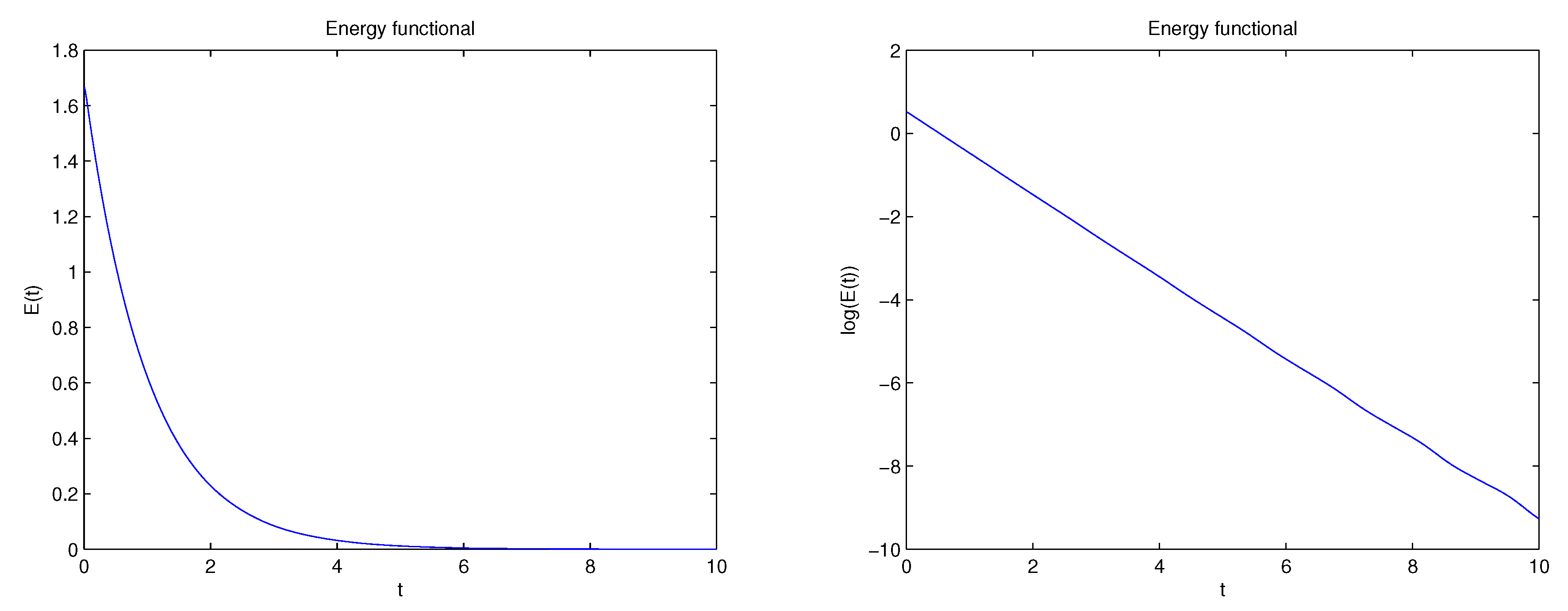
taking the discretization parameters $h=k=0.001$, the evolution in time of the discrete energy $E_n^{hk}$ defined by

$$\begin{array}{c}{\displaystyle E_n^{hk}=\frac{1}{2}\{\rho \parallel v_n^{hk}{\parallel }_Y^2+(\lambda +2\mu )\parallel {\left(u_n^{hk}\right)}_x{\parallel }_Y^2+J\parallel e_n^{hk}{\parallel }_Y^2+\gamma {({\phi }_n^{hk},{\left(u_n^{hk}\right)}_x)}_Y+a_0\parallel {\left({\phi }_n^{hk}\right)}_x{\parallel }_Y^2+\xi {\parallel {\phi }_n^{hk}\parallel }_Y^2}\hfill \\ +m{({\left({\psi }_n^{hk}\right)}_x,{\left({\phi }_n^{hk}\right)}_x)}_Y+a\parallel {\theta }_n^{hk}{\parallel }_Y^2+\kappa {\parallel {\left({\psi }_n^{hk}\right)}_x\parallel }_Y^2\},\hfill \end{array}$$

is shown in Figure 2 using both natural and semi-log scales. We can see that the discrete energy converges to zero and an exponential decay seems to be achieved.

4.3. First Two-Dimensional Example: Application of a Surface Force

As a first two-dimensional example, we consider the square domain $[0,1]\times [0,1]$, which is assumed to be clamped on its left part $\left\{0\right\}\times [0,1]$. We also suppose that the thermal displacement and porosity vanish on the whole boundary, and we use the following expression for the mechanical surface force:

$${\mathit{f}}_F(x,y,t)=(-t{y}^2,0)\mathrm{for}x=1,y\in (0,1),$$

which is assumed to be applied on the boundary ${\mathsf{\Gamma }}_F=\left\{1\right\}\times (0,1)$, a part of the whole boundary $\partial \mathsf{\Omega }$. Even if this case was not studied in the previous sections, it is straightforward to extend the analysis to this more general case.

The following data have been employed in this simulation:

$$\begin{array}{c}T=1,\rho =1,\beta =1,J=1,a=1,{\kappa }^{\ast }=1,d=1,\mu =2,\lambda =1,\hfill \\ {\mu }^{\ast }=2,{\lambda }^{\ast }=1,\gamma =2,\xi =3,m=1,a_0=2,\kappa =1,\hfill \end{array}$$

and null initial conditions for all the variables.

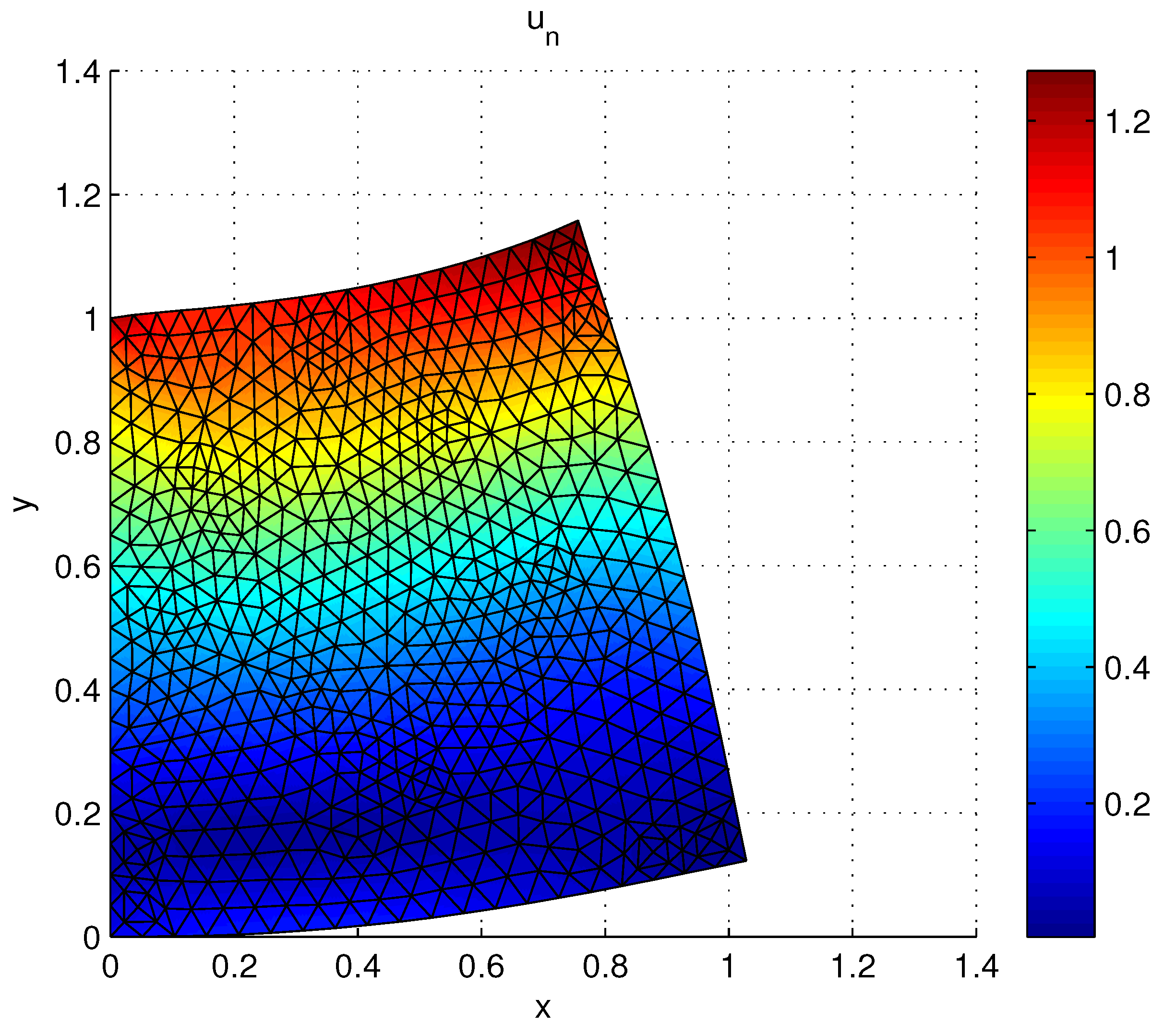
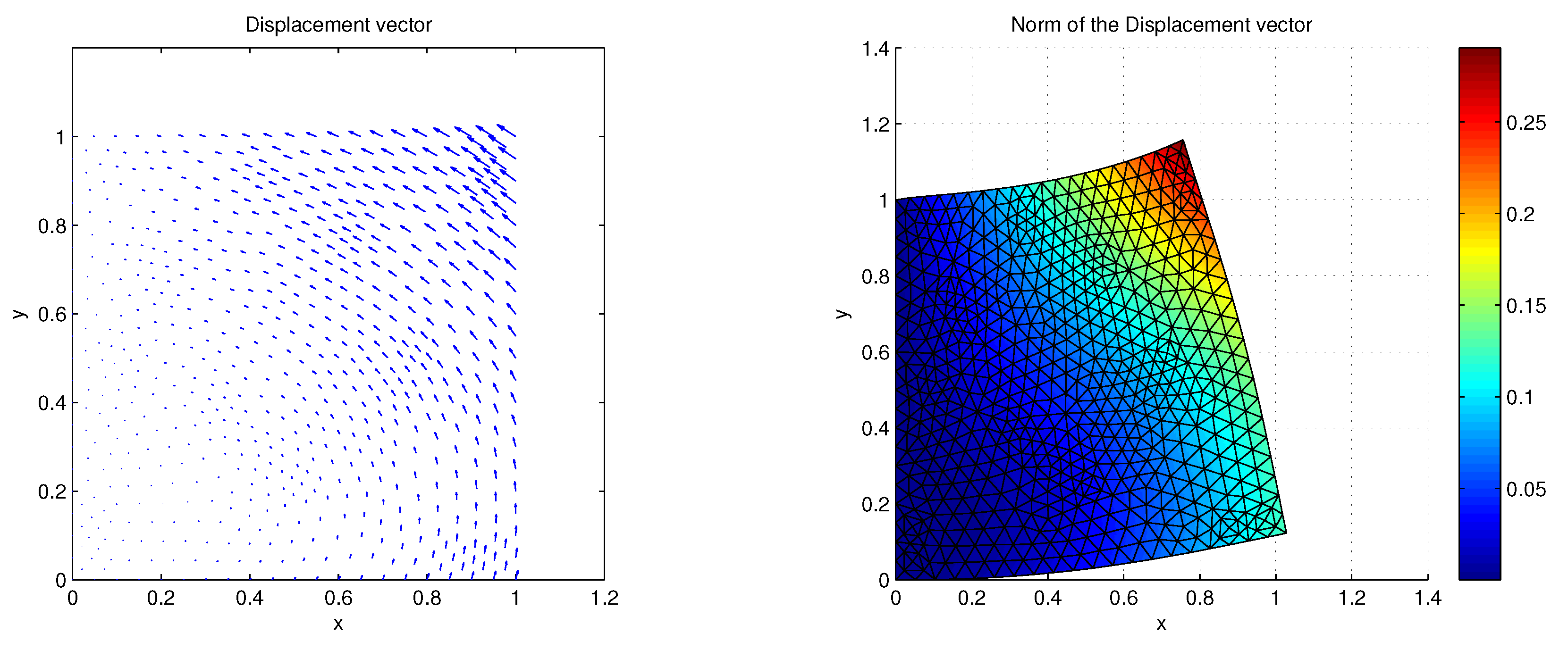
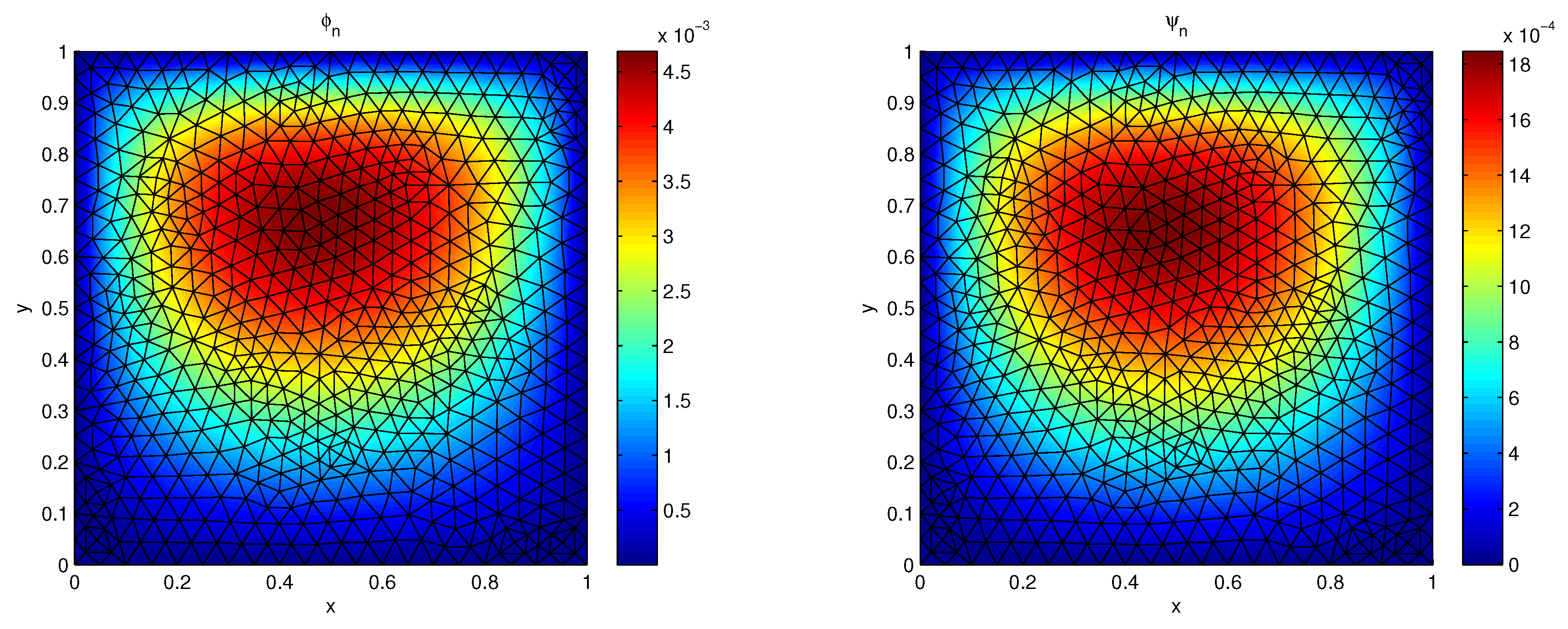
Taking the time discretization parameter $k=0.01$, the deformation generated by this mechanical force is shown in Figure 3. In Figure 4 we plot the displacement in vector arrows (on the left-hand side) and its norm (on the right-hand side) at final time. As can be seen, there is a deformation along the horizontal axis. Moreover, the porosity (left) and the thermal displacement (right) are plotted in Figure 5 at final time. We note that both neglect on the boundary due to the null boundary conditions and they are generated by the deformation of the body.

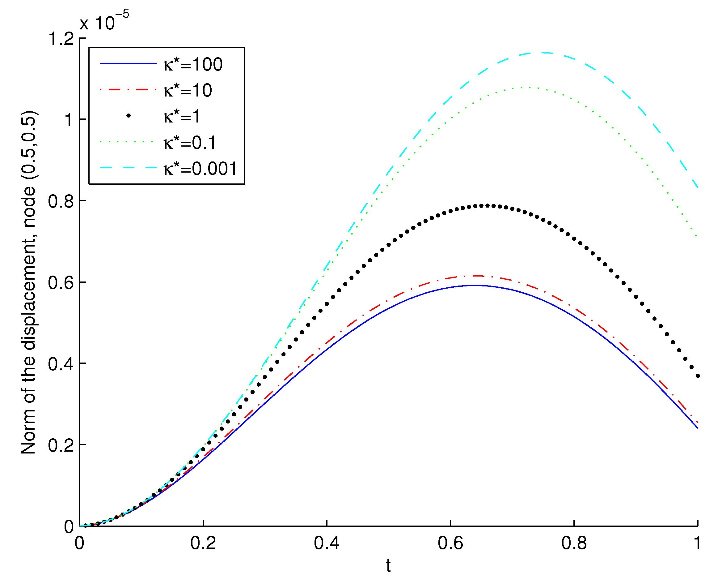
4.4. Second Two-Dimensional Example: Dependence on the Type III Thermal Coefficient

In this second two-dimensional example, we will investigate the dependence on the type III thermal coefficient ${\kappa }^{\ast }$.

In this simulation, we have used the following data:

$$\begin{array}{c}T=1,\rho =100,\beta =1,J=4,a=3,d=1,\mu =2,\lambda =1,{\mu }^{\ast }=2,\hfill \\ {\lambda }^{\ast }=1,\gamma =2,\xi =3,m=1,a_0=2,\kappa =1,\hfill \end{array}$$

with parameter ${\kappa }^{\ast }$ varying between $0.001$ and 100. No mechanical forces are now applied, and we also impose an initial condition ${\phi }_0(x,t)=e_0(x,y)=x(x-1)\ast y(y-1)$ for $(x,y)\in (0,1)\times (0,1)$, being the remaining initial conditions assumed to be zero.

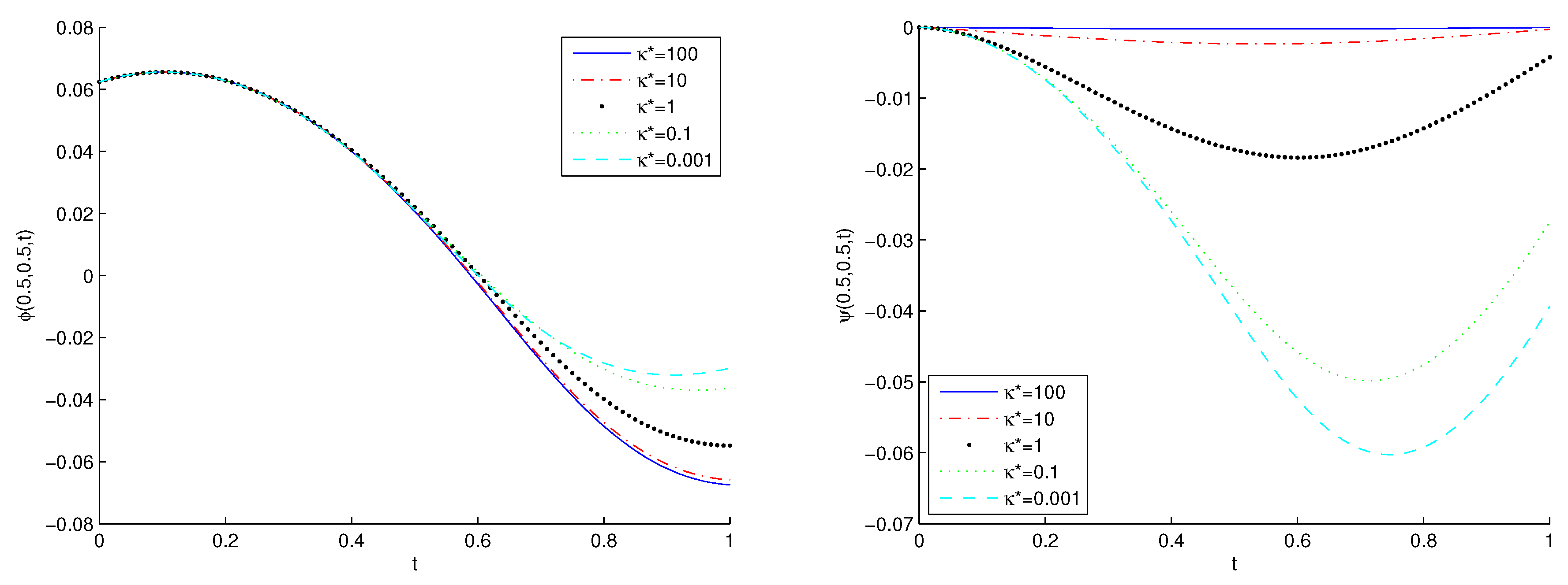
Taking the time discretization parameter $k=0.01$, the evolution in time of the norm of the displacement at middle point $\mathit{x}=(0.5,0.5)$ is shown in Figure 6. It seems that an increasing quadratic behavior is found. Moreover, in Figure 7 we plot the evolution in time of the porosity (left) and the thermal displacement (right). The porosity has an oscillating behavior and, as expected, the thermal displacement has a quadratic form, converging both variables to zero.

5. Conclusions

In this paper, we numerically analyzed a dynamic poro-thermo-viscoelastic problem within the type III thermoelasticity. The weak form led to a linear system composed of parabolic variational equations written in terms of the velocity, the volume fraction speed and the temperature. Then, using the finite element method to approximate the spatial variable and the implicit Euler scheme to discretize the time derivatives, we introduced a fully discrete scheme. A priori error estimates were proved by using a discrete version of Gronwall’s inequality. Finally, we presented a one-dimensional numerical simulation to show the convergence of the algorithm and the exponential decay of the discrete energy (Example 1), the effect of the application of a surface force (Example 2) and the dependence on the type III thermal coefficient (Example 3).

References

- Cowin, S.C.; Nunziato, J.W. Linear elastic materials with voids. J. Elast. 1983, 13, 125–147. [Google Scholar] [CrossRef]
- Nunziato, J.W.; Cowin, S. A nonlinear theory of elastic materials with voids. Arch. Ration. Mech. Anal. 1979, 415, 175–201. [Google Scholar] [CrossRef]
- Aouadi, M. Uniqueness and existence theorems in thermoelasticity with voids without energy dissipation. J. Frankl. Inst. 2012, 349, 128–139. [Google Scholar]
- Aouadi, M.; Ciarletta, M.; Iovane, G. A porous thermoelastic diffusion theory of types II and III. Acta Mech. 2017, 228, 931–949. [Google Scholar] [CrossRef]
- Apalara, T.A. Exponential decay in one-dimensional porous dissipation elasticity. Quart. J. Mech. Appl. Math. 2017, 70, 360–372. [Google Scholar] [CrossRef]
- Bazarra, N.; Fernández, J.R. Numerical analysis of a contact problem in poro-thermoelasticity with microtemperatures. Z. Angew. Math. Mech. 2018, 98, 1190–2009. [Google Scholar] [CrossRef]
- Birsan, M.; Altenbach, H. The Korn-type inequality in a Cosserat model for thin thermoelastic porous rods. Meccanica 2012, 47, 789–794. [Google Scholar] [CrossRef]
- Casas, P.S.; Quintanilla, R. Exponential decay in one-dimensional porous-thermoelasticity. Mech. Res. Comm. 2012, 40, 652–658. [Google Scholar]
- Chirita, S.; Ciarletta, M.; Straughan, B. Structural stability in porous elasticity. Proc. R. Soc. Lond. Ser. A Math. Phys. Eng. Sci. 2006, 462, 2593–2605. [Google Scholar] [CrossRef]
- Ciarletta, M.; Svanadze, M.; Buonnano, L. Plane waves and vibrations in the theory of micropolar thermoelasticity for materials with voids. Eur. J. Mech. A Solids 2009, 28, 897–903. [Google Scholar] [CrossRef]
- Fernández, J.R.; Masid, M. A porous thermoelastic problem: An a priori error analysis and computational experiments. Appl. Math. Comput. 2017, 305, 117–135. [Google Scholar] [CrossRef]
- Iesan, D. On the nonlinear theory of thermoviscoelastic materials with voids. J. Elast. 2017, 128, 1–16. [Google Scholar] [CrossRef]
- Klinkel, S.; Reichel, R. A finite element formulation in boundary representation for the analysis of nonlinear problems in solid mechanics. Comput. Methods Appl. Mech. Eng. 2019, 347, 295–315. [Google Scholar] [CrossRef]
- Magaña, A.; Quintanilla, R. On the time decay of solutions in one-dimensional theories of porous materials. Int. J. Solids Struct. 2006, 43, 3414–3427. [Google Scholar] [CrossRef] [Green Version]
- Marin, M. Some basic theorems in elastostatics of micropolar materials with voids. J. Comput. Appl. Math. 1996, 70, 115–126. [Google Scholar] [CrossRef] [Green Version]
- Marin, M. Weak solutions in elasticity of dipolar porous materials. Math. Probl. Eng. 2008, 2008, 158908. [Google Scholar] [CrossRef]
- Marin, M. An approach of a heat-flux dependent theory for micropolar porous media. Meccanica 2016, 51, 1127–1133. [Google Scholar] [CrossRef]
- Marin, M.; Chirila, A.; Öchsner, A.; Vlase, S. About finite energy solutions in thermoelasticity of micropolar bodies with voids. Bound. Value Probl. 2019, 2019, 89. [Google Scholar] [CrossRef]
- Pamplona, P.X.; Muñoz Rivera, J.E.; Quintanilla, R. On the decay of solutions for porous-elastic systems with history. J. Math. Anal. Appl. 2011, 379, 682–705. [Google Scholar] [CrossRef]
- Pamplona, P.X.; Muñoz Rivera, J.E.; Quintanilla, R. Analyticity in porous-thermoelasticity with microtemperatures. J. Math. Anal. Appl. 2012, 394, 645–655. [Google Scholar] [CrossRef]
- Iesan, D. Thermoelastic Models of Continua; Kluwer: Alphen aan den Rijn, The Netherlands, 2004. [Google Scholar]
- Straughan, B. Mathematical Aspects of Multi-Porosity Continua; Springer: Berlin, Germany, 2017. [Google Scholar]
- Green, A.E.; Naghdi, P.M. A unified procedure for contruction of theories of deformable media. I Classical continuum physics, II Generalized continua, III Mixtures of interacting continua. Proc. R. Soc. A 1995, 448, 335–356, 357–377, 379–388. [Google Scholar] [CrossRef]
- Fareh, A.; Messaoudi, S.A. Stabilization of a type III thermoelastic Timoshenko system in the presence of a time-distributed delay. Math. Nachr. 2017, 290, 1017–1032. [Google Scholar] [CrossRef]
- Jorge, M.; Pinheiro, S.B. Improvement on the polynomial stability for a Timoshenko system with type III thermoelasticity. Appl. Math. Lett. 2019, 96, 95–100. [Google Scholar] [CrossRef]
- Magaña, A.; Quintanilla, R. Exponential stability in type III thermoelasticity with microtemperatures. Z. Angew. Math. Phys. 2018, 69, 129. [Google Scholar] [CrossRef]
- Miranville, A.; Quintanilla, R. Exponential decay in one-dimensional type III thermoelasticity with voids. Appl. Math. Lett. 2019, 94, 30–37. [Google Scholar] [CrossRef]
- Mustafa, M.I. A uniform stability result for thermoelasticity of type III with boundary distributed delay. J. Math. Anal. Appl. 2014, 415, 148–158. [Google Scholar] [CrossRef]
- Prasad, R.; Das, S.; Mukhopadhyay, S. A two-dimensional problem of a mode I crack in a type III thermoelastic medium. Math. Mech. Solids 2013, 18, 506–523. [Google Scholar] [CrossRef]
- Bazarra, N.; Fernández, J.R.; Quintanilla, R. Analysis of a thermoelastic problem of type III. 2019; 277–285, unpublished work. [Google Scholar]
- Iesan, D.; Quintanilla, R. On thermoelastic bodies with inner structure and microtemperatures. J. Math. Anal. Appl. 2009, 354, 12–23. [Google Scholar] [CrossRef]
- Bazarra, N.; Fernández, J.R.; Leseduarte, M.C.; Magaña, A.; Quintanilla, R. On the uniqueness and analyticity in viscoelasticity with double porosity. Asymptot. Anal. 2019, 112, 151–164. [Google Scholar] [CrossRef] [Green Version]
- Clement, P. Approximation by finite element functions using local regularization. RAIRO Math. Model. Numer. Anal. 1975, 9, 77–84. [Google Scholar] [CrossRef]
- Andrews, K.T.; Fernández, J.R.; Shillor, M. Numerical analysis of dynamic thermoviscoelastic contact with damage of a rod. IMA J. Appl. Math. 2005, 70, 768–795. [Google Scholar]
- Campo, M.; Fernández, J.R.; Kuttler, K.L.; Shillor, M.; Viaño, J.M. Numerical analysis and simulations of a dynamic frictionless contact problem with damage. Comput. Methods Appl. Mech. Eng. 2006, 196, 476–488. [Google Scholar] [CrossRef]
Figure 1.
Example 1: Asymptotic behavior of the numerical scheme.
Figure 2.
Example 1: Discrete energy evolution in natural and semi-log scales.
Figure 3.
Example 2: Deformation and von Mises stress norm at final time.
Figure 4.
Example 2: Representation of the displacement with arrows (left) and its norm (right) at final time.
Figure 5.
Example 2: Porosity (left) and thermal displacement (right) at final time.
Figure 6.
Example3 2: Evolution in time of the norm of the displacement at point .
Figure 7.
Example 3: Evolution in time of the porosity (left) and thermal displacement (right) at point .