Propagation and Parametric Amplification in Four-Wave Mixing Processes: Intramolecular Coupling and High-Order Effects

Abstract

A strong pump-power dependence of the four-wave mixing (FWM) signal for an aqueous solution of Malachite green is reported. The characteristics of the pump-power dependence of the nonlinear signal are reproduced by a theoretical model based on the coupling between pump-probe, considering signal fields and propagation effects. The effect of the intramolecular coupling on the nonlinear intensity of the FWM signal is studied using a model molecule consisting of two-coupled harmonic curves of electronic energies with minima displaced in energy and nuclear positions. Two-vibrational states are considered while including non-adiabatic effects for the two-state model. Moreover, the coupling among the field components, as well as the propagation effects, are studied by considering a constant pump-intensity. Our calculation scheme, considering both the intramolecular coupling effects in the description of the molecular structure and the effects produced by the propagation of the FWM signal along the optical length, allows the exponential dependence of the latter, as the intensity of the pumping beam increases. Our treatments do not require the inclusion of other non-resonant processes outside the RWA approximation, due to the consideration of an adiabatic basis.

1. Introduction

Multiphoton processes of intense electromagnetic fields interacting with molecular systems are phenomena of interest with a great variety of applications [1,2,3,4,5,6] in non-linear optics. With respect to these, Fong and Shen refer to cases characterized by a strong coupling between light and matter, where the usual prescription derived from perturbation methods are no longer valid [7]. In 1989, Burnett and Hutchinson dedicated a special issue to multiphoton interactions in intense laser fields [8]. In 2013, Zhang et al. [9] studied the deviation of the absorption feature in the resonance-enhanced multiphoton ionization (REMPI) process as a function of resonance detuning. One of the most interesting spectroscopic techniques corresponds to four-wave mixing, both in the degenerate and nondegenerate cases, given its multiple applications in the characterization of molecular systems, particularly in polymers [10], biological molecules [11], nanometric semiconductor clusters [12], and excitons [13]. More recently, Al-Saidi and Abdulkareen [14] reported changes in the optical responses of chemical solutions in terms of the concentration of the analyzed organic dye, where the system response to the variation of the concentration is produced by the induced high nonlinear saturable absorption, an issue of importance for the development of optical limiters. The effect of propagation on pulsed four-wave mixing [15], counter-propagating spontaneous four-wave mixing [16], and the theory of propagation effects in time-resolved four-wave mixing [17], highlights the relevance of knowing how these beams behave once they penetrate an optical length, where absorption and scattering processes play an important role for the understanding of propagation, as well as being able to correctly decipher some symmetry properties inherent to both incident and emergent fields. Studies using FWM techniques have derived general formalisms, which include the Stark effect applied to the understanding of the instabilities occurring in electromagnetic fields through absorption media [18]. Many phenomena associated with radiation-matter interaction are observed when electromagnetic fields pass through an optical path [19]. Some authors have focused on developments of methodologies based on Wei–Norman algebra applied to field propagation through homogeneous systems, with analogies between the evolution operator and optical propagation matrices. Other studies on the effect of electromagnetic field propagation in a homogeneous spectral distribution of the FWM signal have employed models where the intensity of the pumping beam is constant along its optical path [20,21]. Normally, the study of the optical propagation of FWM signals is based on modeling, considering the molecule as a two-level system; therefore, disregarding the molecular structure that embodies the active subsystem that interacts with the radiation.

In the present study, we present the propagation of the dynamic fields associated with the FWM signal, where it is necessary to consider the implicit effects of absorption and scattering along the optical length. The theoretical development of nonlinear optical properties allows us to establish the relationship between the characteristics of the material (e.g., molecular structure, chemical composition, etc.) and the nature of the radiative perturbation [22,23]. The nonlinear absorption coefficient and refractive index depend on the system susceptibility, which depends on the electric dipole moment [24]. This plays an essential role in dye production processes and the design of new materials. Despite its importance, several authors [25,26,27] have estimated values of nonlinear optical responses based on constant electric dipole moments; however, the electric dipole moments are strongly influenced by phenomena such as intramolecular coupling [28,29,30,31,32,33], which defines the interaction between nuclear motion and electronic motion in a polyatomic system, and which produces a displacement of the energy levels of the electronic states of the material, affecting its electronic distribution [34,35,36].

Vibronic coupling is required to correct a system’s Born–Oppenheimer wave functions by altering the electric dipole moment. Analysis of intramolecular coupling provides relevant information about the phenomena which relate to the appearance of “symmetry-forbidden” electronic transitions in absorption spectra [29] or the molecular instability of systems with configurations in electronically degenerate states through the Jahn–Teller effect [34]. At the same time, insights concerning the interpretation of tunnelling microscopy images of Fullerene anions [33], tunnelling spectroscopy of inelastic electrons [37], the relationship with the chemical potential and how it enhances intermolecular charge transfer [38], as well as the design of high spin molecules [39], can be obtained by the application of these models. Our analysis in the present paper aims to examine the propagation of the nondegenerate four-wave mixing signal along a defined optical length, which is subject to the saturative effects of the intense pump field and the details of the molecular structure in terms of vibronic coupling. In this analysis, we note from the results obtained the correlation between the optical responses and the molecular structure, as well as the exponential dependence of the FWM signal intensity on the pump intensity, in terms of a parametric amplification tunable to the organic dye. Similar treatments in a two-level system, without considering the details of vibronic coupling, where higher order effects of the pumping beam on this same organic Malachite green dye are studied using Rayleigh-type optical mixing RTOM techniques in an absorbing medium, show that it is more sensitive to saturation than to the effects that can be expected from saturation-absorption arguments [40].

The article is organized as follows: Section 2 dedicated to the model. Section 2.1 considers the molecular model and is dedicated to constructing the permanent and transition dipole moments in the adiabatic representation, i.e., using both the new wave functions generated from the crossing of harmonic states. The product of the variational resolution of the problem provides the new energies of the system and, with it, the Bohr frequency of the new adiabatic states. In Section 2.2, relating to the radiation-matter interaction model, we solve the optical Bloch equations (OBE) in the frequency domain for the electromagnetic fields considered in the FWM signal and, with them, the corresponding induced nonlinear macroscopic polarization and propagation effects are discussed in Section 2.3. Here, we consider the resolution of the amplitude variations of the incident and generated beams in the optical path as they pass through a defined optical length. Section 3 is dedicated to the results and discussion, and, in Section 4, the final comments and conclusions are provided.

2. Models

The study object of this work corresponds to the analysis of the behavior of the four-wave mixing signal in the optical transit, considering intensities and angular arrangements of the incident fields, molecular structure effects, optical path length, among others. This involves modeling how to represent the system of states in diabatic and adiabatic configurations, interaction of radiation with matter in dipole-electric approximations, system responses in terms of susceptibility, induced polarizations, and changes in the intensities of the various fields, according to the optical path.

2.1. Molecular Model of a Two-Level System with Intramolecular Coupling

The intramolecular coupling is associated with the crossing of two or more potential energy curves that results from the interplay between the electronic and nuclear motions in molecules. The resulting effects have been envisaged as linear or quadratic terms describing the dynamics of the nuclei. To solve the problems involving more than one potential surface, one can resort to the Born–Oppenheimer separation of the Schrödinger equation, which results in a set of differentials coupled equations describing the nuclei dynamics within the adiabatic approximation. 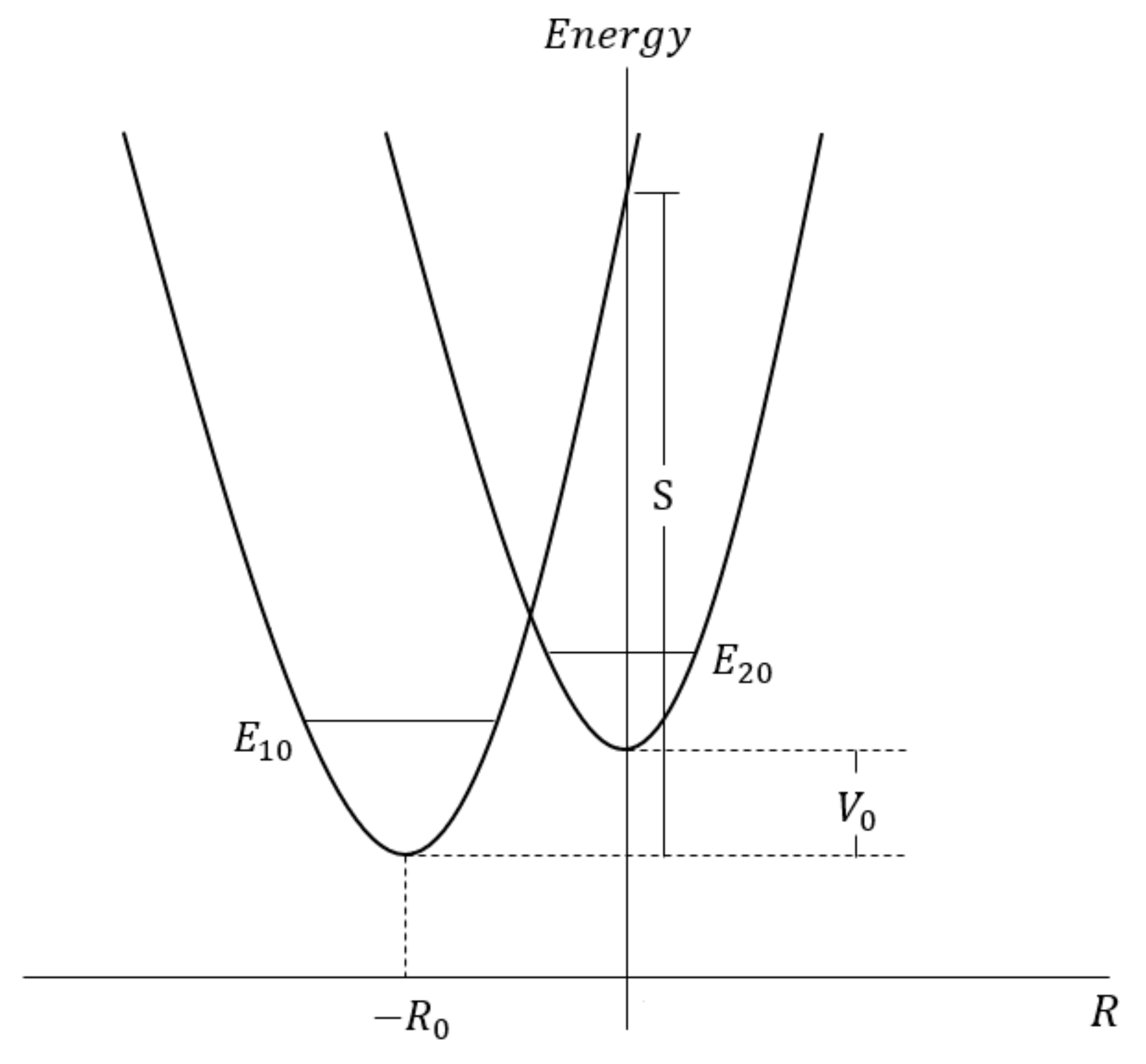Moreover, the effect of intramolecular coupling on the system response can be represented by considering two electronic states ${\mathsf{\phi }}_1(\mathrm{r};\mathrm{R})$ and ${\mathsf{\phi }}_2(\mathrm{r};\mathrm{R})$, where r and R, are the collective electronic coordinates and the nuclear position, respectively. This model can be employed for describing diatomic molecules and can also be extended to an optically active model of polyatomic molecules. As depicted in Figure 1, the electronic states are represented by two one-dimensional crossed harmonic potential curves which have a minimal horizontal displacement along the nuclear coordinate, ${\mathrm{R}}_0$, and a vertical displacement in energy ${\mathrm{V}}_0$. Finally, each electronic state is characterized by its own fundamental vibrational state, represented by the wave functions ${\mathsf{\varphi }}_{10}(\mathrm{R})$ and ${\mathsf{\varphi }}_{20}(\mathrm{R})$, with energy values ${\mathrm{E}}_{10}$ and ${\mathrm{E}}_{20}$.

It is of paramount importance to recognize that the validity of a model that considers only two vibrational states depends on the separation of the energy existing between the minima of the electronic curves. The latter implies that the coupling parameters between the two states are small in comparison to the vibrational energy of both oscillators. In the same context, the two potential curves are considered to possess different frequency constants ${\mathsf{\omega }}_0^{\mathrm{HO}}$ and ${\tilde{\mathsf{\omega }}}_0^{\mathrm{HO}}$, which are related as $\mathsf{\delta }={\tilde{\mathsf{\omega }}}_0^{\mathrm{HO}}/{\mathsf{\omega }}_0^{\mathrm{HO}}$. From the above electronic states, a trial wave function is defined as follows:

$$\mathrm{\Psi }(\mathrm{r},\mathrm{R})={\mathrm{C}}_{10}{\mathsf{\varphi }}_{10}(\mathrm{R}){\mathsf{\phi }}_1(\mathrm{r};\mathrm{R})+{\mathrm{C}}_{20}{\mathsf{\varphi }}_{20}(\mathrm{R}){\mathsf{\phi }}_2(\mathrm{r};\mathrm{R})$$

(1)

where the coefficients ${\mathrm{C}}_{10}$ and ${\mathrm{C}}_{20}$ are to be obtained by means variationally. The molecular Hamiltonian is: $\mathrm{H}(\mathrm{r},\mathrm{R})=\mathrm{T}+\mathrm{V}(\mathrm{r},\mathrm{R})+\tilde{\mathrm{H}}(\mathrm{r})$, where $\mathrm{T}$ is the kinetic energy operator, $\mathrm{V}(\mathrm{r},\mathrm{R})$ is the potential energy operator arising from the electrostatic interactions between electrons and nuclei, and $\tilde{\mathrm{H}}(\mathrm{r})$ is a residual electronic interaction, which is coupled to the two considered vibronic states represented by the Born–Oppenheimer product of its electronic function ${\mathsf{\phi }}_{\mathrm{m}}(\mathrm{r};\mathrm{R})$ and its vibrational function ${\mathsf{\varphi }}_{\mathrm{m}\mathrm{n}}(\mathrm{R})$ with m = 1,2. Finally, “$\mathsf{\nu }$” in Figure 1 is the intramolecular coupling parameter and “S” is the energy at which the crossing occurs. The residual perturbation $\tilde{\mathrm{H}}(\mathrm{r})$ can be readily computed as the following integral:

$$\left.〈{\mathsf{\varphi }}_{10}{\mathsf{\phi }}_1\right|\tilde{\mathrm{H}}(\mathrm{r})\left|{\mathsf{\varphi }}_{20}{\mathsf{\phi }}_2\right.〉=\mathsf{\nu }\left.〈{\mathsf{\varphi }}_{10}\right|{\mathsf{\varphi }}_{20}〉={\mathsf{\Gamma }}_{00}$$

(2)

where $\mathsf{\nu }$ is defined as: $\left.〈{\mathsf{\phi }}_1\right|\tilde{\mathrm{H}}(\mathrm{r})\left|{\mathsf{\phi }}_2\right.〉=\mathsf{\nu }$. The diagonal elements of the secular determinant associated to (2) are the energy of the harmonic oscillator with angular frequency ${\mathsf{\omega }}_0^{\mathrm{H}\mathrm{O}}$ and displacement in energy ${\mathrm{V}}_0$. In this context, $\mathsf{\nu }$ is the coupling between the diabatic electronic states, and the overlap $\left.〈{\mathsf{\varphi }}_{10}\right|{\mathsf{\varphi }}_{20}〉$ between the vibrational functions. The latter overlap can be obtained by means of Pekarian’s formula [35], where different force constants can be introduced. Pekarian’s formula is defined as follows:

$$\left.〈{\mathsf{\varphi }}_{10}\right|{\mathsf{\varphi }}_{20}〉=\frac{{\left(4\mathsf{\delta }\right)}^{1/4}}{{\left(1+\mathsf{\delta }\right)}^{1/2}}\exp \left[-\frac{\mathrm{S}}{2}\left(1-{\left(1+\mathsf{\delta }\right)}^{-1}\right)\right]$$

(3)

where $\mathrm{S}=\left(\mathrm{m}{\mathsf{\omega }}_0/ħ\right){\mathrm{R}}_0^2$ corresponds to the energy height at which the coupling occurs, m is the reduced mass associated with the vibrational mode ${\mathrm{R}}_0$ and frequency ${\mathsf{\omega }}_0$. By solving (1), the coupled eigenstates of the system are obtained as:

$${\mathrm{\Psi }}_{\mathrm{P}}(\mathrm{r},\mathrm{R})=\frac{{\left|{\mathsf{\Gamma }}_{00}\right|}^2}{\sqrt{{\left|{\mathsf{\Gamma }}_{00}\right|}^2+{\left({\mathrm{E}}_{10}-{\mathrm{E}}_{\mathrm{J}}\right)}^2}}\left\{{\mathsf{\phi }}_1(\mathrm{r};\mathrm{R}){\mathsf{\varphi }}_{1\mathrm{j}}(\mathrm{R})\pm \frac{\left({\mathrm{E}}_{10}-{\mathrm{E}}_{\mathrm{P}}\right)}{{\mathsf{\Gamma }}_{00}}{\mathsf{\phi }}_2(\mathrm{r};\mathrm{R}){\mathsf{\varphi }}_{2\mathrm{k}}(\mathrm{R})\right\}$$

(4)

where the energies are given by:

$${\mathrm{E}}_{\mathrm{P}}=\frac{1}{2}\left({\mathrm{E}}_{10}+{\mathrm{E}}_{20}\right)\pm \frac{1}{2}{\left[{\left({\mathrm{E}}_{10}-{\mathrm{E}}_{20}\right)}^2+4{\left|{\mathsf{\Gamma }}_{00}\right|}^2\right]}^{1/2}$$

(5)

with ${\mathrm{E}}_{10}=0.5$ and ${\mathrm{E}}_{20}=0.5\mathsf{\delta }+{\mathrm{V}}_0$. Furthermore, $\mathrm{p}=\mathrm{A}$ for (−) sign and B for (+) sign.

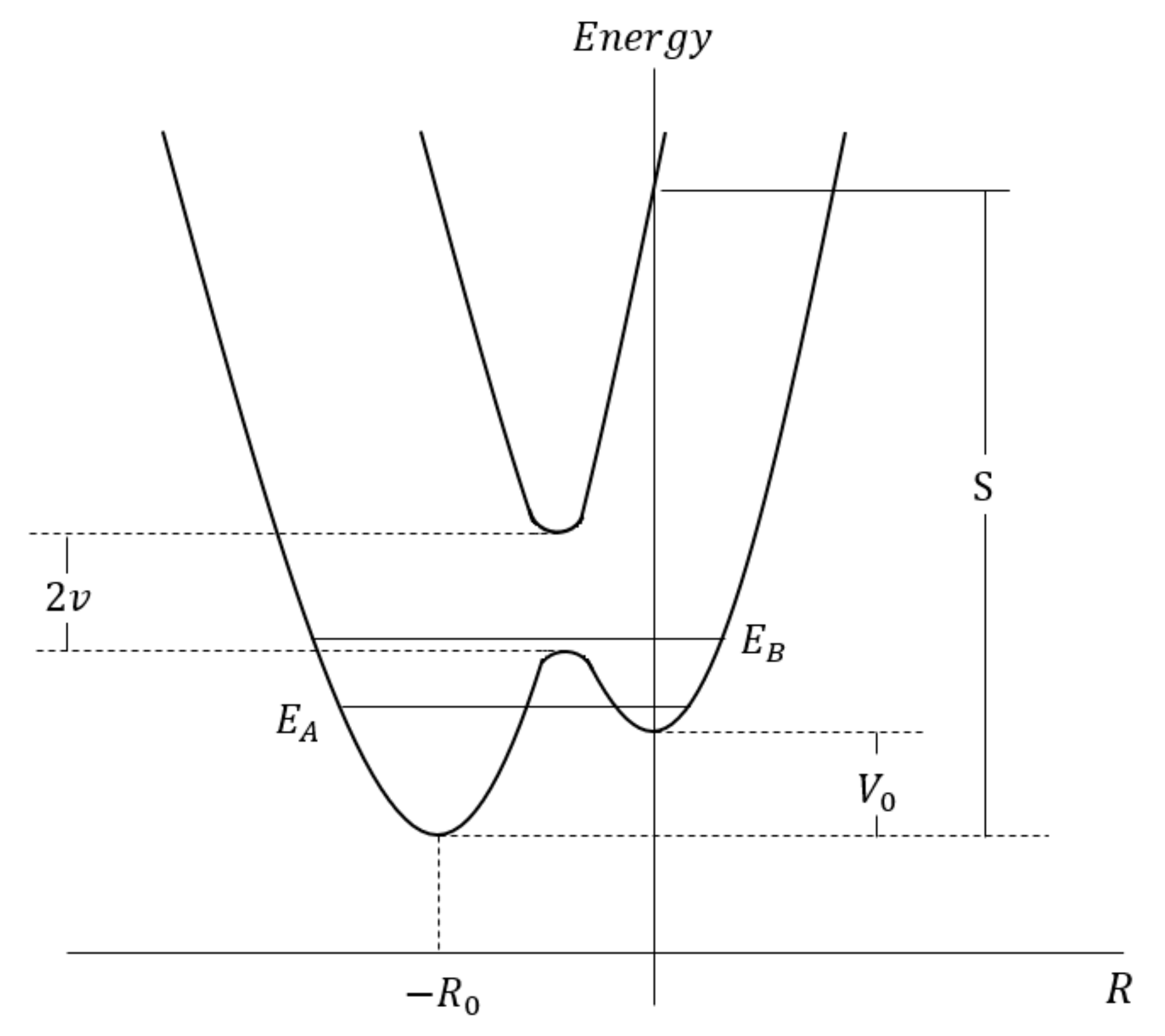
Upon the inclusion of $\tilde{\mathrm{H}}(\mathrm{r})$ in the Hamiltonian system, the two-potential energy curves, as well as the wavefunctions of Figure 1, result in separation as a result of the changes in ${\mathrm{E}}_{10}$ and ${\mathrm{E}}_{20}$ (Figure 2), where

$$\mathrm{H}(\mathrm{r},\mathrm{R})\left|{\mathrm{\Psi }}_{\mathrm{A}}\right.〉={\mathrm{E}}_{\mathrm{A}}\left|{\mathrm{\Psi }}_{\mathrm{A}}\right.〉$$

(6)

$$\mathrm{H}(\mathrm{r},\mathrm{R})\left|{\mathrm{\Psi }}_{\mathrm{B}}\right.〉={\mathrm{E}}_{\mathrm{B}}\left|{\mathrm{\Psi }}_{\mathrm{B}}\right.〉$$

(7)

Here, the fundamental and excited state wavefunctions ${\mathrm{E}}_{\mathrm{A}}$ and ${\mathrm{E}}_{\mathrm{B}}$ are defined by their respective energies. The wavefunctions $\left|{\mathrm{\Psi }}_{\mathrm{A}}\right.〉$ and $\left|{\mathrm{\Psi }}_{\mathrm{B}}\right.〉$ in the Born–Oppenheimer approximation are defined as: $\left|{\mathrm{\Psi }}_{\mathrm{A}}\right.〉=\left|{\mathsf{\varphi }}_{1\mathrm{j}}{\mathsf{\phi }}_1\right.〉$ and $\left|{\mathrm{\Psi }}_{\mathrm{B}}\right.〉=\left|{\mathsf{\varphi }}_{2\mathrm{k}}{\mathsf{\phi }}_2\right.〉$. The eigenvectors corresponding to the eigenvalues ${\mathrm{E}}_{\mathrm{A}}$ and ${\mathrm{E}}_{\mathrm{B}}$ are:

$$\left|{\mathrm{\Psi }}_{\mathrm{B}}\right.〉={\mathrm{C}}_{\mathrm{j}\mathrm{k}}^{\mathrm{B}}\left({\mathsf{\varphi }}_{1\mathrm{j}}{\mathsf{\phi }}_1-{\mathrm{D}}_{\mathrm{j}\mathrm{k}}^{\mathrm{B}}{\mathsf{\varphi }}_{2\mathrm{k}}{\mathsf{\phi }}_2\right) \mathrm{and} \left|{\mathrm{\Psi }}_{\mathrm{A}}\right.〉={\mathrm{C}}_{\mathrm{j}\mathrm{k}}^{\mathrm{A}}\left({\mathsf{\varphi }}_{1\mathrm{j}}{\mathsf{\phi }}_1-{\mathrm{D}}_{\mathrm{j}\mathrm{k}}^{\mathrm{A}}{\mathsf{\varphi }}_{2\mathrm{k}}{\mathsf{\phi }}_2\right)$$

(8)

$${\mathrm{C}}_{\mathrm{j}\mathrm{k}}^{\mathrm{q}}=\frac{1}{\sqrt{1+{\left({\mathrm{D}}_{\mathrm{j}\mathrm{k}}^{\mathrm{q}}\right)}^2}} \mathrm{and} {\mathrm{D}}_{\mathrm{j}\mathrm{k}}^{\mathrm{q}}=\frac{\left({\mathrm{E}}_{1\mathrm{j}}-{\mathrm{E}}_{\mathrm{q}}\right)}{{\mathsf{\Gamma }}_{00}}, \mathrm{q}=\mathrm{A},\mathrm{B}.$$

(9)

Because of its construction, our model considers a marked influence of the magnitudes of both the permanent and transition dipole moments in the FWM signal response. The following integral gives these expressions:

$${\mathrm{m}}_{\mathrm{p},\mathrm{k}}(\mathrm{R})={\displaystyle \underset{-\infty }{\overset{\infty }{\int }}{\mathsf{\phi }}_{\mathrm{p}}^{*}(\mathrm{r};\mathrm{R})\stackrel{⌢}{\mathrm{m}}{\mathsf{\phi }}_{\mathrm{k}}(\mathrm{r};\mathrm{R}){\mathrm{d}}^3\mathrm{r}}$$

(10)

where $\widehat{\mathrm{m}}$ is the operator associated with the total electronic dipole moment. A new set of dipole moments can be obtained based on the coupled states, being different to the set belonging to the solution of the uncoupled case. Moreover, it has been shown elsewhere [28,29,31] that null dipole moments in the uncoupled basis do not necessarily imply the nullity of the dipole moments in the new generated basis. The expressions describing these quantities are written as follows:

$${\mathsf{\mu }}_{\mathrm{A}\mathrm{A}}=\left\{\frac{1}{2{\left|{\mathsf{\Gamma }}_{00}\right|}^2+\left({\mathrm{E}}_{10}-{\mathrm{E}}_{\mathrm{A}}\right){\mathsf{\epsilon }}_{12}}\right\}\left\{\left[\left({\mathrm{E}}_{10}-{\mathrm{E}}_{\mathrm{A}}\right){\mathsf{\epsilon }}_{12}+{\left|{\mathsf{\Gamma }}_{00}\right|}^2{\mathrm{m}}_{22}-{\mathrm{m}}_{11}{\left|{\mathsf{\Gamma }}_{00}\right|}^2\right]-\frac{2\left({\mathrm{E}}_{10}-{\mathrm{E}}_{\mathrm{A}}\right){\mathrm{m}}_{12}{\left|{\mathsf{\Gamma }}_{00}\right|}^2}{\mathsf{\nu }}\right\}$$

(11)

$${\mathsf{\mu }}_{\mathrm{B}\mathrm{B}}=\left\{\frac{1}{2{\left|{\mathsf{\Gamma }}_{00}\right|}^2+\left({\mathrm{E}}_{10}-{\mathrm{E}}_{\mathrm{B}}\right){\mathsf{\epsilon }}_{12}}\right\}\left\{\left[\left({\mathrm{E}}_{10}-{\mathrm{E}}_{\mathrm{B}}\right){\mathsf{\epsilon }}_{12}+{\left|{\mathsf{\Gamma }}_{00}\right|}^2{\mathrm{m}}_{22}-{\mathrm{m}}_{11}{\left|{\mathsf{\Gamma }}_{00}\right|}^2\right]-\frac{2\left({\mathrm{E}}_{10}-{\mathrm{E}}_{\mathrm{B}}\right){\mathrm{m}}_{12}{\left|{\mathsf{\Gamma }}_{00}\right|}^2}{\mathsf{\nu }}\right\}$$

(12)

$${\mathsf{\mu }}_{\mathrm{A}\mathrm{B}}={\left(\frac{{\left|{\mathsf{\Gamma }}_{00}\right|}^2}{4{\left|{\mathsf{\Gamma }}_{00}\right|}^2+{\mathsf{\epsilon }}_{12}^2}\right)}^{1/2}\left\{\left({\mathrm{m}}_{11}-{\mathrm{m}}_{22}\right)-\frac{{\mathrm{m}}_{12}{\mathsf{\epsilon }}_{12}}{\mathsf{\nu }}\right\}$$

(13)

where the quantities ${\mathrm{m}}_{\mathrm{i}\mathrm{i}}$ and ${\mathrm{m}}_{\mathrm{i}\mathrm{j}}$ are the permanent and transition dipole moments between the uncoupled states; ${\mathsf{\epsilon }}_{12}={\mathrm{E}}_{10}-{\mathrm{E}}_{20}$. It is important to note that ${\mathsf{\mu }}_{\mathrm{a}\mathrm{a}}$ and ${\mathsf{\mu }}_{\mathrm{A}\mathrm{B}}$ are the critical quantities for our analysis since they replace the conventional dipole moments of the adiabatic representation in the formulation or radiation-matter interactions. These new dipoles can be nonzero, even though the molecule may have a permanent net dipole moment equal to zero; ${\mathrm{m}}_{12}(-{\mathrm{R}}_0)$ is the dipole moment associated with the transition between diabatic states, while ${\mathrm{m}}_{11}(-{\mathrm{R}}_0)$ and ${\mathrm{m}}_{22}(0)$ are the permanent dipole moments in the diabatic states. It is important to point out that for ${\mathrm{m}}_{11}={\mathrm{m}}_{22}=0$ in Equation (10), the coupling induces a nonzero moment in the coupled states provided by ${\mathrm{m}}_{12}\ne 0$. When the ${\mathrm{m}}_{11},{\mathrm{m}}_{22}$ values are not zero, the contributions from ${\mathrm{m}}_{11}$ and ${\mathrm{m}}_{22}$ to ${\mathsf{\mu }}_{\mathrm{a}\mathrm{a}}\left(\mathrm{a}=\mathrm{A},\hspace{0.33em}\mathrm{B}\right)$ may differ substantially due to both the coupling and the Franck–Condon factors, while the only means for the permanent dipole moments to contribute to ${\mathsf{\mu }}_{\mathrm{A}\mathrm{B}}$ is through the ${\mathrm{m}}_{11}-{\mathrm{m}}_{22}$ difference. With respect to ${\mathsf{\mu }}_{\mathrm{A}\mathrm{B}}$, it is clear that it may vanish as an effect of the intramolecular coupling regardless of when ${\mathrm{m}}_{12}\ne 0$. Indeed, by considering that $\mathsf{\nu }=-{\mathrm{m}}_{12}\left({\mathrm{E}}_{1\mathrm{j}}-{\mathrm{E}}_{2\mathrm{k}}\right)/\left({\mathrm{m}}_{22}-{\mathrm{m}}_{11}\right)$, the conditions for the mentioned effect are two-fold: (i) the two states mixed by the intramolecular coupling must be nondegenerate, and (ii) the signs of ${\mathrm{m}}_{12}\left({\mathrm{E}}_{1\mathrm{j}}-{\mathrm{E}}_{2\mathrm{k}}\right)$ and ${\mathrm{m}}_{22}-{\mathrm{m}}_{11}$ must be opposite. Finally, for the degenerated case ${\mathrm{E}}_{1\mathrm{j}}={\mathrm{E}}_{2\mathrm{k}}$, ${\mathsf{\mu }}_{\mathrm{A}\mathrm{B}}$ and ${\mathsf{\mu }}_{\mathrm{a}\mathrm{a}}\left(\mathrm{a}=\mathrm{A},\hspace{0.33em}\mathrm{B}\right)$ become

$${\mathsf{\mu }}_{\mathrm{A}\mathrm{B}}=\frac{1}{2}\left[{\mathrm{m}}_{11}(-{\mathrm{R}}_0)-{\mathrm{m}}_{22}(0)\right]$$

(14)

$${\mathsf{\mu }}_{\mathrm{A}\mathrm{A}}=\frac{1}{2}\left[{\mathrm{m}}_{11}(-{\mathrm{R}}_0)+{\mathrm{m}}_{22}(0)\right]-\left[\left.〈{\mathsf{\varphi }}_{1\mathrm{j}}\right|{\mathsf{\varphi }}_{2\mathrm{k}}〉{\mathrm{m}}_{12}(-{\mathrm{R}}_0)\right]$$

(15)

$${\mathsf{\mu }}_{\mathrm{B}\mathrm{B}}=\frac{1}{2}\left[{\mathrm{m}}_{11}(-{\mathrm{R}}_0)+{\mathrm{m}}_{22}(0)\right]+\left[\left.〈{\mathsf{\varphi }}_{1\mathrm{j}}\right|{\mathsf{\varphi }}_{2\mathrm{k}}〉{\mathrm{m}}_{12}(-{\mathrm{R}}_0)\right]$$

(16)

Equations (14)–(16) represent the transition and permanent dipole moments in the adiabatic states as a function of the dipole moments of the diabatic base initially considered. It is important to note that the nondiagonal elements of the dipole moment in the adiabatic basis only depend on the permanent dipoles in the diabatic basis, unlike the permanent dipole moments in the $\left|\mathrm{A}\right.〉$ and $\left|\mathrm{B}\right.〉$ states which show dependence on both diabatic dipole moments.

2.2. Radiation-Matter Interaction Model

The aim of the present investigation is to comprehensively study the nondegenerate FWM spectroscopy of two incident beams of light on condensed phases. The first is a relatively strong light beam (pump beam) of optical frequency ${\mathsf{\omega }}_1$ and spatial propagation direction ${\overrightarrow{\mathrm{k}}}_1$; whereas the second is a weaker light beam (probe beam) which has the propagation’s optical frequency ${\mathsf{\omega }}_2$ and spatial direction ${\overrightarrow{\mathrm{k}}}_2$. By considering the latter, the generated nonlinear signal is characterized by the frequency ${\mathsf{\omega }}_3={\mathsf{\omega }}_1+\Delta$, where the detuning frequency is $\Delta ={\mathsf{\omega }}_1-{\mathsf{\omega }}_2$ and the propagation vector is defined as ${\overrightarrow{\mathrm{k}}}_3\approx 2{\overrightarrow{\mathrm{k}}}_1-{\overrightarrow{\mathrm{k}}}_2$. To describe the temporal evolution of the system, we start with the Liouville-von Newmann equation [41]:

$$\mathrm{i}ħ{\partial }_{\mathrm{t}}\mathsf{\rho }(\mathrm{t})=\left[\mathrm{H},\mathsf{\rho }(\mathrm{t})\right]$$

(17)

where $\mathsf{\rho }(\mathrm{t})$ is the density matrix and $\mathrm{H}$ is the total Hamiltonian of the complete system. In this paper, we have defined the Hamiltonian of the following form: $\mathrm{H}={\mathrm{H}}_{\mathrm{S}}+{\mathrm{H}}_{\mathrm{S}-\mathrm{F}}+{\mathrm{H}}_{\mathrm{S}-\mathrm{T}\mathrm{R}}+{\mathrm{H}}_{\mathrm{F}-\mathrm{T}\mathrm{R}}$, where ${\mathrm{H}}_{\mathrm{S}}$ corresponds to the Hamiltonian that describes the isolated system, given in this work by ${\mathrm{H}}_{\mathrm{S}}={\mathrm{H}}_0(\mathrm{r},\mathrm{R})+\tilde{\mathrm{H}}(\mathrm{r})$, where ${\mathrm{H}}_0(\mathrm{r},\mathrm{R})$ corresponds to the unperturbed system and $\tilde{\mathrm{H}}(\mathrm{r})$ represents the residual perturbation related to the intramolecular coupling. The terms ${\mathrm{H}}_{\mathrm{S}-\mathrm{F}}$, ${\mathrm{H}}_{\mathrm{S}-\mathrm{T}\mathrm{R}}$ and ${\mathrm{H}}_{\mathrm{F}-\mathrm{T}\mathrm{R}}$ represent the interaction between a molecular system and a field (F) (dipolar approximation), an interaction between the system and a thermal reservoir, and finally, an interaction between the field and thermal reservoir, respectively. However, this last term will not be considered in this model, because the solvent will be transparent to a frequency of the incident field. In view of the above considerations, the optical conventional Bloch equations (OCBE) for the system defined in terms of the uncoupled basis (considering only the intramolecular coupling) are [42,43,44,45,46]:

$${\partial }_{\mathrm{t}}{\mathsf{\rho }}_{\mathrm{B}\mathrm{A}}+\left(\frac{1}{{\tilde{\mathrm{T}}}_2}+\mathrm{i}{\mathsf{\omega }}_0^{\mathrm{A}\mathrm{B}}\right){\mathsf{\rho }}_{\mathrm{B}\mathrm{A}}=-\frac{\mathrm{i}}{ħ}{\mathrm{H}}_{\mathrm{B}\mathrm{A}}{\mathsf{\rho }}_{\mathrm{D}}$$

(18)

$${\partial }_{\mathrm{t}}{\mathsf{\rho }}_{\mathrm{D}}+\frac{1}{{\mathrm{T}}_1}\left({\tilde{\mathsf{\rho }}}_{\mathrm{D}}-{\mathsf{\rho }}_{\mathrm{D}}^{(0)}\right)=-\frac{2\mathrm{i}}{ħ}{\mathrm{H}}_{\mathrm{A}\mathrm{B}}{\mathsf{\rho }}_{\mathrm{B}\mathrm{A}}+\frac{2\mathrm{i}}{ħ}{\mathsf{\rho }}_{\mathrm{A}\mathrm{B}}{\widehat{\mathrm{H}}}_{\mathrm{B}\mathrm{A}}$$

(19)

$${\partial }_{\mathrm{t}}{\mathsf{\rho }}_{\mathrm{A}\mathrm{B}}={\partial }_{\mathrm{t}}{\mathsf{\rho }}_{\mathrm{B}\mathrm{A}}^{*}$$

(20)

where

$${\mathrm{H}}_{\mathrm{B}\mathrm{A}}=\left(\frac{{\mathsf{\nu }}^2{\mathrm{e}}^{-\mathrm{S}/2}}{4{\mathsf{\nu }}^2{\mathrm{e}}^{-\mathrm{S}/2}+{\mathrm{V}}_0}\right)\left[\left({\mathrm{m}}_{11}-{\mathrm{m}}_{22}\right)+\frac{{\mathrm{V}}_0{\mathrm{m}}_{12}}{\mathsf{\nu }}\right]\mathrm{E}(\mathrm{t})$$

(21)

$$\frac{1}{{\tilde{\mathrm{T}}}_2}=\frac{1}{{\mathrm{T}}_2}+\frac{\mathrm{i}}{ħ}\left[\frac{{\mathrm{V}}_0\left({\mathrm{m}}_{11}-{\mathrm{m}}_{22}\right)-4\mathsf{\nu }{\mathrm{e}}^{-\mathrm{S}/2}{\mathrm{m}}_{22}}{\sqrt{4{\mathsf{\nu }}^2{\mathrm{e}}^{-\mathrm{S}/2}+{\mathrm{V}}_0^2}}\right]\mathrm{E}(\mathrm{t})$$

(22)

In our model ${\tilde{\mathrm{T}}}_2$ is the effective transversal relaxation time with dependence on the parameters that distinguish vibronic coupling; ${\tilde{\mathsf{\rho }}}_{\mathrm{D}}\equiv {\mathsf{\rho }}_{\mathrm{A}\mathrm{A}}-{\mathsf{\rho }}_{\mathrm{B}\mathrm{B}}$ and ${\tilde{\mathsf{\rho }}}_{\mathrm{D}}^{(0)}$ is the difference at equilibrium (adiabatic representation). Here, ${\mathrm{T}}_1$ represent the longitudinal relaxation time and ${\mathrm{T}}_2$ the transversal relaxation times, within the diabatic regime of the states $\left|1\right.〉,\left|2\right.〉$. The total field is defined as: $\overrightarrow{\mathrm{E}}(\mathrm{t})=\overrightarrow{\mathrm{E}}(\mathsf{\omega }){\mathrm{e}}^{-\mathrm{i}\mathsf{\omega }\mathrm{t}}+{\overrightarrow{\mathrm{E}}}^{*}(-\mathsf{\omega }){\mathrm{e}}^{\mathrm{i}\mathsf{\omega }\mathrm{t}}$ for the three-fields considered. By introducing a perturbative treatment for the reduced density matrix, relationships for the Fourier components of the induced nondiagonal elements (${\mathsf{\rho }}_{\mathrm{B}\mathrm{A}}({\mathsf{\omega }}_{\mathrm{k}})$), and population difference (${\tilde{\mathsf{\rho }}}_{\mathrm{D}}(\mathrm{k}\Delta )$) in the adiabatic states $\left|\mathrm{A}\right.〉,\left|\mathrm{B}\right.〉$ are obtained, where k is an integer.

$${\mathrm{L}}_{2\mathrm{n}+1}{\mathsf{\rho }}_{\mathrm{B}\mathrm{A}}({\mathsf{\omega }}_1+\mathrm{n}\Delta )=\mathrm{i}{\tilde{\mathsf{\Omega }}}_2{\tilde{\mathsf{\rho }}}_{\mathrm{D}}\left[\left(\mathrm{n}+1\right)\Delta \right]+\mathrm{i}{\tilde{\mathsf{\Omega }}}_3{\tilde{\mathsf{\rho }}}_{\mathrm{D}}\left[\left(\mathrm{n}-1\right)\Delta \right]+\mathrm{i}{\tilde{\mathsf{\Omega }}}_1{\tilde{\mathsf{\rho }}}_{\mathrm{D}}(\mathrm{n}\Delta )+$$

(23)

$$\begin{gathered} {\mathsf{\Gamma }}_{\mathrm{n}}(\mathrm{n}\Delta ){\tilde{\mathsf{\rho }}}_{\mathrm{D}}(\mathrm{n}\Delta )=-2\mathrm{i}{\tilde{\mathsf{\Omega }}}_1{\mathsf{\rho }}_{\mathrm{A}\mathrm{B}}\left[-\left({\mathsf{\omega }}_1-\mathrm{n}\Delta \right)\right]+2\mathrm{i}{\tilde{\mathsf{\Omega }}}_1^{*}{\mathsf{\rho }}_{\mathrm{B}\mathrm{A}}({\mathsf{\omega }}_1+\mathrm{n}\Delta ) \\ -2\mathrm{i}{\tilde{\mathsf{\Omega }}}_2{\mathsf{\rho }}_{\mathrm{A}\mathrm{B}}\left\{-\left[{\mathsf{\omega }}_1-\left(\mathrm{n}+1\right)\Delta \right]\right\}+2\mathrm{i}{\tilde{\mathsf{\Omega }}}_2^{*}{\mathsf{\rho }}_{\mathrm{B}\mathrm{A}}\left[{\mathsf{\omega }}_1+\left(\mathrm{n}-1\right)\Delta \right] \\ -2\mathrm{i}{\tilde{\mathsf{\Omega }}}_3{\mathsf{\rho }}_{\mathrm{A}\mathrm{B}}\left\{-\left[{\mathsf{\omega }}_1-\left(\mathrm{n}-1\right)\Delta \right]\right\}+2\mathrm{i}{\tilde{\mathsf{\Omega }}}_3^{*}{\mathsf{\rho }}_{\mathrm{B}\mathrm{A}}\left[{\mathsf{\omega }}_1+\left(\mathrm{n}+1\right)\Delta \right]+{\mathsf{\delta }}_{\mathrm{n},0}{\tilde{\mathsf{\rho }}}_{\mathrm{D}}^{(0)}/{\mathrm{T}}_1 \end{gathered}$$

(24)

where ${\mathsf{\Gamma }}_{\mathrm{n}}(\mathrm{n}\Delta )={\mathrm{T}}_1^{-1}-\mathrm{i}\mathrm{n}\Delta$ $(\mathrm{n}=1,2,3)$; ${\mathrm{L}}_{2\mathrm{n}+1}={\tilde{\mathrm{T}}}_2^{-1}+\mathrm{i}\left[{\mathsf{\omega }}_0^{\mathrm{A}\mathrm{B}}-\left({\mathsf{\omega }}_1+\mathrm{n}\Delta \right)\right]$, where $\mathrm{n}=0$ (pump), $\mathrm{n}=1$ (FWM signal), and $\mathrm{n}=-1$ (probe), whereby ${\mathrm{L}}_{-1}\equiv {\mathrm{L}}_2$. Finally, in this case, for the $\left|\mathrm{A}\right.〉$ and $\left|\mathrm{B}\right.〉$ states, the Rabi frequency is denoted as ${\tilde{\mathsf{\Omega }}}_{\mathrm{j}}={\overrightarrow{\mathsf{\mu }}}_{\mathrm{B}\mathrm{A}}.{\overrightarrow{\mathrm{E}}}_{\mathrm{j}}({\mathsf{\omega }}_{\mathrm{j}})/ħ$.

In the first approximation of our model, we have considered the permanent dipole moments in both adiabatic states to be equal, this is ${\mathsf{\mu }}_{\mathrm{A}\mathrm{A}}\approx {\mathsf{\mu }}_{\mathrm{B}\mathrm{B}}$, without implying that the permanent dipole moments in the diabatic basis $\left|1\right.〉,\left|2\right.〉$ are equal to each other or equal to zero. We have solved Equations (23) and (24) using perturbation theory, where the pump beam, given its high intensity, is treated to all orders, the incident probe beam (of lower intensity), to second order, while the beam generated from FWM, being of much smaller intensity, to first order. In this case, the following simplified expression for the Fourier components is possible:

$${\mathsf{\rho }}_{\mathrm{B}\mathrm{A}}({\mathsf{\omega }}_{\mathrm{n}})=\left\{\mathrm{i}{\tilde{\mathsf{\Omega }}}_{\mathrm{n}}+\mathrm{i}\mathsf{\lambda }\left[{\tilde{\mathsf{\Omega }}}_1{\mathsf{\delta }}_{\mathrm{n},3}+{\tilde{\mathsf{\Omega }}}_2{\mathsf{\delta }}_{\mathrm{n},1}\right]+\mathrm{i}{\mathsf{\lambda }}^{*}\left[{\tilde{\mathsf{\Omega }}}_1{\mathsf{\delta }}_{\mathrm{n},2}+{\tilde{\mathsf{\Omega }}}_3{\mathsf{\delta }}_{\mathrm{n},1}\right]\right\}\frac{{\tilde{\mathsf{\rho }}}_{\mathrm{D}}^{\mathrm{d}\mathrm{c}}}{{\mathrm{L}}_{\mathrm{n}}}$$

(25)

with $(\mathrm{n}=1,2,3)$ and $\mathsf{\lambda }$ given by: $\mathsf{\lambda }=-\frac{2}{{\left|{\mathrm{J}}_2\right|}^2}\left({\tilde{\mathsf{\Omega }}}_1{\tilde{\mathsf{\Omega }}}_2^{*}{\mathrm{J}}_1+{\tilde{\mathsf{\Omega }}}_1^{*}{\tilde{\mathsf{\Omega }}}_3{\mathrm{q}}_{3,-1}{\mathrm{J}}_2-{\tilde{\mathsf{\Omega }}}_1{\tilde{\mathsf{\Omega }}}_3^{*}{\mathrm{J}}_3\right)$ where we have defined:

$${\mathrm{J}}_1={\mathsf{\Gamma }}_1^{*}(\Delta )+2{\left|{\tilde{\mathsf{\Omega }}}_1\right|}^2{\mathrm{q}}_{1,-2}{\mathrm{q}}_{2,-3}$$

(26)

$${\mathrm{J}}_2={\mathsf{\Gamma }}_1^{*}(\Delta )+2{\left|{\tilde{\mathsf{\Omega }}}_1\right|}^2{\mathrm{q}}_{2,-3}+\frac{2{\left|{\tilde{\mathsf{\Omega }}}_2\right|}^2}{{\mathrm{L}}_1^{*}}$$

(27)

$${\mathrm{J}}_3=2{\left|{\tilde{\mathsf{\Omega }}}_2\right|}^2{\mathrm{q}}_{1,-1}{\mathrm{q}}_{1,-3}$$

(28)

with ${\mathrm{q}}_{\mathrm{n},-\mathrm{m}}=\left[2{\tilde{\mathrm{T}}}_2^{-2}+\mathrm{i}{\Delta }_{\mathrm{n},\mathrm{m}}\right]{\left({\mathrm{L}}_{\mathrm{n}}{\mathrm{L}}_{\mathrm{m}}^{*}\right)}^{-1}$; ${\Delta }_{\mathrm{n},\mathrm{m}}={\mathsf{\omega }}_{\mathrm{n}}-{\mathsf{\omega }}_{\mathrm{m}}$. The zero frequency Fourier component is given by:

$${\tilde{\mathsf{\rho }}}_{\mathrm{D}}^{\mathrm{d}\mathrm{c}}=\frac{{\tilde{\mathsf{\rho }}}_{\mathrm{D}}^{(0)}}{\left(1-\mathrm{f}\right)+\frac{4{\mathrm{S}}_1}{{\tilde{\mathrm{T}}}_2^2{\left|{\mathrm{L}}_1\right|}^2}}$$

(29)

where ${\mathrm{S}}_1$ is defined as the saturation parameter, given by ${\mathrm{S}}_1={\left|{\tilde{\mathsf{\Omega }}}_1\right|}^2{\mathrm{T}}_1{\tilde{\mathrm{T}}}_2$. The f-function es given by:

$$\mathrm{f}=4{\mathrm{T}}_1\left[{\left|{\tilde{\mathsf{\Omega }}}_1\right|}^2{\left|{\tilde{\mathsf{\Omega }}}_2\right|}^2\left(\frac{{\mathrm{q}}_{1,-2}{\mathrm{q}}_{1,-2}}{{\mathrm{J}}_2^{*}}+\frac{{\mathrm{q}}_{2,-1}{\mathrm{q}}_{2,-1}}{{\mathrm{J}}_2}\right)+{\left({\tilde{\mathsf{\Omega }}}_1^{*}\right)}^2{\tilde{\mathsf{\Omega }}}_2{\tilde{\mathsf{\Omega }}}_3\left(\frac{{\mathrm{q}}_{2,-1}}{{\mathrm{L}}_1{\mathrm{J}}_2}+\frac{{\mathrm{q}}_{3,-1}{\mathrm{q}}_{1,-2}}{{\mathrm{J}}_2}\right)\right]$$

(30)

For the following calculations, it is possible to consider ${\mathrm{T}}_2$ instead of ${\tilde{\mathrm{T}}}_2$ because the approximation is valid: $4{\mathsf{\nu }}^2{\mathrm{e}}^{-\mathrm{S}/2}\left(4{\mathrm{e}}^{-\mathrm{S}/2}{\mathrm{m}}_{21}^2-1\right)\ll {\mathrm{V}}_0^2$, for the case where ${\mathrm{m}}_{11}\approx {\mathrm{m}}_{22}$. By solving Equation (25), the nondiagonal elements associated with the pump $({\mathsf{\omega }}_1)$, probe $({\mathsf{\omega }}_2)$ and FWM signal $({\mathsf{\omega }}_3)$ frequencies can be written as follows:

$${\mathsf{\rho }}_{\mathrm{BA}}({\mathsf{\omega }}_1)=\left[{\mathrm{g}}^{\mathrm{incoh}}({\mathsf{\omega }}_1)+{\mathrm{g}}^{\mathrm{coh}}({\mathsf{\omega }}_1)\right]{\tilde{\mathsf{\Omega }}}_1+{\mathrm{g}}^{\mathrm{coup}}({\mathsf{\omega }}_1){\tilde{\mathsf{\Omega }}}_2{\tilde{\mathsf{\Omega }}}_3{\tilde{\mathsf{\Omega }}}_1^{*}$$

(31)

$${\mathsf{\rho }}_{\mathrm{B}\mathrm{A}}({\mathsf{\omega }}_2)=\left[{\mathrm{g}}^{\mathrm{i}\mathrm{n}\mathrm{c}\mathrm{o}\mathrm{h}}({\mathsf{\omega }}_2)+{\mathrm{g}}^{\mathrm{c}\mathrm{o}\mathrm{h}}({\mathsf{\omega }}_2)\right]{\tilde{\mathsf{\Omega }}}_2+{\mathrm{g}}^{\mathrm{c}\mathrm{o}\mathrm{u}\mathrm{p}}({\mathsf{\omega }}_2){\tilde{\mathsf{\Omega }}}_1{\tilde{\mathsf{\Omega }}}_1{\tilde{\mathsf{\Omega }}}_3^{*}$$

(32)

$${\mathsf{\rho }}_{\mathrm{B}\mathrm{A}}({\mathsf{\omega }}_3)=\left[{\mathrm{g}}^{\mathrm{i}\mathrm{n}\mathrm{c}\mathrm{o}\mathrm{h}}({\mathsf{\omega }}_3)+{\mathrm{g}}^{\mathrm{c}\mathrm{o}\mathrm{h}}({\mathsf{\omega }}_3)\right]{\tilde{\mathsf{\Omega }}}_3+{\mathrm{g}}^{\mathrm{c}\mathrm{o}\mathrm{u}\mathrm{p}}({\mathsf{\omega }}_3){\tilde{\mathsf{\Omega }}}_1{\tilde{\mathsf{\Omega }}}_1{\tilde{\mathsf{\Omega }}}_2^{*}$$

(33)

where the coherent (coh) functions ${\mathrm{g}}^{\mathrm{c}\mathrm{o}\mathrm{h}}({\mathsf{\omega }}_{\mathrm{k}})$ and the coupling (coup) functions ${\mathrm{g}}^{\mathrm{c}\mathrm{o}\mathrm{u}\mathrm{p}}({\mathsf{\omega }}_{\mathrm{k}})$, (k = 1, 2, 3), are given by:

$${\mathrm{g}}^{\mathrm{c}\mathrm{o}\mathrm{h}}({\mathsf{\omega }}_1)=\left(-\frac{2\mathrm{i}{\left|{\tilde{\mathsf{\Omega }}}_2\right|}^2}{{\mathrm{L}}_1\mathrm{J}}{\mathrm{q}}_{1,-2}\right){\tilde{\mathsf{\rho }}}_{\mathrm{D}}^{\mathrm{d}\mathrm{c}};{\mathrm{g}}^{\mathrm{c}\mathrm{o}\mathrm{u}\mathrm{p}}({\mathsf{\omega }}_1)=-\frac{2\mathrm{i}}{{\mathrm{L}}_1}\left(\frac{{\mathrm{q}}_{3,-1}}{\mathrm{J}}+\frac{{\mathrm{q}}_{2,-1}}{{\mathrm{J}}^{*}}\right){\tilde{\mathsf{\rho }}}_{\mathrm{D}}^{\mathrm{d}\mathrm{c}}$$

(34)

$${\mathrm{g}}^{\mathrm{c}\mathrm{o}\mathrm{h}}({\mathsf{\omega }}_2)=\left(-\frac{2\mathrm{i}{\left|{\tilde{\mathsf{\Omega }}}_1\right|}^2}{{\mathrm{L}}_2{\mathrm{J}}^{*}}{\mathrm{q}}_{2,-1}\right){\tilde{\mathsf{\rho }}}_{\mathrm{D}}^{\mathrm{d}\mathrm{c}}; {\mathrm{g}}^{\mathrm{c}\mathrm{o}\mathrm{u}\mathrm{p}}({\mathsf{\omega }}_2)=\left(-\frac{2\mathrm{i}}{{\mathrm{L}}_2{\mathrm{J}}^{*}}{\mathrm{q}}_{1,-3}+\frac{4\mathrm{i}{\left|{\tilde{\mathsf{\Omega }}}_2\right|}^2}{{\mathrm{L}}_1\mathrm{J}{\mathrm{J}}^{*}}{\mathrm{q}}_{1,-1}{\mathrm{q}}_{1,-2}\right){\tilde{\mathsf{\rho }}}_{\mathrm{D}}^{\mathrm{d}\mathrm{c}}$$

(35)

$${\mathrm{g}}^{\mathrm{c}\mathrm{o}\mathrm{h}}({\mathsf{\omega }}_3)=\left(-\frac{2\mathrm{i}{\left|{\tilde{\mathsf{\Omega }}}_1\right|}^2}{{\mathrm{L}}_3\mathrm{J}}{\mathrm{q}}_{3,-1}+\frac{4\mathrm{i}{\left|{\tilde{\mathsf{\Omega }}}_1\right|}^2{\left|{\tilde{\mathsf{\Omega }}}_2\right|}^2}{{\mathrm{L}}_3\mathrm{J}{\mathrm{J}}^{*}}{\mathrm{q}}_{1,-1}{\mathrm{q}}_{2,-1}\right){\tilde{\mathsf{\rho }}}_{\mathrm{D}}^{\mathrm{d}\mathrm{c}}; {\mathrm{g}}^{\mathrm{c}\mathrm{o}\mathrm{u}\mathrm{p}}({\mathsf{\omega }}_3)=\left(-\frac{2\mathrm{i}}{{\mathrm{L}}_3\mathrm{J}}{\mathrm{q}}_{1,-2}\right){\tilde{\mathsf{\rho }}}_{\mathrm{D}}^{\mathrm{d}\mathrm{c}}$$

(36)

Lastly, the incoherent function is:

$${\mathrm{g}}^{\mathrm{i}\mathrm{n}\mathrm{c}\mathrm{o}\mathrm{h}}({\mathsf{\omega }}_{\mathrm{k}})=\frac{\mathrm{i}}{{\mathrm{L}}_{\mathrm{k}}}{\tilde{\mathsf{\rho }}}_{\mathrm{D}}^{\mathrm{d}\mathrm{c}}(\mathrm{k}=1,2,3)$$

(37)

It is important to note that the terms of the form: ${\left|{\tilde{\mathsf{\Omega }}}_2\right|}^2{\tilde{\mathsf{\Omega }}}_2{\tilde{\mathsf{\Omega }}}_1^{*}{\tilde{\mathsf{\Omega }}}_3$ have been neglected in the present formulation. The zero-frequency component ${\tilde{\mathsf{\rho }}}_{\mathrm{D}}^{\mathrm{d}\mathrm{c}}$ for the adiabatic states is:

$${\tilde{\mathsf{\rho }}}_{\mathrm{D}}^{\mathrm{d}\mathrm{c}}=\frac{{\mathrm{T}}_2^2{\left|{\mathrm{L}}_1\right|}^2{\left|{\mathrm{L}}_2\right|}^2{\tilde{\mathsf{\rho }}}_{\mathrm{D}}^{(0)}}{{\mathrm{T}}_2^2{\left|{\mathrm{L}}_1\right|}^2{\left|{\mathrm{L}}_2\right|}^2\left(1-{\mathrm{T}}_1{\displaystyle \sum _{\mathrm{i}=1}^3{\mathsf{\Upsilon }}_{\mathrm{i}}}\right)+4{\tilde{\mathrm{S}}}_1+4{\tilde{\mathrm{S}}}_2}$$

(38)

where we have defined:

$${\mathsf{\Upsilon }}_1=4{\left|{\tilde{\mathsf{\Omega }}}_2\right|}^2{\left|{\tilde{\mathsf{\Omega }}}_1\right|}^2\left(\frac{{\mathrm{q}}_{1,-2}{\mathrm{q}}_{1,-2}}{\mathrm{J}}+\frac{{\mathrm{q}}_{2,-1}{\mathrm{q}}_{2,-1}}{{\mathrm{J}}^{*}}\right)$$

(39)

$${\mathsf{\Upsilon }}_2=4{\tilde{\mathsf{\Omega }}}_2^2{\tilde{\mathsf{\Omega }}}_2^{*}{\tilde{\mathsf{\Omega }}}_3^{*}\left(\frac{{\mathrm{q}}_{1,-3}{\mathrm{q}}_{2,-1}}{{\mathrm{J}}^{*}}+\frac{{\mathrm{q}}_{1,-2}}{{\mathrm{L}}_1^{*}\mathrm{J}}\right)$$

(40)

$${\mathsf{\Upsilon }}_3=4{\left({\tilde{\mathsf{\Omega }}}_1^{*}\right)}^2{\tilde{\mathsf{\Omega }}}_2{\tilde{\mathsf{\Omega }}}_3\left(\frac{{\mathrm{q}}_{3,-1}{\mathrm{q}}_{1,-2}}{{\mathrm{J}}^{*}}+\frac{{\mathrm{q}}_{2,-1}}{{\mathrm{L}}_1{\mathrm{J}}^{*}}\right)$$

(41)

$$\mathrm{J}={\mathsf{\Gamma }}_1(\Delta )+2{\left|{\tilde{\mathsf{\Omega }}}_1\right|}^2{\mathrm{q}}_{3,-2}+\frac{2{\left|{\tilde{\mathsf{\Omega }}}_2\right|}^2}{{\mathrm{L}}_1}$$

(42)

Here, ${\tilde{\mathrm{S}}}_1={\left|{\tilde{\mathsf{\Omega }}}_1\right|}^2{\mathrm{T}}_1{\mathrm{T}}_2{\left|{\mathrm{L}}_2\right|}^2$ and ${\tilde{\mathrm{S}}}_2={\left|{\tilde{\mathsf{\Omega }}}_2\right|}^2{\mathrm{T}}_1{\mathrm{T}}_2{\left|{\mathrm{L}}_1\right|}^2$. Here, the ${\mathsf{\Upsilon }}_{\mathrm{j}}$ functions with $\mathrm{j}\ge 4$ are zero. With the solution of ${\mathsf{\rho }}_{\mathrm{B}\mathrm{A}}({\mathsf{\omega }}_{\mathrm{k}})$ at different frequencies, it is possible to evaluate the nonlinear induced complex polarization components. Of singular importance, it is necessary to point out that the fact of not considering the permanent dipole moments in this model, or making them equal in each adiabatic state, allows the development of the Fourier components considering only the terms close to the resonance, maintaining the rotating wave approximation (RWA) [47]. In the same way, the separability of orders for the different electromagnetic fields also obeys an experimental fact, especially when comparing the intensity of the incident and generated beams, probe and FWM signal, respectively.

2.3. Nonlinear Induced Polarization and Propagation Effects

The Fourier component of the total macroscopic polarization can be calculated as follows [24]:

$$\overrightarrow{\mathrm{P}}({\mathsf{\omega }}_{\mathrm{k}})=\mathrm{N}{〈{\mathsf{\rho }}_{\mathrm{B}\mathrm{A}}({\mathsf{\omega }}_{\mathrm{k}},{\tilde{\mathsf{\omega }}}_0){\overrightarrow{\mathsf{\mu }}}_{\mathrm{A}\mathrm{B}}〉}_{\mathsf{\theta }}$$

(43)

where N is the active solute chemical concentration, whereas the external bracket is the average of all the molecule orientations. In this case, we have considered the transition dipole moment in the adiabatic states. In the steady-state and the scalar approximations, the polarizations in tensorial form are expressed as:

$$\mathrm{P}({\mathsf{\omega }}_1)={\mathsf{\chi }}^{\mathrm{S}\mathrm{V}}({\mathsf{\omega }}_1){\mathrm{E}}_1({\mathsf{\omega }}_1)+\left[{\mathsf{\chi }}_{\mathrm{e}\mathrm{f}\mathrm{f}}^{(1,\mathrm{i}\mathrm{n}\mathrm{o}\mathrm{c}\mathrm{h})}({\mathsf{\omega }}_1)+{\mathsf{\chi }}_{\mathrm{e}\mathrm{f}\mathrm{f}}^{(3,\mathrm{c}\mathrm{o}\mathrm{h})}({\mathsf{\omega }}_1)\right]{\mathrm{E}}_1({\mathsf{\omega }}_1)+{\mathsf{\chi }}_{\mathrm{e}\mathrm{f}\mathrm{f}}^{(3,\mathrm{c}\mathrm{o}\mathrm{u}\mathrm{p})}({\mathsf{\omega }}_1){\mathrm{E}}_3({\mathsf{\omega }}_3){\mathrm{E}}_1^{*}(-{\mathsf{\omega }}_1){\mathrm{E}}_2({\mathsf{\omega }}_2)$$

(44)

$$\mathrm{P}({\mathsf{\omega }}_2)={\mathsf{\chi }}^{\mathrm{S}\mathrm{V}}({\mathsf{\omega }}_2){\mathrm{E}}_2({\mathsf{\omega }}_2)+\left[{\mathsf{\chi }}_{\mathrm{e}\mathrm{f}\mathrm{f}}^{(1,\mathrm{i}\mathrm{n}\mathrm{o}\mathrm{c}\mathrm{h})}({\mathsf{\omega }}_2)+{\mathsf{\chi }}_{\mathrm{e}\mathrm{f}\mathrm{f}}^{(3,\mathrm{c}\mathrm{o}\mathrm{h})}({\mathsf{\omega }}_2)\right]{\mathrm{E}}_2({\mathsf{\omega }}_2)+{\mathsf{\chi }}_{\mathrm{e}\mathrm{f}\mathrm{f}}^{(3,\mathrm{c}\mathrm{o}\mathrm{u}\mathrm{p})}({\mathsf{\omega }}_2){\mathrm{E}}_1({\mathsf{\omega }}_1){\mathrm{E}}_3^{*}(-{\mathsf{\omega }}_3){\mathrm{E}}_1({\mathsf{\omega }}_1)$$

(45)

$$\mathrm{P}({\mathsf{\omega }}_3)={\mathsf{\chi }}^{\mathrm{S}\mathrm{V}}({\mathsf{\omega }}_3){\mathrm{E}}_3({\mathsf{\omega }}_3)+\left[{\mathsf{\chi }}_{\mathrm{e}\mathrm{f}\mathrm{f}}^{(1,\mathrm{i}\mathrm{n}\mathrm{o}\mathrm{c}\mathrm{h})}({\mathsf{\omega }}_3)+{\mathsf{\chi }}_{\mathrm{e}\mathrm{f}\mathrm{f}}^{(3,\mathrm{c}\mathrm{o}\mathrm{h})}({\mathsf{\omega }}_3)\right]{\mathrm{E}}_3({\mathsf{\omega }}_3)+{\mathsf{\chi }}_{\mathrm{e}\mathrm{f}\mathrm{f}}^{(3,\mathrm{c}\mathrm{o}\mathrm{u}\mathrm{p})}({\mathsf{\omega }}_3){\mathrm{E}}_1({\mathsf{\omega }}_1){\mathrm{E}}_2^{*}(-{\mathsf{\omega }}_2){\mathrm{E}}_1({\mathsf{\omega }}_1)$$

(46)

The coherent optical susceptibility ${\mathsf{\chi }}_{\mathrm{e}\mathrm{f}\mathrm{f}}^{(3,\mathrm{c}\mathrm{o}\mathrm{h})}({\mathsf{\omega }}_{\mathrm{k}})$ and coupling optical susceptibility ${\mathsf{\chi }}_{\mathrm{e}\mathrm{f}\mathrm{f}}^{(3,\mathrm{c}\mathrm{o}\mathrm{u}\mathrm{p})}({\mathsf{\omega }}_{\mathrm{k}})$, are given by:

$${\mathsf{\chi }}_{\mathrm{e}\mathrm{f}\mathrm{f}}^{(3,\mathrm{c}\mathrm{o}\mathrm{h})}({\mathsf{\omega }}_1)=\frac{-2\mathrm{i}{\left|{\mathsf{\mu }}_{\mathrm{B}\mathrm{A}}\right|}^4\mathrm{N}}{{ħ}^3}\frac{{\tilde{\mathsf{\rho }}}_{\mathrm{D}}^{\mathrm{d}\mathrm{c}}}{{\mathrm{L}}_1\mathrm{J}}{\mathrm{q}}_{1,-2}{\mathrm{E}}_2({\mathsf{\omega }}_2){\mathrm{E}}_2^{*}(-{\mathsf{\omega }}_2)$$

(47)

$${\mathsf{\chi }}_{\mathrm{e}\mathrm{f}\mathrm{f}}^{(3,\mathrm{c}\mathrm{o}\mathrm{h})}({\mathsf{\omega }}_2)=\frac{-2\mathrm{i}{\left|{\mathsf{\mu }}_{\mathrm{B}\mathrm{A}}\right|}^4\mathrm{N}}{{ħ}^3}\frac{{\tilde{\mathsf{\rho }}}_{\mathrm{D}}^{\mathrm{d}\mathrm{c}}}{{\mathrm{L}}_2{\mathrm{J}}^{*}}{\mathrm{q}}_{2,-1}{\mathrm{E}}_1({\mathsf{\omega }}_1){\mathrm{E}}_1^{*}(-{\mathsf{\omega }}_1)$$

(48)

$$\begin{gathered} {\mathsf{\chi }}_{\mathrm{e}\mathrm{f}\mathrm{f}}^{(3,\mathrm{c}\mathrm{o}\mathrm{h})}({\mathsf{\omega }}_3)=\frac{-2\mathrm{i}{\left|{\mathsf{\mu }}_{\mathrm{B}\mathrm{A}}\right|}^4\mathrm{N}}{{ħ}^3}\frac{{\tilde{\mathsf{\rho }}}_{\mathrm{D}}^{\mathrm{d}\mathrm{c}}}{{\mathrm{L}}_3\mathrm{J}}{\mathrm{q}}_{3,-1}{\mathrm{E}}_1({\mathsf{\omega }}_1){\mathrm{E}}_1^{*}(-{\mathsf{\omega }}_1) \\ +\frac{4\mathrm{i}{\left|{\mathsf{\mu }}_{\mathrm{B}\mathrm{A}}\right|}^6\mathrm{N}}{{ħ}^5}\frac{{\tilde{\mathsf{\rho }}}_{\mathrm{D}}^{\mathrm{d}\mathrm{c}}}{{\mathrm{L}}_3\mathrm{J}{\mathrm{J}}^{*}}{\mathrm{q}}_{1,-1}{\mathrm{q}}_{2,-1}{\mathrm{E}}_1({\mathsf{\omega }}_1){\mathrm{E}}_1^{*}(-{\mathsf{\omega }}_1){\mathrm{E}}_2({\mathsf{\omega }}_2){\mathrm{E}}_2^{*}(-{\mathsf{\omega }}_2) \end{gathered}$$

(49)

$${\mathsf{\chi }}_{\mathrm{e}\mathrm{f}\mathrm{f}}^{(3,\mathrm{c}\mathrm{o}\mathrm{u}\mathrm{p})}({\mathsf{\omega }}_1)=\frac{-2\mathrm{i}{\left|{\mathsf{\mu }}_{\mathrm{B}\mathrm{A}}\right|}^4\mathrm{N}}{{ħ}^3}\frac{{\tilde{\mathsf{\rho }}}_{\mathrm{D}}^{\mathrm{d}\mathrm{c}}}{{\mathrm{L}}_1}\left(\frac{{\mathrm{q}}_{3,-1}}{\mathrm{J}}+\frac{{\mathrm{q}}_{2,-1}}{{\mathrm{J}}^{*}}\right)$$

(50)

$${\mathsf{\chi }}_{\mathrm{e}\mathrm{f}\mathrm{f}}^{(3,\mathrm{c}\mathrm{o}\mathrm{u}\mathrm{p})}({\mathsf{\omega }}_2)=\frac{-2\mathrm{i}{\left|{\mathsf{\mu }}_{\mathrm{B}\mathrm{A}}\right|}^4\mathrm{N}}{{ħ}^3}\frac{{\tilde{\mathsf{\rho }}}_{\mathrm{D}}^{\mathrm{d}\mathrm{c}}}{{\mathrm{L}}_2{\mathrm{J}}^{*}}{\mathrm{q}}_{1,-3}+\frac{4\mathrm{i}{\left|{\mathsf{\mu }}_{\mathrm{B}\mathrm{A}}\right|}^6\mathrm{N}}{{ħ}^5}\frac{{\tilde{\mathsf{\rho }}}_{\mathrm{D}}^{\mathrm{d}\mathrm{c}}}{{\mathrm{L}}_2\mathrm{J}{\mathrm{J}}^{*}}{\mathrm{q}}_{1,-1}{\mathrm{q}}_{1,-2}{\mathrm{E}}_2({\mathsf{\omega }}_2){\mathrm{E}}_2^{*}(-{\mathsf{\omega }}_2)$$

(51)

$${\mathsf{\chi }}_{\mathrm{e}\mathrm{f}3}^{(3,\mathrm{c}\mathrm{o}\mathrm{u}\mathrm{p})}({\mathsf{\omega }}_1)=\frac{-2\mathrm{i}{\left|{\mathsf{\mu }}_{\mathrm{B}\mathrm{A}}\right|}^4\mathrm{N}}{{ħ}^3}\frac{{\tilde{\mathsf{\rho }}}_{\mathrm{D}}^{\mathrm{d}\mathrm{c}}}{{\mathrm{L}}_3\mathrm{J}}{\mathrm{q}}_{1,-2}$$

(52)

Finally, the optical incoherent susceptibility at frequency ${\mathsf{\omega }}_{\mathrm{k}}$ $(\mathrm{k}=1,2,3)$ is given by:

$${\mathsf{\chi }}_{\mathrm{e}\mathrm{f}3}^{(1,\mathrm{i}\mathrm{n}\mathrm{c}\mathrm{o}\mathrm{h})}({\mathsf{\omega }}_{\mathrm{k}})=\frac{\mathrm{i}{\left|{\mathsf{\mu }}_{\mathrm{B}\mathrm{A}}\right|}^2\mathrm{N}}{{ħ}^3}\frac{{\tilde{\mathsf{\rho }}}_{\mathrm{D}}^{\mathrm{d}\mathrm{c}}}{{\mathrm{L}}_{\mathrm{k}}}$$

(53)

Here, we have defined ${\mathsf{\chi }}^{\mathrm{S}\mathrm{V}}({\mathsf{\omega }}_{\mathrm{k}})$ as the solvent electric susceptibility at frequency ${\mathsf{\omega }}_{\mathrm{k}}$; ${\mathsf{\chi }}_{\mathrm{e}\mathrm{f}\mathrm{f}}^{(1,\mathrm{i}\mathrm{n}\mathrm{c}\mathrm{o}\mathrm{h})}({\mathsf{\omega }}_{\mathrm{k}})$ and ${\mathsf{\chi }}_{\mathrm{e}\mathrm{f}\mathrm{f}}^{(3,\mathrm{c}\mathrm{o}\mathrm{h})}({\mathsf{\omega }}_{\mathrm{k}})$ represents the susceptibility components associated with the incoherent and coherent contributions to both the beam absorption and beam dispersion, respectively; ${\mathsf{\chi }}_{\mathrm{e}\mathrm{f}\mathrm{f}}^{(3,\mathrm{c}\mathrm{o}\mathrm{u}\mathrm{p})}({\mathsf{\omega }}_{\mathrm{k}})$ is the effective scalar complex susceptibility at a frequency ${\mathsf{\omega }}_{\mathrm{k}}$ which refers to the coupling process. The superscripts m in ${\mathsf{\chi }}_{\mathrm{e}\mathrm{f}\mathrm{f}}^{(\mathrm{m},\dots )}({\mathsf{\omega }}_{\mathrm{k}})$ are the minimum order required for this contribution to be non-negligible. The incoherent part considers the reduction in the relative population due to the saturative effects of the incident fields (pump and probe), and the presence of the coherent component, which involves interference between the weak (probe and FWM signals) and strong fields (pump), is due to population oscillations at the detuning frequency $\Delta$ between the incident fields. From Maxwell’s equation, we have:

$${\nabla }^2\overrightarrow{\mathrm{E}}-(1/{\mathrm{c}}^2){\partial }_{\mathrm{t}}^2\overrightarrow{\mathrm{E}}=\left(4\mathsf{\pi }/{\mathrm{c}}^2\right){\partial }_{\mathrm{t}}^2\overrightarrow{\mathrm{P}}$$

(54)

Taking into account the slowly varying envelope approximation and Equations (44)–(46) for the nonlinear induced macroscopic polarization at the different frequencies, we obtain:

$$\frac{\mathrm{d}{\tilde{\mathrm{E}}}_1}{\mathrm{d}\mathrm{z}}=-{\tilde{\mathsf{\alpha }}}_1({\mathsf{\omega }}_1){\tilde{\mathrm{E}}}_1+{\tilde{\mathrm{\Psi }}}_1^{(2,3)}({\mathsf{\omega }}_1,\mathrm{z}){\tilde{\mathrm{E}}}_1^{*}\exp (\mathrm{i}\Delta {\mathrm{k}}_{\mathrm{z}}\mathrm{z})$$

(55)

$$\frac{\mathrm{d}{\tilde{\mathrm{E}}}_2}{\mathrm{d}\mathrm{z}}=-{\tilde{\mathsf{\alpha }}}_2({\mathsf{\omega }}_2){\tilde{\mathrm{E}}}_2+{\tilde{\mathrm{\Psi }}}_2^{(1,1)}({\mathsf{\omega }}_2,\mathrm{z}){\tilde{\mathrm{E}}}_3^{*}\exp (\mathrm{i}\Delta {\mathrm{k}}_{\mathrm{z}}\mathrm{z})$$

(56)

$$\frac{\mathrm{d}{\tilde{\mathrm{E}}}_3}{\mathrm{d}\mathrm{z}}=-{\tilde{\mathsf{\alpha }}}_3({\mathsf{\omega }}_3){\tilde{\mathrm{E}}}_3+{\tilde{\mathrm{\Psi }}}_3^{(1,1)}({\mathsf{\omega }}_3,\mathrm{z}){\tilde{\mathrm{E}}}_2^{*}\exp (\mathrm{i}\Delta {\mathrm{k}}_{\mathrm{z}}\mathrm{z})$$

(57)

where ${\tilde{\mathrm{E}}}_{\mathrm{j}}=({\mathrm{E}}_{0\mathrm{j}}/2)\exp (\mathrm{i}{\mathsf{\vartheta }}_{\mathrm{j}})$ represents the electromagnetic fields envelope, and ${\mathsf{\vartheta }}_{\mathrm{j}}$ is the phase angle; ${\tilde{\mathsf{\alpha }}}_{\mathrm{j}}({\mathsf{\omega }}_{\mathrm{j}})$ is the nonlinear absorption coefficient of the material medium at frequency ${\mathsf{\omega }}_{\mathrm{j}}$ $(\mathrm{j}=1,2,3)$ in presence of the vibronic coupling, given by:

$${\tilde{\mathsf{\alpha }}}_{\mathrm{j}}({\mathsf{\omega }}_{\mathrm{j}},\mathrm{z})=\frac{2\mathsf{\pi }{\mathsf{\omega }}_{\mathrm{j}}}{{\tilde{\mathsf{\eta }}}_{\mathrm{j}}\mathrm{c}}\mathrm{Im}{\mathsf{\chi }}_{\mathrm{e}\mathrm{f}\mathrm{f}}({\mathsf{\omega }}_{\mathrm{j}},\mathrm{z})$$

(58)

and where ${\tilde{\mathsf{\eta }}}_{\mathrm{j}}({\mathsf{\omega }}_{\mathrm{j}})$ is the refraction index in presence of the vibronic coupling, given by:

$${\tilde{\mathsf{\eta }}}_{\mathrm{j}}({\mathsf{\omega }}_{\mathrm{j}},\mathrm{z})={\left[1+4\mathsf{\pi }\mathrm{Re}\left({\mathsf{\chi }}^{\mathrm{S}\mathrm{V}}({\mathsf{\omega }}_{\mathrm{j}})+{\mathsf{\chi }}_{\mathrm{e}\mathrm{f}\mathrm{f}}({\mathsf{\omega }}_{\mathrm{j}},\mathrm{z})\right)\right]}^{1/2}$$

(59)

In Equations (55)–(57), the functions ${\tilde{\mathrm{\Psi }}}_{\mathrm{k}}^{(\mathrm{p},\mathrm{q})}({\mathsf{\omega }}_{\mathrm{k}},\mathrm{z})$ are defined as the homogenous coupling parameters between different beams:

$${\tilde{\mathrm{\Psi }}}_{\mathrm{j}}^{(\mathrm{p},\mathrm{q})}({\mathsf{\omega }}_{\mathrm{j}},\mathrm{z})=\frac{2\mathsf{\pi }\mathrm{i}{\mathsf{\omega }}_{\mathrm{j}}}{{\mathsf{\eta }}_{\mathrm{j}}\mathrm{c}}{\mathsf{\chi }}_{\mathrm{e}\mathrm{f}\mathrm{f}}^{(\mathrm{c}\mathrm{o}\mathrm{u}\mathrm{p})}({\mathsf{\omega }}_{\mathrm{j}},\mathrm{z}){\tilde{\mathrm{E}}}_{\mathrm{a}}({\mathsf{\omega }}_{\mathrm{a}},\mathrm{z}){\tilde{\mathrm{E}}}_{\mathrm{b}}({\mathsf{\omega }}_{\mathrm{b}},\mathrm{z})$$

(60)

In Equations (55)–(57), the propagation symmetry along the optical length z of any of the three beams is remarkable. This symmetry is due to the perturbative treatment of the probe beam as second order. The term ${\tilde{\mathrm{\Psi }}}_1^{(2,3)}({\mathsf{\omega }}_1,\mathrm{z})$ is responsible for the generation of photons at frequency ${\mathsf{\omega }}_1$ by scattering of the pump beam with the population grating generated between the probe and signal beams. Studying the propagation of the FWM signal beam, as a fundamental part of this investigation, is made difficult by the way these three equations are coupled. For the case where the intensity of the probe beam is very small, and can be treated perturbatively to first order, the term ${\tilde{\mathrm{\Psi }}}_1^{(2,3)}({\mathsf{\omega }}_1,\mathrm{z})$ is zero, thus allowing the pump beam to be absorbed only along the z-axis and no coupling process regenerates its intensity. Based on this approximation and the symmetry breaking, the solution problem of Equations (55)–(57) persists given the z-dependence of both the absorption coefficients ${\tilde{\mathsf{\alpha }}}_2({\mathsf{\omega }}_2,\mathrm{z})$ and ${\tilde{\mathsf{\alpha }}}_3({\mathsf{\omega }}_3,\mathrm{z})$, this is: ${\tilde{\mathsf{\alpha }}}_{\mathrm{j}}({\mathsf{\omega }}_{\mathrm{j}},\mathrm{z})={\tilde{\mathsf{\alpha }}}_{\mathrm{j}}({\mathsf{\omega }}_{\mathrm{j}},{\tilde{\mathrm{E}}}_1(\mathrm{z}))$$(\mathrm{j}=2,3)$, as well as the coupling function ${\tilde{\mathrm{\Psi }}}_2^{(1,1)}({\mathsf{\omega }}_2,\mathrm{z})$ and ${\tilde{\mathrm{\Psi }}}_3^{(1,1)}({\mathsf{\omega }}_3,\mathrm{z})$ through the z-variation of the strong intensity beam, this is, ${\tilde{\mathrm{\Psi }}}_{\mathrm{j}}^{(1,1)}({\mathsf{\omega }}_{\mathrm{j}},\mathrm{z})={\tilde{\mathrm{\Psi }}}_{\mathrm{j}}^{(1,1)}({\mathsf{\omega }}_{\mathrm{j}},{\tilde{\mathrm{E}}}_1(\mathrm{z}))$$(\mathrm{j}=2,3)$.

By considering the pump-wave amplitude to be a constant in the optical length (z-direction), the following is obtained:

$$\frac{\mathrm{d}{\tilde{\mathrm{E}}}_3}{\mathrm{d}\mathrm{z}}=-{\tilde{\mathsf{\alpha }}}_3({\mathsf{\omega }}_3){\tilde{\mathrm{E}}}_3+{\mathsf{\xi }}_3{\tilde{\mathrm{E}}}_2^{*}\exp (\mathrm{i}\Delta {\mathrm{k}}_{\mathrm{z}}\mathrm{z})$$

(61)

$$\frac{\mathrm{d}{\tilde{\mathrm{E}}}_2^{*}}{\mathrm{d}\mathrm{z}}=-{\tilde{\mathsf{\alpha }}}_2({\mathsf{\omega }}_2){\tilde{\mathrm{E}}}_2^{*}+{\mathsf{\xi }}_2^{*}{\tilde{\mathrm{E}}}_3^{*}\exp (-\mathrm{i}\Delta {\mathrm{k}}_{\mathrm{z}}\mathrm{z})$$

(62)

where ${\tilde{\mathsf{\alpha }}}_{\mathrm{j}}({\mathsf{\omega }}_{\mathrm{j}})=\frac{2\mathsf{\pi }{\mathsf{\omega }}_{\mathrm{j}}}{{\mathsf{\eta }}_{\mathrm{j}}\mathrm{c}}\mathrm{Im}{\mathsf{\chi }}^{(1)}({\mathsf{\omega }}_{\mathrm{j}})$; ${\mathsf{\xi }}_{\mathrm{j}}=\frac{2\mathsf{\pi }\mathrm{i}{\mathsf{\omega }}_{\mathrm{j}}}{{\mathsf{\eta }}_{\mathrm{j}}\mathrm{c}}{\mathsf{\chi }}^{(3)}({\mathsf{\omega }}_{\mathrm{j}}){\tilde{\mathrm{E}}}_1^2$ and ${\mathsf{\eta }}_{\mathrm{j}}=1+4\mathsf{\pi }\mathrm{Re}{\mathsf{\chi }}^{(1)}({\mathsf{\omega }}_{\mathrm{k}})$.

In the latter, $\Delta {\mathrm{k}}_{\mathrm{z}}$ is the z-component of the propagation vector mismatch defined as:

$$\Delta {\mathrm{k}}_{\mathrm{z}}\approx \frac{\mathsf{\omega }}{\mathrm{c}}\left[2{\mathsf{\eta }}_1-\left({\mathsf{\eta }}_2+{\mathsf{\eta }}_3\right)\cos \mathsf{\sigma }\right]$$

(63)

where $\mathsf{\sigma }$ is the angle between ${\overrightarrow{\mathrm{k}}}_1$ and ${\overrightarrow{\mathrm{k}}}_2$. The coefficient ${\tilde{\mathsf{\alpha }}}_{\mathrm{k}}({\mathsf{\omega }}_{\mathrm{k}})$ is the absorption coefficient at the frequency ${\mathsf{\omega }}_{\mathrm{k}}$ for the adiabatic states $\left|\mathrm{A}\right.〉,\left|\mathrm{B}\right.〉$. The coefficient ${\mathsf{\xi }}_2$ and ${\mathsf{\xi }}_3$ are the coupling parameters between the weak beams. From the definition of ${\mathsf{\chi }}^{(1)}({\mathsf{\omega }}_{\mathrm{k}})$ and ${\mathsf{\chi }}^{(3)}({\mathsf{\omega }}_{\mathrm{k}})$, it is clear both parameters are proportional to the linear absorption coefficient ${\tilde{\mathsf{\alpha }}}_0$, where [48]:

$${\tilde{\mathsf{\alpha }}}_0=\frac{2\mathsf{\pi }}{\mathsf{\lambda }}\frac{{\left|{\mathsf{\mu }}_{\mathrm{B}\mathrm{A}}\right|}^2\mathrm{N}}{ħ{\mathrm{T}}_2}$$

(64)

In this case, the reduced form for the optical susceptibility ${\mathsf{\chi }}^{(1)}({\mathsf{\omega }}_{\mathrm{k}})$ and ${\mathsf{\chi }}^{(3)}({\mathsf{\omega }}_{\mathrm{k}})$ are given by:

$${\mathsf{\chi }}^{(1)}({\mathsf{\omega }}_{\mathrm{k}})=\frac{{\left|{\mathsf{\mu }}_{\mathrm{B}\mathrm{A}}\right|}^2\mathrm{N}}{ħ}{\mathrm{B}}_{\mathrm{k}} \mathrm{and} {\mathsf{\chi }}^{(3)}({\mathsf{\omega }}_{\mathrm{i}})=\frac{\mathrm{N}{\left|{\mathsf{\mu }}_{\mathrm{B}\mathrm{A}}\right|}^2}{ħ{\tilde{\mathrm{E}}}_1^2}{\mathsf{\kappa }}_{\mathrm{i}},$$

(65)

$${\mathrm{B}}_3=\frac{\mathrm{i}{\tilde{\mathsf{\rho }}}_{\mathrm{D}}^{\mathrm{d}\mathrm{c}}}{2{\mathrm{L}}_3}\left\{\frac{{\mathsf{\Gamma }}_1(\Delta )+2{\left|{\tilde{\mathsf{\Omega }}}_1\right|}^2\left(\frac{1}{{\mathrm{L}}_2^{*}}+\frac{1}{{\mathrm{L}}_1^{*}}\right)}{{\mathsf{\Gamma }}_1(\Delta )+2{\left|{\tilde{\mathsf{\Omega }}}_1\right|}^2\left(\frac{1}{{\mathrm{L}}_2^{*}}+\frac{1}{{\mathrm{L}}_3}\right)}\right\}; {\mathrm{B}}_2^{*}=\frac{-\mathrm{i}{\tilde{\mathsf{\rho }}}_{\mathrm{D}}^{\mathrm{d}\mathrm{c}}}{2{\mathrm{L}}_2^{*}}\left\{\frac{{\mathsf{\Gamma }}_1(\Delta )-2{\left|{\tilde{\mathsf{\Omega }}}_1\right|}^2\left(\frac{1}{{\mathrm{L}}_1}-\frac{1}{{\mathrm{L}}_3}\right)}{{\mathsf{\Gamma }}_1(\Delta )+2{\left|{\tilde{\mathsf{\Omega }}}_1\right|}^2\left(\frac{1}{{\mathrm{L}}_2^{*}}+\frac{1}{{\mathrm{L}}_3}\right)}\right\}$$

$${\mathsf{\kappa }}_3=\frac{-\mathrm{i}{\tilde{\mathsf{\Omega }}}_1^2{\tilde{\mathsf{\rho }}}_{\mathrm{D}}^{\mathrm{d}\mathrm{c}}}{{\mathrm{L}}_3}\left\{\frac{\left(\frac{1}{{\mathrm{L}}_1}+\frac{1}{{\mathrm{L}}_2^{*}}\right)}{{\mathsf{\Gamma }}_1(\Delta )+2{\left|{\tilde{\mathsf{\Omega }}}_1\right|}^2\left(\frac{1}{{\mathrm{L}}_1^{*}}+\frac{1}{{\mathrm{L}}_3}\right)}\right\}; {\mathsf{\kappa }}_2^{*}=\frac{\mathrm{i}{\tilde{\mathsf{\Omega }}}_1^2{\tilde{\mathsf{\rho }}}_{\mathrm{D}}^{\mathrm{d}\mathrm{c}}}{{\mathrm{L}}_2^{*}}\left\{\frac{\left(\frac{1}{{\mathrm{L}}_1^{*}}+\frac{1}{{\mathrm{L}}_3}\right)}{{\mathsf{\Gamma }}_1(\Delta )+2{\left|{\tilde{\mathsf{\Omega }}}_1\right|}^2\left(\frac{1}{{\mathrm{L}}_2^{*}}+\frac{1}{{\mathrm{L}}_3}\right)}\right\}$$

$${\mathrm{B}}_1=\frac{\mathrm{i}{\tilde{\mathsf{\rho }}}_{\mathrm{D}}^{\mathrm{d}\mathrm{c}}}{2{\mathrm{L}}_1}$$

It is important to note that the coefficients ${\mathrm{B}}_{\mathrm{j}}$ and ${\mathsf{\kappa }}_{\mathrm{j}}$ carry the vibronic coupling information through the effective Rabi frequency ${\tilde{\mathsf{\Omega }}}_1$, when considering the ${\tilde{\mathsf{\mu }}}_{\mathrm{B}\mathrm{A}}$ transition dipole moments of the adiabatic states. Solving the coupled Equations (61) and (62), we get:

$${\tilde{\mathrm{E}}}_3(\mathrm{z})=\frac{{\mathsf{\xi }}_3{\left({\tilde{\mathrm{E}}}_2^{(0)}\right)}^{*}}{2{\mathrm{K}}_{\mathrm{e}\mathrm{f}\mathrm{f}}}\left[\exp ({\mathrm{G}}_{+}\mathrm{z})-\exp ({\mathrm{G}}_{-}\mathrm{z})\right]\exp (\mathrm{i}\Delta {\mathrm{k}}_{\mathrm{z}}/2)$$

(66)

$${\tilde{\mathrm{E}}}_2^{*}(\mathrm{z})=\frac{{\left({\tilde{\mathrm{E}}}_2^{(0)}\right)}^{*}}{2{\mathrm{K}}_{\mathrm{e}\mathrm{f}\mathrm{f}}}\left\{\left(\frac{\mathrm{i}\Delta {\mathrm{k}}_{\mathrm{z}}}{2}-{\mathsf{\alpha }}_2\right)\left[\exp ({\mathrm{G}}_{+}\mathrm{z})-\exp ({\mathrm{G}}_{-}\mathrm{z})\right]-{\mathrm{G}}_{-}\exp ({\mathrm{G}}_{+}\mathrm{z})+{\mathrm{G}}_{+}\exp ({\mathrm{G}}_{-}\mathrm{z})\right\}\exp (-\mathrm{i}\Delta {\mathrm{k}}_{\mathrm{z}}/2)$$

(67)

where

$${\mathrm{K}}_{\mathrm{e}\mathrm{f}\mathrm{f}}=\frac{1}{2}{\left[{\left({\mathsf{\alpha }}_2-{\mathsf{\alpha }}_3+\mathrm{i}\Delta {\mathrm{k}}_{\mathrm{z}}\right)}^2+4{\mathsf{\xi }}_3{\mathsf{\xi }}_2^{*}\right]}^{1/2}$$

(68)

and the gain coefficient for the FWM process in the presence of the intramolecular coupling is:

$${\mathrm{G}}_{\pm }=\pm {\mathrm{K}}_{\mathrm{e}\mathrm{f}\mathrm{f}}-\frac{1}{2}\left({\mathsf{\alpha }}_2+{\mathsf{\alpha }}_3\right)$$

(69)

${\tilde{\mathrm{E}}}_3(0)=0$ and ${\tilde{\mathrm{E}}}_2(0)={\tilde{\mathrm{E}}}_2^{(0)}$ boundary conditions were used in the derivation of these results. Finally, the nd-FWM signal intensity is given by $\mathrm{I}=(4\mathsf{\pi }/\mathrm{c}){\left|{\tilde{\mathrm{E}}}_3(\mathrm{z})\right|}^2$, where the essential features of parametric amplification for the signal and the role of saturation, are illustrated with this model even though an approximation has been made where the pump beam has a constant intensity as it passes through the optical length. It is also important to note that the parametric and gain effects in the FWM process are mediated by the intramolecular coupling, taken as a source at the Rabi frequencies. From eq. (66) it is possible to obtain:

$${\left|\frac{{\tilde{\mathrm{E}}}_3(\mathrm{z})}{{\tilde{\mathrm{E}}}_2^{*}(\mathrm{z})}\right|}^2={\left|{\mathsf{\xi }}_3(0)\right|}^2{\mathrm{z}}^2{\mathrm{e}}^{-\mathrm{Re}\mathrm{f}(\mathrm{z})\mathrm{z}}{\sin }^2\left(\mathsf{\theta }\right)/{\mathsf{\theta }}^2 \mathrm{with} \mathsf{\theta }=\Delta \mathrm{k}\mathrm{z}/2$$

(70)

and where $\mathrm{f}(\mathrm{z})={\mathsf{\alpha }}_2+{\mathsf{\alpha }}_3-\mathrm{i}\Delta \mathrm{k}$. Here, we have considered that the absorption coefficients of the weak beams are very similar, and where $4{\mathsf{\xi }}_3{\mathsf{\xi }}_2^{*}\ll {(\Delta \mathrm{k})}^2$ is satisfied.

3. Results and Discussions

The calculation was performed at the center of the nd-FWM spectrum, considering an inhomogeneous Gaussian distribution of linewidth 800 cm⁻¹ half width at half maximum (HWHM), with ${\mathrm{T}}_1=2.5\times {10}^{-12}\mathrm{s}$ and ${\mathrm{T}}_2=0.5\times {10}^{-12}\mathrm{s}$ [49]. These parameters are in good agreement with picosecond recovery dynamics and saturation measurements in organic dye Malachite green solutions. Equation (70) represents our object of study—to understand what happens to the intensity of the FWM signal once it crosses the optical length. Represented in it are, not only the length, but also: (i) the intensities of the incident beams that have generated the signal of interest, (ii) the chemical concentration of the Malachite green solution, (iii) the very characteristics of the organic dye itself, represented in terms of its possible intramolecular effects and the parameters that define it; (iv) angles of incidence of the pump and probe beams, (v) how the intensity of the emerging signal compares with the intensity of the test beam at the cell entry position and when it has traveled a length z and mixes with the pump beam to form a grid of oscillations. Our research purpose is to study the FWM signal propagation along the optical length and to see how the effects of vibronic coupling affect it. We have defined the dipole moment of the coupled states in the adiabatic basis as one of the important quantities in this analysis.

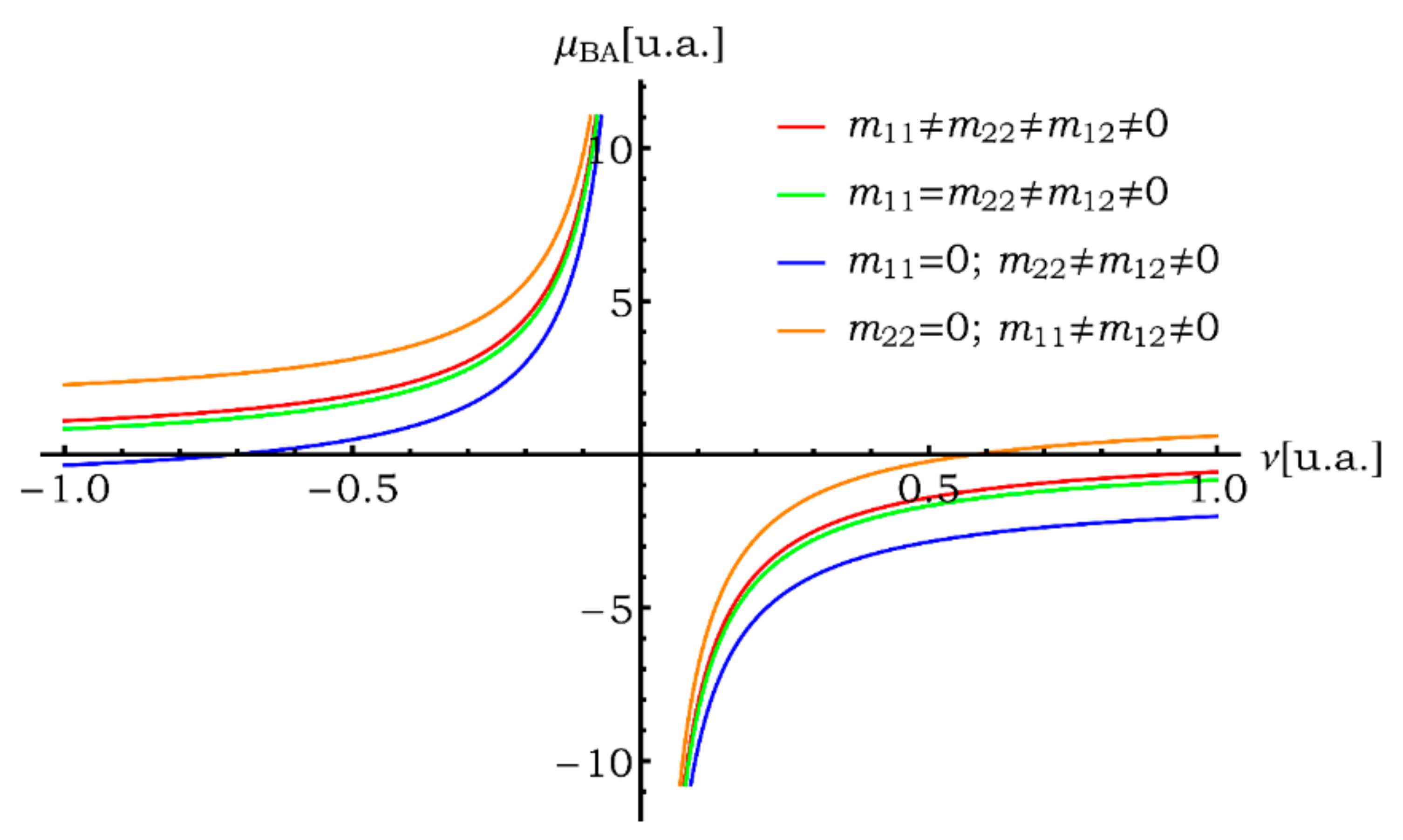
We observe in Figure 3 that the dipole moment in the adiabatic basis has hyperbolic characteristics with clear divergences for zero values of the coupling parameter. However, it is necessary to point out that this transition dipole makes physical sense by incorporating intramolecular effects. According to the coupling parameter, the behavior is not very sensitive to the cases of nullity of the permanent dipoles or equality between them.

We note in Figure 4a, that at weak pumping beam perturbations, expressed in terms of the Rabi saturation frequency ${\mathsf{\Omega }}_1$, the intensity of the emerging beam of the FWM signal varies little concerning the coupling parameter. However, when the pumping intensity is raised to the value 1 (a.u), not only does the emerging signal intensity increase considerably, but the inversely increasing sensitivity with the value of the coupling parameter is distinguished in it. From Equation (70), we observe that the FWM signal intensity, normalized with respect to the intensity value of the test beam, has explicit dependence both on the optical length and with the $\Delta {\mathrm{k}}_{\mathrm{z}}$ detuning, while it maintains an implicit dependence with the structure details governed by the coupling parameter. In Equation (70) it is observed that, as the absorption of the FWM beam as it passes through the optical length becomes smaller, the signal intensity increases. The latter refers to the crossing of curves and the weakening of the transition intensity due to its diagonal character between the adiabatic states, unlike what could occur in a system of two diabatic states, where the transition occurs vertically without changes in the nuclear coordinate. It is important to note that in Equation (70), it is possible to show that the intensity of the coupling process ${\left|{\mathsf{\xi }}_3(0)\right|}^2$ is less than the square of the detuning $\Delta {\mathrm{k}}_{\mathrm{z}}\approx 2{\mathrm{k}}_{1\mathrm{z}}-{\mathrm{k}}_{2\mathrm{z}}-{\mathrm{k}}_{3\mathrm{z}}$ (see Equation (63)). In Figure 4b, we extend the result to observe the topological behavior of the FWM signal concerning different values of coupling and saturation of part of the pumping beam. We note that the intensity of the emerging signal along the optical path becomes higher only at low values of the intramolecular coupling and high intensity of the pump beam. In the latter, the saturation effect, in interaction with the molecular system, causes networks of populations, and the pump beam itself is dispersed.

It should be noted that the Rabi frequency of the pumping beam has an implicit dependence on the coupling parameter, since the transition dipole moment chosen for the radiation-matter interaction is calculated on the adiabatic representation associated with the $\left|\mathrm{A}\right.〉$ and $\left|\mathrm{B}\right.〉$ states. It is also important to note that the terms related to the pump-probe coupling processes given by ${\left|{\mathsf{\xi }}_3(0)\right|}^2$ are taken at the optical propagation origin because their change in optical length is very low. We selected an internal angle between the pump and probe incident beams, of the order of of $\mathsf{\sigma }=3°$ (0.0523599 radians), given the very fast decay of the FWM signal intensity as the optical length increases, and according to the sin functions, such as the J-Bessell functions. We observe from Figure 4a,b, that the dependence of the intensity of the emerging FWM signal on the intensity of the pumping beam is greater than the linearity, which leads us to suppose that there is a slight parametric amplification at these values of optical length and vibronic coupling, tunable with the organic dye Malachite green chloride used in our calculations [48].

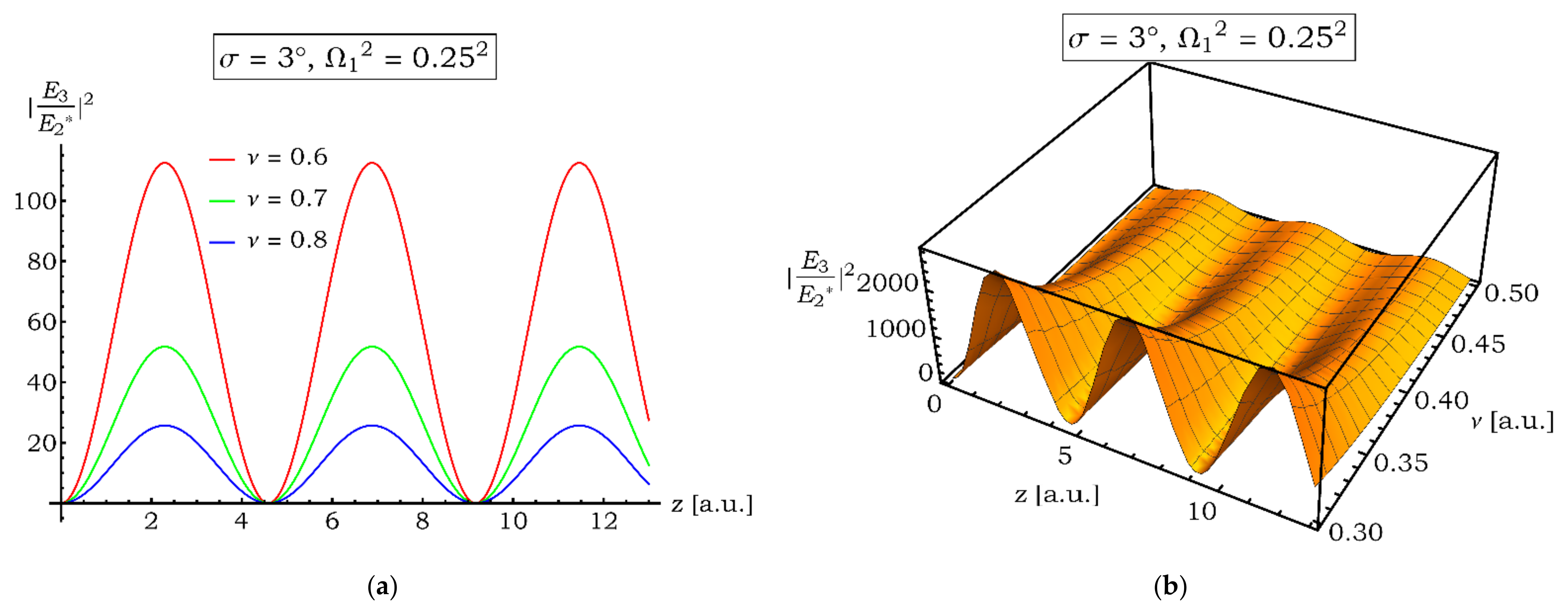
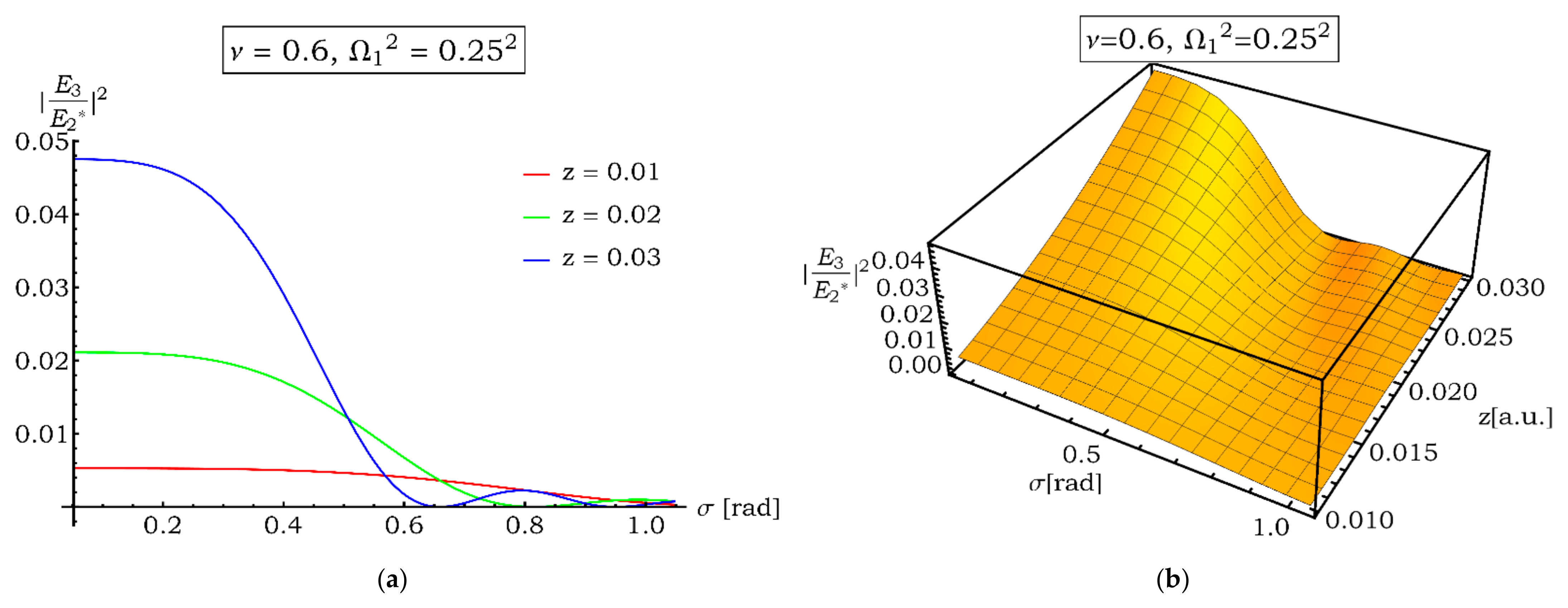
In Figure 5a, we can observe that the FWM signal intensity, as it progresses in optical length, has a periodic pattern whose minima and maxima maintain a localized separation at z. We observe the decrease of intensity within the period as we increase the vibronic coupling parameter. This pattern of behavior can be demonstrated from Equation (70). In Figure 5b, we extend the study for other vibronic coupling parameter values and different optical length values. We observe the generalized behavior of decreasing signal intensity as the vibronic coupling parameter increases because of reducing effective absorption of the pumping and probe beams.

Here, in Figure 6a, we observe that the emerging FWM signal increases in intensity as more energy increases in the pump-test coupling process. It is important to note that the pattern of decreasing signal intensity is repeated in each cycle of this periodic system. We extend the analysis through Figure 6b for longer optical length and pumping beam intensity behaviors. The analysis is carried out keeping the incident angle value at this optimum value and vibronic coupling parameter equal to 0.6. We choose this small value of $\mathsf{\nu }$ to specify that the behavior of the FWM signal maintains the periodic behavior established in Equation (70).

In the above equation, the square module of the ratio of electric field amplitudes is given. This ratio depends upon many factors; in particular, it depends on z. When the ratio of these amplitudes is plotted against z, for different coupling factors, as shown in Figure 4 and, for different Rabi frequencies, as shown in Figure 5, it gives an oscillatory behavior. In these graphics, we see that the frequency of this oscillatory behavior is independent of the values of $\mathsf{\nu }$ and ${\mathsf{\Omega }}_1^2$. Furthermore, we set to zero the derivative of Equation (70) concerning z and found an analytical condition for extremes. Indeed, the ratio of amplitudes has an extreme value whenever requirement (66) is fulfilled.

$$\mathrm{z}=\mathrm{n}\frac{\mathsf{\pi }}{1000\left|1-\cos \mathsf{\sigma }\right|}$$

(71)

where n is an integer. If n is odd, there is a maximum, and if it is even, there is a minimum. The condition shown in Equation (71) depends only on the angle, $\mathsf{\sigma }$, between the wave vectors ${\overrightarrow{\mathrm{k}}}_1$ and ${\overrightarrow{\mathrm{k}}}_2$. There is no dependence upon $\mathsf{\nu }$ nor ${\mathsf{\Omega }}_1^2$, as expected from Figure 4 and Figure 5. For instance, when $\mathsf{\sigma }=3°$ maximums are found at $\mathrm{z}=2.29,6.88,11.46$, etc., and minimums are found at $\mathrm{z}=0.4,4.58,9.17$, etc. In other words, through Equation (70) it is possible to establish the periodic pattern shown by the FWM signal along the optical length as a function of both the intensity of the incident pump and in terms of the intramolecular coupling.

In this curve, we appreciate that the FWM signal intensity has less than 0.6 radians higher values as the optical length is greater. This is seen when we keep within a stable cycle. For the selected values, and compared with Figure 5a, at values of $\mathsf{\nu }=0.6$ the signal grows in intensity. However, when we propagate the signal along the optical length, we observe a decay as the pump-probe incidence angle becomes larger, demonstrating that the $\Delta {\mathrm{k}}_{\mathrm{z}}$ detuning becomes smaller as the angle becomes smaller. The continuous bouncing is a consequence of the dependence of the FWM signal intensity on this detuning through the $\mathsf{\theta }=\Delta {\mathrm{k}}_{\mathrm{z}}\mathrm{z}/2$ magnitude defined above.

In Figure 7, we extend our results of normalized FWM signal behavior as a function of optical length and incidence angles between the pumping and probe beams. We observe that at sigma values close to the optimal value of $\sim 0.0524$ radians, the FWM signal intensity has a maximum for the selected value of z. We select a saturation value of ${(0.25)}^2$ and a fixed value of the intramolecular coupling parameter. We note, however, that the maximum intensity value is reached for spatial $\Delta {\mathrm{k}}_{\mathrm{z}}$ detuning values close to zero. Experimentally, being in this near-zero detuning regime prevents separation of the generated FWM signal from the incident beams correctly. Moreover, locating the signal of very low intensity, compared to the strong intensity of the pumping, both penetrating almost in the same region, would make the experiment very complicated to perform.

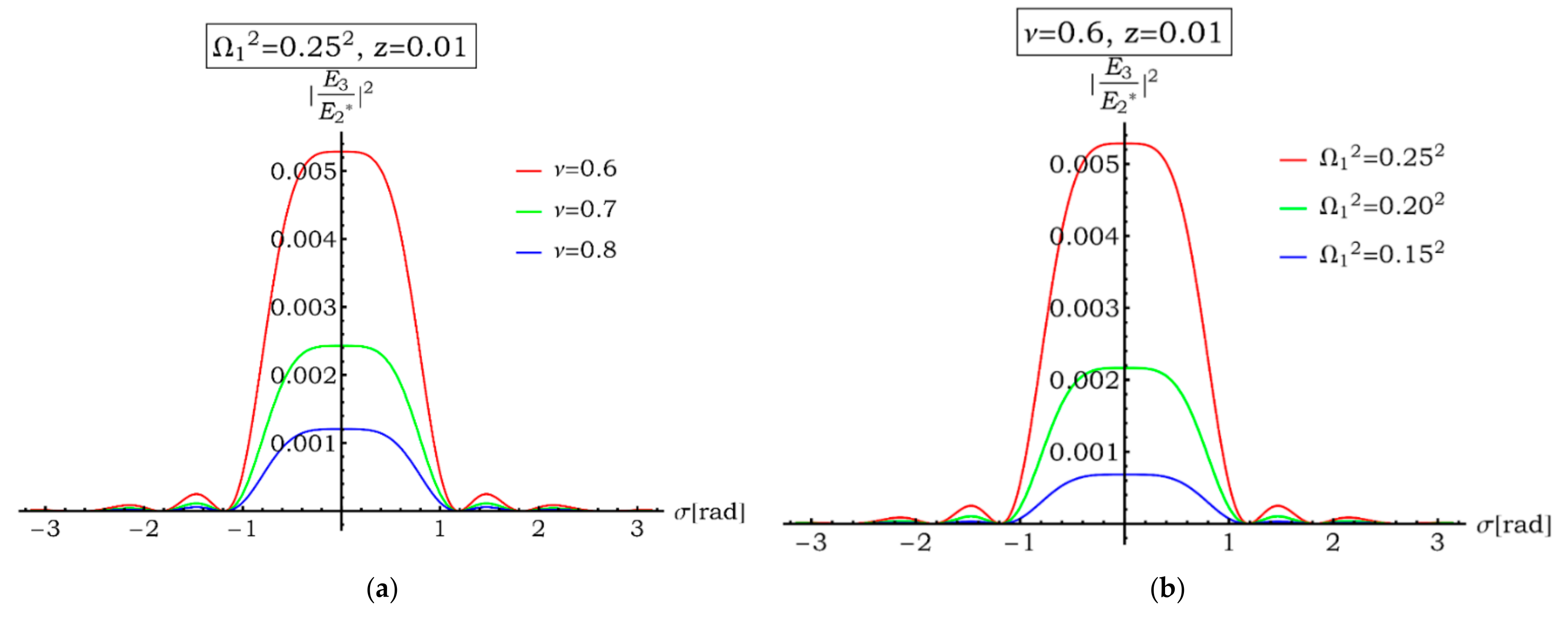
We observe how the bounce of the FWM signal as the angle of incidence persists, regardless of whether we vary the coupling parameter (Figure 8a) or the value of the saturation intensity of the pumping beam (Figure 8b). This assertion is possible according to Equation (70) where we can see that the decay pattern is very similar to the J-Bessell function, and where we can see that for incidence angles greater than 1, the signal practically disappears. However, it is convenient to point out the convenience of working with very low coupling parameters and very high pumping intensities for a higher resolution of the FWM signal.

4. Conclusions

In this investigation, we have developed a radiation-matter interaction model considering a two-state system and a model molecule which consists of two coupled harmonic curves of electron energy shifted in both the energy and the nuclear coordinates. We have also considered two vibrational states, and we have included non-adiabatic effects for this two-state model. By developing a semi-classical model and making use of conventional optical Bloch equations for the density matrix of the subsystem under study, we calculated the nonlinear macroscopic polarizations corresponding to each of the representative fields of the nondegenerate FWM signal. We studied the signal propagation effects under the influence of the saturation effects of the incident pumping field and in the presence of intramolecular effects. We have derived an effective transverse relaxation time ${\tilde{\mathrm{T}}}_2$ instead of ${\mathrm{T}}_2$, to include the effect of intramolecular coupling in the model. It is important to point out that the use of this new adiabatic basis, generated by the effects of the residual spin-orbit Hamiltonian, allows us to define new dipole moments, considered as critical quantities in our analysis. Finally, propagation studies indicated that, within the optical length of study, the FWM signal shows a periodic structure in its behavior, with localized maxima and minima, coinciding with known experimental results or with models proposed by other authors [40,49]. The reported amplification shows that the process is tunable through the organic dye used as a subsystem of study.