Developing an EFDC and Numerical Source-Apportionment Model for Nitrogen and Phosphorus Contribution Analysis in a Lake Basin

Abstract

The numerical source-apportionment model is an efficient and useful method for analyzing water-quality responses to nutrient loading in rivers and lakes. In this study, the Environmental Fluid Dynamic Code (EFDC) and numerical source-apportionment model were applied to Lake Bali in Jiujiang City, China to predict the contributions of various pollution sources to the lake at any time and position. We calibrated and validated the model by comparing its predictions with observed hydrodynamic and water-quality parameters from 2014 to 2015. Application of the calibrated model to simulate water-quality responses to a pollution source showed that the contribution of a pollution source to water quality in the lake has strong spatial heterogeneity. The results provide useful information for the optimization of pollution load reduction in Lake Bali and can be used to determine the most effective implementation of its pollution-control plan. The model built in this study can also be used for pollution source-apportionment in other urban lakes and is superior to other traditional source-apportionment models.

1. Introduction

Meticulous management and control of watersheds based on water-quality targets has become a primary interest of water environment managers in China. The source-apportionment method can be used to establish the input response relationship between pollution sources and water quality and to quantitatively calculate their relationship across different spatiotemporal scales in the basin. The source-apportionment method generally includes both an experimental and a modeling component. The experimental method is based on carbon isotope analysis of a specific pollutant [1,2,3]. However, the receptor model, which includes the grey box model, a statistical model, and a numerical model, is most commonly used in water environmental management. Chemical mass balance is the most representative source-apportionment method based on the grey box model [4], which considers mass conservation and assumes that there is no reaction between pollutants, that the quantities of pollutants in the water are equal to the linear sum of contributions from various sources, and that the contribution of each pollution source remains steady. However, this method has strong limitations in practical application and its basic assumptions are difficult to support in more complicated cases because it can neither distinguish pollution sources at different times nor calculate the contribution of each pollution source to the water quality at different locations [2].

Another source-apportionment method based on statistical modeling calculates the proportion of pollutants in the water coming from pollution sources using the relationship between substances in statistical and monitoring data, including factor analyses [5,6,7], principal component analyses [8,9,10], cluster analyses [11,12,13,14,15], and multiple linear regression. This led to the hypothesis that there is no significant change in the composition of pollutants from generation to acceptor and that individual pollutant flux is proportional to pollutant concentration [16]. These assumptions are not valid in large systems, and the mechanisms behind them have not been established, which makes it difficult to obtain satisfactory and useful results. Due to the limitations of the grey box and statistical models, the direct contributions of different sources in time and space cannot be effectively identified. The source-apportionment method, which is based on a numerical model, has attracted attention in recent years because it follows the energy conservation theorem and has high spatiotemporal resolution.

Currently, most research uses a simpler numerical model or a numerical model combined with the methods mentioned above [17,18,19]. The simple numerical model can produce the results of source-apportionment analysis, but because the simple model itself has the problems of over-fitting, low spatiotemporal resolution, and a lack of natural mechanism, numerical source apportionment, which is useful for practical management, is based on a distributed or semi-distributed model, such as the Soil Water Assessment Tool (SWAT), Agricultural Non-Point Source Pollution Model, etc. Alternately, source apportionment is often combined with statistical analysis where the source contribution is obtained by short time model operation. The analytical difficulty of this method is that it determines the source type and characteristics [20]. In addition, statistical analyses only include a source-apportionment result for a specific time frame (such as the annual mean) or a space scale, and the spatiotemporal heterogeneity of the pollution characteristics cannot be fully explored.

In summary, the abovementioned source-apportionment methods are not able to provide effective technical support for careful management and control of watersheds based on water-quality targets. Therefore, using the water-quality input response relationship, we constructed a spatiotemporal numerical source-apportionment model for use in Lake Bali based on the Environmental Fluid Dynamics Code (EFDC), which is widely used in water-quality simulations [21,22,23,24]. By running the model once, we were able to calculate the contribution of a pollutant source at any time or position. This not only solves the efficiency problem of repeated computation of the traditional numerical source-apportionment method, but also provides a more scientific and effective method for decision-making in management departments.

2. Materials and Methods

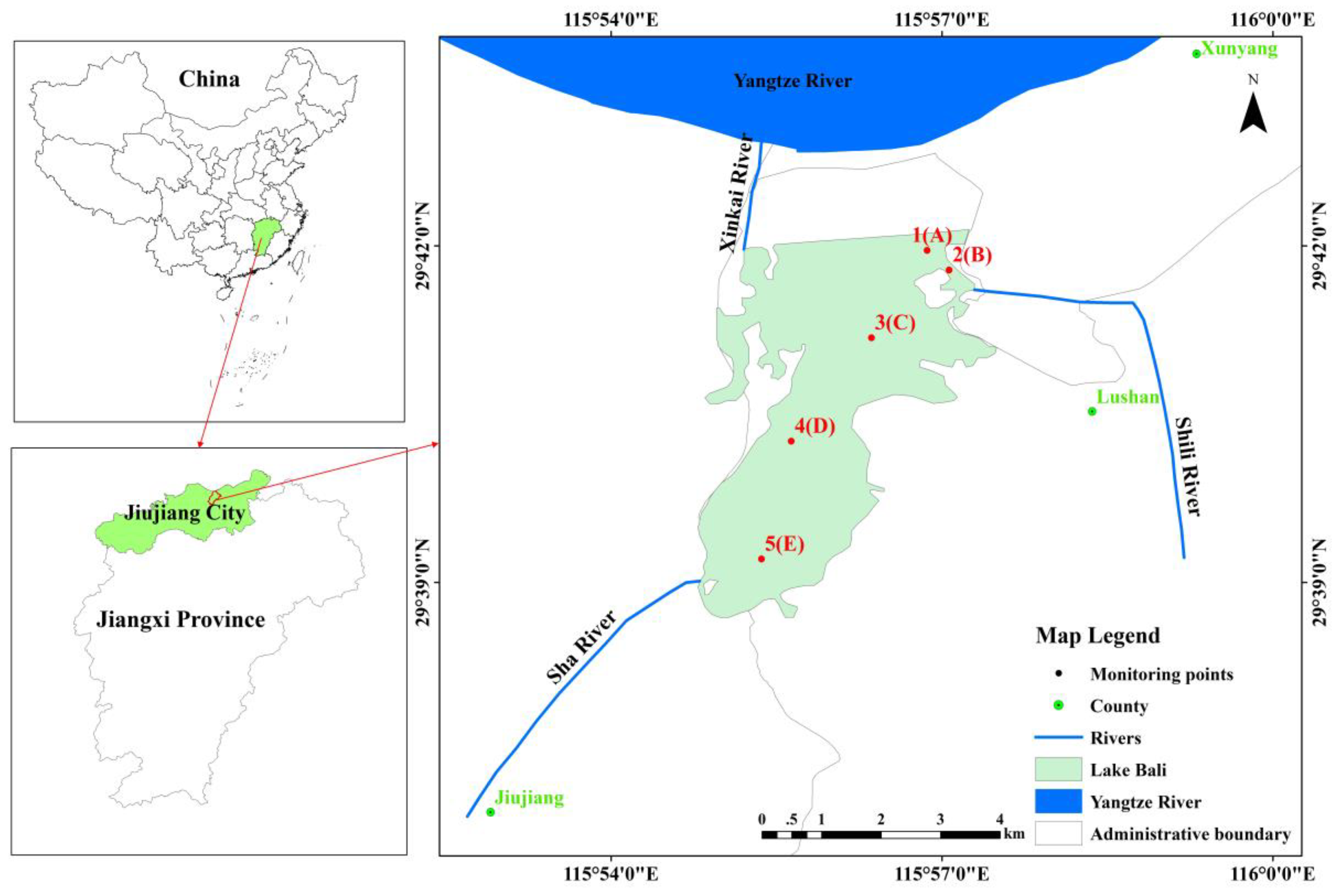
2.1. Study Area

Lake Bali is a small lake in Jiujiang City, Jiangxi Province that is located to the west of the city center and is adjacent to Lushan Mountain. It connects to the Yangtze River by a water gate in the Xinkai River. The surface area of the lake is 18 km², with a corresponding storage of 1.54 × 10⁸ m³, and average depth of 3.69 m (at a water level of 18.97 m). The basin contains Lake Bali, the Shili River, the Sha River, and the Xinkai River, and drains a catchment area of 200 km² (Figure 1). The lake was selected from a good lake protection list in China, and had a water-quality target of surface water-quality standard Class III. The main pollutants in the lake are nitrogen and phosphorus, and the water is facing an increasing risk of eutrophication. As the urban area of Jiujiang City expands, future development of the city may further increase pressure on the lake’s water-quality improvement. Thus, an analysis of the sources and contributions of nitrogen and phosphorus in Lake Bali, based on which countermeasures to pollution could be made, is urgently required to improve water quality.

2.2. Model Description

EFDC is a general-purpose modeling package for simulating one-, two-, and three-dimensional flow, transport, and bio-geochemical processes in surface water systems, initially developed at the Virginia Institute of Marine Science [25,26]. The model has been extensively applied to simulate circulation, thermal stratification, sediment transport, water quality, and eutrophication processes in numerous lakes, rivers, reservoirs, wetlands, and estuaries [21,22,23,24,27,28,29,30,31,32].

In the current study, a total nitrogen (TN) and total phosphorus (TP) source-apportionment model of Lake Bali was built in EFDC. This model can be used to calculate the contribution of any pollution source to the lake at any time and location. We first, derived a set of partial differential equations by taking the partial derivative of water quality with respect to each pollution source. Second, we solved these differential equations to quantify the contribution of each pollution source. Finally, by running the model only one time, we directly calculated the contribution of each pollution source at each spatial and temporal point in the lake.

2.2.1. Hydrodynamic Water-Quality Model in EFDC

(1) Hydrodynamic Model

Because the hydrodynamic model in EFDC is based on three-dimensional hydrostatic equations formulated in curvilinear, orthogonal, and horizontal coordinates and a sigma vertical coordinate, it can be applied to one-dimensional and two-dimensional cases without modifying the code. In this study, we used two-dimensional hydrostatic equations. The hydrodynamic model describes the hydrological characteristics and flow field in the water body. It includes momentum and continuity equations and transport equations for turbulence, salinity, temperature, and sediment. A detailed description of the hydrodynamic module is available from Hamrick [25] and Craig [33].

(2) Water-Quality Model

The water-quality model in EFDC solves the mass–balance equations of 22 constituents in the water column, including algal groups, organic carbon cycles, phosphorus, nitrogen, silica, dissolved oxygen, and fecal coliform bacteria [34,35]. In this study, we simulated TN and TP fate and transport. The water-quality module includes sedimentation and first-order degradation. The mass–balance equation for the water-quality constituents is [25,26]:

$$\begin{array}{l}\frac{\partial }{\partial t}(m_x{m}_{y}HC)+\frac{\partial }{\partial x}(m_{y}HuC)+\frac{\partial }{\partial y}(m_{x}HvC)+\frac{\partial }{\partial z}(m_x{m}_{y}wC)=\\ \frac{\partial }{\partial x}(\frac{m_{y}H{A}_x}{m_x}\frac{\partial C}{\partial x})+\frac{\partial }{\partial y}(\frac{m_{x}H{A}_y}{m_y}\frac{\partial C}{\partial y})+\frac{\partial }{\partial z}(m_x{m}_y\frac{A_z}{H}\frac{\partial C}{\partial z})+m_x{m}_y{W}_s\frac{\partial C}{\partial z}+S_c\end{array}$$

(1)

where C is the water concentration; u, v, and w are the velocity components in the x, y, and z directions in curvilinear orthogonal coordinates, respectively; A_x, A_y, and A_z are the diffusion coefficients in the x, y, and z directions; W_s is the coefficient of material deposition (m⁻¹); S_c is the first-order degradation rate that acts as a source or sink; H is the water depth (m); m_x and m_y are the scale factors of plane curvilinear coordinates; and t is time.

In Equation (1), the last three items on the left side express convective transport, and the first three items on the right side express diffusion transport and settling. The last item on the right side represents the degradation process and exogenous load, which is

$$S_c=-m_x{m}_{y}HKC+{\displaystyle \sum _{i=1}^N{P}_i}$$

(2)

where K is the degradation coefficient (day⁻¹) and P_i is the load for substance J (kg/day); i is an index from 1 to N.

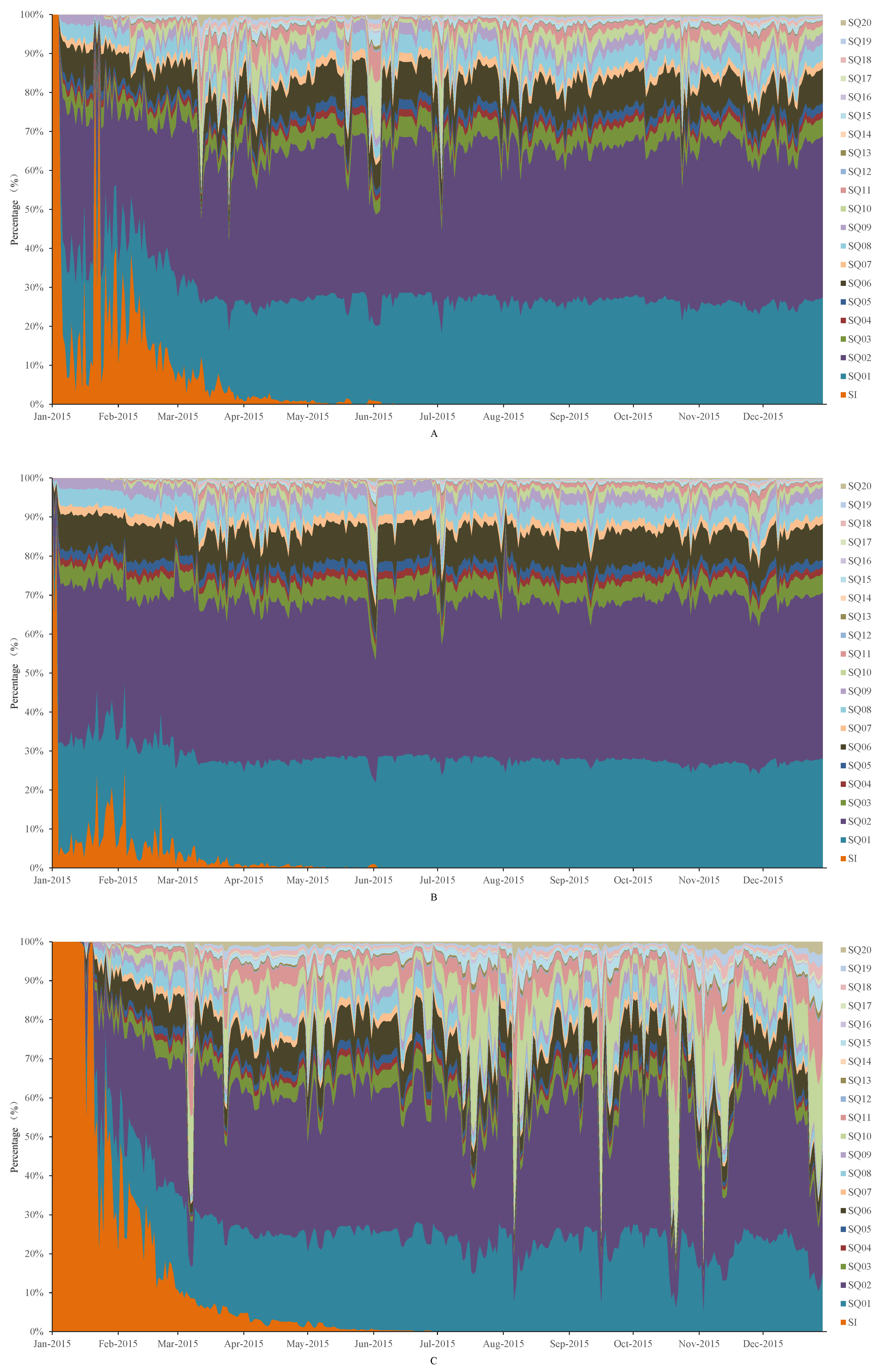
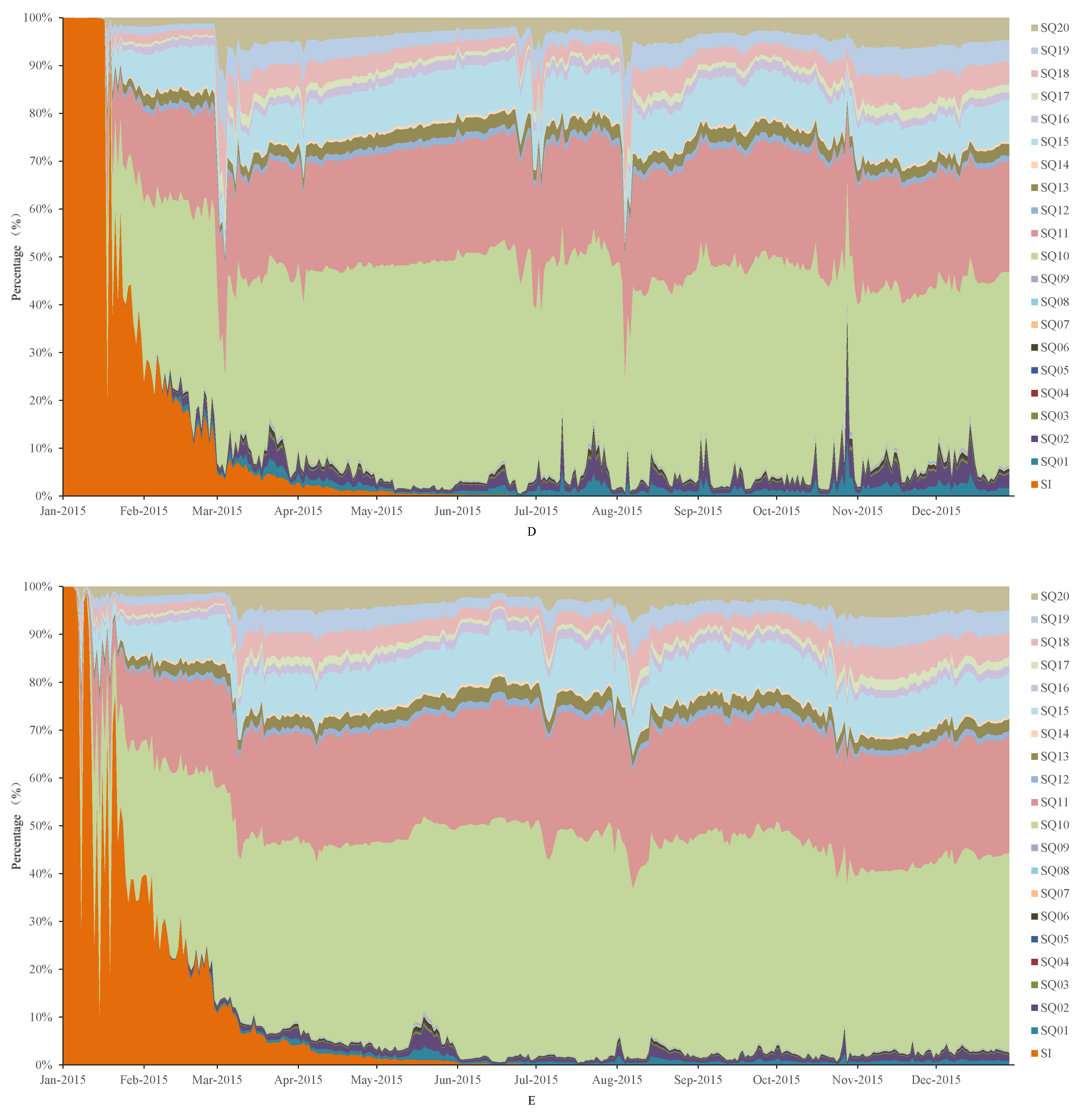
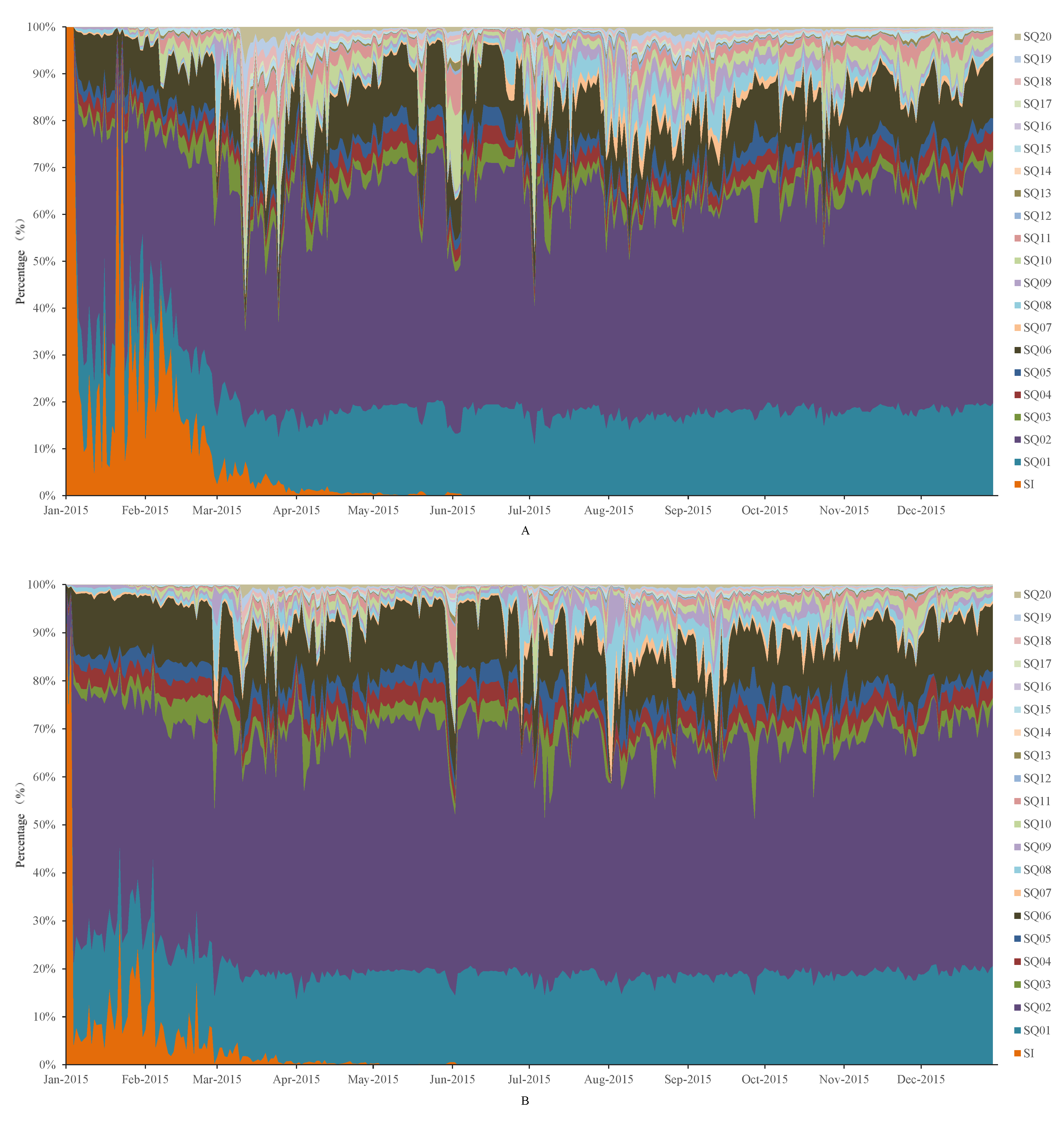
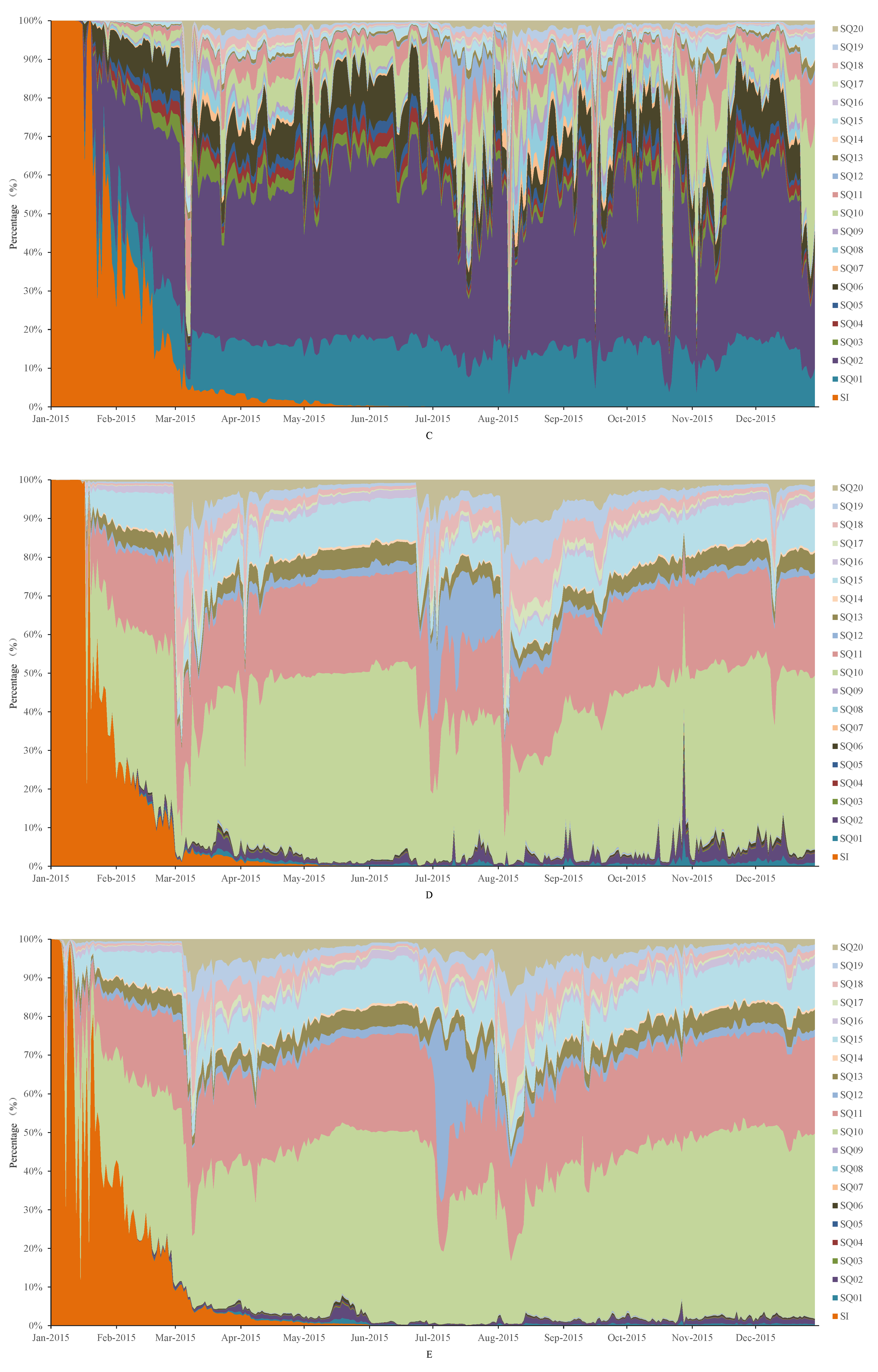
2.2.2. Numerical Source-Apportionment Model

The formula $S_I=\frac{\partial C}{\partial C_0}$ represents the contribution of background concentration to simulated water quality by applying the chain rule to (1):

$$\begin{array}{l}\frac{\partial }{\partial t}(m_x{m}_{y}H{S}_I)=-\frac{\partial }{\partial x}(m_{y}Hu{S}_I)-\frac{\partial }{\partial y}(m_{x}Hv{S}_I)-\frac{\partial }{\partial z}(m_x{m}_{y}w{S}_I)\\ +\frac{\partial }{\partial x}(\frac{m_{y}H{A}_x}{m_x}\frac{\partial S_I}{\partial x})+\frac{\partial }{\partial y}(\frac{m_{x}H{A}_y}{m_y}\frac{\partial S_I}{\partial y})+\frac{\partial }{\partial z}(m_x{m}_y\frac{A_z}{H}\frac{\partial S_I}{\partial z})\\ +m_x{m}_y{W}_s\frac{\partial S_I}{\partial z}-m_x{m}_{y}HK{S}_I\end{array}$$

(3)

Similarly, $S_i=\frac{\partial C}{\partial P_i}$ represents the contribution of a pollution source to simulated water quality,

$$\begin{array}{l}\frac{\partial }{\partial t}(m_x{m}_{y}H{S}_i)=-\frac{\partial }{\partial x}(m_{y}Hu{S}_i)-\frac{\partial }{\partial y}(m_{x}Hv{S}_i)-\frac{\partial }{\partial z}(m_x{m}_{y}w{S}_i)\\ +\frac{\partial }{\partial x}(\frac{m_{y}H{A}_x}{m_x}\frac{\partial S_i}{\partial x})+\frac{\partial }{\partial y}(\frac{m_{x}H{A}_y}{m_y}\frac{\partial S_i}{\partial y})+\frac{\partial }{\partial z}(m_x{m}_y\frac{A_z}{H}\frac{\partial S_i}{\partial z})\\ +m_x{m}_y{W}_s\frac{\partial S_i}{\partial z}-m_x{m}_{y}K{S}_i+P_i\end{array}$$

(4)

To deal with large potential parameter sensitivities, we introduced parameter perturbation to replace the sensitivity. We defined parameter k, with perturbation $r=dk/k$,

$$\frac{\partial C}{\partial \mathrm{k}}=\frac{\partial C}{\mathrm{k}\partial r}=\frac{1}{\mathrm{k}}\frac{\partial C}{\partial r}$$

(5)

The preceding was introduced into (3) and (4) using $S_I^{\prime }$ and $S_{\mathrm{i}}^{\prime }$ to represent the contributions of the pollution source to the water quality,

$$\begin{array}{l}\frac{\partial }{\partial t}(m_x{m}_{y}H{S}_I^{\prime })=-\frac{\partial }{\partial x}(m_{y}Hu{S}_I^{\prime })-\frac{\partial }{\partial y}(m_{x}Hv{S}_I^{\prime })-\frac{\partial }{\partial z}(m_x{m}_{y}w{S}_I^{\prime })\\ +\frac{\partial }{\partial x}(\frac{m_{y}H{A}_x}{m_x}\frac{\partial S_I^{\prime }}{\partial x})+\frac{\partial }{\partial y}(\frac{m_{x}H{A}_y}{m_y}\frac{\partial S_I^{\prime }}{\partial y})+\frac{\partial }{\partial z}(m_x{m}_y\frac{A_z}{H}\frac{\partial S_I^{\prime }}{\partial z})\\ +m_x{m}_y{W}_s\frac{\partial S_I^{\prime }}{\partial z}-m_x{m}_{y}HK{S}_I^{\prime }\end{array}$$

(6)

$$\begin{array}{l}\frac{\partial }{\partial t}(m_x{m}_{y}H{S}_{{}_i}^{\prime })=-\frac{\partial }{\partial x}(m_{y}Hu{S}_{{}_i}^{\prime })-\frac{\partial }{\partial y}(m_{x}Hv{S}_{{}_i}^{\prime })-\frac{\partial }{\partial z}(m_x{m}_{y}w{S}_{{}_i}^{\prime })\\ +\frac{\partial }{\partial x}(\frac{m_{y}H{A}_x}{m_x}\frac{\partial S_{{}_i}^{\prime }}{\partial x})+\frac{\partial }{\partial y}(\frac{m_{x}H{A}_y}{m_y}\frac{\partial S_{{}_i}^{\prime }}{\partial y})+\frac{\partial }{\partial z}(m_x{m}_y\frac{A_z}{H}\frac{\partial S_{{}_i}^{\prime }}{\partial z})\\ +m_x{m}_y{W}_s\frac{\partial S_{{}_i}^{\prime }}{\partial z}-m_x{m}_{y}K{S}_{{}_i}^{\prime }+P_i\end{array}$$

(7)

2.2.3. Solution of the Source-Appointment Model

The numerical solution to the source-appointment equation is the same as that of the water-quality equation. We separately determined the sedimentation, degradation, source/sink and convection, and diffusion contributions to water quality with mass–balance equations.

The mass–balance equation for convection and diffusion is:

$$\begin{array}{l}\frac{\partial }{\partial t}(m_x{m}_{y}HC)=-\frac{\partial }{\partial x}(m_{y}HuC)-\frac{\partial }{\partial y}(m_{x}HvC)-\frac{\partial }{\partial z}(m_x{m}_{y}wC)\\ \frac{\partial }{\partial x}(\frac{m_{y}H{A}_x}{m_x}\frac{\partial C}{\partial x})+\frac{\partial }{\partial y}(\frac{m_{x}H{A}_y}{m_y}\frac{\partial C}{\partial y})+\frac{\partial }{\partial z}(m_x{m}_y\frac{A_z}{H}\frac{\partial C}{\partial z})\end{array}$$

(8)

The mass–balance equation for sedimentation, degradation, and source/sink is:

$$\frac{\partial }{\partial t}(m_x{m}_{y}HC)=-m_x{m}_y{W}_s\frac{\partial C}{\partial z}-m_x{m}_{y}HKC+{\displaystyle \sum _{i=1}^N{P}_j}$$

(9)

The solution to the mass–balance equation for convection and diffusion is the same as the material-balance equation for salt in the hydrodynamic model. Equations (8) and (9) are solved with second-order accuracy and a three-time level algorithm.

The first step was to solve the sedimentation, degradation, and source/sink terms during ∆t (from t_n−1 to t_n), and then $C_{-p}^n$ (the concentration of a substance at time t_n) as:

$$m_x{m}_y{H}^{n-1}{C}_{-P}^n=m_x{m}_y{H}^{n-1}{C}^{n-1}-\Delta t{m}_x{m}_{y}Ws\frac{\partial C^{n-1}}{\partial z}-\Delta t{m}_x{m}_y{H}^{n-1}K{C}^{n-1}+\Delta t{\displaystyle \sum _{i=1}^N{P}_i^{n-1}}$$

(10)

where n is the time step, and the subscript −P represents water-quality concentration in the absence of convection and diffusion during ∆t.

The subscript −K represents water-quality concentration in the absence of settling, degradation, and sources/sinks during ∆t; the subscript +K represent the water-quality concentration subject to settling, degradation, and sources/sinks during ∆t. Here, $C_{-p}^n=C_{+k}^{n-1}$.

The second step was to solve the finite-difference form of (9) from t_n−1 to t_n+1 (water-quality concentration subject to convection and diffusion during two ∆t, $C_{-p}^n$ or $C_{+k}^{n-1}$):

$$m_x{m}_y{H}^{n+1}{C}_{-K}^{n+1}=m_x{m}_y{H}^{n-1}{C}_{+K}^{n-1}+2\Delta tPT$$

(11)

In Equation (11), PT is the material migration operator during two ∆t, and $C_{-K}^{n+1}$ is water-quality concentration in the absence of settling, degradation, and sources/sinks at t_n+1.

The third step is to implicitly solve (9) as:

$$\begin{array}{l}{m}_x{m}_y{H}^{n+1}{C}_{}^{n+1}=m_x{m}_y{H}^{n+1}{C}_{+P}^n-\Delta t{m}_x{m}_{y}Ws\frac{\partial C_{+P}^n}{\partial z}-\Delta t{m}_x{m}_y{H}^{n+1}K{C}^{n+1}\\ +\Delta t{\displaystyle \sum _{i=1}^N{P}_i^{n+1}}\end{array}$$

(12)

where the subscript −P represents water-quality concentration subject to convection and diffusion, and Cⁿ⁺¹ is water-quality concentration at t_n+1.

Next, the solution from the hydrodynamic module and from (2) were combined. Equations (3) and (4) were solved using the same method. Equation (4) is a general form of an external/internal source, and each source has its own independent equation, with N sources (4) will comprise N partial differential equations. The partial differential equations for each source are solved individually, and N sources are solved simultaneously. We obtained the spatiotemporal water-quality contribution of a specific source was obtained by solving these equations.

2.3. Model Configuration

The model for Lake Bali was set up by generating a modeling grid and defining meteorological and boundary conditions. Model development was supported with key data sources. The model development steps and data used to identify boundary conditions, initial conditions, and calibration of key model parameters are discussed below.

(1) Grid Generation

The Lake Bali model comprised Lake Bali, the Shili River, the Sha River, and the Xinkai River (Figure 1). The Shili River, Sha River, and Xinkai River were connected by point sources that govern the direction of flow either into or out of Lake Bali. Model grid generation was based on a bathymetric survey of Lake Bali that was performed in July 2015. These data include bottom elevations of several locations throughout the lake. The depth-averaged model domain was discretized into a grid consisting of 2502 two-dimensional orthogonal curvilinear computational cells.

(2) Boundary Conditions

To simulate water circulation and water quality with the EFDC, the model was driven by boundary conditions including inflow from the Shili River and Sha River sub-watershed pollution sources and outflow through Xinkai River dam release in addition to atmospheric forcing. The flow rates and nutrient loading of inflows from the 20 sub-watershed pollution sources (

Table 1. Information of the 20 sub-watershed pollution sources.

Generalizability Name in the Model	Type of Pollution Source	Position
SQ01	Urban sources with concentrated discharge	Shili River sub-watershed
SQ02	Urban sources with scattered discharge	Shili River sub-watershed
SQ03	Industrial sources	Shili River sub-watershed
SQ04	Large-scale livestock sources	Shili River sub-watershed
SQ05	Rural sources I	Shili River sub-watershed
SQ06	Rural sources II	Shili River sub-watershed
SQ07	Agricultural-fertilization sources I	Shili River sub-watershed
SQ08	Agricultural-fertilization sources II	Shili River sub-watershed
SQ09	Soil background sources	Shili River sub-watershed
SQ10	Urban sources with concentrated discharge	Sha River sub-watershed
SQ11	Urban sources with scattered discharge	Sha River sub-watershed
SQ12	Industrial sources	Sha River sub-watershed
SQ13	Large-scale livestock sources	Sha River sub-watershed
SQ14	Rural sources I	Sha River sub-watershed
SQ15	Rural sources II	Sha River sub-watershed
SQ16	Rural sources III	Sha River sub-watershed
SQ17	Agricultural-fertilization sources I	Sha River sub-watershed
SQ18	Agricultural-fertilization sources II	Sha River sub-watershed
SQ19	Agricultural-fertilization sources III	Sha River sub-watershed
SQ20	Soil background sources	Sha River sub-watershed

) were obtained by SWAT simulation, directly as the boundary condition of the EFDC hydrodynamic water-quality model. The EFDC grid cells that receive flow and nutrient loading from different sub-watersheds were determined based on the Shili River and Sha River estuaries. The rate of outflow was monitored by the dam flowmeter. Atmospheric forcing included hourly air pressure, air temperature, relative humidity, rainfall, evaporation, radiation, cloud cover, wind speed, and wind direction.

(3) Initial Conditions

In hydrodynamic and water-quality modeling, the initial conditions provide a starting point for the model to progress through time. We adopted an iterative approach to derive the initial condition, which used the end of year simulated condition as the initial condition for the next calibration iteration. Using this approach, the initial condition will gradually converge to a condition that reflects the complex interaction in the calibrated model. The initial water and sediment temperatures were 21 °C and 10 °C, respectively. The initial background concentrations of TN and TP in the lake were 1.5 mg/L and 0.15 mg/L, respectively, and the TN and TP concentrations in the sediment were 1.17 × 10³ mg/kg and 1.2 × 10³ mg/kg, respectively. The model ran with a start time of 1 January 2013, 10 s time step, and end time of 31 December 2015.

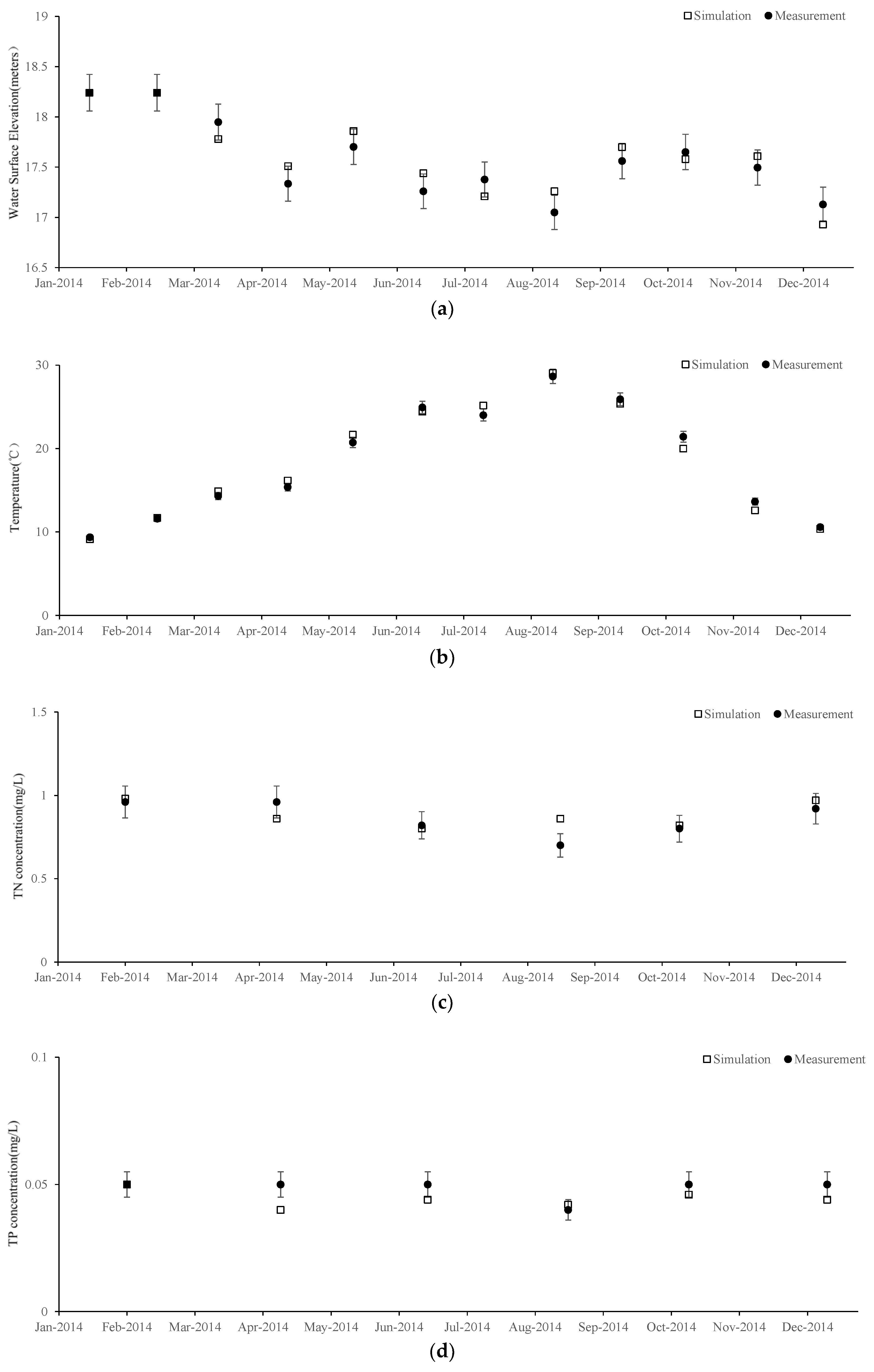
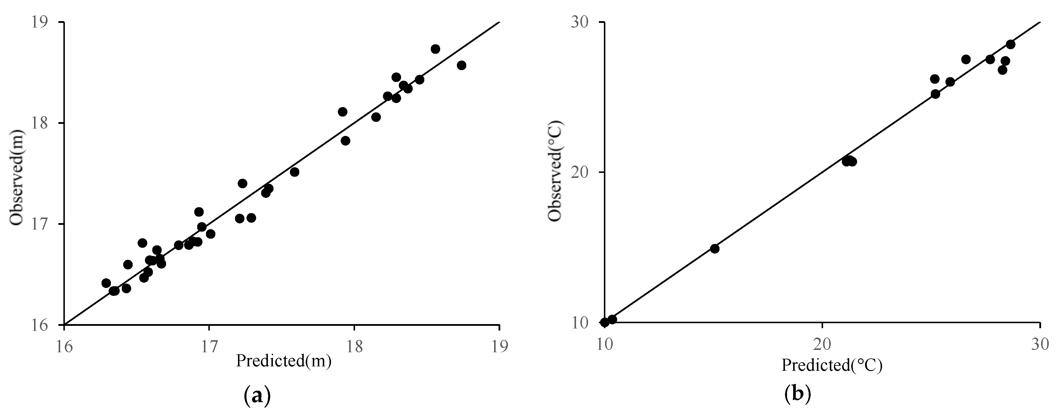
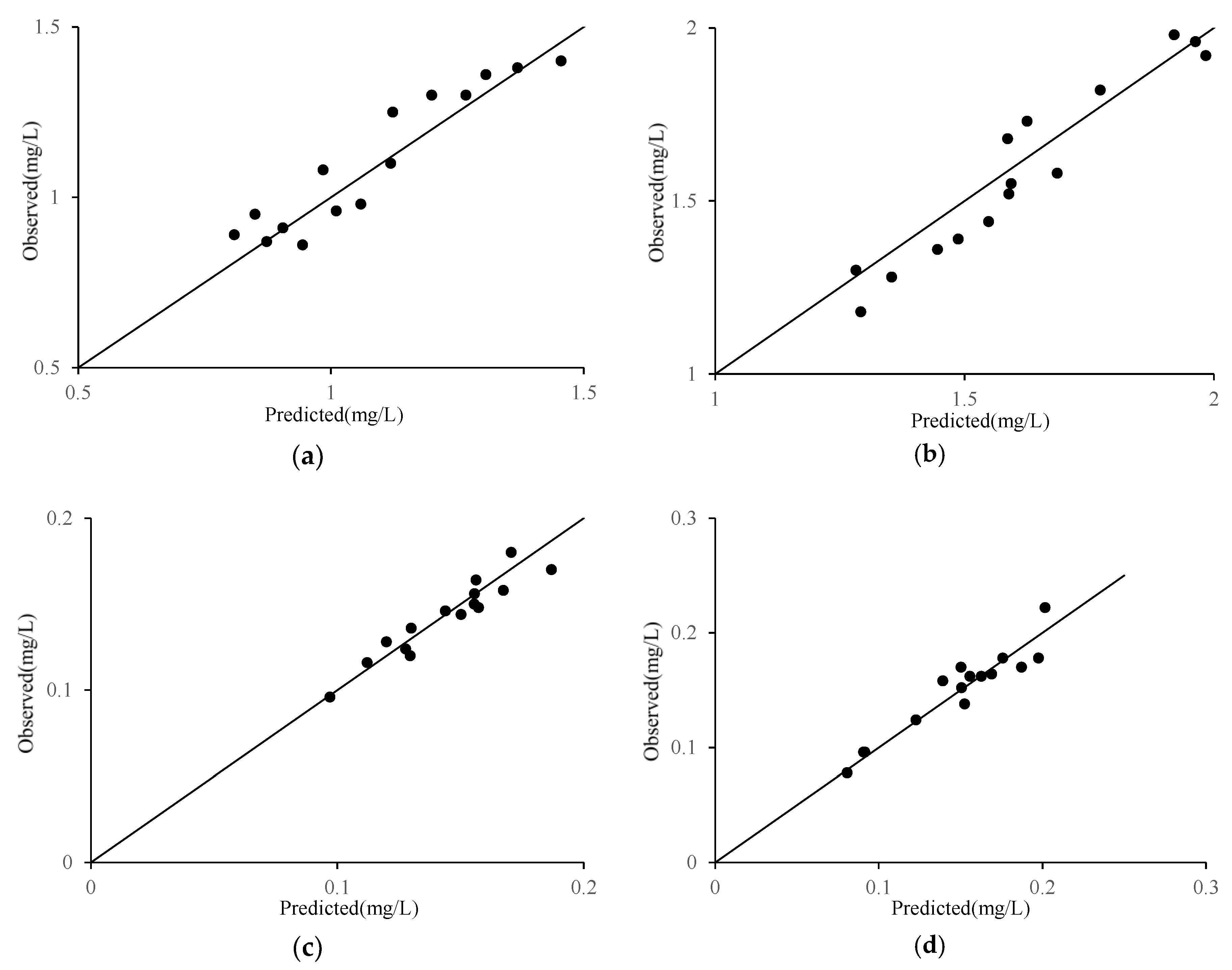
3. Model Calibration and Validation

In this study, water-quality measurements at two monitoring points (point B and point C in Figure 1), the daily water-surface elevations and water temperature at one monitoring station (Point C) from 1 January 2014 to 1 December 2014 were used to calibrate the model. Water-quality data were collected by local environmental protection monitoring. Water-surface elevation and water temperature data were collected by the local hydrological bureau. The main calibrated parameters for the model included horizontal and vertical eddy viscosities and diffusivities, degradation rate, and sedimentation rate. The EFDC model was a mature application for hydrodynamic simulation. Most of the physical parameters were not changed except for some major hydrodynamic and water-quality parameters [36]. The mean relative errors of water-surface elevation, temperature, TN, and TP at point C were 0.8%, 3.7%, 7.6%, and 9.5%, respectively (Figure 2). The calibration results showed that the simulation values agreed well with the observations.

Table 2. Main parameters of the hydrodynamic water-quality model.

Parameter	Definition	Value
AVO	Background, Constant or Molecular Kinematic Viscosity (m2/s)	1 × 10−6
ABO	Background, Constant or Molecular Diffusivity (m2/s)	1.4 × 10−9
AVMN	Minimum Kinematic Eddy Viscosity (m2/s)	1 × 10−6
ABMN	Minimum Eddy Diffusivity (m2/s)	1.4 × 10−8
KD	First-Order Degradation Rate (/d)	0.03 (TN), 0.02 (TP)
KS	Sedimentation Rate (m/d)	0.02 (TN), 0.08 (TP)

presents a summary of the main parameters in the hydrodynamic water-quality calibration.

Validation of the calibrated model was accomplished with a comparison of the simulation to measurements from 1 January 2015 to 1 December 2015. The mean relative error was used to assess the performance of the model. The mean relative errors of water-surface elevation and temperature were 0.7% and 2.3%, respectively. The scatter plots of observations vs. predictions for water-surface elevations and water temperature at points C were presented in Figure 3, showing that the simulated values agree well with the measured values. The correlation R² reached 0.9. The EFDC hydrodynamic calibration and validation results suggest that the model adequately simulates the propagation of water input into and out of Lake Bali.

We also compared the TN and TP of the model-generated results and the observed data at two monitoring sections (point C and point B). The mean relative errors of TN and TP concentrations between the observations and simulation were 8.8% and 8.1%, respectively. The scatter plots of observations vs. predictions for TN and TP at points C and point B (Figure 4), showed that most of the monitored values were in accordance with the simulated values. The correlation R² of TN and TP reached 0.8 and 0.83, respectively. The EFDC water-quality calibration and validation results suggest that the model adequately simulates the degradation process of pollutants in Lake Bali. In summary, the model can also be applied to simulate the hydrodynamic and water quality of urban lakes which are similar to Lake Bali.

4. Results and Discussion

We applied the calibrated hydrodynamic and water-quality model and source-apportionment model to calculate the source pollution contribution in Lake Bali. We selected five water-quality monitoring points to analyze the source contributions of TN and TP pollution in Lake Bali. Three of the points located in the Northern part of the lake and two were in the Southern part of the lake (Figure 1) and have been used by the environmental protection department to evaluate the overall water quality of Lake Bali. According to the reality that the pollution of Lake Bali mainly came from the input of an external load. Therefore, we did not calculate the contribution of sediment pollution. In addition, because sediment pollution treatment is expensive, and sediment removal may negatively impact lake water quality, the treatment of sediment pollution is often bypassed in the formulation and implementation of pollution source control plans. However, as is the case for many lakes undergoing eutrophication in China, water-quality impacts from sediment are significant. Therefore, it is necessary to improve the direct numerical source-apportionment model and determining how to solve this problem effectively will be the focus of future research. Here, we analyzed the contributions of industrial, urban, large-scale livestock, poultry-farm, rural, agricultural-fertilization, and soil background sources from the Sha and Shili River sub-watersheds to lake water quality by distinguishing the influence of the pollution sources.

We began by simulating the contribution of pollution sources to TN concentration at the five points over time (Figure 5). It is worth noting that the results are reliable when the impact of background concentration was eliminated. This is because the background concentration in the present study was the initial nutrient concentration in the lake, which contained a comprehensive judgement of previous contributions of different pollution sources before source apportionment.

The contributions to TN pollution at the same monitoring point varied over time, and the contributions from the different sources varied across the different monitoring points. Because the input load varies with time, the total load does not always correspond to the source-apportionment result. The contribution of TN pollution at the five points came from the background concentration of the lake at the initial time the model was run, at which time, some pollution sources had not yet reached the response point [22]. Position B is relatively sensitive, and changed first, followed by points A and C. Points E and D changed last. Overall, as the model ran, the impact of the background concentration gradually decreased. However, the impact of the background concentration on one point increased with time. This is because, with the motion of water flow around the point, the impact of background concentration around the point is much greater than that of the input load [22]. It is possible that the impact of background concentration increases when the model simulates mixing of the surrounding water. This is an advantage of the hydrodynamic water-quality model in EFDC [25,26]. As time goes on, the source contributions at some points is clear. The TN concentrations at points A, B, and C in the Northern part of the lake were mainly affected by urban sources and rural sources (SQ01, SQ02, and SQ06) that came from the Shili River sub-watershed. In one year, the contribution rates of SQ01, SQ02, and SQ06 were 27%, 42%, and 9% at point A, and 28%, 43%, and 9% at point B, and 14%, 36%, and 8% at point C, respectively. In addition, urban sources (SQ10) from the Sha River sub-watershed affected point C. In contrast, the TN concentration of points D and E in the Southern part of the lake were mainly affected by urban and rural sources (SQ10, SQ11, and SQ15) which came from the Sha River sub-watershed. In the same day, the contribution rates of SQ10, SQ11, and SQ15 were 40%, 23%, and 9% at point D, and 42%, 24%, and 9% at point E, respectively. This heterogeneity may not influence judgement of the major pollution source. Overall, the major pollution sources of the lake were urban sources with concentrated discharge and scattered discharge, which is similar to other studies of lake pollution around the city [37,38].

The contribution of pollution sources to the TP concentration at the five points over time are similar to the simulation results for TN (Figure 6). However, the response sequence of the TP concentration and source contributions to TP pollution at the five points in the lake were the same as those of TN. In addition, the start time of the pollution source affecting the concentration of TP was earlier than that of TN [39].

In the study, the results show that the major contributions to TN and TP concentrations at points A, B, C, D, and E came from urban and rural sources in different sub-watersheds. Therefore, source reduction projects should be directed against urban and rural sources. The contribution of each pollution source to TN and TP concentration changed both spatially and temporally. The water quality in the Northern part of lake was affected by pollution from both the Shili River watershed and the Shahe River watershed, but the water quality in the Southern part of the lake was only affected by pollution from the Shili River watershed. In addition, the contribution rates of major pollution sources at the same point varied over time. If the water-quality targets are different in the four seasons, the environmental protection department should make different pollution source reduction plans for each season. If they only assess the point in the lake (e.g., point B), where source contributions do not obviously change over time to reach the water-quality target, they would choose to implement one pollution source reduction plan for a long time. However, if they assess a point with obvious dynamic characteristics over time (e.g., point C), using the same control strategy for a long time would be invalid. Therefore, whether to implement seasonal pollution source reduction strategies depends on the dynamic characteristics of the point at which it will be implemented. Because source contributions have spatiotemporal characteristics, if management decisions are made based on averaged contribution rates, every point in the lake will not reach their target. Therefore, to make an effective plan to improve the water quality of Lake Bali, the environmental protection department should consider the spatiotemporal characteristics of different source contributions.

Generally, the more nutrients that are input from one pollution source, the greater its contribution to the water quality. However, due to the complex hydrodynamic characteristics and the spatial variety of the diffusion and degradation processes in the lake, there are exceptions for some points. Although SQ01, SQ02, SQ10, and SQ11 are the main input pollution sources, the water quality of the center point of the Northern part of the lake is affected by SQ01 and SQ02, while the water quality of the center point of the Southern part of the lake is affected by SQ10 and SQ11. Because the water quality of the five points are important for the environmental protection department, they must pay attention to source contributions for each point, rather than the input load of each pollution source in the lake. According to the source contribution results of random points in the lake, if the five points all reach their target, the whole lake will also reach the target.

5. Conclusions

In this study, a direct numerical source-apportionment model was constructed, and the parameters of the model were applied to Lake Bali in Jiujiang City. The framework developed in this study can also be used for pollution source apportionment in other urban lakes and has obvious advantages over traditional analytical models. We calculated the contribution ratios of all pollution sources to the water quality of Lake Bali and determined that it possesses strong spatial heterogeneity. The water quality of the lake was primarily affected by urban sources with concentrated discharge and scattered discharge (SQ01, SQ02, SQ10, and SQ11), and the contributions from these pollution sources changed with time. The source contribution rates at different locations were different from the pollution source input load rates on the lake.

Optimization of pollution load reduction is usually based on the water-quality response to load reduction. The results of our source-apportionment model characterized how this response changes with time and space and showed the nonlinear relationship of water-quality responses to pollution sources. The results should influence how management determines primary pollution sources according to their discharge load and can give reliable advice on the priority and proportion of pollution sources to be reduced to meet the water-quality target. Based on these, management can accurately formulate and implement a pollution source control plan to improve the water quality of Lake Bali. This will avoid a situation in which a great deal of pollution control is carried out and water quality is not improved.

References

1. Mcrae, C.; Love, G.D.; Murray, I.P.; Snape, C.E.; Fallick, A.E. Potential of gas chromatography isotope ratio mass spectrometry to source polycyclic aromatic hydrocarbon emissions. Anal. Commun. 1996, 33, 331–333. [Google Scholar] [CrossRef]
2. Hu, C.; Wang, T.; Su, D.; Tang, D.Y.; Liu, L.L.; Zhang, L.H. Methods for source apportionment of contaminates and their application in aquatic environment. Water Resour. Prot. 2010, 1, 57–62. [Google Scholar]
3. Zhang, H.C.; Dong, J.; Wang, Z.F. The latest progress on source apportionment of water pollution source. China Environ. Monit. 2013, 1, 18–22. [Google Scholar]
4. Watson, J.G.; Chow, J.C. Source characterization of major emission sources in the Imperial and Mexicali Valleys along the US/Mexico border. Sci. Total Environ. 2001, 276, 33–47. [Google Scholar] [CrossRef]
5. Kumru, M.N.; Bakaç, M. R-mode factor analysis applied to the distribution of elements in soils from the Aydın basin, Turkey. J. Geochem. Explor. 2003, 77, 81–91. [Google Scholar] [CrossRef]
6. Zhao, J.; Xu, Z.X.; Liu, X.C.; Liu, C.J. Source apportionment in the Liao River Basin. China Environ. Sci. 2013, 33, 838–842. [Google Scholar]
7. Eugene, K.; Hopke, P.K.; Edgerton, E.S. Source identification of Atlanta Aerosol by positive matrix factorization. J. Air Waste Manag. Assoc. 2003, 53, 731–739. [Google Scholar]
8. Zhang, Y.; Guo, F.; Meng, W.; Wang, X.Q. Water quality assessment and source identification of Daliao River Basin using multivariate statistical methods. Environ. Monit. Assess. 2009, 152, 105–121. [Google Scholar] [CrossRef] [PubMed]
9. Qu, M.K.; Li, W.D.; Zhang, C.R.; Huang, B.; Hu, W.Y. Source apportionment of soil heavy metal Cd based on the combination of receptor model and geostatistics. China Environ. Sci. 2013, 33, 854–860. [Google Scholar]
10. Kelley, D.W.; Nater, E.A. Source apportionment of lake bed sediments to watersheds in an Upper Mississippi basin using a chemical mass balance method. Catena 2000, 41, 277–292. [Google Scholar] [CrossRef]
11. Wang, Q.; Wu, X.; Zhao, B.; Qin, J.; Peng, T. Combined multivariate statistical techniques, Water Pollution Index (WPI) and Daniel Trend Test methods to evaluate temporal and spatial variations and trends of water quality at Shanchong River in the northwest basin of Lake Fuxian, China. PLoS ONE 2015, 10, e0118590. [Google Scholar] [CrossRef] [PubMed]
12. Gu, Q.; Wang, K.; Li, J.D.; Ma, L.G.; Deng, J.S.; Zheng, K.F.; Zhang, X.B.; Sheng, L. Spatio-temporal trends and identification of correlated variables with water quality for drinking-water reservoirs. Int. J. Environ. Res. Public Health 2015, 12, 13179–13194. [Google Scholar] [CrossRef] [PubMed]
13. Chen, P.; Li, L.; Zhang, H. Spatio-temporal variations and source apportionment of water pollution in Danjiangkou Reservoir Basin, Central China. Water 2015, 7, 2591–2611. [Google Scholar] [CrossRef]
14. Pekey, H.; Karakaş, D.; Bakoglu, M. Source apportionment of trace metals in surface waters of a polluted stream using multivariate statistical analyses. Mar. Pollut. Bull. 2004, 49, 809–818. [Google Scholar] [CrossRef] [PubMed]
15. Singh, K.P.; Malik, A.; Sinha, S. Water quality assessment and apportionment of pollution sources of Gomti river (India) using multivariate statistical techniques-a case study. Anal. Chim. Acta 2005, 538, 355–374. [Google Scholar] [CrossRef]
16. Bzdusek, P.A.; Christensen, E.R.; Li, A.; Zou, Q.M. Source apportionment of sediment PAHs in Lake Calumet, Chicago: Application of factor analysis with nonnegative constraints. Environ. Sci. Technol. 2004, 38, 97–103. [Google Scholar] [CrossRef] [PubMed]
17. Wang, Z.F.; Zhang, S.Y.; Zhang, H.C.; Zhao, H.; Ji, Y.Q. Source apportionment technology of river pollution source by water quality model coupling with CMB model. Environ. Eng. 2015, 2, 135–139. [Google Scholar]
18. Li, A.; Jang, J.K.; Scheff, P.A. Application of EPA CMB8.2 model for source apportionment of sediment PAHs in Lake Calumet, Chicago. Environ. Sci. Technol. 2003, 37, 2958–2965. [Google Scholar] [CrossRef] [PubMed]
19. Cooper, R.J.; Krueger, T.; Hiscock, K.M.; Rawlins, B.G. Sensitivity of fluvial sediment source apportionment to mixing model assumptions: A Bayesian model comparison. Water Resour. Res. 2014, 50, 9031–9047. [Google Scholar] [CrossRef] [PubMed] [Green Version]
20. Henry, R.C. Duality in multivariate receptor models. Chemometr. Intell. Lab. 2005, 77, 59–63. [Google Scholar] [CrossRef]
21. Chapra, S.C.; Asce, M. Engineering water quality models and TMDLs. J. Water Resour. Plan. Manag. 2003, 129, 839–852. [Google Scholar] [CrossRef]
22. Luo, F.; Li, R.J. 3D water environment simulation for North Jiangsu offshore sea based on EFDC. J. Water Resour. Prot. 2009, 1, 41–47. [Google Scholar] [CrossRef]
23. Wang, Y.; Jiang, Y.; Liao, W.; Gao, P.; Huang, X.; Wang, H.; Song, X.; Lei, X. 3-D hydro-environmental simulation of Miyun Reservoir, Beijing. J. Hydro-Environ. Res. 2014, 8, 383–395. [Google Scholar] [CrossRef]
24. Wu, G.; Xu, Z. Prediction of algal blooming using EFDC model: Case study in the Daoxiang Lake. Ecol. Model. 2011, 222, 1245–1252. [Google Scholar] [CrossRef]
25. Hamrick, J.M. A Three-Dimensional Environmental Fluid Dynamics Computer Code: Theoretical and Computational Aspects; Special Report No. 317 in Applied Marine Science and Ocean Engineering; Virginia Institute of Marine Science: Gloucester Point, VA, USA, 1992; p. 64. [Google Scholar]
26. Hamrick, J.M. User’s Manual for the Environmental Fluid Dynamics Computer Code; Special Report No. 331 in Applied Marine Science and Ocean Engineering; Virginia Institute of Marine Science: Gloucester Point, VA, USA, 1996. [Google Scholar]
27. Jeong, S.; Yeon, K.; Hur, Y.; Oh, K. Salinity intrusion characteristics analysis using EFDC model in the downstream of Geum River. J. Environ. Sci. 2010, 22, 934–939. [Google Scholar] [CrossRef]
28. Ji, Z.G.; Morton, M.R.; Hamrick, J.M. Wetting and drying simulation of estuarine processes. Estuar. Coast. Shelf Sci. 2001, 53, 683–700. [Google Scholar] [CrossRef]
29. Jia, H.F.; Liang, S.D.; Zhang, Y.S. Assessing the impact on groundwater safety of inter-basin water transfer using a coupled modeling approach. Front. Environ. Sci. Eng. 2015, 9, 84–95. [Google Scholar] [CrossRef]
30. Park, K.; Jung, H.S.; Kim, H.S.; Ahn, S.M. Three-dimensional hydrodynamic-eutrophication model (HEM-3D): Application to Kwang-Yang Bay, Korea. Mar. Environ. Res. 2005, 60, 171–193. [Google Scholar] [CrossRef] [PubMed]
31. Arifin, R.R.; James, S.C.; Pitts, D.D.; Hamlet, A.F.; Sharma, A.; Fernando, H.J. Simulating the thermal behavior in Lake Ontario using EFDC. J. Great Lakes Res. 2016, 42, 511–523. [Google Scholar] [CrossRef]
32. James, S.C.; Jones, C.A.; Grace, M.D.; Roberts, J.D. Advances in sediment transport modelling. J. Hydraul. Res. 2010, 48, 754–763. [Google Scholar] [CrossRef]
33. Craig, P.M. User’s Manual for EFDC Explorer: A Pre/Post Processor for the Environmental Fluid Dynamics Code; Dynamic Solutions-International, LLC: Knoxville, TN, USA, 2011. [Google Scholar]
34. James, S.C.; Boriah, V. Modeling algae growth in an open-channel raceway. J. Comput. Biol. 2010, 17, 895–906. [Google Scholar] [CrossRef] [PubMed]
35. James, S.C.; Janardhanam, V.; Hanson, D.T. Simulating pH effects in an algal-growth hydrodynamics model. J. Phycol. 2013, 49, 608–615. [Google Scholar] [CrossRef] [PubMed]
36. Du, W.; Li, Y.P.; Hua, L.; Wang, C.; Wang, P.F.; Wang, J.Y.; Wang, Y.; Chen, L.; Buoh, R.B.; Jepkirui, M.; Pan, B.B.; Jiang, Y.; Achaya, K. Water age responses to weather conditions in a hyper-eutrophic channel reservoir in southern China. Water 2016, 8, 372. [Google Scholar] [CrossRef]
37. Nitrogen and phosphorus pollution in the western district of Wangyu river and counter-measures, Taihu basin. J. Lake Sci. 2010, 22, 315–320.
38. Luo, Y.; Zhao, Y.S.; Yang, K.; Chen, K.X.; Pan, M.; Zhou, X.L. Dianchi Lake watershed impervious surface area dynamics and their impact on lake water quality from 1988 to 2017. Environ. Sci. Pollut. Res. 2018. [Google Scholar] [CrossRef] [PubMed]
39. Jia, H.F.; Xu, T.; Liang, S.D.; Zhao, P.; Xu, C.Q. Bayesian framework of parameter sensitivity, uncertainty, and identifiability analysis in complex water quality models. Environ. Modell. Softw. 2018, 104, 13–26. [Google Scholar] [CrossRef]
Figure 1. Monitoring point and river system outline for Lake Bali.
Water 10 01315 g001
Figure 2. Calibration of water-surface elevations (a), water temperature (b), TN (c), and TP (d) at point C.
Water 10 01315 g002
Figure 3. Validation of water-surface elevations (a) and water temperature (b).
Water 10 01315 g003
Figure 4. Validation of TN ((a) point C; (b) point B) and TP ((c) point C; (d) point B).
Water 10 01315 g004
Figure 5. Source contributions to TN pollution at five monitoring points (AE) in Lake Bali.
Water 10 01315 g005aWater 10 01315 g005b
Figure 6. Source contributions to TP pollution at five monitoring points (AE) in Lake Bali.
Water 10 01315 g006aWater 10 01315 g006b